Time-Scaling, Ergodicity and Covariance Decay of Interacting Particle Systems

Abstract.

The main focus of this article is the study of ergodicity of Interacting Particle Systems (IPS). We present a simple time-scaling lemma showing that rescaling time is equivalent to taking the convex combination of the transition matrix of the IPS with the identity. As a consequence, the ergodic properties of IPS are invariant under this transformation. Surprisingly, this almost trivial observation has non-trivial implications. It allows us to extend any result that does not respect this invariance. We give three examples: First, we extend results about monotone IPS including an ergodicity criterion by Gray, and second, we extend results by Griffeath about additive and cancellative IPS. Finally, deduce a new criterion for the decay of correlation for IPS using a straightforward induction method and apply the time-scaling lemma to that as well.

1. Introduction

An Interacting Particle System $\left(\text{IPS}\right)$ is a Markov process on the space of configurations $\mathcal{A}^{\mathcal{G}}$ for some countable alphabet $\mathcal{A}$ and graph $\mathcal{G}$, where updates occur independently at each vertex (site), triggered by exponential clocks. An IPS can be thought of as a continuous-time version of Probabilistic Cellular Automata $\left(\text{PCA}\right)$, with the difference that in the PCA setting updates occur simultaneously. Nevertheless, they share a lot of similarities with often analogous results present in both settings or derivable for the other process using similar arguments. A proper introduction to Interacting Particle Systems, including historical context can be found in [Lig05].

Our primary research focus is on exploring the sufficiency criteria for an IPS to be ergodic, i.e. that the Markov process has a unique and attractive stationary measure. Whenever possible we want to obtain explicit rates of convergence to this measure. The existence of at least one stationary measure for all PCAs and IPS is a standard result that follows as a consequence of Shauder’s fixed-point theorem or explicit construction, see [Lig05](Proposition 1.8 on page 10).

The main insight of this work is quite trivial but has far-reaching consequences. We prove in Section 3, that rescaling time for an IPS is equivalent to a certain modification of its parameters. To be more precise an $\text{IPS}(P)$, where $P$ denotes its transition matrix, has trajectories of the same distribution as $\text{IPS}(\lambda P+(1-\lambda)I)$, up to a rescaling of time by a factor $\lambda$. Of course, slowing or speeding up time does not change the ergodic properties of an IPS, like the set of invariant measures and whether it is ergodic. Therefore these properties are an invariant of the family of IPS generated by the transition matrices $\lambda P+(1-\lambda)I$ for $\lambda>0$. This trick allows us to extend many known theorems and criteria that establish ergodicity. The strategy is as follows. If a theorem states that some conditions force an IPS to be ergodic then to establish the ergodicity of an $\text{IPS}(P)$ it suffices to show that there exists $\lambda>0$ such that the $\text{IPS}(\lambda P+(1-\lambda)I)$ satisfies these conditions. In general, every result that is not invariant under this transformation can be extended. We illustrate this method in Section 4, where we extend standard ergodic theorems found in Ligget’s book [Lig05]. These include Griffeath’s ergodic theorems about additive and cancellative IPS [Gri78] and Larry Gray’s result about monotone IPS [Gra82]. We extend the latter to a larger class we call weakly monotone IPS.

In Section 5 we give a new criterion for exponential decay of correlations which implies ergodicity of the IPS. The criterion is based on a known theorem by Leontovitch and Vaserstein [VNLM70] developed in a discrete setting for PCAs. We transfer and extend this result to continuous time giving a self-contained proof via a straightforward recursion. Additionally, the new proof allows us to drop some unnecessary assumptions. The new theorem gives the same, explicit rate of decay of correlations, but works for a larger class of transition matrices, due to the interpolation with identity trick.

Having gathered relevant results we apply them in Section 6 to an open problem - determining whether all one-dimensional, homogenous IPS with alphabet size two, one-sided nearest neighbor interactions, and positive rates are ergodic. Simulations carried out by Głuchowski and Mi ˛ ekisz suggest that this should be true. This is a particular case of the positive rates conjecture, which was popularized by Ligget [Lig05]. For very large neighborhoods, Gács published a counterexample to the positive rates conjecture [Gá86]. As this paper is very technical the result is still discussed in the community. This prompted Gray to write a reader’s guide [Gra01] to Gács counterexample. We prove the affirmative for a symmetric subcase of this problem investigated by Toom et al. in Section $7$ of [TVS⁺90]. As there are several criteria that deduce ergodicity, we visualized using Desmos the regions of the underlying four-dimensional parameter space that are known to give rise to an ergodic PCA. The hope was that extensions using the time-scaling trick would now cover the full parameter space. Unfortunately, a small region remains where none of the results known to us seem to apply. We conjecture that a method using the one-dimensionality of $\mathbb{Z}$ in a strong way is required to cover the remaining region.

2. Notation and basic definitions

We will start by giving a quick rundown of fundamental concepts relevant to this paper. A reader familiar with the subject may glance over this section. The only non-standard definitions we introduce are those of cone of dependence and causality. These concepts too are not new. We just formalize them and give them names.

Notation.

• Let $\mathcal{G}$ be a graph and for every $j\in\mathcal{G}$ let $\mathcal{N}_{j}$ be the set of vertices $j$ is connected to. In this paper, we will often identify the graph with its set of vertices.

• Let $\mathcal{C}$ be any Borel probability distribution on $\left(0,\infty\right)$ with finite mean. We will call it a clock. For our purposes this will always be either $\text{Geo}(p)$ or $\text{Exp}(\lambda)$ distribution.

• Let $\left(\rho_{n}^{j}\right)_{n<\infty}^{j\in\mathcal{G}}$ be a family of i.i.d. random variables with distribution $\mathcal{C}$.

• Let $\tau_{n}^{j}=\rho_{1}^{j}+\dots+\rho_{n}^{j}$ for all $n<\infty$. These are the update times at a given site $j$.

• We will denote the set of all points in space-time at which an update occurs

  $$\mathbf{Update}=\left\{(t,j)\in\mathbb{R}_{+}\times\mathcal{G}\;:\;\exists(n<\infty)\left[t=\tau_{n}^{j}\right]\right\}.$$

For a given point in space-time, we will construct the maximal set of points in its past with which it has a causal link.

Definition 2.1 (Cone of dependence).

For a graph-clock pair $\left(\mathcal{G},C\right)$ and a point in space-time $(t,j)\in\mathbb{R}_{+}\times\mathcal{G}$ we define the cone of dependence with root at $(t,j)$, $\mathbf{Cone}(t,j)\subseteq\mathbb{R}_{+}\times\mathcal{G}$ as follows:

• Let $t_{0}:=t$ and $K_{0}:=\left\{j\right\}$.

• Having defined $K_{0},\dots,K_{n}$ and $t_{0},\dots,t_{n}$ let

  $$t_{n+1}:=\max\left\{0\leq s<t_{n}\,:\,\left\{s\right\}\times K_{n}\cap\mathbf{Update}\neq\varnothing\right\}\cup\left\{0\right\},$$

  $$J_{n+1}\text{ be the projection of }\left\{t_{n+1}\right\}\times K_{n}\cap\mathbf{Update}\text{ onto vertices of }\mathcal{G},$$

  $$K_{n+1}:=K_{n}\cup\bigcup_{j\in J_{n+1}}\mathcal{N}_{j}.$$

• Now set:

  $$\mathbf{Cone}(t,j):=\bigcup_{n<\infty}\left[t_{n},t_{n}+1\right]\times K_{n}.$$

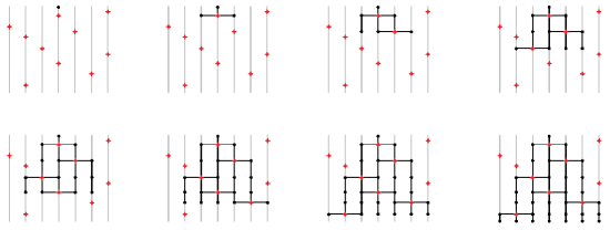
Figure 1. Iterative construction of the cone of dependence with $\mathcal{G}=\mathbb{Z}$ and $\mathcal{N}_{j}=j+\left\{-1,0,1\right\}$. The arrow of time points up. The red markers indicate the $\mathbf{Update}$ set and the black ones represent the consecutive sets $K_{n}$. The $\mathbf{Cone}$ consists of vertical black lines in the last panel.

The interpretation of these objects is as follows. Whenever a clock rings at site $j$ its state is updated according to some rule that takes into account the states of sites in $\mathcal{N}_{j}$. Thus to determine the state at points $\left\{t\right\}\times K$ we must traverse the space-time backward in time, marking the relevant update times and expanding the set of points that have a causal link with $(t,j)$. Here $(t_{n})_{n<\infty}$ are these update times and $(J_{n})_{n<\infty}$ are the sets of sites in the cone that are updated. We naturally extend this construction to finite $K\subseteq\mathcal{G}$ by setting

$$\mathbf{Cone}\left(t,K\right):=\bigcup_{j\in K}\mathbf{Cone}\left(t,j\right).$$

Definition 2.2 (Causality).

A graph-clock pair $\left(\mathcal{G},\mathcal{C}\right)$ is causal if and only if for all $(t,j)\in\mathbb{R}_{+}\times\mathcal{G}$

$$\mathbb{P}\left(\mathbf{Cone}(t,j)\cap\left\{0\right\}\times\mathcal{G}\neq\varnothing\right)=1.$$

Put simply a graph-clock pair is causal if and only if the recurrence from the construction of the cone almost surely halts ($t_{n}$ hits $0$) after finitely many steps. These are the graph-clock pairs for which it is possible to construct an interacting particle system. The idea behind this definition is not new - we only formalize it and give it a name.

Example 2.3.

For any finite graph $\mathcal{G}$ and any clock $\mathcal{C}$ the graph-clock pair $\left(\mathcal{G,\mathcal{C}}\right)$ is causal.

Example 2.4.

For any graph $\mathcal{G}$ the graph-clock pair $\left(\mathcal{G},\delta_{1}\right)$ is causal.

Example 2.5.

If there exists finite $\mathcal{N}\subset\mathbb{Z}^{d}$ such that $\mathcal{N}_{j}\subseteq j+\mathcal{N}$ for all $j$ then the graph-clock pair $\left(\mathbb{Z}^{d},\text{Exp}(1)\right)$ is causal.

Example 2.6.

If the clock is such that $\mathcal{C}(\left[0,t\right])>0$ for all $t>0$ and there exists $j\in\mathcal{G}$ such that $\left|\mathcal{N}_{j}\right|=\infty$ then $\left(\mathcal{G},\mathcal{C}\right)$ is not causal. As a consequence, the exponential clock requires a graph with finite neighborhoods.

Example 2.7.

It is possible for $\left(\mathcal{G},\text{Exp}(1)\right)$ to be causal even if $\sup_{j}\left|\mathcal{N}_{j}\right|=\infty$. Take $\mathcal{G}=\mathbb{Z}$ and $\mathcal{N}_{j}=\left\{0,\dots,j\right\}$. Here every cone of dependence is spatially bounded i.e. for any $t\geq 0$ we have

$$\mathbf{Cone}(t,j)\subseteq[0,t]\times\left\{0,\dots,j\right\}.$$

This, of course, implies causality since locally the graph is indistinguishable from a finite one.

Definition 2.8 (Transition matrix).

• Let $\mathcal{A}$ be a countable set, which we will call an alphabet.

• For every $j\in\mathcal{G}$ and $\sigma\in\mathcal{A}^{\mathcal{N}_{j}}$ let $P_{j}\left(\cdot\,|\,\sigma\right)$ be a probability distribution on $\mathcal{A}$. We will call $P=\left(\left(P_{j}\left(\cdot\,|\,\sigma\right)\right)_{\sigma\in\mathcal{A}^{\mathcal{N}(j)}}\right)_{j\in\mathcal{G}}$ a transition matrix.

Now for a given distribution $\mu_{0}$ on $\mathcal{A}^{\mathcal{G}}$, we will define its trajectory under an interacting particle system. We will do it by explicitly constructing a process $\left(\zeta_{t}\right)_{t\geq 0}$ on $\mathcal{A}^{\mathcal{G}}$ that agrees with $\mu_{0}$ at time $0$.

Definition 2.9 (Trajectory of IPS).

The construction of $\zeta_{t}$ is recursive and follows three conditions.

• The initial configuration $\zeta_{0}$ is distributed according to the initial distribution $\mu_{0}$.

• The state at site $j$ can only be updated when its respective clock rings i.e.
  if $t\in\left[\tau_{n}^{j},\tau_{n+1}^{j}\right)$ then $\zeta_{t}(j)=\zeta_{\tau_{n}^{j}}(j)$.

• The random variable $\zeta_{\tau_{n}^{j}}(j)$ is sampled from the $P_{j}(\,\cdot\;|\;\zeta_{\tau_{n}^{j-}})$ distribution independently of everything else. We use the convention that for a given stopping time $\tau$ the $\zeta_{\tau^{-}}$ denotes the left-side limit of $\left(\zeta_{t}\right)_{t<\tau}$ random variables.

Since $\left(\mathcal{G},C\right)$ is causal the recursion above will define $\zeta_{\tau_{n}^{j}}(j)$ for any $(j,n)$ in finitely many steps. Additionally, since the range of $C$ lies in $(0,\infty)$ then for every $t\geq 0$ and $j\in\mathcal{G}$ there exists $n$ such that $t\in\left[\tau_{n}^{j},\tau_{n+1}^{j}\right)$. Thus $\zeta_{t}$ is well defined.

Definition 2.10 (Interacting particle system).

An interacting particle system with a causal graph-clock pair $\left(\mathcal{G},\mathcal{C}\right)$ and transition matrix $P$ is the set of distributions of $\left(\zeta_{t}\right)_{t\geq 0}$ indexed by all initial distributions. We denote it by $\text{IPS}\left(P,\mathcal{C}\right)$.

For convenience, we will slightly abuse the notation.

Notation.

• If the distribution of a trajectory $\left(\zeta_{t}\right)_{t\geq 0}$ is a member of $\text{IPS}\left(P,\mathcal{C}\right)$ then we also write

  $$\left(\zeta_{t}\right)_{t\geq 0}\in\text{IPS}\left(P,\mathcal{C}\right).$$

• We will denote $\mu P_{t}$ as the distribution of $\zeta_{t}$ given $\zeta_{0}$ is distributed according to $\mu$.

• $\text{IPS}\left(P\right):=\text{IPS}\left(P,\text{Exp}(1)\right)$

• $\text{PCA}\left(P\right):=\text{IPS}\left(P,\delta_{1}\right)$.

The PCA stands for probabilistic cellular automata - the discrete-time version of interacting particle systems.

The last notions that need to be introduced are invariant measures, ergodicity, and covariance decay.

Definition 2.11 (Invariant measure).

An invariant measure of an $\text{IPS}\left(P,\mathcal{C}\right)$ is any distribution $\mu$ on $\mathcal{A}^{\mathcal{G}}$ such that $\mu P_{t}=\mu$ for all $t\geq 0$.

It is the general case that an IPS will have at least one invariant measure. It is always the case when the clock is memoryless (so it’s either geometric or exponential) and the neighborhoods of interaction $\mathcal{N}_{j}$ are finite for all $j\in\mathcal{G}$. In this case, the $\left(P_{t}\right)_{t\geq 0}$ (or $t\in\mathbb{N}$ when time is discrete) operators form a Markov semigroup on continuous functions on $\mathcal{A}^{\mathcal{G}}$ equipped with the product topology of discrete $\mathcal{A}$. For geometric clocks, the existence of an invariant measure follows immediately from Shauder’s fixed-point theorem applied to the $P_{1}$ operator. The proof for exponential clocks may be found in [Lig05](Proposition $1.8$ on page 10).

Definition 2.12 (Attractive invariant measure).

An invariant measure $\mu$ of an $\text{IPS}\left(P,\mathcal{C}\right)$ is attractive if for any other distribution $\nu$ we have convergence in distribution

$$\nu P_{t}\Rightarrow\mu.$$

Definition 2.13 (Ergodicity).

An $\text{IPS}(P,\mathcal{C})$ is said to be ergodic if it has an attractive measure $\mu$. It is exponentially ergodic with rate $\alpha$ if for every finite $S\subseteq\mathcal{G}$ there exists a constant $C_{S}\geq 0$ such that for any $A\subset\mathcal{A}^{\mathcal{G}}$ - cylinder set with support $S$ it holds that

$$\sup_{\nu}\left|\nu P_{t}\left(A\right)-\mu(A)\right|\leq C_{S}\cdot e^{-\alpha t}.$$

Definition 2.14 (Covariance decay).

An $\text{IPS}(P,\mathcal{C})$ is said to have (temporal) covariance decay if and only if for all $f,g\in F$ and initial distributions

$$\mathrm{Cov}\left(f\left(\zeta_{0}\right),\,g\left(\zeta_{t}\right)\right)\xrightarrow{t\rightarrow\infty}0.$$

This decay is said to be uniform if and only if additionally for all $f,g\in F$

$$\sup_{\left(\zeta_{t}\right)_{t\geq 0}\in\text{IPS}(P,\mathcal{C})}\left|\mathrm{Cov}\left(f\left(\zeta_{0}\right),\,g\left(\zeta_{t}\right)\right)\right|\xrightarrow{t\rightarrow\infty}0.$$

and exponential when there exist $\alpha>0$ and constants $C(f,g)$ such that for all initial distributions

$$\left|\mathrm{Cov}\left(f\left(\zeta_{0}\right),\,g\left(\zeta_{t}\right)\right)\right|\leq C(f,g)\cdot e^{-\alpha t}.$$

Remark 2.15.

(Exponential) covariance decay and (exponential) ergodicity are equivalent.

3. Time Scaling

The main goal of this article is the study of the ergodicity of IPS. It natural question to ask under which transformations of the transition matrix ergodicity is preserved. There is an obvious invariant: Re-scaling time cannot change ergodicity. In this section we explain what re-scaling in time means for the associated transition matrix. The main result of this section, namely the time-scaling lemma, shows that it is equivalent to taking a convex combination of the original transition matrix with the identity matrix. As we will see in later sections this simple observation has surprising consequences.

Lemma 3.1 (Time-scaling).

Let us consider a given transition matrix $P$ (cf. Defintion 2.10) and let $I$ denote the identity transition matrix. Then for all $\lambda\in(0,1]$ it holds:

$$\left(\zeta_{t}\right)_{t\geq 0}\in\text{IPS}\left(P\right)\text{ if and only if }\left(\zeta_{\frac{t}{\lambda}}\right)_{t\geq 0}\in\text{IPS}\left(\lambda P+(1-\lambda))I\right).$$

The use of this lemma is that the set of invariant measures and properties like ergodicity are preserved under rescaling time. This allows us to extend past results about these properties which we do in the next section.

Corollary 3.2.

Ergodicity and the set of invariant measures are the same for $\text{IPS}(P)$ and
$\text{IPS}(\lambda P+\left(1-\lambda\right)I)$. If they are ergodic then the ratio of their rates of covariance decay is $\lambda$.

Proof of Time-scaling Lemma.

Since the statement of the lemma concerns only the distribution of $\left(\zeta_{t}\right)_{t\geq 0}$ we may construct this random variable arbitrarily. To do this we will first construct trajectory $\xi_{t}$ of $\text{IPS}\left(\lambda P+(1-\lambda))I\right)$. Let $\left(\rho_{n}^{j}\right)_{n<\infty}^{j\in\mathcal{G}}$ be i.i.d. and distributed according to $\text{Exp}(1)$ and set $\tau_{n}^{j}:=\rho_{1}^{j}+\dots\rho_{n}^{j}$. Define additional i.i.d. $\text{Bern}(\lambda)$ variables $\left(V_{n}^{j}\right)_{n<\infty}^{j\in\mathcal{G}}$ and independent from them i.i.d. $\text{Unif}[0,1]$ variables $\left(U_{n}^{j}\right)_{n<\infty}^{j\in\mathcal{G}}$. Now set:

• The initial configuration $\xi_{0}:=\zeta_{0}$.

• If $t\in\left[\tau_{n}^{j},\tau_{n+1}^{j}\right)$ then $\xi_{t}(j):=\xi_{\tau_{n}^{j}}(j)$.

• The recursion principle

  $$\xi_{\tau_{n+1}^{j}}(j):=V_{n+1}^{j}\cdot F_{j}\left(\xi_{\tau_{n+1}^{j-}}\left(\mathcal{N}_{j}\right),U_{n+1}^{j}\right)+\left(1-V_{n+1}^{j}\right)\cdot\xi_{\tau_{n}^{j}}(j),$$

  where $F_{j}:\mathcal{A}^{\mathcal{G}}\times\left[0,1\right]\rightarrow\mathcal{A}$ are such that

  $$\mathbb{P}\left(F_{j}\left(\sigma,U_{n}^{j}\right)=a\right)=P_{j}\left(a\;|\;\sigma\right)$$

  for any $j\in\mathcal{G}$, $a\in\mathcal{A}$ and $\sigma\in\mathcal{A}^{\mathcal{G}}$.

The random variables $V_{n}^{j}$ act as blockers - when a clock rings at site $j$ it will fail to update (or rather, be updated by $I$) with probability $1-\lambda$.
By construction $\left(\xi_{t}\right)_{t\geq 0}\in\text{IPS}\left(\lambda P+(1-\lambda)I\right)$. Now define stopping times $\left(\pi_{n}^{j}\right)_{n<\infty}^{j\in\mathcal{G}}$ by $\pi_{0}^{j}:=0$ and

$$\pi_{n+1}^{j}:=\min\left\{\tau_{k}^{j}>\pi_{n}^{j}\,:\,V_{k}^{j}=1\right\}.$$

Put simply $\left(\pi_{n}^{j}\right)_{n<\infty}$ skips the failed updates. The trajectory $\left(\xi_{t}\right)_{t\geq 0}$ satisfies

• The initial configuration is still $\xi_{0}=\zeta_{0}$.

• If $t\in\left[\pi_{n}^{j},\pi_{n+1}^{j}\right)$ then $\xi_{t}(j)=\xi_{\pi_{n}^{j}}(j)$.

• The recursion principle

  $$\xi_{\pi_{n+1}^{j}}(j)=F_{j}\left(\xi_{\pi_{n+1}^{j-}}\left(\mathcal{N}_{j}\right),U_{n+1}^{j}\right).$$

Therefore if $\left(\pi_{n}^{j}\right)_{n<\infty}$ has independent, stationary increments then $\left(\xi_{t}\right)_{t\geq 0}$ is a trajectory of an IPS with transition matrix $P$ and the distribution of those increments as a clock. We will show that these increments are independent and that their distribution is exponential. Let $\mathcal{F}_{t}$ be the canonical $\sigma$-algebra of events up to time $t$.

$$\mathbb{P}\left(\pi_{n+1}^{j}-\pi_{n}^{j}>t\,|\,\mathcal{F}_{\pi_{n}^{j}}\right)=\sum_{k=0}^{\infty}\mathbbm{1}\left({\pi_{n}^{j}=\tau_{k}^{j}}\right)\mathbb{E}\left[\mathbbm{1}\left(\pi_{n+1}^{j}-\pi_{n}^{j}>t\right)\;|\;\mathcal{F}_{\pi_{n}^{j}}\right]=$$

$$\sum_{k=0}^{\infty}\mathbbm{1}\left({\pi_{n}^{j}=\tau_{k}^{j}}\right)\mathbb{E}\left[\sum_{m=1}^{\infty}\mathbbm{1}\left(V_{k+1}^{j},\dots,V_{k+m-1}^{j}=0,V_{k+m}^{j}=1\right)\cdot\mathbbm{1}\left(\rho_{k+1}^{j}+\dots+\rho_{k+m}^{j}>t\right)\;|\;\mathcal{F}_{\pi_{n}^{j}}\right]$$

Variables in the expectation are independent from the $\sigma$-algebra on the event $\left\{\pi_{n}^{j}=\tau_{k}^{j}\right\}$. Additionally, since $V^{\prime}s$ are i.i.d. $\text{Bern}(\lambda)$ and $\rho^{\prime}s$ are i.i.d. $\text{Exp}(1)$ variables then the above equals

$$\sum_{k=0}^{\infty}\mathbbm{1}\left({\pi_{n}^{j}=\tau_{k}^{j}}\right)\sum_{m=1}^{\infty}\lambda(1-\lambda)^{m-1}\mathbb{P}\left(\text{Gamma}(m,1)>t\right)=$$

$$\sum_{m=1}^{\infty}\lambda(1-\lambda)^{m-1}\mathbb{P}\left(\text{Gamma}(m,1)>t\right)=\sum_{m=1}^{\infty}\lambda(1-\lambda)^{m-1}\int_{[t,\infty)}\frac{1}{(m-1)!}x^{m-1}e^{-x}dx=$$

$$\int_{[t,\infty)}\lambda e^{-x}\sum_{m=0}^{\infty}\frac{\left(x(1-\lambda)\right)^{m}}{m!}dx=\int_{[t,\infty)}\lambda e^{-\lambda x}dx=\mathbb{P}\left(\text{Exp}(\lambda)>t\right).$$

Since the result is a constant with respect to $\mathcal{F}_{\pi_{n}^{j}}$ then the increment $\pi_{n+1}^{j}-\pi_{n}^{j}$ is independent from that $\sigma$-algebra. In addition we have shown that its distribution is $\text{Exp}(\lambda)$. As argued before this implies that

$$\left(\xi_{t}\right)_{t\geq 0}\in\text{IPS}\left(P,\text{Exp}(\lambda)\right).$$

Setting $\zeta_{t}=\xi_{\lambda t}$ yields the desired result. ∎

The following example shows that a similar result does not hold for PCAs.

Example 3.3.

Consider $\mathcal{G}=\mathbb{Z}^{d},\mathcal{A}=\left\{-1,+1\right\}$ and a transition matrices $P,Q$

$$P_{j}(+1\;|\;\sigma)=\mathbbm{1}\left(\sigma(j)=-1\right)$$

$$Q_{j}(+1\;|\;\sigma)=\frac{1}{2}.$$

The rule $P$ flips state while $Q$ chooses it independently from everything. By the Time-scaling Lemma, $\text{IPS}(P)$ is just $\text{IPS}(Q)$ with time sped up by a factor of $\frac{1}{\lambda}=2$. The same is not true for $\text{PCA}(P)$ and $\text{PCA}(Q)$. Notice that $\text{PCA}(P)$ has a periodic trajectory "all +1" followed by "all -1", while $\text{PCA}(Q)$ turns every initial distribution into the $\text{Bern}\left(\frac{1}{2}\right)$ product measure after a single time-step.

4. Extensions of previous results

The Time-scaling Lemma implies that properties of an IPS that are invariant under rescaling time are the same for all IPS whose transition matrices lie on a line crossing the identity matrix. These properties include the invariance of a given measure, its limit under $P_{t}$, and (exponential) ergodicity. Thus to prove that an $\text{IPS}(P)$ has any of these properties it suffices to find some other $\text{IPS}(Q)$ with the transition matrix of the form $Q=\lambda P+\left(1-\lambda\right)I$ where $\lambda>0$ which has it. It allows us to extend many previous results with little additional effort. The strategy for this is straightforward - if a theorem states that IPS in some subset of the parameter space are ergodic then we can extend this subset along lines with roots at identity and have ergodicity proven in this (hopefully) larger subset. In this section, we will go through a few theorems about IPS and strengthen them.

We start with extending a couple of results on monotone IPS. This is a well-studied type of IPS with examples including the voter model, contact process, and ferromagnetic stochastic Ising models. As a consequence much is known about their behavior and there are many general results that can be extended with the time-scaling trick. To set the stage we will require a few definitions.

Notation.

For a transition matrix $P$ with a linearly ordered alphabet $\left(\mathcal{A},\geq\right)$ we will write

$$P\left(a_{+}\;|\;\zeta\right):=\sum_{b\geq a}P\left(b\;|\;\zeta\right).$$

Definition 4.1 (Domination).

For two transition matrices $P,Q$ over the same graph $\mathcal{G}$ and a linearly ordered alphabet $\left(\mathcal{A},\geq\right)$ we will say that $P$ dominates $Q$ if for all $a\in\mathcal{A}$ it holds that

$$P_{j}\left(a_{+}\,|\,\zeta\right)\geq Q_{j}\left(a_{+}\,|\,\xi\right)\text{ whenever }\zeta\geq\xi.$$

We will also say that an $\text{IPS}(P)$ dominates $\text{IPS}(Q)$ if $P$ dominates $Q$.

Definition 4.2 (Monotonicity).

A transition matrix is monotone if it dominates itself. We will also say that an IPS is monotone if its transition matrix is.

We will now discuss a few fundamental results regarding monotone IPS that provide great aid in their analysis. Informally, the first lemma states that if one IPS dominates another then their evolutions preserve stochastic dominance between their trajectories.

Lemma 4.3 (Domination lemma).

Let $\text{IPS}(P)$ dominate $\text{IPS}(Q)$. Then for any pair of initial distributions that satisfy $\zeta_{0}\geq\xi_{0}$ their trajectories $\left(\zeta_{t}\right)_{t\geq 0}$ and $\left(\xi_{t}\right)_{t\geq 0}$ under $\text{IPS}(P)$ and $\text{IPS}(Q)$ respectively can be constructed in such a way that $\zeta_{t}\geq\xi_{t}$ for all $t\geq 0$.

Proof of Domination Lemma.

We show that the construction given in Section 2 satisfies this condition. First, we let $\zeta$ and $\xi$ share the clock and update random variables ($\tau$s and $U$s). Then wet set the update functions $\left(f_{j}\right)_{j\in\mathcal{G}},\left(g_{j}\right)_{j\in\mathcal{G}}$ to be the non-decreasing step functions on $[0,1]$ satisfying for all $\sigma\in\mathcal{A}^{\mathcal{G}}$ and $a\in\mathcal{A}$

$$\mathbb{P}\left(f_{j}\left(\sigma,U_{n}^{j}\right)=a\right)=P_{j}\left(a\,|\,\sigma\right)\;\,$$

$$\mathbb{P}\left(g_{j}\left(\sigma,U_{n}^{j}\right)=a\right)=Q_{j}\left(a\,|\,\sigma\right).$$

Then the $\zeta\geq\xi$ condition is preserved by each update. ∎

Armed with this lemma we now prove the first theorem about monotone IPS. It states that the distributions of trajectories of monotone IPS are themselves monotone.

Notation.

• When the graph is known from the context then for any $a\in\mathcal{A}$ we will shorten the Dirac deltas

  $$\delta_{a}:=\delta_{\left\{a\right\}^{\mathcal{G}}}.$$

• For a linearly-ordered alphabet, we will denote its minimal and maximal elements (if they exist) as $\underaccent{\bar}{a}$ and $\bar{a}$ respectively.

Theorem 4.4.

If the $\text{IPS}(P)$ is monotone then the following holds:

1. For any increasing event $A$ (i.e. one such that if $\zeta\geq\xi$ and $\xi\in A$ then $\zeta\in A$) the function

   $$t\mapsto\delta_{a}P_{t}\left(A\right)$$

   is non-increasing for $a=\bar{a}$ and non-decreasing for $a=\underaccent{\bar}{a}$ (provided these exist).

2. The weak limits of $\left(\delta_{a}P_{t}\right)_{t\geq 0}$ for $a\in\left\{\underaccent{\bar}{a},\bar{a}\right\}$ exist. These limits will be denoted as $\mu_{\underaccent{\bar}{a}}$ and $\mu_{\bar{a}}$ respectively.

3. These limits coincide if and only if $\text{IPS}(P)$ is ergodic.

Note that this result implies that for monotone IPS uniqueness of the invariant measure is equivalent to ergodicity. In general, whether this happens is an open problem.

Proof of Theorem 4.4.

Argument for (1): Without loss of generality let $a=\bar{a}$. Pick any $t\geq s\geq 0$. Let $\zeta_{0}=a$ and $\xi_{0}$ be distributed according to $\delta_{a}P_{t-s}$. We have $\zeta_{0}\geq\xi_{0}$ so by monotonicity of $P$ and the Lemma 4.3 we can construct their respective trajectories under $P$ in such a way that $\zeta_{u}\geq\xi_{u}$ for all $u\geq 0$. In particular $\zeta_{s}\geq\xi_{s}$. This in turn implies

$$\delta_{a}P_{s}\left(A\right)=\mathbb{P}\left(\zeta_{s}\in A\right)\geq\mathbb{P}\left(\xi_{s}\in A\right)=\delta_{a}P_{t}\left(A\right).$$

Argument for (2): It is an easy exercise to check that any measure $\mu$ on $\mathcal{A}^{G}$ is uniquely determined by its values of

$$\mu\left(\sigma\geq C\text{ on }K\right)$$

for all possible cylinders $C$ and their supports $K$. The measure of any cylinder with finite support is a finite linear combination of terms of this form. The sequence

$$\left(\delta_{a}P_{t}\left(\sigma\geq C\text{ on }K\right)\right)_{t\geq 0}$$

is monotone by $(1)$ because these are increasing events. It is also bounded so it has a limit. Thus the limit of $\delta_{a}P_{t}(C)$ exists for any $C$, which is exactly convergence in distribution.

Argument for (3): The Lemma 4.3 again implies that for any measure $\mu$

$$\delta_{\bar{a}}P_{t}\left(\sigma\geq C\text{ on }K\right)\geq\mu P_{t}\left(\sigma\geq C\text{ on }K\right)\geq\delta_{\underaccent{\bar}{a}}P_{t}\left(\sigma\geq C\text{ on }K\right)$$

for all $t\geq 0$. As a consequence

$$\mu_{\bar{a}}\left(\sigma\geq C\text{ on }K\right)\geq\lim_{t\rightarrow\infty}\mu P_{t}\left(\sigma\geq C\text{ on }K\right)\geq\mu_{\underaccent{\bar}{a}}\left(\sigma\geq C\text{ on }K\right).$$

If $\mu_{\underaccent{\bar}{a}}=\mu_{\bar{a}}$ then the limits of $\mu P_{t}\left(C\right)$ exist and agree with them. This implies that the limiting measure of $\mu P_{t}$ is $\mu_{a}=\mu_{b}$. ∎

Let us discuss one more extension of a criterion for the ergodicity of monotone IPS. More precisely, we will extend a result by Gray (see Theorem 4.6 below) using the time-scaling trick. The improved version (Theorem 4.10 below) will be used later in Section 6. To state the theorem we need one additional definition.

Definition 4.5 (Positive rates).

A transition matrix $P$ has positive rates if it differs from the identity on every entry.

The name comes from the original construction of interacting particle systems with alphabet $\left\{0,1\right\}$, where instead of a transition matrix determining updates each site had a clock with an exponential rate that varied depending on the site’s neighborhood. Whenever this clock rang the site flipped its state between $\left\{0,1\right\}$. Positive rates, in this case, mean that flipping the state is possible in any neighborhood. This translates exactly to our definition.

Theorem 4.6 (Larry Gray).

[Gra82] (Theorem $1$, page 397)
Every one-dimensional, periodic, monotone IPS with nearest-neighbor interactions, positive rates and alphabet of size two is ergodic.

A reader familiar with Gray’s paper may notice that this statement is seemingly stronger than the one cited. The difference comes down to the construction of IPS. This is explained in detail in Section 7.1 in the appendix.

Now, we apply the Time-scaling Lemma to extend the results of Theorem 4.4 and Gray’s Theorem to IPS which are not monotone. Notice that all the properties proven in these theorems are invariant under rescaling time. Thus by the Time-scaling Lemma an $\text{IPS}(P)$ will have them if there exists $\lambda>0$ such that $\text{IPS}\left(\lambda P+\left(1-\lambda\right)I\right)$ is monotone. This leads to a condition that is weaker than monotonicity and we name it accordingly - weak monotonicity.

Definition 4.7 (Weak domination).

For two transition matrices $P,Q$ over the same graph $\mathcal{G}$ and a linearly ordered alphabet $\left(\mathcal{A},\geq\right)$ we will say that $P$ weakly dominates $Q$ if for all $a\in\mathcal{A}$ it holds that

$$P_{j}\left(a_{+}\,|\,\zeta\right)\geq Q_{j}\left(a_{+}\,|\,\xi\right)\text{ whenever }\left\{\begin{array}[]{l}\zeta\geq\xi\\ \zeta(j),\xi(j)\geq a\text{ or }\zeta(j),\xi(j)<a\end{array}\right..$$

This is a strictly weaker condition than domination - if $\zeta(j)>\xi(j)$ then for every $a\in\mathcal{A}$ such that $\zeta(j)\geq a>\xi(j)$ the inequality $P_{j}\left(a_{+}\,|\,\zeta\right)\geq Q_{j}\left(a_{+}\,|\,\xi\right)$ is no longer required.

Definition 4.8 (Weak monotonicity).

A transition matrix is weakly monotone if it dominates itself weakly.

Weak monotonicity is of course a weaker condition than monotonicity. For example in the case of nearest neighbor IPS on $\mathbb{Z}$ with an alphabet of size two weak monotonicity requires $8$ independent inequalities to be satisfied, while monotonicity requires $12$. However, we can use the Time-scaling Lemma to prove that they are equivalent when studying ergodic properties. First, let us verify that weak monotonicity is the correct extension of monotonicity.

Lemma 4.9.

If $\text{IPS}(P)$ is weakly monotone then for $\lambda\leq\frac{1}{2}$ the $\text{IPS}\left(\lambda P+\left(1-\lambda\right)I\right)$ is monotone.

Proof of Lemma 4.9.

For any $a\in\mathcal{A}$

$$\left(\lambda P+\left(1-\lambda\right)I\right)_{j}\left(a_{+}\;|\;\zeta\right)=\lambda P_{j}\left(a_{+}\;|\;\xi\right)+\left(1-\lambda\right)\mathbbm{1}\left(\zeta(j)\geq a\right).$$

For any $\zeta\geq\xi$ there are two cases to consider:

• If $\zeta(j)\geq a>\xi(j)$ then for $\lambda\leq\frac{1}{2}$ the condition

  $${\lambda P_{j}\left(a_{+}\;|\;\zeta\right)+\left(1-\lambda\right)I_{j}}\left(a_{+}\;|\;\zeta\right)\geq\lambda P_{j}\left(a_{+}\;|\;\xi\right)+\left(1-\lambda\right)I_{j}\left(a_{+}\;|\;\xi\right)$$

  is satisfied regardless of $P_{j}$.

• If on the other hand $\zeta(j)$ and $\xi(j)$ are both greater or both less than $a$ then the condition

  $$\left(\lambda P+\left(1-\lambda\right)I\right)_{j}\left(a_{+}\;|\;\zeta\right)\geq\left(\lambda P+\left(1-\lambda\right)I\right)_{j}\left(a_{+}\;|\;\xi\right)$$

  is equivalent to

  $$P_{j}\left(a_{+}\;|\;\zeta\right)\geq P_{j}\left(a_{+}\;|\;\xi\right).$$

Thus if $\text{IPS}(P)$ is weakly monotone then for $\lambda\leq\frac{1}{2}$ the $\text{IPS}(\lambda P+\left(1-\lambda\right)I)$ is monotone. ∎

Theorem 4.10 (Extension of results for monotone IPS).

Weak monotonicity is sufficient for the results of Theorem 4.4 and Gray’s Theorem to hold.

Proof of Theorem 4.10.

By the Time-scaling Lemma, it suffices to show that there exists a $\lambda>0$ such that $\lambda P+\left(1-\lambda\right)I$ is monotone. By Lemma 4.9 any $\lambda$ between $0$ and $\frac{1}{2}$ works. Notice that the positive rates property is preserved by convex combinations with identity. ∎

We depart from the realm of monotone IPS. The next two theorems we will be extending come from David Griffeath’s lecture notes on "Additive and Cancellative Interacting Particle Systems"[Gri78], where the exponential ergodicity of these types of IPS are proven, assuming the presence of noise.

There are many ways to construct a trajectory of an IPS and the construction in Griffeath’s work differs greatly from our own. As a result, it’s not immediately obvious what a transition matrix of an additive or cancellative IPS looks like. We answer this question below.

Theorem 4.11 (Griffeath).

[Gri78] (Corollary 2.5, page 20)
Let $\text{IPS}(P)$ be homogenous over $\mathbb{Z}^{d}$ with positive rates and alphabet $\left\{0,1\right\}$. If $P$ is a convex combination of matrices of the form

$$P_{S}\left(1\,|\,\sigma\right)=\left\{\begin{array}[]{lr}1&S\cap\sigma^{-1}\left(1\right)\neq\varnothing\\ 0&S\cap\sigma^{-1}\left(1\right)=\varnothing\end{array}\right.\textit{ for any }S\subseteq\mathcal{N}$$

and the $\mathbf{1}$ matrix then $\text{IPS}(P)$ is exponentially ergodic. The rate of ergodicity is at least as large as the coefficient of the $\mathbf{1}$ matrix in the above convex combination.

Theorem 4.12 (Griffeath).

[Gri78] (Corollary 2.3, page 72)
Let $\text{IPS}(P)$ be homogenous over $\mathbb{Z}^{d}$ with positive rates and alphabet $\left\{0,1\right\}$. If $P$ is a convex combination of matrices of the form

$$P_{0,S}\left(1\,|\,\sigma\right)=\left|S\cap\sigma^{-1}\left(1\right)\right|\left(\text{mod }2\right)$$

$$P_{1,S}\left(1\,|\,\sigma\right)=1-\left|S\cap\sigma^{-1}\left(1\right)\right|\left(\text{mod }2\right)$$

then $\text{IPS}(P)$ is exponentially ergodic. The rate of ergodicity is at least as large as twice the coefficient of the $\mathbf{1}$ matrix in the above convex combination.

The details of the translation from Griffeath’s construction of additive/cancellative IPS can be found in Sections 7.2 and  7.3 in the appendix. Note that all of the matrices $P_{S}$ are deterministic and in the additive case - monotone. The way we extend these theorems remains the same - we characterize the $\text{IPS}(P)$ for which there exists another of the form $\text{IPS}(\lambda P+\left(1-\lambda\right)I)$ which satisfies the conditions in either theorem.

Theorem 4.13 (Extension of Griffeath’s theorems).

Theorems 4.11 and 4.12 also hold when the coefficient of $P_{\left\{0\right\}}$ (i.e. the identity) is allowed to be negative (the coefficients must still sum to $1$).

Proof of Theorem 4.13.

Let $P$ be a transition matrix with positive rates, expressable as

$$P=\alpha\mathbf{1}+\sum_{S\subseteq\mathcal{N}}\lambda_{S}P_{S}$$

where $\alpha+\sum\lambda_{S}=1$ and $\lambda_{S}\geq 0$, with the possible exception of $\lambda_{\left\{0\right\}}$. Consider the transition matrix

$$Q=\lambda P+\left(1-\lambda\right)I=\lambda\cdot\alpha\mathbf{1}+\sum_{S\subseteq\mathcal{N}}\lambda\cdot\lambda_{S}P_{S}+\left(1-\lambda\right)P_{\left\{0\right\}}.$$

For $\lambda$ sufficiently close to $0$ the coefficient of $P_{\left\{0\right\}}=I$ becomes positive, which means that by Theorem 4.11 (or 4.12) the $\text{IPS}(Q)$ is exponentially ergodic with rate $\lambda\cdot\alpha$ (or $2\lambda\cdot\alpha$). We finish off with the Time-scaling Lemma which implies that $\text{IPS}(P)$ is exponentially ergodic with rate $\alpha$ (or $2\alpha$). ∎

5. Covariance Decay Criterion

In this section, we develop a method of proving exponential covariance decay of IPS. The resulting criterion is similar to a result by A.M. Leontovitch and L.N. Vaserstein [VNLM70] for PCAs. For a reference in English see Chapter $4$ and Chapter $7$ of [TVS⁺90]. Our contribution is translating the criterion to continuous time, generalizing the result, and giving an independent proof. Our result for IPS is more general as working in continuous time allows the application of the time-scaling trick. Additionally, our proof demands fewer assumptions on the underlying graph structure. However, our argument uses similar calculations as in the case of PCAs.

The main idea is as follows. Consider a covariance between two functions on the configuration space, one taken when the process is at time $0$ and one at time $t$ like so:

$$\mathrm{Cov}\left(f(\zeta_{0}),\,g(\zeta_{t})\right).$$

Increasing $t$ has the effect of adding more updates to the past of $\zeta_{t}$. If one could prove that each of those updates acts like a contraction on such covariances then an explicit rate of their decay could be deduced. The argument is recursive which presents technical challenges when applying to continuous time, where the times of updates are random and almost surely not well-ordered. Aside from that hiccup, the proof is a straightforward calculation.

Before we can state our theorem we need to define a few new objects. We will start with the space of "local" functions for a given alphabet and graph.

Notation.

• For $f:\mathcal{A}^{\mathcal{G}}\rightarrow\mathbb{R}$ define the domain of $f$ as the minimal set of coordinates on which the value of $f$ depends. Denote it as $\text{Dom}(f)$.

• For a graph $\mathcal{G}$ and alphabet $\mathcal{A}$ let

  $$F(\mathcal{A},\mathcal{G})=\left\{f:\mathcal{A}^{\mathcal{G}}\rightarrow\mathbb{R}\;:\;\left|\text{Dom}(f)\right|<\infty\right\}.$$

  Note that such functions are necessarily bounded and that they form a linear space. We will shorten it to $F$ when the alphabet and graph are known from the context.

Definition 5.1 (Representational semi-norm).

For any family $\mathcal{F}\subseteq F$ such that $\text{Span}\left(\mathcal{F}\right)=F$ we define a representational semi-norm on $F$ as follows:

$$\left\|f\right\|_{\mathcal{F}}:=\inf\left\{\sum_{1\leq k\leq n}\left|a_{k}\right|\;:\;\exists\left(g_{1},\dots,g_{n}\in\mathcal{F}\setminus\left\{\text{const.}\right\}\right)\left[\sum_{1\leq k\leq n}a_{k}\cdot g_{k}=f-\text{const.}\right]\right\}.$$

Definition 5.2 (Product basis).

Let $\mathcal{A}=\left\{-1,+1\right\}$. For any $A\in\mathbb{R}\setminus\left\{0\right\},B\in\mathbb{R}$ we will construct a family of functions

$$\mathcal{F}_{\Pi}(A,B)=\left\{\mbox{\scalebox{1.2}{$\chi$}}_{K}\;:\;K\subseteq\mathcal{G},\left|K\right|<\infty\right\},$$

where $\mbox{\scalebox{1.2}{$\chi$}}_{K}$ is defined as

$$\mbox{\scalebox{1.2}{$\chi$}}_{K}\left(\zeta\right):=\prod_{j\in K}A\left(B+\zeta(j)\right).$$

We will call $\mathcal{F}_{\Pi}$ a product basis of $F$ and the numbers $A$,$B$ its values. To convince yourself that $\text{Span}\left(\mathcal{F}_{\Pi}\right)=F$ notice that one can easily construct the indicator function of arbitrary cylinders by multiplying terms of the form

$$\frac{\mbox{\scalebox{1.2}{$\chi$}}_{\left\{j\right\}}}{2A}-\frac{B-1}{2},\textit{ and }-\frac{\mbox{\scalebox{1.2}{$\chi$}}_{\left\{j\right\}}}{2A}+\frac{B+1}{2}$$

and then expanding the result. Of course, these indicator functions span $F$ in the following way:

$$f(\zeta)=\sum_{\sigma\in\mathcal{A}^{\text{Dom}\left(f\right)}}f\left(\sigma\right)\mathbbm{1}\left(\zeta\left(\text{Dom}(f)\right)=\sigma\right).$$

Now we will prove that the representations in $\mathcal{F}_{\Pi}$ are unique making this family a basis. To see that it’s the case notice that one needs only prove that for any finite $K\subset\mathcal{G}$ the functions $\left(\mbox{\scalebox{1.2}{$\chi$}}_{L}\right)_{L\subseteq K}$ form a basis of $\mathbb{R}^{\left\{-1,1\right\}^{K}}$. Indeed if that was not the case then we would find a counterexample to their linear independence within some finite $K$. The dimension of $\mathbb{R}^{\left\{-1,1\right\}^{K}}$ is $2^{\left|K\right|}$ and there are exactly as many functions in $\left(\mbox{\scalebox{1.2}{$\chi$}}_{L}\right)_{L\subseteq K}$. Since they span $\mathbb{R}^{\left\{-1,1\right\}^{K}}$ they must be linearly independent.

Notation.

For convenience, we will write $\left\|\cdot\right\|_{\Pi}$ rather than $\left\|\cdot\right\|_{\mathcal{F}_{\Pi}}$.

Definition 5.3 (Update operators).

For an $\text{IPS}\left(P,\mathcal{C}\right)$ on $\mathcal{G}$ and any $j\in\mathcal{G}$ will define a linear operators $E_{j}:F\left(\mathcal{A},\mathcal{G}\right)\rightarrow F\left(\mathcal{A},\mathcal{G}\right)$ by

$$E_{j}(f)(\sigma):=\mathbb{E}\left[f\left(\zeta_{t}\right)\;|\;\zeta_{t^{-}}=\sigma\textit{ and }\left(t,j\right)\in\mathbf{Update}\right].$$

These are the one-step update operators, assuming that an update happened at site $j$. If $\mathcal{C}=\delta_{1}$ i.e. our IPS is a PCA then this operator is the same for all $j$. If the clock is $\text{Exp}(1)$ then at most one site is updated at a time almost surely and each site is equally likely to be the next one updated. This motivates the construction of

$$E(f):=\frac{1}{\left|\text{Dom}(f)\right|}\sum_{j\in\text{Dom}(f)}E_{j}(f).$$

This is the operator of expectation after one update occurs somewhere in the domain of a function.

Definition 5.4 (Update coefficients).

For any product basis let $\left(C_{j,S}\right)_{j\in\mathcal{G},S\subseteq\mathcal{N}_{j}}$ be the representational coefficients of $E_{j}\left(\mbox{\scalebox{1.2}{$\chi$}}_{\left\{j\right\}}\right)$ in this basis i.e.

$$E_{j}\left(\mbox{\scalebox{1.2}{$\chi$}}_{\left\{j\right\}}\right)=\sum_{S\subseteq\mathcal{N}_{j}}C_{j,S}\cdot\mbox{\scalebox{1.2}{$\chi$}}_{S}.$$

Theorem 5.5 (Leontovitch, Vaserstein).

[VNLM70](in Russian)
Let $R:=\max_{j\in\mathcal{G}}\left|\mathcal{N}_{j}\right|$ be finite and for a product basis with values $A,B$ denote

$$\gamma:=\max_{1\leq m\leq R}\left(1,\max\left(\left|A\right|,\left|B\right|\right)^{\frac{R}{m}-1},\left(\left|\frac{A^{m}-B^{m}}{A-B}\right|+\left|\frac{A^{m}B-AB^{m}}{A-B}\right|\right)^{\frac{R}{m}}\right).$$

If for a $PCA$ over graph $\mathcal{G}$ it holds that

$$\sup_{j\in\mathcal{G}}\sum_{S\subseteq\mathcal{N}_{j}}\left|C_{j,S}\right|<\frac{1}{\gamma},$$

then this $PCA$ is uniformly, exponentially ergodic.

We are now ready to state the main result of this section.

Theorem 5.6.

If there exists a product basis with values bounded by $\pm 1$ of different signs, for which the $\left(C_{j,\left\{j\right\}}\right)_{j\in\mathcal{G}}$ constants are uniformally bounded and

$$\alpha:=\sup_{j\in\mathcal{G}}\left(C_{j,\left\{j\right\}}+\sum_{\begin{array}[]{l}S\subseteq\mathcal{N}_{j}\\ S\neq\left\{j\right\}\end{array}}\left|C_{j,S}\right|\right)<1$$

then $\text{IPS}(P)$ has uniform, exponential covariance decay. Moreover for any $f,g\in F$ and $\zeta\in\text{IPS}(P)$

$$\left|\mathrm{Cov}\left(f(\zeta_{0}),\,g(\zeta_{t})\right)\right|\leq 2\left\|f\right\|_{\infty}\left\|g\right\|_{\Pi}e^{-\left(1-\alpha\right)t}.$$

This new proof does not require that $\left|\mathcal{N}_{j}\right|$s be uniformly bounded and relaxes the central inequality. The restriction of bases to the bounded non-monosigned ones is not necessary but it does make our result much cleaner with little loss of efficiency - in applications these bases happen to be the ones that give the most robust criteria for ergodicity anyway.

Proof of the Theorem 5.6.

The strategy for the proof is as follows. First, we will prove the result given the stronger inequality

$$\alpha:=\sup_{j\in\mathcal{G}}\sum_{S\subseteq\mathcal{N}_{j}}\left|C_{j,S}\right|<1.$$

Then the result with the weaker inequality will follow by the Time-scaling Lemma. To deal with updates one by one we will introduce auxiliary stopping times of updates happening in a given subset of $\mathcal{G}$. We will then show that every update in $K$ contracts the covariance of $\mathrm{Cov}\left(f(\zeta_{0}),\,\mbox{\scalebox{1.2}{$\chi$}}_{K}(\zeta_{t})\right)$. Once we have that we will estimate the distribution of the number of updates to a function up to a specified time and obtain an explicit bound for covariance decay. But first, we will introduce the following lemma that will allow us to contract covariances with updates later.

Lemma 5.7.

If the product basis $\mathcal{F}_{\Pi}$ has values bounded by $\pm 1$ of different signs then for all finite $K\subset\mathcal{G}$ it holds

$$\left\|E(\mbox{\scalebox{1.2}{$\chi$}}_{K})\right\|_{\Pi}\leq\sup_{j\in\mathcal{G}}\sum_{S\subseteq\mathcal{N}_{j}}\left|C_{j,S}\right|.$$

Proof of Lemma 5.7.

The proof is a straightforward calculation.

$$\left\|E(\mbox{\scalebox{1.2}{$\chi$}}_{K})\right\|_{\Pi}=\left\|\frac{1}{\left|K\right|}\sum_{j\in K}E_{j}(\mbox{\scalebox{1.2}{$\chi$}}_{K})\right\|_{\Pi}\leq\sup_{j\in K}\left\|E_{j}(\mbox{\scalebox{1.2}{$\chi$}}_{K})\right\|_{\Pi}.$$

This last term can be bounded as follows:

$$\left\|E_{j}\left(\mbox{\scalebox{1.2}{$\chi$}}_{K}\right)\right\|_{\Pi}=\left\|\sum_{S\subseteq\mathcal{N}_{j}}C_{j,s}\cdot\mbox{\scalebox{1.2}{$\chi$}}_{K\setminus\left\{j\right\}\triangle\left(j+S\right)}\cdot\mbox{\scalebox{1.2}{$\chi$}}_{K\setminus\left\{j\right\}\cap\left(j+S\right)}^{2}\right\|_{\Pi}\leq\sum_{S\subseteq\mathcal{N}_{j}}\left|C_{j,S}\right|.$$

That is because for any $i\in\mathcal{G}$ if $A$ and $B$ are the values of the $\chi$ basis then

$$\mbox{\scalebox{1.2}{$\chi$}}_{\left\{i\right\}}^{2}=AB+\left(A+B\right)\cdot\mbox{\scalebox{1.2}{$\chi$}}_{\left\{i\right\}}$$

and the sum of absolute values of the coefficients here is bounded by $1$:

$$\left|AB\right|+\left|A+B\right|\leq 1.$$

We used inequality

$$|xy|+|x+y|\leq\max\left(|x|,|y|\right)\text{ for all }|x|,|y|\leq 1\text{ such that }xy\leq 0.$$

∎

Definition 5.8 (Times of previous updates).

Let $\mathcal{G}$ be a graph such that $\left(\mathcal{G},\text{Exp}(1)\right)$ is causal. For any finite $K\subset\mathcal{G}$ and $t\geq 0$ we will construct the stopping time of the last update that happened somewhere in $K$ up to time $t$ (not included):

$$\pi_{K}(t):=\sup\left\{s<t\;:\;\left\{s\right\}\times K\cap\mathbf{Update}\neq\varnothing\right\}\cup\left\{0\right\}.$$

Notation.

The canonical $\sigma$-algebra generated by all the events up to time $t$ will be denoted by $\mathcal{F}_{t}$.

It is clearly the case that if $t>0$ then

$$\mathbb{E}\left[g(\zeta_{t})\;|\;\mathcal{F}_{0}\right]=\mathbb{E}\left[E(g)(\zeta_{\pi_{\text{Dom}(g)}(t)^{-}})\;|\;\mathcal{F}_{0}\right]$$

as the $E$ operator satisfies

$$E(g)=\mathbb{E}\left[g(\zeta_{t})\;|\;\mathcal{F}_{\pi_{\text{Dom}(g)}(t)^{-}}\right].$$

Because this identity does not hold for $t=0$ in further calculations we will have to introduce appropriate indicators whenever we want to express an expectation using the $E$ operator.

Notation.

To clean up the calculations we will shorten

$$\pi_{n}(t):=\left(\pi_{K_{n}}\circ\dots\circ\pi_{K_{0}}\right)(t),$$

since the sets $K_{0},\dots,K_{n}$ will always be known from the context.

We will start by noting that for any sequence of non-empty $\left(K_{n}\right)_{n<\infty}$ it holds that

(1) $$\mathbb{E}\left[\mathbbm{1}(\pi_{n}(t)>0)\cdot\mbox{\scalebox{1.2}{$\chi$}}_{K_{n}}(\zeta_{\pi_{n}(t)})\;|\;\mathcal{F}_{0}\right]=$$

$$\mathbb{E}\left[\mathbb{E}\left[\mathbbm{1}(\pi_{n}(t)>0)\cdot\mbox{\scalebox{1.2}{$\chi$}}_{K_{n}}(\zeta_{\pi_{n}(t)})\;|\;\mathcal{F}_{\pi_{n}(t)^{-}}\right]\;|\;\mathcal{F}_{0}\right]=$$

$$\mathbb{E}\left[\mathbbm{1}(\pi_{n}(t)>0)\cdot\mathbb{E}\left[\mbox{\scalebox{1.2}{$\chi$}}_{K_{n}}(\zeta_{\pi_{n}(t)})\;|\;\mathcal{F}_{\pi_{n}(t)^{-}}\right]\;|\;\mathcal{F}_{0}\right]=$$

(2) $$\mathbb{E}\left[\mathbbm{1}(\pi_{n}(t)>0)\cdot E\left(\mbox{\scalebox{1.2}{$\chi$}}_{K_{n}}\right)(\zeta_{\pi_{n}(t)^{-}})\;|\;\mathcal{F}_{0}\right].$$

The first equality is trivial, the second one holds because $\mathbbm{1}(\pi_{n}(t)>0)$ is $\mathcal{F}_{\pi_{n}(t)^{-}}$-measurable and the third holds because that’s how the $E$ operator was defined. The equality between (1) and (2) allows us to find a recursive bound for covariances.

(3) $$\left|\mathrm{Cov}\left(f(\zeta_{0}),\,\mathbb{E}\left[\mathbbm{1}(\pi_{n}(t)>0)\cdot\mbox{\scalebox{1.2}{$\chi$}}_{K_{n}}(\zeta_{\pi_{n}(t)})\;|\;\mathcal{F}_{0}\right]\right)\right|=$$

$$\left|\mathrm{Cov}\left(f(\zeta_{0}),\,\mathbb{E}\left[\mathbbm{1}(\pi_{n}(t)>0)\cdot E\left(\mbox{\scalebox{1.2}{$\chi$}}_{K_{n}}\right)(\zeta_{\pi_{n}(t)^{-}})\;|\;\mathcal{F}_{0}\right]\right)\right|\leq$$

$$\sup_{K_{n+1}\neq\varnothing}\alpha\cdot\left|\mathrm{Cov}\left(f(\zeta_{0}),\,\mathbb{E}\left[\mathbbm{1}(\pi_{n}(t)>0)\cdot\mbox{\scalebox{1.2}{$\chi$}}_{K_{n+1}}(\zeta_{\pi_{n}(t)^{-}})\;|\;\mathcal{F}_{0}\right]\right)\right|=$$

$$\sup_{K_{n+1}\neq\varnothing}\alpha\cdot\left[\begin{array}[]{c}\left|\mathrm{Cov}\left(f(\zeta_{0}),\,\mathbb{E}\left[\mathbbm{1}(\pi_{n+1}(t)=0\text{ and }\pi_{n}(t)>0)\;|\;\mathcal{F}_{0}\right]\cdot\mbox{\scalebox{1.2}{$\chi$}}_{K_{n+1}}(\zeta_{0})\right)\right|\\ +\\ \left|\mathrm{Cov}\left(f(\zeta_{0}),\,\mathbb{E}\left[\mathbbm{1}(\pi_{n+1}(t)>0)\cdot\mbox{\scalebox{1.2}{$\chi$}}_{K_{n+1}}(\zeta_{\pi_{n+1}(t)})\;|\;\mathcal{F}_{0}\right]\right)\right|\end{array}\right]\leq$$

(4) $$\sup_{K_{n+1}\neq\varnothing}\alpha\cdot\left[\begin{array}[]{c}2\left\|f\right\|_{\infty}\cdot\mathbb{P}\left(\pi_{n+1}(t)=0\text{ and }\pi_{n}(t)>0\right)\\ +\\ \left|\mathrm{Cov}\left(f(\zeta_{0}),\,\mathbb{E}\left[\mathbbm{1}(\pi_{n+1}(t)>0)\cdot\mbox{\scalebox{1.2}{$\chi$}}_{K_{n+1}}(\zeta_{\pi_{n+1}(t)})\;|\;\mathcal{F}_{0}\right]\right)\right|\end{array}\right].$$

The first equality was established between equations (1) and (2). The second step is a consequence of Lemma 5.7 - just split $E\left(\mbox{\scalebox{1.2}{$\chi$}}_{K_{n}}\right)$ into its basis terms and apply the triangle’s inequality. The third one came about by splitting the expectation by the indicators of $\left\{\pi_{n+1}(t)=0\right\}$ and its complement. The last step was to bound the first covariance using $\left\|\,\cdot\,\right\|_{\infty}$ norm. Notice that (3) and the second term in (4) are of the same form. This allows us to perform a recursive argument.

$$\sup_{K_{0}\neq\varnothing}\left|\mathrm{Cov}\left(f(\zeta_{0},\,\mbox{\scalebox{1.2}{$\chi$}}_{K_{0}}(\zeta_{t})\right)\right|=\sup_{K_{0}\neq\varnothing}\left|\mathrm{Cov}\left(f(\zeta_{0},\,\mathbb{E}\left[\mbox{\scalebox{1.2}{$\chi$}}_{K_{0}}(\zeta_{t})\;|\;\mathcal{F}_{0}\right]\right)\right|\leq$$

$$\sup_{K_{0},\dots,K_{n}\neq\varnothing}\sum_{m=0}^{n}2\alpha^{m}\left\|f\right\|_{\infty}\cdot\mathbb{P}\left(\pi_{m}(t)=0\text{ and }\pi_{m-1}(t)>0\right)+$$

$$\sup_{K_{0},\dots,K_{n}\neq\varnothing}\alpha^{n}\cdot\left|\mathrm{Cov}\left(f(\zeta_{0}),\,\mathbb{E}\left[\mathbbm{1}(\pi_{n}(t)>0)\cdot\mbox{\scalebox{1.2}{$\chi$}}_{K_{n}}(\zeta_{\pi_{n}(t)})\;|\;\mathcal{F}_{0}\right]\right)\right|.$$

This last term is bounded by $2\alpha^{n}\left\|f\right\|_{\infty}$ and disappears in the limit. Thus we need only concern ourselves with the series of probabilities. Fix any $(K_{n})_{n<\infty}$.

$$\sum_{m=0}^{n}\alpha^{m}\cdot\mathbb{P}\left(\pi_{m}(t)=0\text{ and }\pi_{m-1}(t)>0\right)=$$

$$\sum_{m=0}^{n}\left(\alpha^{m}-\alpha^{m+1}\right)\cdot\sum_{i\leq m}\mathbb{P}\left(\pi_{i}(t)=0\text{ and }\pi_{i-1}(t)>0\right)=$$

$$\sum_{m=0}^{n}\left(\alpha^{m}-\alpha^{m+1}\right)\cdot\mathbb{P}\left(\pi_{m}(t)=0\right)=$$

$$\sum_{m=0}^{n}\left(\alpha^{m}-\alpha^{m+1}\right)\cdot\mathbb{P}\left(\pi_{K_{m}}\circ\dots\circ\pi_{K_{0}}(t)=0\right).$$

Here appears a critical estimation of probabilities. Notice that the increments $\pi_{i}(t)-\pi_{i+1}(t)$ are independent exponential random variables with rates equal to $\left|K_{i}\right|$ respectively. Since $K_{i}\neq\varnothing$ we may bound the probability by the worst case scenario, where all $K$s are of minimal size $1$.

$$\sum_{m=0}^{n}\left(\alpha^{m}-\alpha^{m+1}\right)\cdot\mathbb{P}\left(\underbrace{\pi_{\left\{j\right\}}\circ\dots\circ\pi_{\left\{j\right\}}}_{m+1}(t)=0\right)=$$

$$\sum_{m=0}^{n}\left(\alpha^{m}-\alpha^{m+1}\right)\cdot\sum_{k=0}^{m}\frac{t^{k}}{k!}e^{-t}=e^{-\left(1-\alpha\right)t}.$$

This last equality holds because

$$\left\{\underbrace{\pi_{\left\{0\right\}}\circ\dots\circ\pi_{\left\{0\right\}}}_{m+1}(t)=0\right\}$$

is exactly the event that a sum of $m+1$ independent $\text{Exp}(1)$ random variables is greater than $t$. The probability of this event is the same as the probability that a Poisson point process with rate $1$ will not exceed $m$ at time $t$. In total, we have obtained a bound for covariance decay

$$\left|\mathrm{Cov}\left(f(\zeta_{0},\,g(\zeta_{t})\right)\right|\leq 2\left\|f\right\|_{\infty}\left\|g\right\|_{\Pi}e^{-\left(1-\alpha\right)t}$$

which finishes this part of the proof. To get rid of the absolute value from the $C_{j,\left\{j\right\}}$ coefficients we will argue that $C$s are linear functions of the entries of the transition matrix. Indeed they are the solutions to a linear system of equations

$$\sum_{S\subseteq\mathcal{N}_{j}}C_{j,S}\cdot\mbox{\scalebox{1.2}{$\chi$}}_{S}\left(\sigma\right)=E_{j}\left(\mbox{\scalebox{1.2}{$\chi$}}_{\left\{j\right\}}\right)\left(\sigma\right)=P_{j}(+1\;|\;\sigma)\cdot A(B+1)+P_{j}(-1\;|\;\sigma)\cdot A(B-1),$$

for every configuration $\sigma$. For the identity transition matrix, the values of $C$s are $C_{j,S}=1$ for $S=\left\{j\right\}$ and $0$ otherwise. That is because, for the identity matrix, the $E_{j}$ is also an identity. To use the Time-scaling Lemma we will find some $\lambda\in(0,1]$ such that

$$1-\lambda+\lambda C_{j,\left\{j\right\}}\geq 0\text{ for all }j\in\mathcal{G}$$

and

$$\sup_{j\in\mathcal{G}}\left(\left|1-\lambda+\lambda C_{j,\left\{j\right\}}\right|+\sum_{\begin{array}[]{l}S\subseteq\mathcal{N}_{j}\\ S\neq\left\{j\right\}\end{array}}\lambda\left|C_{j,S}\right|\right)<1.$$

If the first condition is satisfied then the second one is equivalent to the assumption of the theorem. Of course, such a $\lambda$ exists since $C_{j,\left\{j\right\}}$ are uniformly bounded. Set $Q=\lambda P+\left(1-\lambda\right)I$. The bound for covariance decay holds for $\text{IPS}(Q)$ with rate $\lambda\alpha$. By the Time-scaling Lemma it also holds for $\text{IPS}(P)$ with rate $\alpha$. ∎

6. Positive rates conjecture for one-sided nearest-neighbor interactions

In this section, we apply the results from previous ones to an open problem, namely the positive rates conjecture for IPS with one-sided nearest-neighbor interactions. Despite Gács counterexample, we believe the PRC holds for "simple" enough IPS. His construction required the alphabet and interaction range to be on the order of $2^{300}$ to generate a phase transition. The IPS we will be dealing with lack sufficient complexity for non-ergodic behavior. Additionally, Gluchowski and Miękisz have carried out extensive simulations of these simple IPS looking for any counterexamples among them. They have simulated the standard coupling between trajectories of these IPS starting from different initial configurations. The results suggest that their disagreement does not percolate through spacetime implying ergodicity.

We want to point out that the case of IPS with one-sided nearest-neighbor interactions is the most simple situation for which ergodicity is still an open question. All simpler models are ergodic. More precisely, if the graph is finite then the assumption of positive rates implies ergodicity, as the PCA or IPS is a finite, irreducible Markov chain. It is a textbook exercise that such Markov chains are ergodic. Similarly, if the neighborhood is smaller, i.e. $\left|\mathcal{N}_{j}\right|\leq 1$ for all $j\in\mathcal{G}$, the resulting PCA or IPS is ergodic, irrespective of the underlying graph structure. Indeed, Theorem 5.5 yields that conclusion for PCAs and Theorem 5.6 for IPS (using the product basis with values $A=1$, $B=0$). This leaves $\left(\mathcal{G},\mathcal{N}\right)=\left(\mathbb{Z},\left\{0,1\right\}\right)$ as the simplest graph for which it is not known whether positive rates imply ergodicity, even for alphabets of size two. The affirmative hypothesis is very well supported both by rigorous results as well as computer simulations.

This is the reason that Toom et al. [TVS⁺90] applied various methods of proving ergodicity for the following testing ground, including Theorem 5.5(Leontovitch, Vaserstein). They considered the following class of PCAs:

• The graph is $\left(\mathcal{G},\mathcal{N}\right)=\left(\mathbb{Z},\left\{0,1\right\}\right)$.

• The alphabet $\mathcal{A}=\left\{0,1\right\}$.

• The transition matrix $P$ is homogenous and has positive rates.

• The transition matrix is additive (only depends on the sum of states in the interaction neighborhood), which in this case means

  $$P\left(1\;|\;10\right)=P\left(1\;|\;01\right).$$

  (This is a different property than Griffeath’s "additive".)

The sum of their methods proved uniform exponential covariance decay for roughly $90$% of the parameter space, but is missing parts of the low-noise regime. To demonstrate that our Theorem 5.6 is a substantial improvement over its discrete-time predecessor we will close this problem in the continuous-time setting.

Example 6.1.

An IPS with the properties above is uniformly exponentially ergodic.

Proof of Example 6.1.

First, we will give the parameters of an IPS more convenient names:

$$a:=P(1\;|\;11),\,b:=P(1\;|\;10),\,c:=P(1\;|\;01),\,d:=P(1\;|\;00)=d.$$

Second, we will notice that we can reduce the parameter space from a four-dimensional hypercube to four three-dimensional cubes by projecting each point $(a,b,c,d)$ along the line joining it with $(1,1,0,0)$ (the identity) onto one of the four faces opposite to $(1,1,0,0)$. By the Time-scaling Lemma uniform, exponential ergodicity is preserved along those lines, with only the rate of decay changing. Thus we may without loss of generality assume that $a=0$ or $b=0$ or $c=1$ or $d=1$. Further, the cases $a=0$, $d=1$ and $b=0$, $c=1$ are equivalent just by renaming the state $0$ to $1$ and vice versa. In total, we may assume that $a=0$ or $b=0$. The assumption of positive rates remains unaffected i.e.

$$a<1,\,b<1,\,c>0,\,d>0.$$

The additive parametrs $\left\{b=c\right\}$ map onto the set $\left\{b\leq c\right\}$.

Case 1: $a=0$
We verify by direct calculation that for choice of basis $\mbox{\scalebox{1.2}{$\chi$}}_{K}(\sigma)=\prod_{j\in K}\sigma(j)$ the update coefficients are

$$C_{\varnothing}=\frac{b+c+d}{2}-1,C_{\left\{0\right\}}=\frac{b-c-d}{2},C_{\left\{1\right\}}=\frac{-b+c-d}{2},C_{\left\{0,1\right\}}=\frac{-b-c+d}{2}.$$

The condition

$$\left|C_{\varnothing}\right|+C_{\left\{0\right\}}+\left|C_{\left\{1\right\}}\right|+\left|C_{\left\{0,1\right\}}\right|<1$$

is in this case equivalent to the assumption of positive rates and $b<c+d$. This last requirement is met when $b\leq c$ and $d>0$.

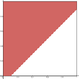
Figure 2. Region of the parameter space where the inequality holds. Parameters $b$ and $c$ vary over $X$ and $Y$ axis respectively. The value of $d$ is set to $0.1$.

Case 2: $b=0$
To tackle this case we will use two different (albeit similar) bases. These are

$$\mbox{\scalebox{1.2}{$\chi$}}_{K}(\sigma)=\prod_{j\in K}\frac{1+d}{2}\left(\frac{1-d}{1+d}+\sigma(j)\right)\text{ and }\mbox{\scalebox{1.2}{$\chi$}}^{\prime}_{K}(\sigma)=\prod_{j\in K}\frac{1+d}{2}\left(\frac{1-d}{1+d}-\sigma(j)\right).$$

Together their respective regions cover the entire $\left\{b=0\right\}$ cube, except for some points on the border $\left\{a=1\right\}\cup\left\{d=0\right\}$ where the positive rates assumption fails. ∎

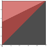
Figure 3. Regions of the parameter space where the criteria for these bases hold (black for the former, red for the latter). Parameters $a$ and $c$ vary over $X$ and $Y$ axis respectively. The value of $d$ is set to $0.01$. For $d>0.25$, the first base criterion fills the entire square.

One might be curious if the results now known are sufficient to prove that positive rates imply ergodicity in the case $\mathcal{A}=\left\{0,1\right\}$, $\mathcal{N}=\left\{0,1\right\}$, with no further restrictions. In the example above the problem was reduced by a dimension and solved in all cases except when $a=0$ and $b\geq c+d$. Unfortunately, our efforts fall short. Trying out different bases in Theorem 5.6 extends the covered region of parameters slightly, but there are points for which no product base will work. For example for $a=0$, $b=0.99$, $c=0.05$, $d=0.01$ there are no solutions in $A\in\mathbb{R}\setminus\left\{0\right\}$, $B\in\mathbb{R}$ to the inequality

$$\left|C_{\varnothing}\right|+C_{\left\{0\right\}}+\left|C_{\left\{1\right\}}\right|+\left|C_{\left\{0,1\right\}}\right|<1.$$

We have also experimented with making the product basis periodic, as in choosing different values for $\mbox{\scalebox{1.2}{$\chi$}}_{j}$ depending on the parity of $j\in\mathbb{Z}$, but that proved fruitless.

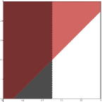
Figure 4. Using Theorem 5.6 with $A=1$ and $B\in[-1,0)$ one can additionally prove ergodicity for the cases $\left\{a=0,b<\frac{1}{2},c>0,d>0\right\}$, but our theorem is powerless in the neighborhood of $\text{IPS}(0,1,0,0)$. Parameters $b$ and $c$ vary over $X$ and $Y$ axis respectively. The value of $d$ is set to $0.1$.

That this method of proving ergodicity fails to cover the entire parameter space is not entirely surprising. Theorem 5.6 is blind to the structure of $\mathcal{G}$ and in particular does not take into account its dimension. There are no known counterexamples of "positive rates imply ergodicity" among nearest-neighbor IPS on $\mathbb{Z}$, but there are simple ones on $\mathbb{Z}^{2}$. A classic example is the Stochastic Ising Model - see chapter IV of Ligett’s textbook on IPS [Lig05]. Since dimension seems to be critical we should expect a proof that works on the entire parameter space to exploit the one-dimensionality of $\mathbb{Z}$ heavily.

We know of only one argument that proves ergodicity anywhere in the remaining region

$$\left\{a=0,b\approx 1,c\approx 0,d\approx 0\right\},$$

and it makes strong use of the dimension of $\mathbb{Z}$ - or rather of path crossing properties of a two-dimensional spacetime. It is the improved version of Gray’s theorem about monotone IPS i.e. Theorem 4.10.

Example 6.2.

A homogenous $\text{IPS}(P)$ on graph $\left(\mathbb{Z},\left\{0,1\right\}\right)$ with alphabet $\left\{0,1\right\}$ and parameters that satisfy $a\leq b<1$, $0<c\leq d$ is exponentially ergodic (c.f. Example 6.1 for definitions of $a$, $b$, $c$, $d$).

Proof of Example 6.2.

We will begin by sketching the strategy of the proof. The $\text{IPS}(P)$ is not itself weakly monotone. However, if we flip $0$s and $1$s at every other site the resulting $\text{IPS}(Q)$ will have a periodic transition matrix with the same parameters as $P$, just in a different order. While it may not be monotone (and in the case $a=0$ it cannot) the inequalities imposed to guarantee that it will be weakly monotone and have positive rates. Then by Theorem 4.10 this new $\text{IPS}(Q)$ will be exponentially ergodic. But of course, renaming states doesn’t change the underlying dynamics, so the original $\text{IPS}(P)$ must also be exponentially ergodic.

Formally the proof goes like this: Let $\zeta\in\text{IPS}(P)$ be a trajectory constructed as in Definition 2.9. We will define a modification of this trajectory

$$\xi_{t}(j)=\left\{\begin{array}[]{lc}\zeta_{t}(j),&j=0\left(\text{mod }2\right)\\ 1-\zeta_{t}(j),&j=1\left(\text{mod }2\right)\end{array}\right.\text{, for all }j\in\mathbb{Z}\text{ and }t\geq 0.$$

Clearly if $t\in\left[\tau_{n}^{j},\tau_{n+1}^{j}\right)$ then $\xi_{t}(j)=\xi_{\tau_{n}^{j}}(j)$ because $\zeta$ satisfies this condition and $\xi_{t}$ depends only on $\zeta_{t}$. Additionally $\xi$ evolves according to a transition matrix $Q$ given by

$$Q_{j}\left(z\;|\;x,y\right):=\mathbb{P}\left(\xi_{\tau_{n}^{j}}=z\;|\;\xi_{\tau_{n}^{j-}}(j,j+1)=(x,y)\right)=$$

$$\left\{\begin{array}[]{lc}\mathbb{P}\left(\zeta_{\tau_{n}^{j}}=z\;|\;\zeta_{\tau_{n}^{j-}}(j,j+1)=(x,1-y)\right),&j=0\left(\text{mod }2\right)\\ \mathbb{P}\left(\zeta_{\tau_{n}^{j}}=1-z\;|\;\zeta_{\tau_{n}^{j-}}(j,j+1)=(1-x,y)\right),&j=1\left(\text{mod }2\right)\end{array}\right.=$$

$$\left\{\begin{array}[]{lc}P_{j}\left(z\;|\;x,1-y\right),&j=0\left(\text{mod }2\right)\\ P_{j}\left(1-z\;|\;1-x,y\right),&j=1\left(\text{mod }2\right)\end{array}\right..$$

Thus $\xi$ is by Definition 2.10 a trajectory of $\text{IPS}(Q)$. The matrices $Q_{j}$ have parameters $(b,a,d,c)$ when $j$ is even and $(1-c,1-d,1-a,1-b)$ when $j$ is odd. Their weak monotonicity and positive rates are equivalent to the conditions we set. By Theorem 4.10 the $\text{IPS}(Q)$ is exponentially ergodic. Equivalently it has exponential covariance decay. But clearly, if covariances decay for trajectory $\xi$ then they decay at the same rate for trajectory $\zeta$, because for any $f\in F$ the function

$$\sigma\mapsto f\left(\left\{\begin{array}[]{lc}\sigma(j),&j=0\left(\text{mod }2\right)\\ 1-\sigma(j),&j=1\left(\text{mod }2\right)\end{array}\right.\right)$$

is also a member of $F$ (this transformation does not change $\text{Dom}(f)$). Thus $\text{IPS}(P)$ has exponential covariance decay. Equivalently it is exponentially ergodic. ∎

Figure 5. Union of regions in case $\left\{a=0\right\}$ for which we have a proof of ergodicity. The lower red bar is the region covered in Example 6.2. Parameters $b$ and $c$ vary over $X$ and $Y$ axis respectively. The value of $d$ is set to $0.1$.

We have been unable to prove ergodicity in the remaining region. However, simulations and heuristics suggest that this region should also be ergodic: If an IPS was not ergodic one would expect that by decreasing noise in its rule one would get another non-ergodic IPS. Meanwhile, the least noisy, deterministic IPS seem to be cut off from the remaining region.

7. Appendix

This appendix is not necessary to understand the overall picture of the article. We add it to provide clarity of claimed and cited results in Section 4. The complication comes from the use of different settings and notation, which would have obstructed the understanding of the main ideas. Each of the following subsections is written using the notation and constructions of the original works. We propose that before reading the subsequent sections readers familiarize themselves with the notation of the works referenced.

7.1. Addendum to Theorem 4.6

We mentioned that the theorem as written in Gray’s paper [Gra82] is slightly weaker than Theorem 4.6. The reason is that the rates-based construction used by Gray is less general than the one we employ. More precisely, it corresponds to the choice of the update function

$$f_{j}\left(\sigma,C\right)=\left\{\begin{array}[]{lr}\mathbbm{1}\left(C\geq\overline{\gamma}_{j}-\beta_{j}\left(\sigma\right)\right)&\sigma(j)=0\\ \mathbbm{1}\left(C\geq\delta_{j}\left(\sigma\right)\right)&\sigma(j)=1\end{array}\right.$$

where $\beta$s and $\delta$s are birth and death rates respectively and

$$\overline{\gamma}_{j}=\sup_{\sigma}\beta_{j}(\sigma)+\sup_{\sigma}\delta_{j}(\sigma).$$

This choice of update function imposes a restriction that the values of $P_{j}\left(1\;|\;\sigma\right)$ must be equal for at least two different $\sigma$s - the ones that maximize $\delta_{j}$ and $\beta_{j}$. This condition is not present in our construction. The theorem nevertheless holds because the exact same proof works for

$$g_{j}\left(\sigma,C\right)=\mathbbm{1}\left(C\geq P_{j}\left(0\;|\;\sigma\right)\right),$$

which permits all transition matrices. To see that the proof goes through notice that the construction of the edge processes $l_{t}^{m}$, $r_{t}^{m}$ can be copied exactly using the function $g$ and retain the properties $E1-E5$. That is because the only properties $g$ must satisfy is being non-decreasing in both $C$ and $\sigma$ and depending only on the nearest neighbors of $j$. Once we have these processes the rest of the proof doesn’t use the rates except in two instances. Firstly, the rates have to be positive and periodic (which corresponds to assuming that $P$ has positive rates and is periodic). Secondly, at a very technical moment near the end of the proof, $\beta^{*}$ must be replaced by $P_{\overline{x}}\left(1\;|\;\xi_{\sigma-}^{R_{m}}\right)$ or $P_{\overline{x}}\left(1\;|\;\xi_{\sigma-}^{L_{m}}\right)$ and the $\sigma$-algebra $\mathcal{F}\left(n^{\prime},x^{\prime},b\right)$ generated by all the variables $C_{n}(x),T_{n}(x)$ except $C_{n^{\prime}}(x^{\prime})$ and by event $\left\{C_{n^{\prime}}\left(x^{\prime}\right)\geq\overline{\gamma}_{x^{\prime}}-b\right\}$ needs to be generated by event $\left\{C_{n^{\prime}}\left(x^{\prime}\right)\geq 1-b\right\}$ instead.

7.2. Addendum to Theorem 4.11: Characterization of additive IPS

The notation of Griffeath’s construction can be found in the "percolation substructures" and "general construction" sections of [Gri78]. This construction permits IPS which updates many sites at once. The first thing we need to do then is to identify the choices of $V_{i,x}$ and $W_{i,x}$ for which only one site can updated at a time. It is easy to see that the possible choices for $V_{i,x}$ are

$$V_{i,x}=\varnothing\textit{ or }V_{i,x}=\left\{x\right\},$$

and the possible choices of $W_{i,x}$ are

$$W_{i,x}(y)=\left\{\begin{array}[]{lr}\left\{y\right\}&y\notin S_{x}\\ \left\{x,y\right\}&y\in S_{x}\end{array}\right.\text{ for any choice of }S_{x}\subseteq\mathcal{N}_{x}.$$

We will find it convenient to set the index family $I_{x}=\left\{0,1\right\}\times 2^{\mathcal{N}_{x}}$ and set

$$V_{0,S,x}=\varnothing\textit{, }V_{1,S,x}=\left\{x\right\}$$

and $W_{i,S,x}$ as above with $S_{x}=S$. Each pair $\left(V_{i,S,x},W_{i,S,x}\right)$ represents an update by a transition matrix $P_{i,S,x}$ with

$$P_{1,S,x}\left(1\,|\,\sigma\right)=1,$$

$$P_{0,S,x}\left(1\,|\,\sigma\right)=\left\{\begin{array}[]{lr}1&S\cap\sigma^{-1}\left(1\right)\neq\varnothing\\ 0&S\cap\sigma^{-1}\left(1\right)=\varnothing\end{array}\right..$$

For a given choice of $\lambda_{i,S,x}$ the transition matrix of IPS thus constructed is

$$P_{x}=\frac{1}{\lambda}\left[\left(\lambda-\lambda_{x}\right)I+\sum_{\begin{array}[]{l}i\in\left\{0,1\right\}\\ S\subseteq\mathcal{N}_{x}\end{array}}\lambda_{i,S,x}P_{i,S,x}\right]$$

where

$$\lambda_{x}=\sum_{\begin{array}[]{l}i\in\left\{0,1\right\}\\ S\subseteq\mathcal{N}_{x}\end{array}}\lambda_{i,S,x},$$

$$\lambda=\sup_{x\in\mathbb{Z}^{d}}\lambda_{x}.$$

The clock is $\text{Exp}\left(\lambda\right)$, but that can be normalised by rescaling all $\lambda_{i,S,x}$ by $\frac{1}{\lambda}$.

7.3. Addendum to Theorem 4.12: Characterization of cancellative IPS

Again the same pairs $\left(V_{i,S,x},W_{i,S,x}\right)$ are available for the construction. However, the transition matrices $P_{i,S,x}$ corresponding to them are different:

$$P_{0,S,x}\left(1\,|\,\sigma\right)=\left|S\cap\sigma^{-1}\left(1\right)\right|\left(\text{mod }2\right)$$

$$P_{1,S,x}\left(1\,|\,\sigma\right)=1-\left|S\cap\sigma^{-1}\left(1\right)\right|\left(\text{mod }2\right).$$

References

- [Gra82] Lawrence Gray. The positive rates problem for attractive nearest neighbor spin systems on z. Z. Wahrscheinlichkeitstheorie verw. Gebiete, 61:389–404, 1982.
- [Gra01] Lawrence Gray. A reader’s guide to gacs’s “positive rates” paper. Journal of Statistical Physics, 103:1–44, 2001.
- [Gri78] David Griffeath. Additive and cancellative interacting particle systems. Lecture Notes in Mathematics, 724, 1978.
- [Gá86] Peter Gács. Reliable computation with cellular automata. Journal of Computer and System Sciences, 32(1):15–78, 1986.
- [Lig05] Thomas Liggett. Interacting particle systems. Springer Berlin, Heidelberg, 2005.
- [TVS+90] A. Toom, N. Vasilyev, O. Stavskaya, L. Mityushin, G. Kurdyumov, and S. Pirogov. Discrete local markov systems. Manchester University Press, 1990.
- [VNLM70] Vaserstein, Leonid Nisonovich, Leontovich, and Aleksandr Mikhailovich. Invariant measures of certain markov operators describing a homogeneous random medium. Problemy Peredachi Informatsii, 6:71–80, 1970.