Nonlinear Expectation Inference for Direct Uncertainty Quantification of Nonlinear Inverse Problems

Abstract

Most existing inference methods for the uncertainty quantification of nonlinear inverse problems need repetitive runs of the forward model which is computationally expensive for high-dimensional problems, where the forward model is expensive and the inference need more iterations. These methods are generally based on the Bayes’ rule and implicitly assume that the probability distribution is unique, which is not the case for scenarios with Knightian uncertainty. In the current study, we assume that the probability distribution is uncertain, and establish a new inference method based on the nonlinear expectation theory for ’direct’ uncertainty quantification of nonlinear inverse problems. The uncertainty of random parameters is quantified using the sublinear expectation defined as the limits of an ensemble of linear expectations estimated on samples. Given noisy observed data, the posterior sublinear expectation is computed using posterior linear expectations with highest likelihoods. In contrary to iterative inference methods, the new nonlinear expectation inference method only needs forward model runs on the prior samples, while subsequent evaluations of linear and sublinear expectations requires no forward model runs, thus quantifying uncertainty directly which is more efficient than iterative inference methods. The new method is analysed and validated using 2D and 3D test cases of transient Darcy flows.

1 Introduction

The inference or inversion of uncertain parameters associated with governing partial differential equations (PDEs) is important and often inevitable in many physical and engineering problems (Kaipio and Somersalo, 2006; Oliver et al., 2008; Xiu, 2010; Smith, 2013). For scenarios where the parameters are known and certain, the governing PDEs can be solved numerically or approximated by surrogates to predict the dynamic responses (Zhang, 2022; Zhang et al., 2023). However, it is usually the case that one or more parameters of the governing PDEs are uncertain, and it is necessary to infer the parameters using observed data and prior knowledge of the dynamical system before reasonable predictions can be made (Caers, 2011; Yan and Guo, 2015; Arnold et al., 2019; Zhang et al., 2021).

Most existing methods for inferring uncertain parameters are based on the Bayes’ rule, where the posterior probability density function (pdf) is evaluated using the prior and likelihood pdfs (Stuart, 2010). These methods are either for a point-estimate or an approximation of the true posterior pdf. Point-estimate methods mainly include gradient-based approaches (e.g. stochastic gradient descent, Newton and quasi-Newton methods) and heuristic algorithms (e.g. evolution and simulated annealing) (Ma et al., 2020; Yan and Zhou, 2021). These methods aim at obtaining the maximum a posterior (MAP) or the maximum likelihood estimate (MLE), where the latter is used with uniform or unknown prior. On the other hand, methods to approximate the true posterior pdf mainly include Markov Chain Monte Carlo (MCMC), variational Bayes and ensemble-based methods (e.g. ensemble Kalman filter and ensemble smoother) (Olalotiti-Lawal and Datta-Gupta, 2018; Emerick and Reynolds, 2013; Song et al., 2021; Povala et al., 2022). These methods approximate the posterior pdf using sample distributions, in the case of MCMC and ensemble-based methods, or trial functions in the case of variational Bayes.

For linear Gaussian inverse problems, analytical solutions exist for Kalman filter and variational Bayes (Emerick and Reynolds, 2013; Povala et al., 2022). For nonlinear and/or non-Gaussian inverse problems, almost all existing methods approximate the posterior (MAP, MLE or pdf) via updating the parameters iteratively, where forward simulation runs are needed in each iteration to evaluate the objective function. This can be highly expensive, especially for high-dimensional nonlinear inverse problems where forward simulation is expensive and parameter optimization requires a large number of iterations. Therefore, it is very important to develop efficient uncertainty quantification methods for high-dimensional nonlinear inverse problems.

Conventional inference methods based on the Bayes’ rule are built in the classic Kolmogorov probability space. In the classic probability space, the probability distribution is certain and the expectations can be added linearly. However, linear additivity is no longer the case if the probability distribution itself is uncertain or unknown, which is true in many practical problems. The uncertainty of probability distribution itself is referred to as Knightian uncertainty, model uncertainty or ambiguity. To account for Knightian uncertainty, Choquet (1954) extended the Lebesgue integration concept to non-additive measure to obtain a nonlinear expectation, which is however not dynamically consistent (Peng, 2019). Peng (1997) established dynamically consistent nonlinear expectations (g-expectation) in infinite-dimensional linear Wiener space. Further, the nonlinear expectation space is defined and the nonlinear expectation (G-expectation) theoretical framework is developed (Peng, 2004, 2017, 2019). In the nonlinear expectation theory, it is assumed that the stochastic process in most practical cases is of complex nature that no single distribution can serve as a perfect model, but should be described by a family of different distributions. The number of distributions in the family can be infinite while explicit formulations of the distributions are not to be expected. The nonlinear expectation theory has been applied successfully in data analysis to account for distribution uncertainty (Jin and Peng, 2021; Ji et al., 2023; Peng et al., 2023).

In the current study, we develop a direct inference method for the uncertainty quantification of nonlinear inverse problems based on the nonlinear expectation theory. Given prior samples, no explicit probability distribution is assumed. Instead, we assume a sublinear expectation space for the uncertain probability distribution characterized by the maximum of linear expectations. Given observed data, posterior linear expectations are obtained by choosing those associated with higher likelihood. Since the computation of linear expectations involves no forward model runs, it can be done very efficiently. Then the uncertainty of inference is quantified by the sublinear expectation computed using the posterior linear expectations.

The paper is organised as follows. In section 2, the uncertainty quantification problem for random parameters associated with PDEs are introduced. In section 3, the new nonlinear expectation inference (NEI) method is developed. In section 4, NEI is validated on 2D and 3D test cases of transient Darcy flows. Section 5 is the conclusion of the paper.

2 The Uncertainty Quantification Problem

2.1 General Forward Model

In the current study, we focus on the uncertainty quantification of random parameters associated with PDEs governing physical processes. Let $m\in\mathcal{M}$ be the random parameter and $d\in\mathcal{D}$ be the observations of solution, where $\mathcal{M}$ and $\mathcal{D}$ are Banach spaces, we have in compact form

$$d=\mathcal{G}(m)+\epsilon~{},$$ (1)

where $\mathcal{G}$ is the mapping from $\mathcal{M}$ to $\mathcal{D}$, and $\epsilon$ is additive observation noise. Let $\mathcal{A}:\mathcal{M}\rightarrow\mathcal{U}$ be a solution operator of the governing PDE, where $\mathcal{U}$ is a Hilbert space, and $\mathcal{P}:\mathcal{U}\rightarrow\mathcal{D}$ be a projection operator, Eq. (1) can be written as

$$d=\mathcal{P}(\mathcal{A}(m))+\epsilon~{}.$$ (2)

2.2 The Inverse Problem and Bayesian Uncertainty Quantification

The inverse problem is to estimate the random parameter $m$ given the observations $d$. The first Bayesian approach is to build the inference model in the function space before discretizing the model, e.g. the pre-conditioned Crank-Nicholson MCMC scheme (Cotter et al., 2013; Pinski et al., 2015). The second and widely used Bayesian approach is to build the inference model in the finite-dimensional space after discretizing the forward model, where the random parameter $m$ can be estimated using Bayes’ rule as

$$p(m|d)=\frac{p(d|m)p(m)}{\int p(d|m)p(m)dm}\propto p(d|m)p(m)~{},$$ (3)

where $p(m|d)$ is the posterior, $p(d|m)$ is the likelihood and $p(m)$ is the prior pdf. The likelihood is evaluated using the forward model given the pdf of observation noise.

For nonlinear inverse problems, analytical solutions of the posterior pdf are generally not available and iterative inference methods need to be used. Existing iterative inference algorithms are either to find a point-estimate or to approximate the posterior pdf itself. The former mainly includes gradient-based, heuristic and data assimilation methods for computing the maximum a posterior (MAP) or maximum likelihood estimate (MLE), while the latter includes MCMC and variational Bayes approaches (Posselt, 2013; Emerick and Reynolds, 2013; Povala et al., 2022). All these methods need repetitive evaluations of the forward model in the inference process, which can be computationally expensive for high-dimensional problems.

3 Nonlinear Expectation Inference

While the classic probability theory is for probability measures that are (approximately) certain, the nonlinear expectation theory is for probability measures that are uncertain. In this section, we introduce our new method, called nonlinear expectation inference (NEI), based on the nonlinear expectation theory which is a powerful framework to deal with problems with Knightian uncertainty. A typical example of nonlinear expectation is a sublinear expectation (SLE) (Peng, 2019; Guo and Li, 2021), denoted by $\hat{E}$ and defined as the upper expectation over a set of probability measures $\mathcal{P}$, i.e.,

$$\hat{E}[X]=\sup_{P\in\mathcal{P}}E_{P}[X]~{},$$ (4)

where $\mathcal{P}$ is a set of probability measures on measurable space $(\Omega,\mathcal{F})$ characterizing Knightian uncertainty, and $E_{P}[\cdot]$ is the linear expectation introduced by $P\in\mathcal{P}$. $\hat{E}[X]$ is sublinear as $\hat{E}[X+Y]\leq\hat{E}[X]+\hat{E}[Y]$. The corresponding lower expectation can be obtained as $-\hat{E}[-X]=\inf_{P\in\mathcal{P}}E_{P}[X]$.

Precisely, we consider the inverse problem of inferring $m$ given observed $d$ associated with a forward model

$$d=\mathcal{\psi}(m)+\epsilon~{}.$$ (5)

where $m$, $d$ and $\epsilon$ are all vectors, and $\psi$ can be approximated by numerical simulation. The classical assumption is that the probability distribution of $\epsilon$ is known while that of $m$ is unique but with unknown parameters. Here, we assume that the distribution of $m$ is not unique and aim to infer $m$ given $d$ and a number of prior samples. The nonlinear expectation inference (NEI) method is developed as follows.

(1) Estimate the Prior Uncertainty

Let $\mathcal{M}=\{m_{i},1\leq i\leq n\}$ denote the set containing $n$ prior samples, and $\mathcal{P}$ the set of the all possible probability distributions for $m$. Enlightened by the $\psi$-max-mean algorithm (Peng, 2019), $\mathcal{P}$ is built to contain linear expectations approximated by sample distributions, where a sample distribution is a subset of $\mathcal{M}$. The total number of subsets of $\mathcal{M}$ is $2^{n}$. Since $n>>1$, we have $2^{n}>>n$.

Practically, evaluating linear expectations on a total number of $2^{n}$ subsets may be too expensive, and we can use a limited number of subsets for estimation. Suppose $K$ subsets are built, $\mathcal{P}$ contains $K$ linear expectations defined on the subsets accordingly. The prior uncertainty of $m$ can be quantified using the upper and lower expectations $\bar{\psi}=\hat{E}[\psi(m)]$ and $\underline{\psi}=-\hat{E}[-\psi(m)]$ such that

$$\hat{E}[\psi(m)]=\max_{j=1,\dots,K}E_{M_{j}}[\psi(m)],$$ (6)

where $E_{M_{j}}[\psi(m)]$ is evaluated on subset $M_{j}=\{m_{j1},\dots,m_{jk}\}\subseteq\mathcal{M}$ as $E_{M_{j}}[\psi(m)]=\frac{1}{k}\sum_{i=1}^{k}\psi(m_{ji})$

The true $\psi(m)$ is bounded by $\bar{\psi}$ and $\underline{\psi}$ given sufficient prior samples. In the sublinear expectation theory, two random variables $X$ and $Y$ with uncertain probability distributions are identical if $\hat{E}[\psi(X)]=\hat{E}[\psi(Y)]$ for all $\psi$. Here, $\bar{\psi}$ and $\underline{\psi}$ are the reflection of the distribution uncertainty of $m$ on $\psi$.

(2) Estimate the Posterior Uncertainty

Given a specific observed $d_{obs}$ and the likelihood function $L$ (e.g. multivariate Gaussian), conventionally the likelihood of a sample (realisation) $m_{i}$ can be evaluated using $L(d_{sim},d_{obs})$ where $d_{sim}=\psi(m_{i})$. Here, we compute the likelihood $L_{j}$ for each subset $M_{j}$ with linear expectation $E_{M_{j}}[\psi(m)]$ as

$$L_{j}=L(E_{M_{j}}[\psi(m)],d_{obs})~{}.$$ (7)

Let $\mathcal{M}_{K}=\{M_{j},1\leq j\leq K\}$ denote the set of $K$ subsets. The posterior subsets $M^{*}_{j}$ ($j=1,\dots,K^{*}$ and $K^{*}<K$) are obtained using the MLE principle by choosing from $\mathcal{M}_{K}$ a number of $K^{*}$ subsets with highest likelihoods. Here, $*$ marks posterior. Denote $\mathcal{M}^{*}_{K^{*}}=\{M^{*}_{j},1\leq j\leq K^{*}\}$ be the set of all posterior subsets, we have

$$\min_{M^{*}_{j}\in\mathcal{M}^{*}_{K}}L(E_{M^{*}_{j}}[\psi(m)],d_{obs})\geq\max_{M_{j}\in\mathcal{M}_{K}\setminus\mathcal{M}^{*}_{K^{*}}}L(E_{M_{j}}[\psi(m)],d_{obs})~{}.$$ (8)

The posterior subsets are used to estimate the posterior upper and lower expectations $\bar{\psi}^{*}=\hat{E}^{*}[\psi(m)]$ and $\underline{\psi}^{*}=-\hat{E}^{*}[-\psi(m)]$ as

$$\hat{E}^{*}[\psi(m)]=\max_{j=1,\dots,K^{*}}E_{M^{*}_{j}}[\psi(m)],$$ (9)

where $E_{M^{*}_{j}}[\psi(m)]$ is introduced by $M^{*}_{j}$, $1\leq j\leq K^{*}$. Therefore, the inference results are the posterior subsets (sample distributions) on which the estimated linear expectations $\hat{E}^{*}[\psi(m)]$ are of highest likelihoods. The algorithm of NEI is summarised in Algorithm 1.

Algorithm 1 Nonlinear Expectation Inference for Inverse Problems

0:  Prior sample set $\mathcal{M}=\{m_{i},1\leq i\leq n\}$, observed data vector $d$, the likelihood function $L$ and the forward model $\psi$.

0:  Posterior SLE, associated linear expectations and subsets.

1:  Run forward model on all prior samples to obtain the dynamic response $u_{i}=\psi(m_{i})$ for each sample.

2:  Build a number of $K$ subsets of $\mathcal{M}$.

3:  Evaluate the linear expectations of $\psi(m_{i})$ on the sample distributions defined by the subsets as $E_{M_{j}}[\psi(m)]=\frac{1}{k}\sum_{i=1}^{k}\psi(m_{ji})$, where $m_{ji}$ is the $i^{\prime}$th sample in the $j^{\prime}$th subset.

4:  Calculate the prior upper $\bar{\psi}=\hat{E}[\psi(m)]$ and lower expectation $\underline{\psi}=-\hat{E}[-\psi(m)]$ according to Eq. (6). The observation $d$ should be bounded by $\bar{\psi}$ and $\underline{\psi}$. If not, introduce more prior samples until the condition is true.

5:  Evaluate the likelihood $L_{j}$ for the linear expectation associated with the $j^{\prime}$th subset.

6:  Obtain a number of $K^{*}$ linear expectations with highest likelihoods and their related subsets. Each linear expectation $E_{M_{j}}[\psi(m)]$ characterises a probability model for $m$.

7:  The posterior upper and lower expectations $\bar{\psi}^{*}=\hat{E}^{*}[\psi(m)]$ and $\underline{\psi}^{*}=-\hat{E}^{*}[-\psi(m)]$ are computed as Eq. (9) to quantify the posterior Knightian uncertainty of $m$.

8:  The Knightian uncertainty of $m$ is represented by the expectations on posterior subsets regarded as sample distributions. For prediction, the samples in the union of posterior subsets are simulated further, and the corresponding linear expectations are computed to yield the SLEs for prediction.

The convergence of NEI is proved simply as follows. Since the set of posterior subsets is contained in the set of prior subsets, the set of posterior samples is contained in the set of prior samples. In consequence,

$$\hat{E}^{*}[\psi(m)] \leq \hat{E}[\psi(m)]~{},$$ (10)

$$\hat{E}^{*}[-\psi(m)] \leq \hat{E}[-\psi(m)]~{}.$$ (11)

Therefore, we have

$$\bar{\psi}^{*} \leq \bar{\psi}~{},$$ (12)

$$\underline{\psi}^{*} \geq \underline{\psi}~{}.$$ (13)

which means that the posterior $m$ has a lower uncertainty than the prior $m$, and the inference converges towards higher likelihood because of Eq. (8).

The NEI method is highly log as we only need to conduct forward model runs on prior samples, and the evaluation of linear expectations on subsets are directly on the solutions with no further forward model runs. Therefore, the uncertainty quantification via NEI is called direct, to distinguish itself from the existing iterative inference algorithms that need repetitive runs of the forward model.

The value of $K^{*}$ is flexible. To be comparable to existing ensemble-based methods, we can set $K^{*}=n<<K$. In many practical cases, the aim of parameter inference or inversion is to predict with higher accuracy. For prediction with NEI, forward model runs are conducted on samples in $\underset{j=1,...,K^{*}}{\cup}M^{*}_{j}\subseteq\mathcal{M}$. Then the predicted results are used to compute the linear expectations on posterior subsets, and the uncertainty is quantified by SLE calculated by Eq. (9).

4 Test Cases

The test cases in the current study are to infer the uncertain permeability fields as parameters of the governing PDE for transient Darcy flow given observed flow rates. No explicit $\psi$ is available, while $\psi$ represents the nonlinear mapping from the permeability field to the flow rates which can be approximated by numerical simulation.

4.1 The Governing Equation for Transient Darcy Flow

The governing PDE for transient single-phase slightly compressible Darcy flows is

$$\phi c_{t}\frac{\partial p}{\partial t}=\nabla\cdot(\frac{K}{\mu}\nabla p)+f~{},$$ (14)

where $p=p(\textbf{x},t)$ is pressure, $K=K(\textbf{x})$ is permeability, $c_{t}$ is total compressibility, $\mu$ is viscosity, $\phi=\phi(\textbf{x})$ is porosity, $f=f(\textbf{x})$ is the source/sink term, $t$ is time and x is the spatial coordinate. The finite volume method with implicit time integration (Chen et al., 2006) can be adopted for solving Eq. (14) numerically as

$$V_{i}\phi C_{t}\frac{p_{i}^{n+1}-p_{i}^{n}}{\Delta t}=\sum_{j}T_{ij}(p_{j}^{n+1}-p_{i}^{n+1})+q_{i}^{n}~{},$$ (15)

where $V_{i}$ is the volume of the $i$’th grid cell, $p_{i}^{n}$ is the pressure at the $i$’th cell and time step $n$. $q_{i}=fV_{i}$ is the volumetric source or sink term. $T_{ij}$ is the transmissibility between two neighbouring cells evaluated by harmonic average as

$$T_{ij}=(T_{i}^{-1}+T_{j}^{-1})^{-1}~{},$$ (16)

where $T_{i}$ is the transmissibility inside cell $i$ towards $j$ calculated as

$$T_{i}=\frac{K_{i}A_{ij}}{\mu d_{i}}~{},$$ (17)

where $A_{ij}$ is the area of the boundary face between cells $i$ and $j$, while $d_{i}$ is the distance from the cell centre to the face centre. The flow rate $q_{i}^{n}$ is evaluated at cells with non-zero sink term by

$$q_{i}^{n}=\text{PI}*(p_{i}^{n}-p_{wf})$$ (18)

where PI is the production index (Peaceman, 1978) and $p_{wf}$ is the constant bottom-hole pressure.

For the forward model Eq. (5), the uncertain parameter $m$ is $K$, the observed $d$ is the observed flow rates $q_{i}^{n}$ for all time steps $n$ and all cells $i$ with non-zero source or sink terms, and $\psi$ is the mapping from $m$ to $d$ approximated by the discretisation scheme Eq. (15)-(18).

4.2 Test Case 1: 2D Nonlinear Inverse Problem

The first example is the inversion of a 2D 10$\times$10 permeability field $k=k(x,y)$ given the observed flow rate (sink term). The permeability field is heterogeneous, isotropic and uncertain. All other parameters are constant shown in Table 1. A total of 50 prior samples (realisations) for the permeability field are built via conducting sequential Gaussian simulation (SGS) using the Stanford Geostatstical Modeling Software (SGeMS) (Remy et al., 2009) for $h=log_{2}(10k)$ where the unit of permeability $k$ is mD. The ground truth of the permeability field for generating the synthetic observation data is presented in Fig. 1(a). All boundaries are with no-flow condition while the flow is driven by the transient sink term at a corner. The pressure field at end of simulation using the true permeability field is shown in Fig. 1(b). For forward simulation, there are 180 time steps with $dt=100$k seconds. The noise in observation data is assumed to follow a multivariate Gaussian distribution $\mathcal{N}(0,C_{D})$ such that the likelihood follows $\mathcal{N}(g(m),C_{D})$. The covariance matrix $C_{D}$ of noise is assumed to be diagonal with constant entry $\sigma_{ob}=2\times 10^{-6}$ m³/sec equal to around 1.7% of the initial flow rate.

NEI and ensemble smoother multiple data assimilation (ESMDA) (Emerick and Reynolds, 2013) are conducted to inverse the permeability field for comparison. ESMDA is a highly log method that is widely used for parameter inversion of underground Darcy flows.

For NEI, we conduct forward simulation on the 50 prior samples, while no further forward runs are needed in the inversion process. Let each subset (ensemble or group of samples) contain no more than three samples, a total of $\sum_{i=1}^{3}C_{50}^{i}=20875$ subsets are built to compute the linear expectations $E_{i}(\vec{q})$, $i=1,...,20875$. Then the fifty subsets with highest likelihood are selected to be the posterior subsets. There are in total 25 non-repetitive samples inside the union of posterior subsets. For prediction using NEI, the 25 samples are simulated for a further period and the the corresponding linear expectations of flow rates on posterior subsets are computed. Then the sublinear upper and lower expectations are simply the upper and lower bounds of the expected flow rates.

For ESMDA, $h$ is inverted to recover $k$ according to $h=log_{2}(10k)$, as the distribution of $h$ is close to Gaussian. The ensemble of 50 samples are updated for six iterations until convergence to yield the posterior samples. For prediction using ESMDA, all 50 posterior samples are simulated.

The inference results of NEI and ESMDA are very close, as can be seen from Fig. 2 presenting the flow rates simulated using prior and posterior samples/subsets. The posterior flow rates of NEI is the linear expectations on posterior subsets. Here, simulation results of prior samples are used directly as the prior uncertainty to be comparable to conventional methods, e.g. ESMDA.

The negative log-likelihood of posterior samples by ESMDA and subsets by NEI are compared in Fig. 3 which implies that the inference results using NEI is slightly more accurate evaluated by likelihood. In addition, NEI is computational more log using 50 forward simulation runs while ESMDA needs an extra 300 forward runs. The cpu time for ESMDA is about 26 seconds, and that for NEI is about 6 seconds, where 2.5 seconds is for forward simulation and 3.5 seconds is for computing the linear expectations on subsets. The computation of all test cases are on a normal desktop computer with i9 cpu.

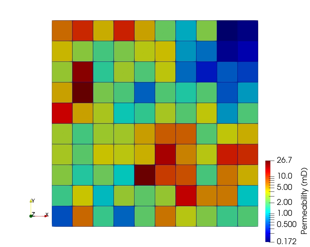
(a)

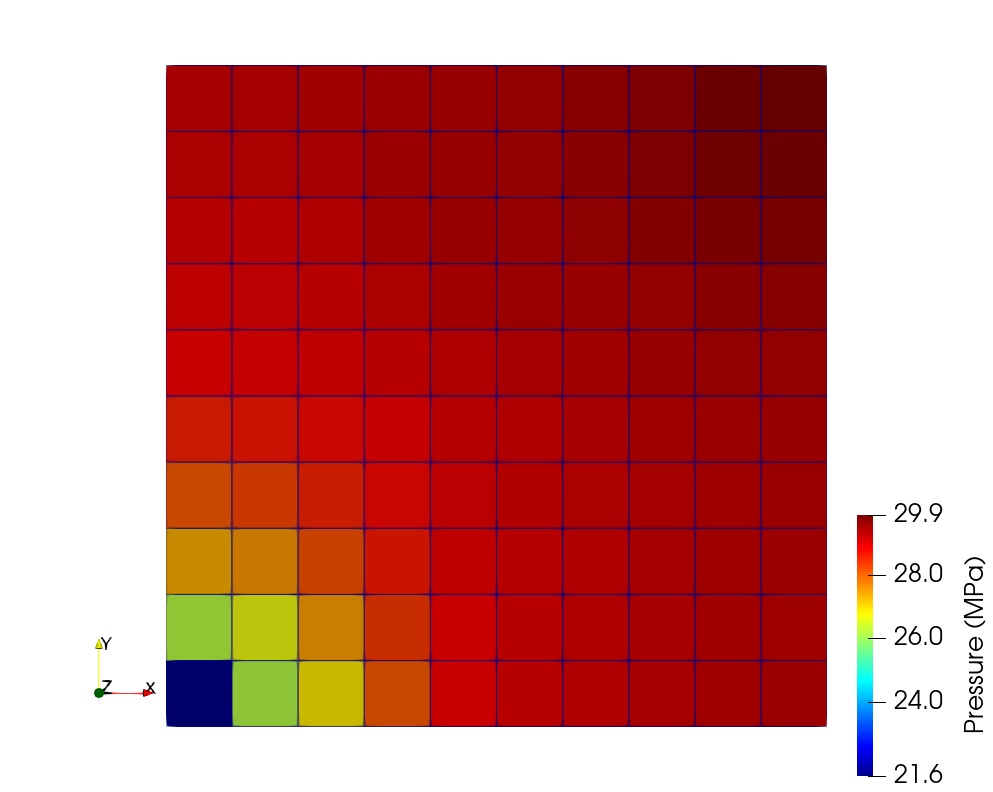
(b)

Figure 1: The ground truth for generating the observed flow rate data (a). The pressure field at end of simulation using the true permeability field (b).

Porosity	10%
Total Compressibility	$5\times 10^{-8}$ Pa-1
Dynamic Viscosity	0.002 Pa*s
Production Index	1.175$\times$10-5 m3Sec-1MPa-1
Bottom-hole Pressure	20 MPa

Table 1: A summary of constant physical and well parameters for the 2D model.

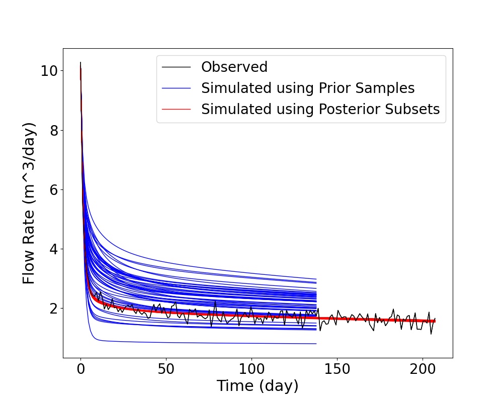
(a)

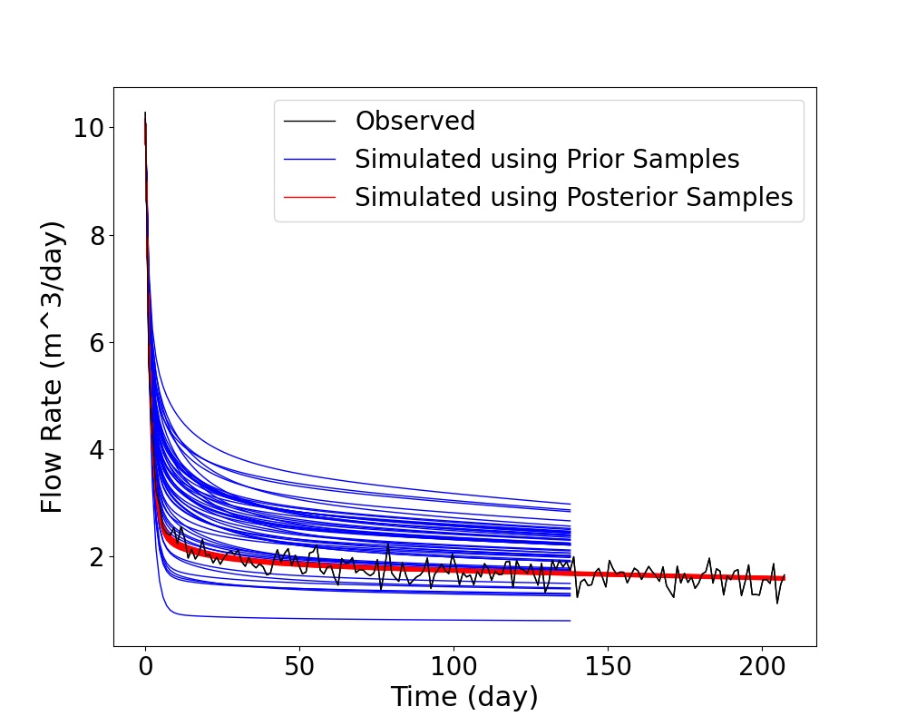
(b)

Figure 2: The predicted flow rate at wells using posterior subsets by NEI (a). The predicted flow rate at wells using posterior samples by ESMDA (b).

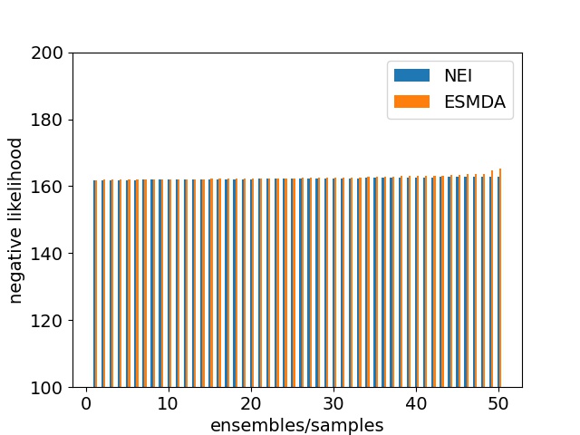
Figure 3: Comparison of the negative log-likelihood on posterior subsets/samples using NEI and ESMDA.

4.3 Test Case 2: 3D Nonlinear Inverse Problem

The second example is the inversion of a 3D 20$\times$20$\times$5 permeability field $k=k(x,y,z)$ given the observed flow rate. A total of 100 prior realisations are generated by SGS for $h=log_{2}(10k)$ where the unit of permeability $k$ is mD. All other parameters are as in Table 1 but with four wells of the same bottom-hole pressure at all corners of the reservoir model. The ground truth for the permeability field and the pressure field at end of simulation are shown in Figs. 4(a) and 4(b), respectively. For forward simulation, there are 150 time steps with $dt=100$ hours.

For NEI, we only need to conduct forward simulations on the 100 prior samples. Let each subset contain no more than three samples, the linear expectations on $\sum_{i=1}^{3}C_{100}^{i}=166750$ subsets are evaluated. Then, the 100 subsets with highest likelihood form the posterior subsets containing 38 non-repetitive samples which are simulated further for prediction. For ESMDA, the samples are updated for 5 iterations that needs an extra 500 forward model runs. The inference and predicted flow rates using NEI and ESMDA are shown in Figs. 5 and 6, respectively. The likelihood of the inference results by ESMDA is higher, and the predicted flow rates have a lower level of uncertainty. For NEI, the linear expectations of more subsets (e.g. the subsets containing four samples) can be evaluated to yield posterior subsets of higher likelihoods and a lower uncertainty. Yet, a higher uncertainty level is not necessarily worse, especially when it covers the fluctuating observed data and is more robust.

The computational cost for NEI is about 10 min, where 8 min is for 100 forward simulation runs on prior samples, and 2 min is for evaluating the linear expectations on subsets. The computational cost for ESMDA is about 48 min for 600 forward simulation runs.

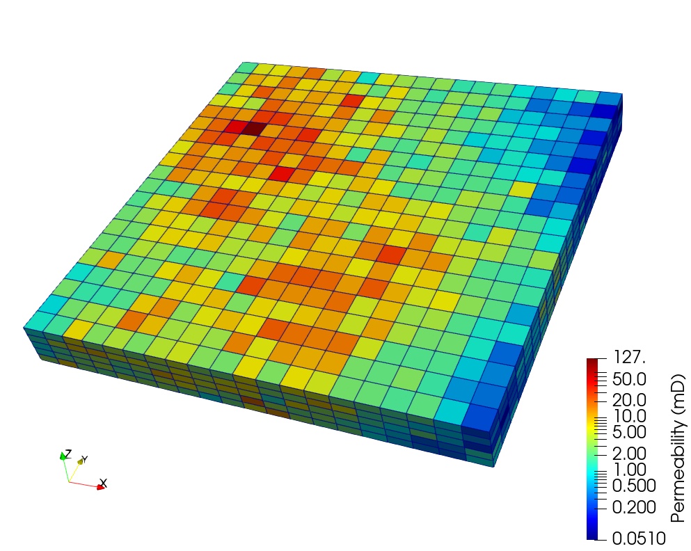
(a)

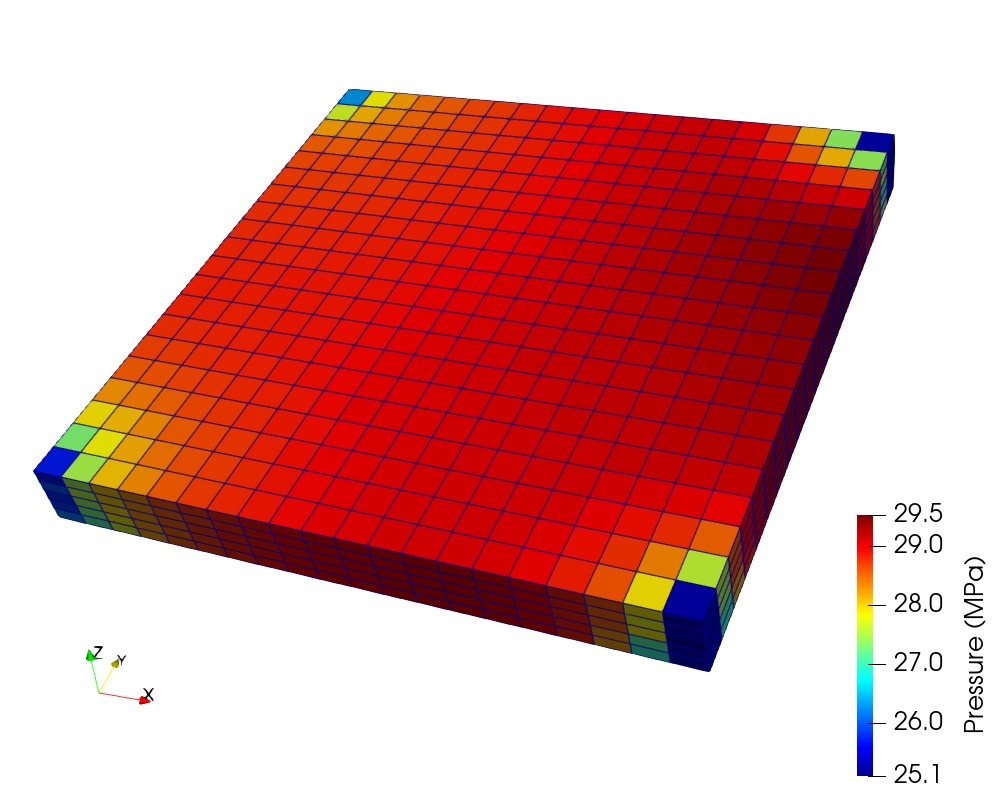
(b)

Figure 4: The ground truth for generating the observed flow rate data (a). The pressure field at end of simulation using the true permeability field (b).

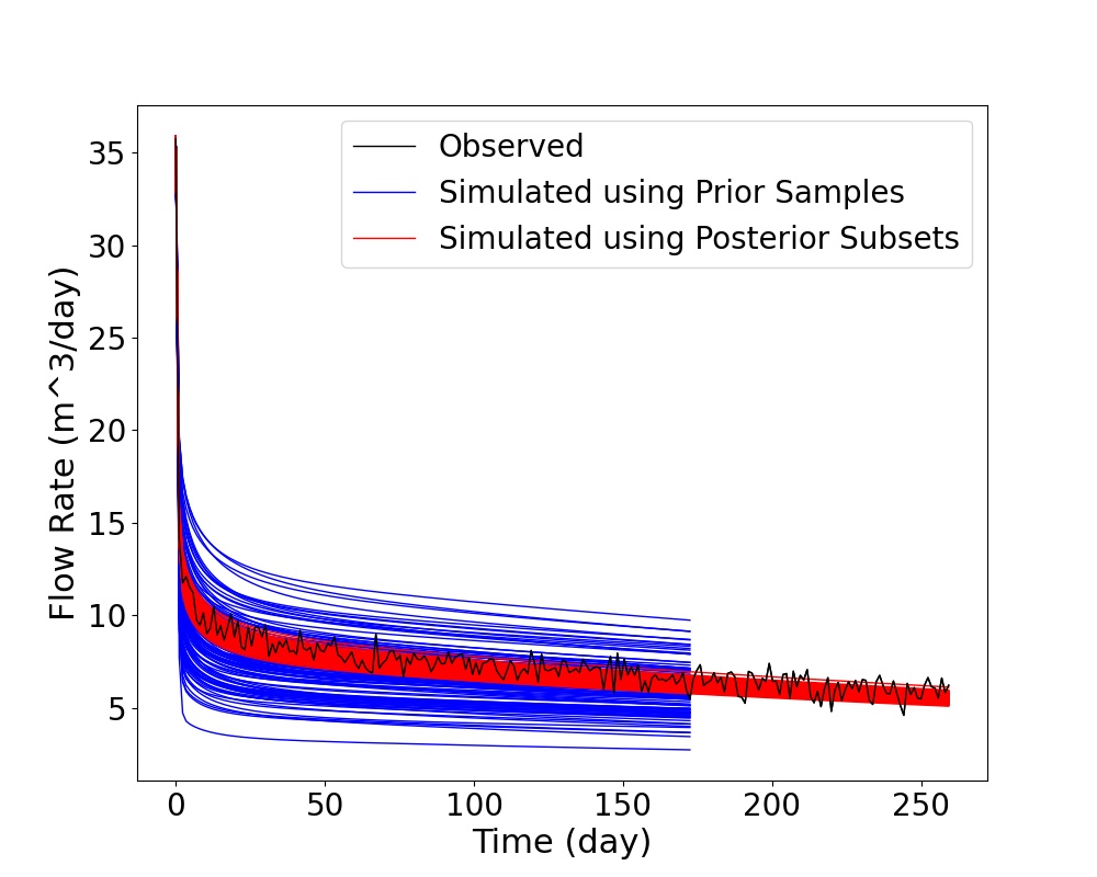
(a)

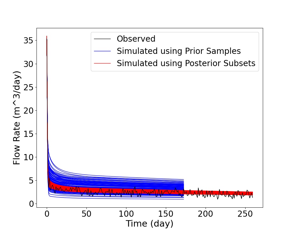
(b)

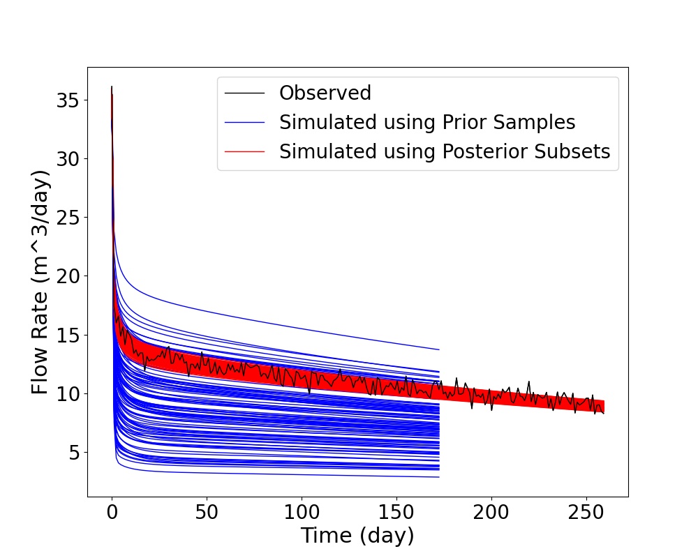
(c)

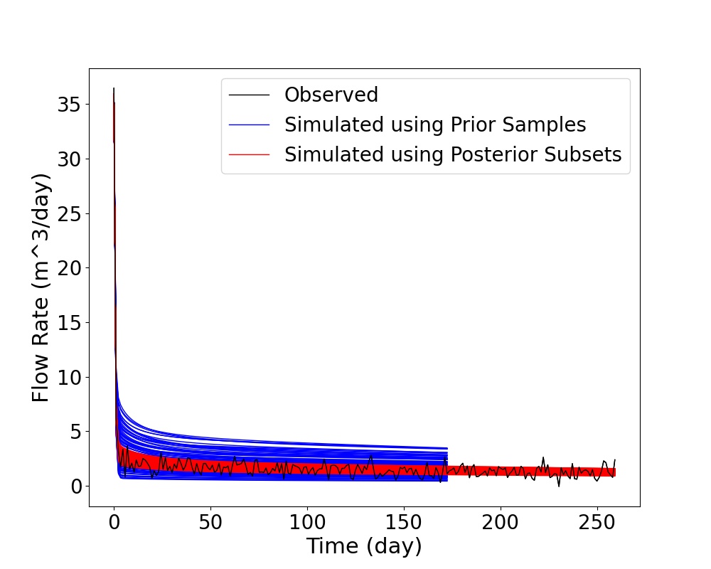
(d)

Figure 5: The simulated flow rates at wells using prior samples and posterior subsets by NEI for the 3D nonlinear inverse problem of transient Darcy flow.

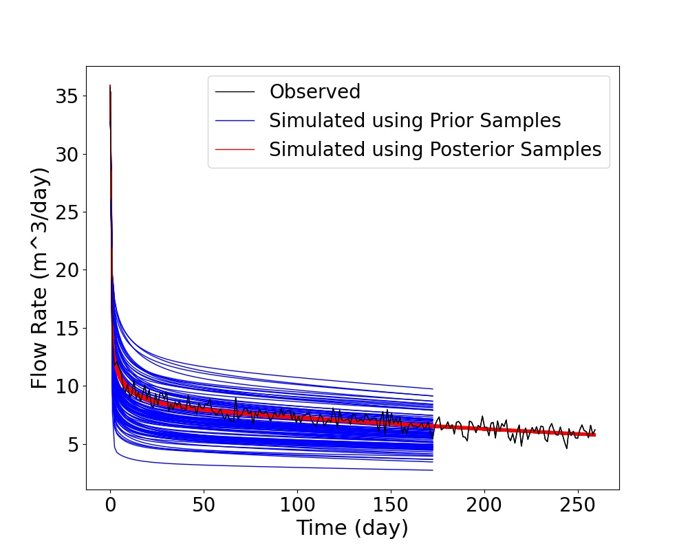
(a)

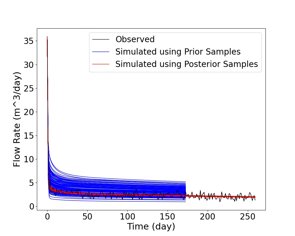
(b)

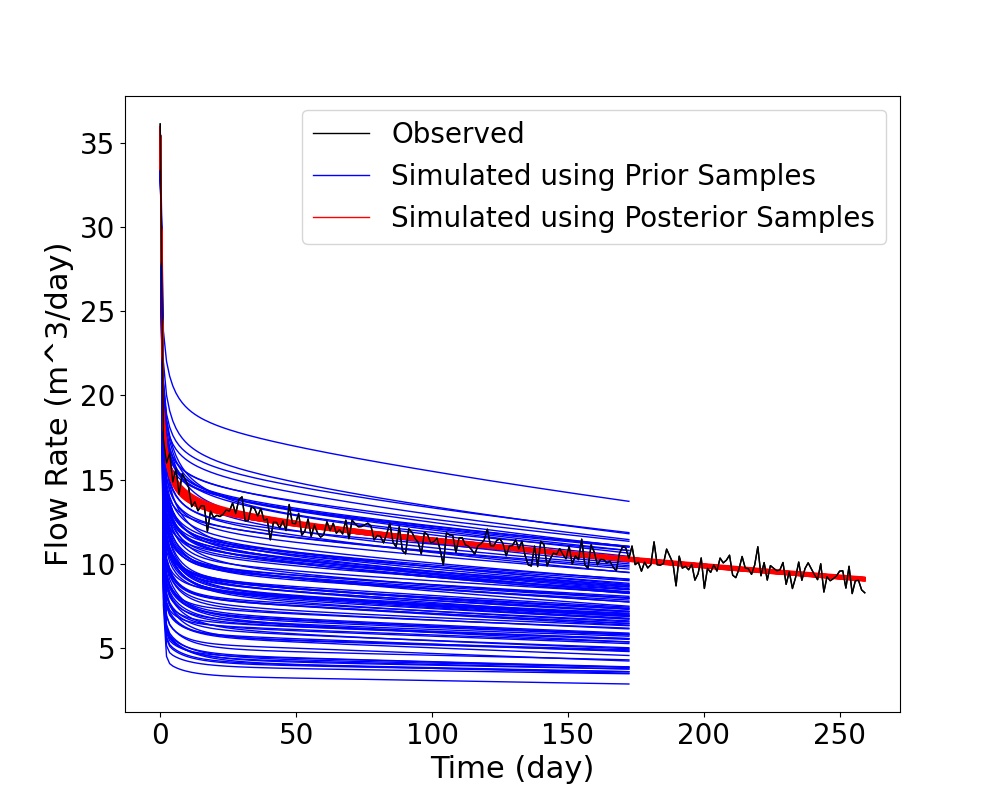
(c)

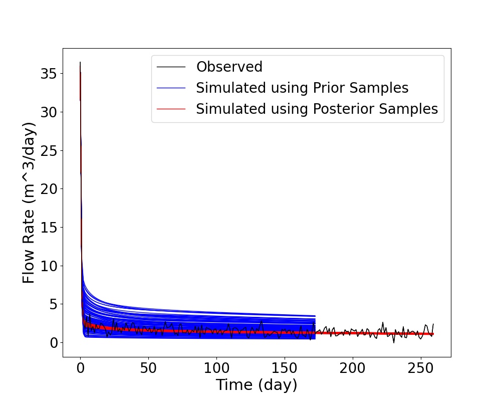
(d)

Figure 6: The simulated flow rates at wells using prior and posterior samples by ESMDA for the 3D nonlinear inverse problem of transient Darcy flow.

4.4 Test Case 3: 3D Non-Gaussian Nonlinear Inverse Problem

The third example is the inversion of the permeability field of the EGG reservoir model (Jansen et al., 2014). The EGG model is a synthetic channelized reservoir model consisting of 101 realisations considered to be geologically meaningful. One of the realisations is used as the ground truth, while all others serve as the prior models. The permeability distribution of the EGG model is non-Gaussian. There are in total 60$\times$60$\times$7 grid cells which are all active in the current study. The initial condition is that all cells are of pressure 30 MPa. There are four wells in the reservoir producing at the same bottom-hole pressure 26 MPa. The ground truth for the permeability field for generating the synthetic ’observed’ flow rates at the wells is shown in Fig. 7(a). The pressure field at the end of simulation is visualised in Fig. 7(b). For forward simulation, there are 72 time steps with $dt=5$k seconds. Two of the prior realisations are shown in Fig. 8 where the main characteristics of the reservoir are kept but the channels are of different location and shapes.

For NEI, we run forward simulations on the 100 prior models. Let each subset contain no more than three samples, a total of $\sum_{i=1}^{3}C_{100}^{i}=166750$ subsets are built and evaluated to yield 100 posterior subsets. Flow rates simulated using prior samples and posterior subsets are shown in Fig. 9. Since there are 32 samples in the union of the posterior subsets, we only need to simulate the 32 samples for prediction. The computational cost of NEI is around 16 hours for simulating the 100 prior samples plus 1 minute for evaluating linear expectations on the subsets. The sublinear upper and lower expectations are the bounds of the predicted flow rates quantifying the uncertainty of prediction.

The uncertainty is reduced by assuming no more than four samples in a subset and evaluate linear expectations on $\sum_{i=1}^{4}C_{100}^{i}=4087975$ subsets to yield the posterior subsets. The predicted flow rates are presented in Fig. 10. The interval between the upper and lower expected flow rates is reduced. The union of posterior subsets contain 31 samples meaning that the computational cost of prediction is not increased. For NEI with 4087975 subsets, the cost of evaluating linear expectations is increased to 27 minutes. On the other hand, it is challenging for ESMDA to converge for the inversion of the non-Gaussian permeability field in the current study.

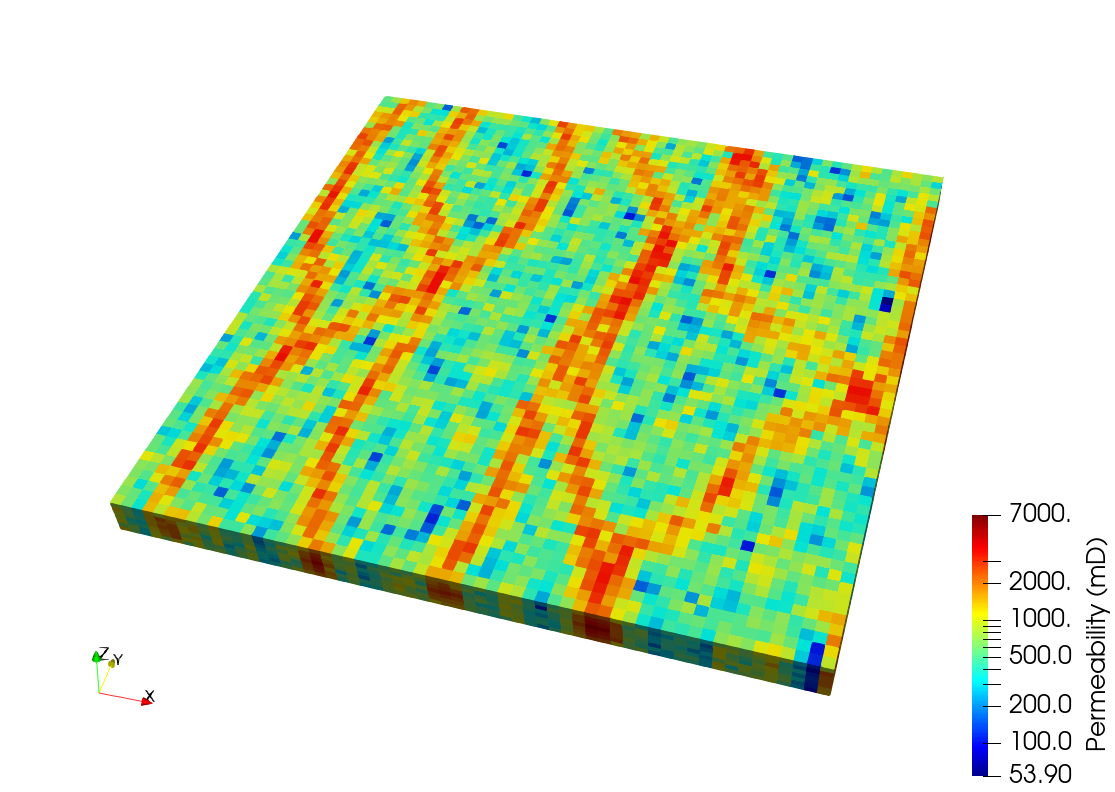
(a)

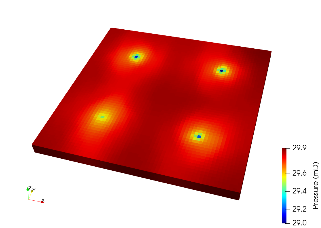
(b)

Figure 7: The ground truth for the permeability field of the EGG reservoir model (a). The pressure field at the end of simulation (b).

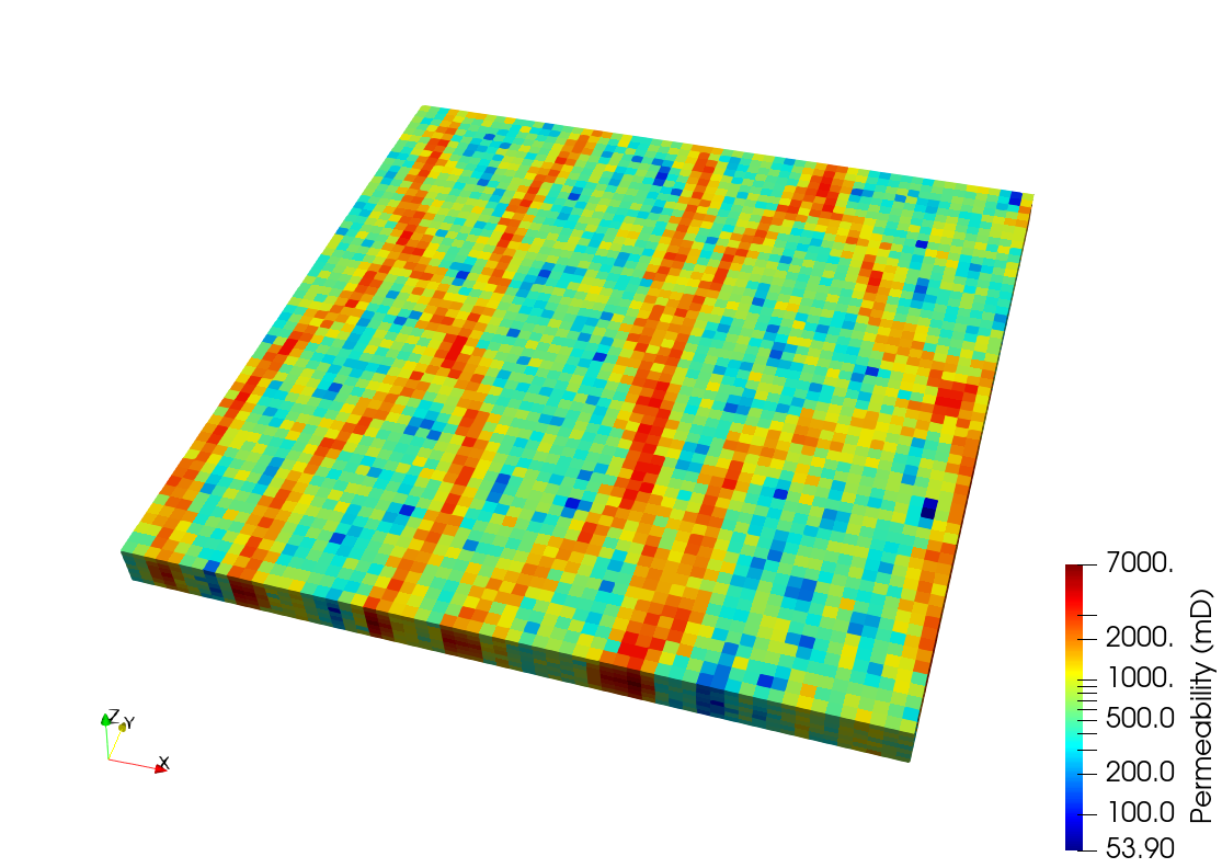
(a)

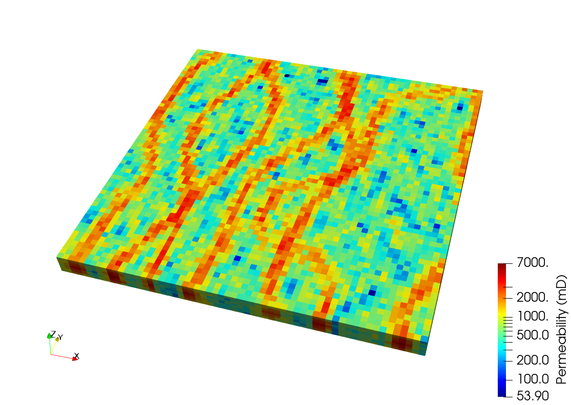
(b)

Figure 8: Two of the prior realisations for the EGG reservoir model.

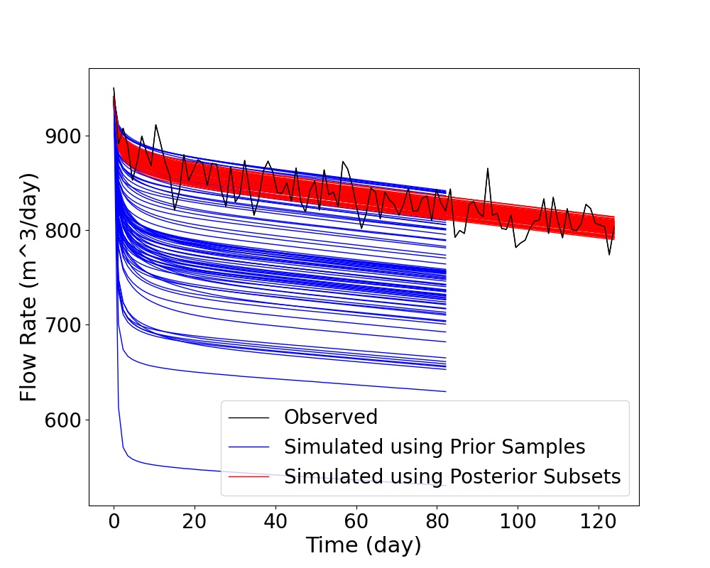
(a)

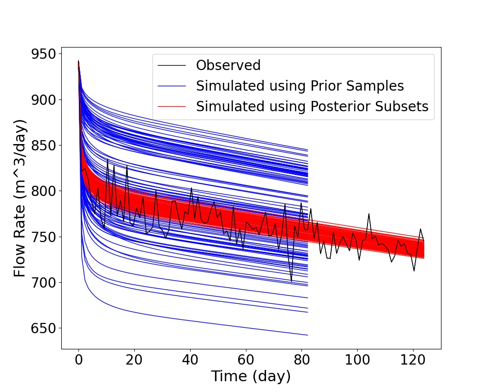
(b)

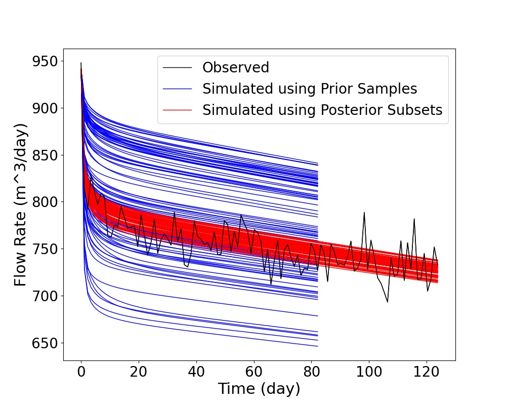
(c)

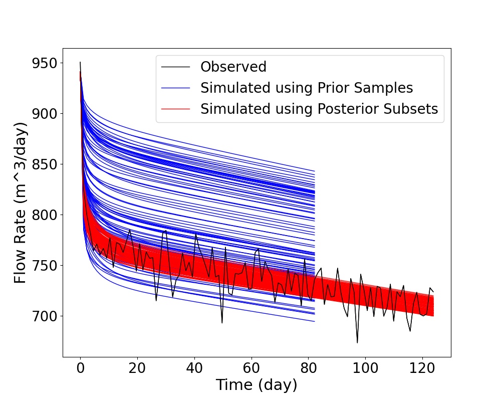
(d)

Figure 9: The simulated flow rates at wells using prior samples and posterior subsets by NEI (three samples in each subset) for the 3D non-Gaussian nonlinear inverse problem of transient Darcy flow in channelized reservoirs.

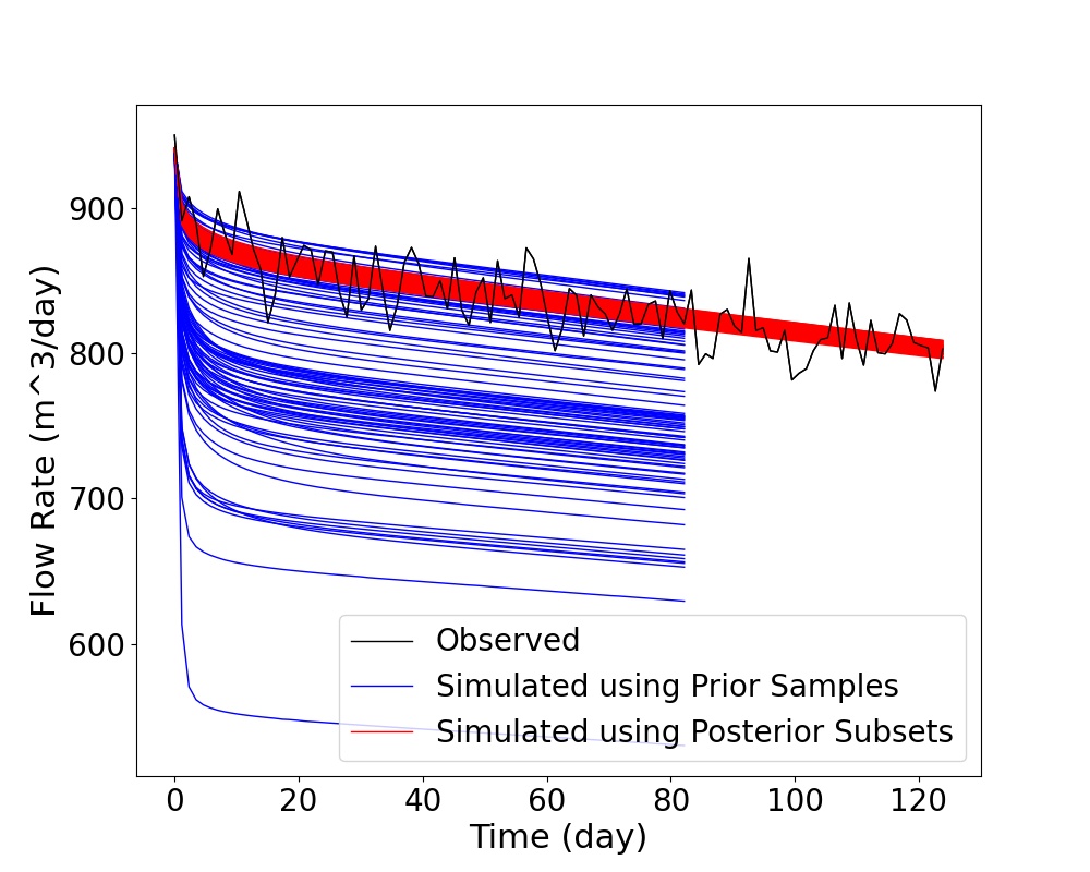
(a)

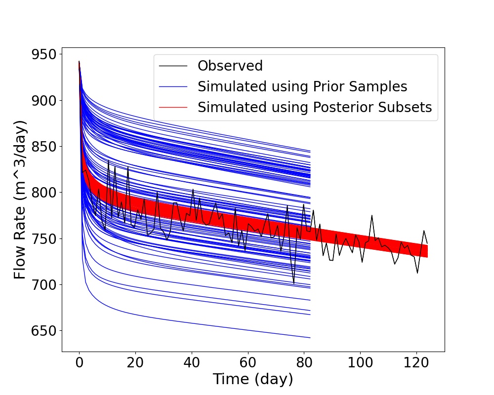
(b)

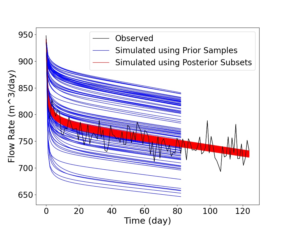
(c)

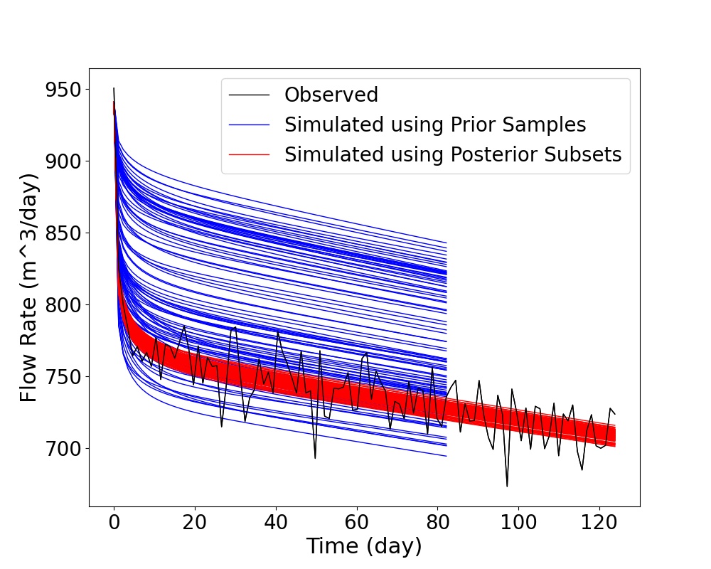
(d)

Figure 10: The simulated flow rates at wells using prior samples and posterior subsets by NEI (four samples in each subset) for the 3D non-Gaussian nonlinear inverse problem of transient Darcy flow in channelized reservoirs.

5 Conclusions

In the current study, a new inference method NEI is established based on the nonlinear expectation theory for direct uncertainty quantification of nonlinear inverse problems. Here, ’direct’ means that no repetitive runs of the forward model is needed in the inference process. Forward model runs are conducted only on the prior samples (realisations), followed by evaluations of linear expectations to yield the sublinear expectation for uncertainty quantification. Given noisy observed data and the likelihood function, the likelihood of each linear expectation is evaluated. The posterior linear expectations are those with highest likelihoods guided by the MLE principle. Then the posterior uncertainty is determined by the sublinear expectation based on the posterior linear expectations. For prediction, the non-repetitive samples in the posterior subsets are identified and simulated for a further period and the uncertainty of prediction is quantified using the corresponding sublinear expectation. The convergence of NEI is proved, and test cases of inferring uncertain parameters of transient Darcy flow are presented for validating the efficiency and accuracy of NEI.

Code Availability

The NEI codes are available at ”https://github.com/zhaozhang2022/nonlinearExp”. The prior samples can be generated using SGeMS or downloaded according to Jansen et al. (2014). The dynamic responses for prior samples can be obtained using a numerical simulator for solving the governing PDE.

References

- Arnold et al. (2019) Arnold, D., Demyanov, V., Rojas, T., Christie, M., 2019. Uncertainty quantification in reservoir prediction: Part 1—model realism in history matching using geological prior definitions. Mathematical Geosciences 51, 209–240.
- Caers (2011) Caers, J., 2011. Modeling uncertainty in the earth sciences. John Wiley & Sons.
- Chen et al. (2006) Chen, Z., Huan, G., Ma, Y., 2006. Computational methods for multiphase flows in porous media. SIAM.
- Choquet (1954) Choquet, G., 1954. Theory of capacities, in: Annales de l’institut Fourier, pp. 131–295.
- Cotter et al. (2013) Cotter, S.L., Roberts, G.O., Stuart, A.M., White, D., 2013. Mcmc methods for functions: modifying old algorithms to make them faster .
- Emerick and Reynolds (2013) Emerick, A.A., Reynolds, A.C., 2013. Ensemble smoother with multiple data assimilation. Computers & Geosciences 55, 3–15.
- Guo and Li (2021) Guo, X., Li, X., 2021. On the laws of large numbers for pseudo-independent random variables under sublinear expectation. Statistics & Probability Letters 172, 109042.
- Jansen et al. (2014) Jansen, J.D., Fonseca, R.M., Kahrobaei, S., Siraj, M., Van Essen, G., Van den Hof, P., 2014. The egg model–a geological ensemble for reservoir simulation. Geoscience Data Journal 1, 192–195.
- Ji et al. (2023) Ji, X., Peng, S., Yang, S., 2023. Imbalanced binary classification under distribution uncertainty. Information Sciences 621, 156–171.
- Jin and Peng (2021) Jin, H., Peng, S., 2021. Optimal unbiased estimation for maximal distribution. Probability, Uncertainty and Quantitative Risk 6, 189–198.
- Kaipio and Somersalo (2006) Kaipio, J., Somersalo, E., 2006. Statistical and computational inverse problems. volume 160. Springer Science & Business Media.
- Ma et al. (2020) Ma, X., Zhang, K., Yao, C., Zhang, L., Wang, J., Yang, Y., Yao, J., 2020. Multiscale-network structure inversion of fractured media based on a hierarchical-parameterization and data-driven evolutionary-optimization method. SPE Journal 25, 2729–2748.
- Olalotiti-Lawal and Datta-Gupta (2018) Olalotiti-Lawal, F., Datta-Gupta, A., 2018. A multiobjective markov chain monte carlo approach for history matching and uncertainty quantification. Journal of Petroleum Science and Engineering 166, 759–777.
- Oliver et al. (2008) Oliver, D.S., Reynolds, A.C., Liu, N., 2008. Inverse theory for petroleum reservoir characterization and history matching.
- Peaceman (1978) Peaceman, D.W., 1978. Interpretation of well-block pressures in numerical reservoir simulation. SPE Journal 18, 183–194.
- Peng (1997) Peng, S., 1997. Backward sde and related g-expectation. Pitman research notes in mathematics series , 141–160.
- Peng (2004) Peng, S., 2004. Filtration consistent nonlinear expectations and evaluations of contingent claims. Acta Mathematicae Applicatae Sinica, English Series 20, 191–214.
- Peng (2017) Peng, S., 2017. Theory, methods and meaning of nonlinear expectation theory. Scientia Sinica Mathematica 47, 1223–1254.
- Peng (2019) Peng, S., 2019. Nonlinear Expectations and Stochastic Calculus under Uncertainty: with Robust CLT and G-Brownian Motion. volume 95. Springer Nature.
- Peng et al. (2023) Peng, S., Yang, S., Yao, J., 2023. Improving value-at-risk prediction under model uncertainty. Journal of Financial Econometrics 21, 228–259.
- Pinski et al. (2015) Pinski, F.J., Simpson, G., Stuart, A.M., Weber, H., 2015. Algorithms for kullback–leibler approximation of probability measures in infinite dimensions. SIAM Journal on Scientific Computing 37, A2733–A2757.
- Posselt (2013) Posselt, D.J., 2013. Markov chain monte carlo methods: Theory and applications, in: Data Assimilation for Atmospheric, Oceanic and Hydrologic Applications (Vol. II). Springer, pp. 59–87.
- Povala et al. (2022) Povala, J., Kazlauskaite, I., Febrianto, E., Cirak, F., Girolami, M., 2022. Variational bayesian approximation of inverse problems using sparse precision matrices. Computer Methods in Applied Mechanics and Engineering 393, 114712.
- Remy et al. (2009) Remy, N., Boucher, A., Wu, J., 2009. Applied geostatistics with SGeMS: a user’s guide. Cambridge University Press.
- Smith (2013) Smith, R.C., 2013. Uncertainty quantification: theory, implementation, and applications. volume 12. Siam.
- Song et al. (2021) Song, X., Zheng, G.H., Jiang, L., 2021. Variational bayesian inversion for the reaction coefficient in space-time nonlocal diffusion equations. Advances in Computational Mathematics 47, 1–28.
- Stuart (2010) Stuart, A.M., 2010. Inverse problems: a bayesian perspective. Acta numerica 19, 451–559.
- Xiu (2010) Xiu, D., 2010. Numerical methods for stochastic computations: a spectral method approach. Princeton university press.
- Yan and Guo (2015) Yan, L., Guo, L., 2015. Stochastic collocation algorithms using l_1-minimization for bayesian solution of inverse problems. SIAM Journal on Scientific Computing 37, A1410–A1435.
- Yan and Zhou (2021) Yan, L., Zhou, T., 2021. Stein variational gradient descent with local approximations. Computer Methods in Applied Mechanics and Engineering 386, 114087.
- Zhang et al. (2021) Zhang, K., Zhang, J., Ma, X., Yao, C., Zhang, L., Yang, Y., Wang, J., Yao, J., Zhao, H., 2021. History matching of naturally fractured reservoirs using a deep sparse autoencoder. SPE Journal 26, 1700–1721.
- Zhang (2022) Zhang, Z., 2022. A physics-informed deep convolutional neural network for simulating and predicting transient darcy flows in heterogeneous reservoirs without labeled data. Journal of Petroleum Science and Engineering 211, 110179.
- Zhang et al. (2023) Zhang, Z., Yan, X., Liu, P., Zhang, K., Han, R., Wang, S., 2023. A physics-informed convolutional neural network for the simulation and prediction of two-phase darcy flows in heterogeneous porous media. Journal of Computational Physics 477, 111919.