Global convergence of block proximal iteratively reweighted algorithm with extrapolation

Abstract

In this paper, we propose a proximal iteratively reweighted algorithm with extrapolation based on block coordinate update aimed at solving a class of optimization problems which is the sum of a smooth possibly nonconvex loss function and a general nonconvex regularizer with a special structure. The proposed algorithm can be used to solve the $\ell_{p}(0<p<1)$ regularization problem by employing a updating strategy of the smoothing parameter. It is proved that there exists the nonzero extrapolation parameter such that the objective function is nonincreasing. Moreover, the global convergence and local convergence rate are obtained by using the Kurdyka-Łojasiewicz (KL) property on the objective function. Numerical experiments are given to indicate the efficiency of the proposed algorithm.

Key words. Iteraively reweighted algorithm; Kurdyka-Łojasiewicz property;
Block coordinate update; Extrapolation; Convergence analysis

1 Introduction

We mainly concentrate on the following optimization problem in this paper

$$\mathop{\min}_{{x}\in\mathbb{R}^{n}}\quad F({{x_{s_{1}}}},{{x_{s_{2}}}},\dots,{{x_{s_{m}}}}):=f({{x_{s_{1}}}},{{x_{s_{2}}}},\dots,{{x_{s_{m}}}})+\lambda\sum_{i=1}^{m}\sum_{j\in{{{s_{i}}}}}h(g({{x_{j}}})),\,\lambda>0,$$ (1)

where $f,g$ and $h$ are of the below properties.

Assumption 1.

1. $f:\mathbb{R}^{n}\rightarrow\mathbb{R}$ is a continuously differentiable function and has a block Lipschitz continuous gradient constant, i.e., for some disjoint sets $\{{{x_{s_{1}}}},{{x_{s_{2}}}},\dots,{{x_{s_{m}}}}\}$ satisfying $\cup{\{{s_{1}},{{{s_{1}}}},\dots,{s_{m}}}\}=\{1,2,\dots,n\}$, it has that

   $$\|\nabla_{{s_{j}}}f({{x_{s_{1}}}},\dots,{{x_{s_{j}}}},\dots,{{x_{s_{m}}}})-\nabla_{{s_{j}}}f({{x_{s_{1}}}},\dots,{{\hat{x}_{s_{j}}}},\dots,{{x_{s_{m}}}})\|\leq L_{j}\|{x_{s_{j}}}-{\hat{x}_{s_{j}}}\|,$$ (2)

   and there exist constants $0<\ell\leq L<\infty$ satisfying $\ell\leq L_{j}\leq L$ for any $j\in\{{{{s_{1}}}},{{{s_{2}}}},\dots,{{{s_{m}}}}\};$

2. $g:\mathbb{R}\to\mathbb{R}$ is a nonnegative closed and convex function ;

3. $h:\rm{Im(g)}\to\mathbb{R}_{+}$ is a concave function and satisfies  $h^{\prime}(t)>0$,  $\forall\,t\in{\rm{Im}}(g)$. Moreover, it is differentiable with a Lipschitz continuous gradient $L_{h}$, i.e., for any $s,t\in{\rm{Im}}(g)$,

   $$|h^{\prime}(s)-h^{\prime}(t)|\leq L_{h}|s-t|;$$

4. $F$ is coercive, that is when $\|x\|\to+\infty$, $F\to+\infty$.

The model (1) has wide applications which arise in compressive sensing [11], variable selections [8] and signal processing [9] and so on. The former item of the model (1) is generally a loss function which is smooth and may be nonconvex, such as $f(x)=\frac{1}{n}\sum_{i=1}^{n}{\rm{log}}(1+{\rm{exp}}(-b_{i}a^{T}_{i}x))$, where $A=[a^{T}_{1};\dots;a^{T}_{n}]\in\mathbb{R}^{n\times d},b\in\mathbb{R}^{n}$. The later item of the model (1) can be can be viewed as a regularization or penalty component, such as the log penalty function [7], the approximate $\ell_{p}$ norm [8] and so on. When $s_{j}=\{j\},$ the problem (1) reduces to the following univariate problem,

$$\mathop{\min}_{x\in\mathbb{R}^{n}}\quad F(x):=f(x)+\lambda\sum_{i=1}^{n}h(g(x_{i}),\,\lambda>0.$$ (3)

Lu et al.[15] have developed the proximal iteratively reweighted algorithm (PIRE) for solving the problem (3),

$$x^{k+1}=\arg\min_{x}\sum^{n}_{i=1}w^{k}_{i}g(x_{i})+\frac{L}{2}\|x-(x^{k}-\frac{1}{L}\nabla f(x^{k}))\|^{2},$$ (4)

where $w^{k}_{i}:=\lambda h^{\prime}(g(x^{k}_{i}))$ and $L>0$. It needs to be mentioned that the subproblem (4) has a unique solution since the subproblem (4) is strongly convex. Additionally, the solution has an explicit form when the proximal operator of $g$ is easily calculated. Only subsequence convergence of the PIRE algorithm is obtained in [15]. To deeply discuss the convergence of the PIRE algorithm, Sun et al. [22] strengthened the condition on the objective, i.e., it is required that $h$ is continuously differentiable and has a Lipschitz continuous gradient on the image set of function $g$ and proved the global convergence of the algorithmic sequence under the Kurdyka-Łojasiewicz(KL) property on the objective function $F$. Their algorithmic framework unifies the PIRE, the Proximal Iteratively Reweighted algorithm with parallel splitting (PIRE-PS) and the Proximal Iteratively Reweighted algorithm with alternative updating (PIRE-AU).

It is well known that extrapolation technique proposed by Nesterov [21] has been an effective way to improve the first order algorithms. Recently, Yu and Pong [28] proposed the iteratively reweighted $\ell_{1}$ algorithm with three different extrapolation ways based on Nesterov’s method and its extentions [4, 3, 23, 14, 10, 12] to solve the following problem,

$$\min_{x\in\mathbb{R}^{n}}F(x):=f(x)+\delta_{C}(x)+\sum_{i=1}^{n}\phi(|y_{i}|),$$ (5)

where $f:\mathbb{R}^{n}\to\mathbb{R}$ is a smooth convex function with a Lipschitz continuous gradient, $C$ is a nonempty closed convex set, $\phi:\mathbb{R}_{+}\to\mathbb{R}_{+}$ is a continuous concave function and continuously differentiable on $(0,+\infty)$ and satisfies $\phi(0)=0$. Moreover, it is assumed that $\lim_{t\to 0}\phi^{\prime}(t)$ exists. It is observed that the model (1) and(5) are not the same. The global convergence is obtained under KL property on certain potential functions.

Benefitted from the advantages of the extrapolation technique, Xu and Yin [26] proposed a block proximal gradient method with extrapolation based on the fixed cyclic order of each block to solve the optimization problem that the feasible set and objective function are convex in each block of variables. The global convergence of the algorithmic sequence is obtained under the KL condition. Further, Xu and Yin [27] considered the problem which is the sum of two nonconvex functions and always require the proximal operator of the nonsmooth component is easily calculated. They developed a proximal gradient method with the extrapolation term based on block update and each block is updated at least once either deterministically cyclic or randomly shuffled for each cycle. They proved that there exists a nonzero extrapolation parameter such that the objective function is nonincreasing under certain conditions and get the same convergence under the KL property.

Witnessing the success of accelerated methods mentioned above, in this paper, we propose a iteratively reweighted algorithm with extrapolation based on the block coordinate update to solve problem (1), in which the proximal operator of the regularization may not have a closed form solution. Each block is updated at least once within fixed iterations, either through deterministic cycling or through random shuffles. Especially, the proposed algorithm could be used to solve the $\ell_{p}(0<p<1)$ regularization problem by using a existing update strategy of smoothing factor. We get that the existence of nonzero extrapolation parameters makes the objective function nonincreasing. Further, by imposing the assumption of KL property on the objective function, we prove that the global convergence and local convergence rate of the sequence generated by the BPIREe algorithm.

The composition of the paper includes the following parts. Some preparatory work is given in Section 2. and in Section 3, we propose a BPIREe algorithm and analyze its convergence behaviour. Further, in Section 4 we apply the proposed algorithm to solve the $\ell_{p}$ reguralization problem and discuss its convergence. Section 4 illustrates the performance of the proposed algorithm through numerical experiments. At last, we give the conclusions in Section 5.

Notations. The sets $\mathbb{R}^{n}$, $\mathbb{R}^{n}_{+}$ and $\mathbb{R}^{n}_{++}$ represent $n$-dimensional Euclidean space, positive orthant in $\mathbb{R}^{n}$ and the interior of $\mathbb{R}^{n}$ respectively. For $x\in\mathbb{R}^{n}$, $\|x\|:=\|x\|_{2}=(\sum_{i=1}^{n}x^{2}_{i})^{\frac{1}{2}}$ denotes the Euclidean norm. $\|x\|_{p}=(\sum_{i=1}^{n}|x_{i}|^{p})^{\frac{1}{p}}(0<p<1)$ represents the $\ell_{p}$ norm. The Hadamard product for any two vectors $a,b\in\mathbb{R}^{n}$ is defined as $(a\odot b)_{i}=a_{i}b_{i}$. Denote $\mathbb{N}=\{0,1,\dots,n\}$. Let $\{-1,0,1\}^{n}$ be the set of $n$-dimensional vectors with components drawn from $\{-1,0,1\}$. $\rm{Im}(g)$ represents the image set of function $g$. The set $\mathbb{R}^{m\times n}$ is denoted as the space of $m\times n$ matrices. For any $A=[a_{i,j}]_{m\times n}\in\mathbb{R}^{m\times n}$, the Frobenius norm of $X$ is defined ad $\|A\|_{F}=\sqrt{\sum_{i,j}a^{2}_{i,j}}$. Denote $A^{T}$ be the transpose of the matrix $A$.

2 Preliminaries

In this section, we mainly recall some definitions and preliminary results which will be helpful for the analysis of this paper.

The domain of an extended real-valued function $\phi:\mathbb{R}^{n}\to(-\infty,+\infty]$ is defined as ${\rm{dom}}\,\phi:=\{x\in\mathbb{R}^{n},\phi(x)<+\infty\}$. If the domain is nonempty, it is said to be proper. The function $\phi$ is said to be closed if it is lower semicontinuous.

Definition 2.1.

(subdifferential [17, 20]) Let $\phi(x):\mathbb{R}^{n}\to({-\infty},{+\infty}]$ be a proper and closed function. The limiting-subdifferential (or subdifferential) is the set of all vectors $u\in\mathbb{R}^{n}$ satisfying

$$\partial\phi(x):=\left\{u\in\mathbb{R}^{n}|\exists x^{k}\to x,\,\phi(x^{k})\to\phi(x)\,{\rm{and}}\,u^{k}\in\hat{\partial}\phi(x^{k}),\,u^{k}\to u\,{\rm{as}}\,k\to+\infty\right\},$$

where $\hat{\partial}\phi(x)$ is the Fréchet subdifferential of $\phi$ at $x$, if $x\in{\rm{dom}}\phi$, defined by

$$\lim_{y\neq x}\inf_{y\to x}\frac{\phi(y)-\phi(x)-\langle u,y-x\rangle}{\|x-y\|}\geq 0,$$

otherwise, we set $\hat{\partial}\phi(x)=\emptyset$.

If $\phi$ is continuously differentiable, then $\partial\phi=\{\nabla\phi\}$. When $\phi$ is convex, the subdifferential reduces to the classical subdifferential in the sense of convex analysis

$$\partial\phi(x):=\{u:\phi(y)-\phi(x)\geq\langle u,y-x\rangle\}.$$

The Kurdyka-Łojasiewicz property [6, 2] is useful for the convergence analysis of first order methods, which apply to a wide range of problems, including nonsmooth semialgebraic minimization problems [2, 1].

Definition 2.2.

(Kurdyka-Łojasiewicz property) Let $J(x):\mathbb{R}^{n}\to({-\infty},{+\infty}]$ be a proper closed function, the function $J(x)$ is said to have the Kurdyka- Łojasiewicz (KL) property at $\bar{x}\in{\rm{dom}}\partial J:=\left\{x\in\mathbb{R}^{n}:\partial J(x)\neq\emptyset\right\}$ if there exists a neighborhood $U$ of $\bar{x}$, $\xi\in(0,+\infty]$, and a function $\phi:[0,\xi)\to\mathbb{R}_{+}$ satisfying

1. $\phi(0)=0,\phi\in C^{1}(0,\xi)$;

2. for all $s\in(0,\xi),{\phi}^{\prime}(s)>0$;

3. for any $x\in U\cap[J(\bar{x})<J(x)<J({\bar{x}})+\xi]$,

it holds that

$$\phi{{}^{\prime}}(J(x)-J(\bar{x}))\cdot{\rm{dist}}(0,\partial J(x))\geq 1.$$ (6)

If $J$ satisfies the KL property at each point of ${\rm{dom}}J$, then $J$ is called a KL function. If $J$ satisfies the KL property at $\bar{x}$ and $\phi$ in (6) is chosen as $\phi(s)=cs^{1-\theta}$ for some $\theta\in[0,1)$, $c>0$, then we can say that $J$ satisfies the KL property at $\bar{x}$ with exponent $\alpha$.

If $f$ is smooth, then the inequality (6) reduces to the following given by Attouch et al. [1]

$$\|\nabla(\phi\circ J)\|\geq 1.$$

Lemma 2.3.

([20]) Under the Assumption 1(ii), there exists a $L_{g}>0$ such that

$$|g(x)-g(y)|\leq L_{g}|x-y|,$$

for any $x,y\in S$ where $S$ is a bounded closed set.

3 Block Proximal Iteratively Reweightly Algorithm with Extrapolation

Inspired by the extrapolation technique  [21] and block update mode in [27], we propose a block proximal iteratively reweighted algorithm which only requires that each block can be updated at least once within the fixed number of iterations. For a selected update block $b_{k}\in\{s_{1},\dots,s_{m}\}$ in iteration $k$, the specific form is as follows

$$\begin{cases}{x}^{k}_{s_{i}}={x}^{k-1}_{s_{i}},&\text{ if }s_{i}\neq b_{k};\\ {x}^{k}_{s_{i}}=\arg\min_{{x}_{s_{i}}}\{\langle\nabla_{{s_{i}}}f({x}^{k-1}_{\neq{s_{i}}},{\hat{x}}^{k}_{s_{i}}),{x}_{s_{i}}\rangle+\frac{1}{2\alpha_{k}}\|{x}_{s_{i}}-{\hat{x}}^{k}_{s_{i}}\|^{2}+\sum_{j\in s_{i}}w^{k-1}_{j}g({x}_{j})\},&\text{ if }s_{i}=b_{k},\\ \end{cases}$$ (7)

where $\alpha_{k}$ is the stepsize, $({x}^{k-1}_{\neq{s_{i}}},{\hat{x}}^{k}_{s_{i}})$ represents the point $({x}^{k-1}_{1},\dots,{x}^{k-1}_{s_{i}-1},{\hat{x}}^{k}_{s_{i}},{x}^{k-1}_{s_{i}+1},\dots,{x}^{k-1}_{s_{m}})$, $w^{k-1}_{j}=\lambda h^{\prime}(g({x}^{k-1}_{j}))$ and the extrapolation item is

$${\hat{x}}^{k}_{s_{i}}={x}^{k-1}_{s_{i}}+\beta_{k}({x}^{k-1}_{s_{i}}-{x}^{\rm{prev}}_{s_{i}}),$$

where $\beta_{k}$ is the extrapolation parameter and ${x}^{\rm{prev}}_{s_{i}}$ is the last updated value of ${x}^{k-1}_{s_{i}}$.

Algorithm 1 BPIREe algorithm

1:  Initialization: $x^{-1}=x^{0}$.

2:  for all $k=1,2,\dots$ do

3:     Choose $b_{k}\in\{s_{1},s_{2},\dots,s_{m}\}$ in a deterministic or random manner.

4:     ${x}^{k}\leftarrow(\ref{2.3})$ where $\alpha_{k},\beta_{k}$ satisfying certain conditions.

5:     if stopping criterion is satisfied then

6:        return ${x}^{k}$.

7:     end if

8:  end for

The following extra notations are required in this paper since the update can not be periodic. When the algorithm is updated to the $k$th iteration, we use $\mathcal{K}[s_{i},k]$ to represent the set of iterations of the block $s_{i}$, that is,

$$\mathcal{K}[s_{i},k]:=\{\kappa:b_{\kappa}=s_{i},1\leq\kappa\leq k\}\subseteq\{1,\dots,k\},$$

and $d^{k}_{s_{i}}:=|\mathcal{K}[s_{i},k]|$ to signify the number of the updated iterations for $s_{i}$th block. Then $\cup_{i=1}^{m}\mathcal{K}[s_{i},k]=[k]:=\{1,2,\dots,k\}$ and $\sum_{i=1}^{m}d^{k}_{s_{i}}=k$.

After $k$th iteration, denote ${x}^{k}$ be the value of ${x}$; and after $j$th update, ${\tilde{x}}^{j}_{s_{i}}$ means the value of ${\tilde{x}}_{s_{i}}$ for block $s_{i}$. Letting $j=d^{k}_{s_{i}}$, then ${x}^{k}_{s_{i}}={\tilde{x}}^{j}_{s_{i}}$. For $s_{i}=b_{k}$, $j=d^{k}_{s_{i}}$, the extrapolated point can be indicated as

$${\hat{x}}^{k}_{s_{i}}={\tilde{x}}^{j-1}_{s_{i}}+\beta_{k}({\tilde{x}}^{j-1}_{s_{i}}-{\tilde{x}}^{j-2}_{s_{i}}),\quad 0\leq\beta_{k}\leq 1.$$ (8)

The extrapolation coefficient and Lipschitz constant are divided into $m$ disjoint subsets, which are denoted as

$$\{\beta_{\kappa}:1\leq\kappa\leq k\}=\cup_{i=1}^{m}\{\beta_{\kappa}:\kappa\in\mathcal{K}[s_{i},k]\}:=\cup_{i=1}^{m}\{\tilde{\beta}^{j}_{s_{i}}:1\leq j\leq d^{k}_{s_{i}}\},$$ (9)

$$\{L_{\kappa}:1\leq\kappa\leq k\}=\cup_{i=1}^{m}\{L_{\kappa}:\kappa\in\mathcal{K}[s_{i},k]\}:=\cup_{i=1}^{m}\{\tilde{L}^{j}_{s_{i}}:1\leq j\leq d^{k}_{s_{i}}\}.$$ (10)

For a certain block $s_{i}$, the specific forms of the sequence ${x_{s_{i}}}$, Lipschitz constant and the extrapolation parameter are denoted as follows

$$\,{\tilde{x}}^{1}_{s_{i}},{\tilde{x}}^{2}_{s_{i}},\dots,{\tilde{x}}^{d^{k}_{s_{i}}}_{s_{i}}\dots;$$ (11)

$$\,\tilde{L}^{1}_{s_{s_{i}}},\tilde{L}^{2}_{s_{i}},\dots,\tilde{L}^{d^{k}_{s_{i}}}_{s_{i}},\dots;$$ (12)

$$\,\tilde{\beta}^{1}_{s_{i}},\tilde{\beta}^{2}_{s_{i}},\dots,\tilde{\beta}^{d^{k}_{s_{i}}}_{s_{i}}.\dots.$$ (13)

The stepsize and extrapolation parameter are set as follows

$$\alpha_{k}=\frac{1}{2L_{k}},\quad\tilde{\beta}^{j}_{s_{i}}\leq\frac{\delta}{6}\sqrt{\frac{\tilde{L}^{j-1}_{s_{i}}}{\tilde{L}^{j}_{s_{i}}}},\,\,\,\delta<1.$$ (14)

We make the following assumptions, which will be used in the convergence analysis.

Assumption 2.

(Essentially cyclic block update). In Algorithm 1, every block is updated at least once within any $T(T\geq m)$ consecutive iterations.

Lemma 3.1.

Suppose $\{x^{k}\}$ is a sequence generated by BPIREe algorithm, ${\alpha_{k}}$ and $\beta_{k}$ are chosen as in (14), under the Assumption 1, it has that

$$F(x^{k-1})-F(x^{k}) \geq c_{1}\tilde{L}^{j}_{s_{i}}\|\tilde{x}^{j-1}_{s_{i}}-\tilde{x}^{j}_{s_{i}}\|^{2}-c_{2}\tilde{L}^{j}_{s_{i}}(\tilde{\beta}^{j}_{s_{i}})^{2}\|\tilde{x}^{j-2}_{s_{i}}-\tilde{x}^{j-1}_{s_{i}}\|^{2}$$ (15)

$$\geq c_{1}\tilde{L}^{j}_{s_{i}}\|\tilde{x}^{j-1}_{s_{i}}-\tilde{x}^{j}_{s_{i}}\|^{2}-\frac{c_{2}\tilde{L}^{j-1}_{s_{i}}}{36}\delta^{2}\|\tilde{x}^{j-2}_{s_{i}}-\tilde{x}^{j-1}_{s_{i}}\|^{2},$$ (16)

where $c_{1}=\frac{1}{4}$, $c_{2}=9$, $s_{i}=b_{k}$ and $j=d^{k}_{s_{i}}$.

Proof.

Since $f$ is gradient Lipschitz continuous concerning each block $s_{i}$ from Assumption 1(i), it yields that

$$f(x^{k})\leq f(x^{k-1})+\langle\nabla_{{s_{i}}}f(x^{k-1}),x^{k}_{s_{i}}-x^{k-1}_{s_{i}}\rangle+\frac{L_{k}}{2}\|x^{k}_{s_{i}}-x^{k-1}_{s_{i}}\|^{2}.$$ (17)

From the optimality of subproblem (7), we have

$$\langle\nabla_{{s_{i}}}f(x^{k-1}_{\neq{s_{i}}},\hat{x}^{k}_{s_{i}}),x^{k}_{s_{i}}\rangle+\frac{1}{2\alpha_{k}}\|x^{k}_{s_{i}}-\hat{x}^{k}_{s_{i}}\|^{2}+\sum_{j\in s_{i}}w^{k-1}_{j}g(x^{k}_{j})$$

$$\leq \langle\nabla_{{s_{i}}}f(x^{k-1}_{\neq{s_{i}}},\hat{x}^{k}_{s_{i}}),x^{k-1}_{s_{i}}\rangle+\frac{1}{2\alpha_{k}}\|x^{k-1}_{s_{i}}-\hat{x}^{k}_{s_{i}}\|^{2}+\sum_{j\in s_{i}}w^{k-1}_{j}g(x^{k-1}_{j}),$$ (18)

Notice $x^{k-1}_{s_{j}}=x^{k}_{s_{j}},\forall j\neq i$. It then follows that

$$F(x^{k-1})-F(x^{k})$$

$$= f(x^{k-1})+\sum_{j\in s_{i}}h(g(x^{k-1}_{j}))-f(x^{k})-\sum_{j\in s_{i}}h(g(x^{k}_{j}))$$

$$\geq \langle\nabla_{{s_{i}}}f(x^{k-1}),x^{k-1}_{s_{i}}-x^{k}_{s_{i}}\rangle-\frac{L_{k}}{2}\|x^{k}_{s_{i}}-x^{k-1}_{s_{i}}\|^{2}+\sum_{j\in s_{i}}h^{\prime}(g(x^{k-1}_{j}))(g(x^{k-1}_{j})-g(x^{k}_{j}))$$

$$\geq \langle\nabla_{{s_{i}}}f(x^{k-1}),x^{k-1}_{s_{i}}-x^{k}_{s_{i}}\rangle-\frac{L_{k}}{2}\|x^{k}_{s_{i}}-x^{k-1}_{s_{i}}\|^{2}+\langle\nabla_{{s_{i}}}f(x^{k-1}_{\neq{s_{i}}},\hat{x}^{k}_{s_{i}}),x^{k}_{s_{i}}-x^{k-1}_{s_{i}}\rangle$$

$$+\frac{1}{2\alpha_{k}}\|x^{k}_{s_{i}}-\hat{x}^{k}_{s_{i}}\|^{2}-\frac{1}{2\alpha_{k}}\|x^{k-1}_{s_{i}}-\hat{x}^{k}_{s_{i}}\|^{2}$$

$$= \langle\nabla_{{s_{i}}}f(x^{k-1})-\nabla_{{s_{i}}}f(x^{k-1}_{\neq{s_{i}}},\hat{x}^{k}_{s_{i}}),x^{k-1}_{s_{i}}-x^{k}_{s_{i}}\rangle+\frac{1}{\alpha_{k}}\langle x^{k}_{s_{i}}-x^{k-1}_{s_{i}},x^{k-1}_{s_{i}}-\hat{x}^{k}_{s_{i}}\rangle$$

$$+(\frac{1}{2\alpha_{k}}-\frac{L_{k}}{2})\|x^{k}_{s_{i}}-x^{k-1}_{s_{i}}\|^{2}$$

$$\geq -\|x^{k-1}_{s_{i}}-x^{k}_{s_{i}}\|(\|\nabla_{{s_{i}}}f(x^{k-1})-\nabla_{{s_{i}}}f(x^{k-1}_{\neq{s_{i}}},\hat{x}^{k}_{s_{i}})\|+\frac{1}{\alpha_{k}}\|x^{k-1}_{s_{i}}-\hat{x}^{k}_{s_{i}}\|)+(\frac{1}{2\alpha_{k}}-\frac{L_{k}}{2})\|x^{k}_{s_{i}}-x^{k-1}_{s_{i}}\|^{2}$$

$$\geq -(\frac{1}{\alpha_{k}}+L_{k})\|x^{k-1}_{s_{i}}-x^{k}_{s_{i}}\|\cdot\|x^{k-1}_{s_{i}}-\hat{x}^{k}_{s_{i}}\|+(\frac{1}{2\alpha_{k}}-\frac{L_{k}}{2})\|x^{k}_{s_{i}}-x^{k-1}_{s_{i}}\|^{2}$$

$$= -(\frac{1}{\alpha_{k}}+L_{k})\beta_{k}\|x^{k-1}_{s_{i}}-x^{k}_{s_{i}}\|\cdot\|x^{k-1}_{s_{i}}-\tilde{x}^{d^{k-1}_{s_{i}}-1}_{s_{i}}\|+(\frac{1}{2\alpha_{k}}-\frac{L_{k}}{2})\|x^{k}_{s_{i}}-x^{k-1}_{s_{i}}\|^{2}$$

$$\geq \frac{1}{4}(\frac{1}{\alpha_{k}}-L_{k})\|x^{k-1}_{s_{i}}-x^{k}_{s_{i}}\|^{2}-\frac{(\frac{1}{\alpha_{k}}+L_{k})^{2}}{\frac{1}{\alpha_{k}}-L_{k}}\beta^{2}_{k}\|x^{k-1}_{s_{i}}-\tilde{x}^{d^{k-1}_{s_{i}}}_{s_{i}}\|^{2},$$

where the first inequality derives from (17) and the concavity of $h$, the second inequality from (3), the forth inequality derives from Cauchy-Schwarz inequality and the fifth inequality holds due to Young’s inequality $ab\leq\frac{1}{\frac{1}{\alpha_{k}}-L_{k}}a^{2}+(\frac{1}{\alpha_{k}}-L_{k})\frac{1}{4}b^{2}$ for any $a,b\geq 0$ with $a=(\frac{1}{\alpha_{k}}+L_{k})\beta_{k}\|x^{k-1}_{s_{i}}-\tilde{x}^{d^{k-1}_{s_{i}}-1}_{s_{i}}\|$ and $b=\|x^{k}_{s_{i}}-x^{k-1}_{s_{i}}\|$. Then the result is obtained by choosing $\alpha_{k}$ and $\beta_{k}$ defined as in (14). ∎

Remark 1.

When $\alpha_{k}=\frac{1}{\gamma L_{k}}$ and $\tilde{\beta}^{j}_{s_{i}}\leq\frac{\delta(\gamma-1)}{2(\gamma+1)}\sqrt{{\tilde{L}^{j-1}_{s_{i}}/\tilde{L}^{j}_{s_{i}}}}$, $\forall\gamma>1$ and some $\delta<1$. Then (16) holds with $c_{1}=\frac{\gamma-1}{4}$ and $c_{2}=\frac{(\gamma+1)^{2}}{\gamma-1}$. In a more general case, if $0<\inf_{k}\alpha_{k}\leq\sup_{k}\alpha_{k}<\infty$, then (16) holds with $c_{1}>0$, $c_{2}>0$ and $\tilde{\beta}^{j}_{s_{i}}\leq\delta\sqrt{c_{1}{\tilde{L}^{j-1}_{s_{i}}/c_{2}\tilde{L}^{j}_{s_{i}}}}$ for some $\delta<1$.

Remark 2.

Since $d^{k}_{s_{i}}=d^{k-1}_{s_{i}}+1$ for $s_{i}=b_{k}$ and $d^{k}_{s_{i}}=d^{k-1}_{s_{i}},\forall{s_{i}}\neq b_{k}$, $\sum_{i=p}^{q}a_{j}=0$ when $q<p$, the inequality (16) can be rewritten as

$$F(x^{k+1})-F(x^{k})\geq \sum_{i=1}^{m}\sum_{j=d^{k-1}_{s_{i}}}^{d^{k}_{s_{i}}}\frac{1}{4}(\tilde{L}^{j}_{s_{i}}\|\tilde{x}^{j-1}_{s_{i}}-\tilde{x}^{j}_{s_{i}}\|^{2}-\tilde{L}^{j-1}_{s_{i}}\delta^{2}\|\tilde{x}^{j-2}_{s_{i}}-\tilde{x}^{j-1}_{s_{i}}\|^{2}).$$ (19)

Corollary 3.2.

Suppose $\{x^{k}\}$ is a sequence generated by BPIREe algorithm, when $f$ is convex with respect to each block of variables and $\alpha_{k}=\frac{1}{L_{k}}$, under the Assumption 1, it holds that

$$F(x^{k-1})-F(x^{k})\geq-\frac{L_{k}\beta^{2}_{k}}{2}\|x^{k-1}_{s_{i}}-x^{d^{k-1}_{s_{i}}-1}_{s_{i}}\|^{2}+\frac{L_{k}}{2}\|x^{k}_{s_{i}}-x^{k-1}_{s_{i}}\|^{2}.$$

Proof.

From (17), we get

$$F(x^{k-1})-F(x^{k})$$

$$= f(x^{k-1})-f(x^{k})+\sum_{j\in s_{i}}h(g(x^{k-1}_{j}))-\sum_{j\in s_{i}}h(g(x^{k}_{j}))$$

$$\geq f(x^{k-1})-f(x^{k-1}_{\neq{s_{i}}},\hat{x}^{k}_{s_{i}})-\langle\nabla f(x^{k-1}_{\neq{s_{i}}},\hat{x}^{k}_{s_{i}}),x^{k}_{s_{i}}-\hat{x}^{k}_{s_{i}}\rangle-\frac{L_{k}}{2}\|x^{k}_{s_{i}}-\hat{x}^{k}_{s_{i}}\|^{2}$$

$$\,+\lambda\sum_{j\in s_{i}}h^{\prime}(g(x^{k-1}_{j}))(g(x^{k-1}_{j})-g(x^{k}_{j}))$$

$$\geq f(x^{k-1})-f(x^{k-1}_{\neq{s_{i}}},\hat{x}^{k}_{s_{i}})-\langle\nabla f(x^{k-1}_{\neq{s_{i}}},\hat{x}^{k}_{s_{i}}),x^{k}_{s_{i}}-\hat{x}^{k}_{s_{i}}\rangle-\frac{L_{k}}{2}\|x^{k}_{s_{i}}-\hat{x}^{k}_{s_{i}}\|^{2}$$

$$+\langle\nabla f(x^{k-1}_{\neq{s_{i}}},\hat{x}^{k}_{s_{i}}),x^{k}_{s_{i}}-x^{k-1}_{s_{i}}\rangle+\frac{L_{k}}{2}\|x^{k}_{s_{i}}-\hat{x}^{k}_{s_{i}}\|^{2}-\frac{L_{k}}{2}\|x^{k-1}_{s_{i}}-\hat{x}^{k}_{s_{i}}\|^{2}+\frac{L_{k}}{2}\|x^{k}_{s_{i}}-x^{k-1}_{s_{i}}\|^{2}$$

$$= f(x^{k-1})-f(x^{k-1}_{\neq{s_{i}}},\hat{x}^{k}_{s_{i}})-\langle\nabla f(x^{k-1}_{\neq{s_{i}}},\hat{x}^{k}_{s_{i}}),x^{k-1}_{s_{i}}-\hat{x}^{k}_{s_{i}}\rangle-\frac{L_{k}}{2}\|x^{k-1}_{s_{i}}-\hat{x}^{k}_{s_{i}}\|^{2}$$

$$\,+\frac{L_{k}}{2}\|x^{k}_{s_{i}}-x^{k-1}_{s_{i}}\|^{2}$$

$$\geq -\frac{L_{k}}{2}\|x^{k-1}_{s_{i}}-\hat{x}^{k}_{s_{i}}\|^{2}+\frac{L_{k}}{2}\|x^{k}_{s_{i}}-x^{k-1}_{s_{i}}\|^{2}$$

$$= -\frac{L_{k}\beta^{2}_{k}}{2}\|x^{k-1}_{s_{i}}-x^{d^{k-1}_{s_{i}}-1}_{s_{i}}\|^{2}+\frac{L_{k}}{2}\|x^{k}_{s_{i}}-x^{k-1}_{s_{i}}\|^{2},$$

where the first inequality derives from (17) and the concavity of $h$, the second inequality holds due to the strong convexity of the subproblem (7) and the third inequality comes from the convexity of $f$. This completes the proof. ∎

Remark 3.

It is observed that when $f$ is convex concerning each block of variables, the inequality (15) holds with $c_{1}=c_{2}=\frac{1}{2}$ and the extrapolation parameter can be chosen as $\beta^{2}_{k}\leq{(\tilde{L}^{j-1}_{s_{i}}\delta^{2})/\tilde{L}^{j}_{s_{i}}}\,(\delta<1)$.

Assumption 3.

For any $k\in\mathbb{N}$, the extrapolation parameter $\beta_{k}$ is chosen to satisfy $F(x^{k})\leq F(x^{k-1})$.

Now we make an illustration of the Assumption 3 is rational.

Lemma 3.3.

For any $s_{i}=b_{k}$, suppose

$$x^{k-1}_{s_{i}}\notin\arg\min_{{s_{i}}}\{\langle\nabla_{{s_{i}}}f(x^{k-1}),x_{s_{i}}-x^{k-1}_{s_{i}}\rangle+\frac{1}{2\alpha_{k}}\|x_{s_{i}}-x^{k-1}_{s_{i}}\|^{2}+\sum_{j\in s_{i}}w^{k-1}_{j}g(x_{j})\},$$ (20)

then there exists $\bar{\beta}_{k}>0$ such that $F(x^{k})\leq F(x^{k-1})$ for any $\beta_{k}\in[0,\bar{\beta}_{k}]$.

Proof.

Since the subproblem (20) is strongly convex, the proximal operator of $\alpha_{k}\sum_{j\in s_{i}}w^{k-1}_{j}g(x_{j})$ signal valued. Then we know its proximal operator is continuous according to the Corollary 5.20 and Exercise 5.23 in [20]. Let  $\hat{x}^{k}_{i}(\beta)$ be the extrapolation with parameter $\beta$, the subproblem is rewritten as

$$x^{k}_{s_{i}}(\beta)={\rm{prox}}_{\alpha_{k}\sum_{j\in s_{i}}w^{k-1}_{j}g(x_{j})}(\hat{x}^{k}_{s_{i}}(\beta)-\alpha_{k}\nabla_{{s_{i}}}f(x^{k-1}_{\neq{s_{i}}},\hat{x}^{k}_{s_{i}}(\beta))).$$

By (19) and (20), we have

$$F(x^{k-1})-F(x^{k}(0))\geq\|x^{k-1}-x^{k}(0)\|^{2}>0.$$ (21)

From the subproblem  (7), we get

$$\langle\nabla_{{s_{i}}}f({x}^{k-1}_{\neq{s_{i}}},{\hat{x}}^{k}_{s_{i}}(\beta)),{x}^{k}_{s_{i}}(\beta)-{\hat{x}}^{k}_{s_{i}}(\beta)\rangle+\frac{1}{2\alpha_{k}}\|{x}^{k}_{s_{i}}(\beta)-{\hat{x}}^{k}_{s_{i}}(\beta)\|^{2}+\sum_{j\in s_{i}}w^{k-1}_{j}g({x}_{j}(\beta))$$

$$\leq\langle\nabla_{{s_{i}}}f({x}^{k-1}_{\neq{s_{i}}},{\hat{x}}^{k}_{s_{i}}(\beta)),{x}_{s_{i}}-{\hat{x}}^{k}_{s_{i}}(\beta)\rangle+\frac{1}{2\alpha_{k}}\|{x}_{s_{i}}-{\hat{x}}^{k}_{s_{i}}(\beta)\|^{2}+\sum_{j\in s_{i}}w^{k-1}_{j}g({x}_{j}).$$

Let $\beta\to\,0^{+}$, it holds that

$$\lim_{\beta\to\,0^{+}}\sup w^{k-1}_{j}g({x}_{j}(\beta))\leq w^{k-1}_{j}g({x}_{j}(0)).$$

By virtue of the closedness of $g$, we have

$$\lim_{\beta\to\,0^{+}}\inf w^{k-1}_{j}g({x}_{j}(\beta))\geq w^{k-1}_{j}g({x}_{j}(0)),$$

and then

$$\lim_{\beta\to\,0^{+}}w^{k-1}_{j}g({x}_{j}(\beta))=w^{k-1}_{j}g({x}_{j}(0)).$$

Since $h$ is continuous and is increasing,  $\{g(x^{k})\}$ is bounded for any  $k\in{\mathcal{K}_{s_{i}}}$, there exists  $c_{0}>0$ satisfying $w^{k}_{s_{i}}\geq c_{0}$. Hence, we have

$$\lim_{\beta\to\,0^{+}}g({x}_{j}(\beta))=g({x}_{j}(0)).$$

Further, by the continuous differentiability of  $g$, we infer that  $\lim_{\beta\to\,0^{+}}h(g({x}_{j}(\beta)))=h(g({x}_{j}(0))).$ Together with the continuity of  $f$, it holds that $\lim_{\beta\to\,0^{+}}F({x}_{j}(\beta))=F({x}_{j}(0)).$ According to  (21), then there exists $\bar{\beta}_{k}>0$ satisfies $F(x^{k-1})-F(x^{k}(\beta))\geq 0$, $\forall\beta\in[0,\bar{\beta}_{k}]$. This completes the proof. ∎

Lemma 3.4.

Suppose $\{x^{k}\}$ is the sequence generated by BPIREe algorithm, under the Assumptions 1-3, when $\alpha_{k}$ and $\beta_{k}$ are chosen as (14), it holds that

1. the sequence $\{x^{k}\}$ is bounded.

2. $\sum_{k=0}^{\infty}\|x^{k+1}-x^{k}\|^{2}<\infty.$

Proof.

(i) Since $F(x^{k})$ is nonincreasing and satisfies $F(x^{k})\leq F(x^{0})$ for any $k\in\mathbb{N}$, the sequence $\{x^{k}\}$ is bounded from the coerciveness of $F$.

(ii) The proof is similar to Proposition 1 [27] and can be easily got. ∎

Lemma 3.5.

Suppose the Assumptions 1-3 hold, $\{x^{k}\}$ is the sequence generated by BPIREe algorithm for a certain iteration $k\geq 3T$, assume $x^{\kappa}\in B_{\rho}(x^{*}):=\{x:\|x-x^{*}\|<\rho\}$, $\kappa=k-3T,k-3T+1,\dots,k$ for some $x^{*}$ and $\rho>0$, for each block $s_{i}$, $\nabla_{{s_{i}}}f(x)$ is Lipschitz continuous with Lipschitz modulus $L_{G}$ within $B_{4\rho}(x^{*})$ concerning $x$, i.e.,

$$\|\nabla_{{s_{i}}}f(y)-\nabla_{{s_{i}}}f(z)\|\leq L_{G}\|y-z\|,\forall y,z\in B_{4\rho}(x^{*}),$$ (22)

then

$$dist(0,\partial F(x^{k}))\leq c_{3}\sum_{i=1}^{m}\sum_{j=d^{k-3T}_{s_{i}}+1}^{d^{k}_{s_{i}}}\|\tilde{x}^{j-1}_{s_{i}}-\tilde{x}^{j}_{s_{i}}\|,$$ (23)

where $c_{3}=2(2L\frac{\pi}{\delta}+L_{G})+\frac{L_{0}L_{h}L_{g}}{\delta}.$

Proof.

When the $s_{i}$th block of $x$ is updated to $x^{k}_{s_{i}}$, the preceding value of the $s_{i}$th block is denoted as $u_{s_{i}}$, the $s_{j}$th block $(s_{j}\neq s_{i})$ value is represented as $y_{\neq s_{i}}^{({s_{i}})}$, the extrapolated point of the $s_{i}$th block is denoted as $z_{s_{i}}$, and the Lipschitz constant of $\nabla_{{s_{i}}}f(y_{\neq s_{i}}^{(s_{i})},x_{s_{i}})$ with regard to $x_{s_{i}}$ is expressed as $\tilde{L}_{s_{i}}$, then we have

$$x^{k}_{s_{i}}=\arg\min_{x_{s_{i}}}\{\langle\nabla_{x_{s_{i}}}f(y_{\neq s_{i}}^{(s_{i})},z_{s_{i}}),x_{s_{i}}-z_{s_{i}}\rangle+\tilde{L}_{s_{i}}\|x_{s_{i}}-z_{s_{i}}\|^{2}+\sum_{j\in s_{i}}w_{j}g(x_{j})\},$$

where $w_{j}=\lambda h^{\prime}(g(u_{j}))$.

By the optimality condition of the above subproblem, we have

$$\nabla_{{j}}f(y_{\neq s_{i}}^{({s_{i}})},z_{s_{i}})+2\tilde{L}_{j}(x^{k}_{j}-z_{j})+w_{j}v^{k}_{j}=0,$$ (24)

where $j\in s_{i},w_{j}=h^{\prime}(g(u_{j})),\,v^{k}_{j}\in\partial g(x^{k}_{j})$. Besides, from the optimality condition of (1), we have

$$\nabla_{{s_{i}}}f(x^{k})+W^{k}_{s_{i}}v_{s_{i}}^{k}\in\partial_{{s_{i}}}F(x^{k}),$$ (25)

where $W^{k}_{s_{i}}={\rm{Diag}}(w^{k}_{j})$, $w^{k}_{j}=h^{\prime}(g(x^{k}_{j}))$.

According to Assumption 2, the value $x^{k}_{s_{i}}$ may be obtained at some earlier iteration but not at the $k$th iteration, which must be between $k-T$ and $k$. Besides, for any pair $(s_{i},s_{j})$, there exists $\kappa_{s_{i},s_{j}}$ between $k-2T$ and $k$ satisfying $y^{s_{i}}_{\neq s_{i}}=x^{\kappa_{s_{i},s_{j}}}_{s_{j}}$ and for each block $s_{i}$, it holds that

$$z_{s_{i}}=x^{\kappa^{s_{i}}_{2}}_{s_{i}}+\tilde{\beta}_{s_{i}}(x^{\kappa^{s_{i}}_{2}}_{s_{i}}-x^{\kappa^{s_{i}}_{1}}_{s_{i}}),$$

where $k-3T\leq\kappa^{s_{i}}_{1}\leq\kappa^{s_{i}}_{2}\leq k$. Denote

$$\xi^{k}_{s_{i}}:=-W^{k}_{s_{i}}(W_{s_{i}})^{-1}(\nabla_{{s_{i}}}f(y_{\neq s_{i}}^{({s_{i}})},z_{s_{i}})+2\tilde{L}_{s_{i}}(x^{k}_{s_{i}}-z_{s_{i}}))+\nabla_{s_{i}}f(x^{k}).$$

In view of (24) and (25), it obviously has that $\xi^{k}_{s_{i}}\in\partial_{{s_{i}}}F(x^{k}).$

Since $\{x^{k}\}$ is bounded according to Lemma 3.4 and $\nabla f$ is continuous, there exists $L_{0}>0$ such that $\|\nabla_{{s_{i}}}f(y_{\neq s_{i}}^{({s_{i}})},z_{s_{i}})\|\leq L_{0}.$ It is observed that $h^{\prime}$ is nozero, continuous and $g(x^{k})$ is bounded from Assumption 1, then there exists $\delta,\pi>0$ satisfying $\delta\leq h^{\prime}(g(x^{k}_{s_{i}}))\leq\pi$ and

$$\|W^{k}_{s_{i}}\|_{2}\leq\max\frac{1}{h^{\prime}(g(x^{k}_{s_{i}}))}\leq\frac{1}{\delta},\quad\|W^{k+1}_{s_{j}}W^{-1}_{s_{j}}\|_{2}\leq\max\frac{h^{\prime}(g(x^{k+1}_{s_{i}}))}{h^{\prime}(g(u_{s_{i}}))}\leq\frac{\pi}{\delta}.$$

From Assumption 1 and Lemma 2.3, for any $j\in s_{i}$, we have

$$|(W^{k}_{s_{i}}-W_{s_{i}})_{j,j}|=|h^{\prime}(g(x^{k}_{j}))-h^{\prime}(g(u_{j}))|\leq L_{h}|g(x^{k}_{j})-g(u_{j})|\leq L_{h}L_{g}|x^{k}_{j}-u_{j}|.$$

Then it follows that

$$\|\xi^{k}_{s_{i}}\| \leq 2\tilde{L}_{s_{i}}\|W^{k}_{s_{i}}(W_{s_{i}})^{-1}\|\cdot\|x^{k}_{s_{i}}-z_{s_{i}}\|+\|W^{k}_{s_{i}}(W_{s_{i}})^{-1}\nabla_{{s_{i}}}f(y_{\neq s_{i}}^{({s_{i}})},z_{s_{i}})+\nabla_{{s_{i}}}f(x^{k})\|$$

$$\leq 2\tilde{L}_{s_{i}}\frac{\pi}{\delta}\|x^{k}_{s_{i}}-z_{s_{i}}\|+\|W^{k}_{s_{i}}(W_{s_{i}})^{-1}\nabla_{{s_{i}}}f(y_{\neq s_{i}}^{({s_{i}})},z_{s_{i}})+\nabla_{{s_{i}}}f(y_{\neq s_{i}}^{({s_{i}})},z_{s_{i}})\|$$

$$\quad+\|\nabla_{{s_{i}}}f(x^{k})-\nabla_{{s_{i}}}f(y_{\neq s_{i}}^{({s_{i}})},z_{s_{i}})\|$$

$$\leq 2\tilde{L}_{s_{i}}\frac{\pi}{\delta}\|x^{k}_{s_{i}}-z_{s_{i}}\|+\frac{L_{0}}{\delta}\|W^{k}_{s_{i}}-W_{s_{i}}\|+L_{G}\|x^{k}-(y_{\neq s_{i}}^{({s_{i}})},z_{s_{i}})\|$$

$$\leq(2L\frac{\pi}{\delta}+L_{G})\|x^{k}_{s_{i}}-z_{s_{i}}\|+\frac{L_{0}L_{h}L_{g}}{\delta}\|x^{k}_{s_{i}}-u_{s_{i}}\|+L_{G}\sum_{j\neq i}\|x^{k}_{s_{j}}-y_{\neq s_{i}}^{({s_{i}})}\|.$$

Therefore,

$$dist(0,\partial F(x^{k})) =\sqrt{\sum_{i=1}^{m}dist^{2}(0,\partial F(x^{k})_{s_{i}})}$$

$$\leq\sum_{i=1}^{m}dist(0,\partial F(x^{k})_{s_{i}})$$

$$\leq\sum_{i=1}^{m}\|\xi^{k}_{s_{i}}\|$$

$$\leq c_{3}\sum_{i=1}^{m}\sum_{j=d_{i}^{{k-3T}}+1}^{d_{i}^{k}}\|\tilde{x}_{i}^{j-1}-\tilde{x}_{i}^{j}\|,$$

where $c_{3}=2(2L\frac{\pi}{\delta}+L_{G})+\frac{L_{0}L_{h}L_{g}}{\delta}.$ ∎

Lemma 3.6.

(Subsequence convergence) Suppose $\{x^{k}\}$ is the sequence generated by BPIREe algorithm, $\alpha_{k}$, $\beta_{k}$ are chosen as (14), under the Assumptions 1-3, then

1. there exists a subsequence $\{x^{k}\}_{k\in\mathcal{K}}$ of $\{x^{k}\}$ such that

   $$\lim_{k\in\mathcal{K},k\to+\infty}F(x^{k})=F(x^{*}),$$

   where $x^{*}$ is any limit point of $\{x^{k}\}$.

2. any limit point ${x^{*}}$ of $\{x^{k}\}$ is a critial point of problem (1).

Proof.

(i) Since $\{x^{k}\}$ is bounded from Lemma 3.4(i), it has an accumulation point which might as well denote as $x^{*}$. Then there exists an index set $\mathcal{K}$ such that $\lim_{k\in\mathcal{K},k\to+\infty,}{x^{k}}=x^{*}.$ From Lemma 3.4 (ii), it has that $\lim_{k\to+\infty}\|x^{k+1}-x^{k}\|=0$ and then $\lim_{k\in\mathcal{K},k\to+\infty}{x^{k+\kappa}}=\bar{x}$ $\kappa\in\mathbb{N}$, let

$$\mathcal{K}_{s_{i}}=\{k\in\cup_{\kappa=0}^{T-1}(\mathcal{K}+\kappa):b_{k}={s_{i}}\},i=1,2,\dots,m.$$

Then $\mathcal{K}_{s_{i}}$ is an infinite set. Since $L_{k}$ is bounded, without loss of generality, we assume $L_{k}\to\tilde{L}_{s_{i}}$ with $k\in\mathcal{K}_{s_{i}}$ as $k\to+\infty$. From $\alpha_{k}=\frac{1}{2L_{k}}$ for any $k\in\mathcal{K}_{s_{i}}$ and by the subproblem (7), we deduce

$$\langle\nabla_{x_{s_{i}}}f(x^{k-1}_{\neq{s_{i}}},\hat{x}^{k}_{{s_{i}}}),x^{k}_{s_{i}}-\hat{x}^{k}_{s_{i}}\rangle+L_{k}\|x^{k+1}_{s_{i}}-\hat{x}^{k}_{s_{i}}\|^{2}+w^{k}_{s_{i}}g(x^{k}_{s_{i}})$$

$$\leq\langle\nabla_{x_{s_{i}}}f(x^{k-1}_{\neq{s_{i}}},\hat{x}^{k}_{{s_{i}}}),x^{*}_{s_{i}}-\hat{x}^{k}_{s_{i}}\rangle+L_{k}\|x^{*}_{s_{i}}-\hat{x}^{k}_{s_{i}}\|^{2}+w^{k}_{s_{i}}g(x^{*}_{s_{i}}).$$

Since $h$ is increasing, continuous and $\{g(x^{k})\}$ is bounded, for any $k\in{\mathcal{K}_{s_{i}}}$, there exists $c_{0}>0$ such that $w^{k}_{s_{i}}\geq c_{0}$. Taking limits on both sides of the above inequality, we infer that $\lim_{k\to+\infty,k\in{\mathcal{K}_{s_{i}}}}\sup g(x^{k}_{s_{i}})\leq g(x^{*})$. By the closedness of $g$, we get $\lim_{k\to+\infty,k\in{\mathcal{K}_{s_{i}}}}g(x^{k}_{s_{i}})=g(x^{*})$. Together with the continuity of $f$, we have $\lim_{k\to+\infty,k\in{\mathcal{K}_{s_{i}}}}F(x^{k})=F(x^{*})$. Then it holds that $\lim_{k\to+\infty,k\in{\mathcal{K}}}F(x^{k})=F(x^{*})$.

(ii) For any limit point $x^{*}$, there exists a subsequence $\{x^{k}\}_{k\in\mathcal{K}}$ of $\{x^{k}\}_{k\in\mathbb{N}}$ such that $x^{k}_{k\in\mathcal{K}}\to x^{*}$ as $k\to+\infty$. According to Lemma 3.5 and Lemma 3.4(ii), then $\xi^{k}_{k\in\mathcal{K}}\to 0$ for any $\xi^{k}\in\partial F(x^{k})$. From the closedness of $\partial F$ and $\lim_{k\to+\infty,k\in{\mathcal{K}}}F(x^{k})=F(x^{*})$, we have $0\in\partial F(x^{*})$, this completes the proof. ∎

On the basis of the precious Lemmas, we get global convergence and local convergence rate of the sequence generated by BPIREe algorithm by using the KL property. The proofs are similar to Theorem 2, Theorem 3 in [27] and we omit them here.

Theorem 3.7.

Suppose $\{x^{k}\}$ is the sequence generated by the BPIREe algorithm, $F$ satisfies the $KL$ property around the limit point $x^{*}$ and for each block $s_{i}$, $\nabla_{{s_{i}}}f(x)$ is Lipschitz continuous within $B_{4\rho}(x^{*})$ with respect to $x$, under the Assumptions 1-3, then

$$\lim_{k\to+\infty}x^{k}=x^{*}.$$

Theorem 3.8.

Under the condition of Theorem 3.7, the concave function is chosen as $\phi(s)=cs^{1-\theta}(c>0)$, then it holds that

1. if $\theta=0$, then there exists $k_{0}\in\mathbb{N}$ satisfying $x^{k}\equiv x^{*}$ for any $k\geq k_{0};$

2. if $\theta\in(0,\frac{1}{2}]$, $\|x^{k}-x^{*}\|\leq c^{\prime}_{4}\alpha^{k}$, $\forall k\in\mathbb{N}$, for a certain $c^{\prime}_{4}>0$, $\alpha\in[0,1);$

3. if $\theta\in(\frac{1}{2},1)$, $\|x^{k}-x^{*}\|\leq c_{4}k^{\frac{-(1-\theta)}{2\theta-1}}$, $\forall k\in\mathbb{N}$, for a certain $c_{4}>0$.

4 $\ell_{p}$ regularization problem

In this section, we focus on the special case of (1) with $h(u)=(u+\varepsilon^{2}_{i})^{p}(0<p<1)$, $g(u)=|u|$, $u\in\mathbb{R}$, $\varepsilon=(\varepsilon_{1},\varepsilon_{2},\dots,\varepsilon_{n})\in\mathbb{R}^{n}$, i.e.,

$$\mathop{\min}_{{x},\varepsilon\in\mathbb{R}^{n}}\quad F(x,\varepsilon):=f({{x_{s_{1}}}},{{x_{s_{2}}}},\dots,{{x_{s_{m}}}})+\lambda\sum_{i=1}^{m}\sum_{j\in{{{s_{i}}}}}(|x_{i}|+\varepsilon^{2}_{i})^{p}.$$ (26)

The model (26) can be seen as a smoothing approximation of the following $\ell_{p}$ regularization problem

$$\mathop{\min}_{{x}\in\mathbb{R}^{n}}\quad F({{x_{s_{1}}}},{{x_{s_{2}}}},\dots,{{x_{s_{m}}}}):=f({{x_{s_{1}}}},{{x_{s_{2}}}},\dots,{{x_{s_{m}}}})+\lambda\sum_{i=1}^{m}\sum_{j\in{{{s_{i}}}}}|x_{j}|^{p}.$$ (27)

Since $\ell_{p}(0<p<1)$ regularization problem is non-Lipschitz continuous, some researchers focus on solving its smoothing approximation (26) by skillfully updating its smoothing factor [8, 16]. Recently, Wang et al. [25] developed an iteratively reweighted $\ell_{1}$ algorithm by using an adaptively updating strategy (29) for sovling $\ell_{p}$ regularization problem. When for sufficiently large iterations, the iterates stay in the same orthant, zero components are fixed and the nonzero components are kept away from zero. The algorithm acts to solve a smooth problem in the reduced space. Inspired by this, we propose a block proximal iteratively reweighted algorithm with extrapolation for solving the $\ell_{p}$ regularization problem (27) by using the effective update strategy of the smoothing factor. The proposed algorithm is abbreviated as the BPIREe-$\ell_{p}$ algorithm. The subproblem in (7) is specially developed as follows

$$\begin{cases}{x}^{k}_{s_{i}}={x}^{k-1}_{s_{i}},&\text{ if }s_{i}\neq b_{k},\\ {x}^{k}_{s_{i}}=\arg\min_{{x}_{s_{i}}}\{\langle\nabla_{{s_{i}}}f({x}^{k-1}_{\neq{s_{i}}},{\hat{x}}^{k}_{s_{i}}),{x}_{s_{i}}\rangle+\frac{1}{2\alpha_{k}}\|{x}_{s_{i}}-{\hat{x}}^{k}_{s_{i}}\|^{2}+\sum_{j\in s_{i}}w^{k-1}_{j}|{x}_{j}|\},&\text{ if }s_{i}=b_{k},\\ \end{cases}$$ (28)

where $w^{k-1}_{j}=p(|x^{k}_{j}|+(\varepsilon^{k}_{j})^{2})^{p-1}$ and the update mode of smoothing factor $\varepsilon^{k}_{j}$ takes the following form

$$\begin{cases}\varepsilon^{k+1}_{i}=\varepsilon^{k}_{i},&{\rm if}\,x^{k+1}=0,\\ \varepsilon^{k+1}_{i}\leq\sqrt{\mu}\varepsilon^{k}_{i},&{\rm if}\,x^{k+1}\neq 0,\end{cases}$$ (29)

where $\mu\in(0,1)$. Some special properties of the the BPIREe-$\ell_{p}$ algorithm are obtained given below which is critical to the convergence analysis of the proposed algorithm. The proof is similar to theorem $1$ of [24]. We will not go into the details here.

Theorem 4.1.

Suppose $\{x^{k}\}$ is the sequence generated by BPRIEe-$\ell_{p}$ algorithm, under the Assumption 1, then there exists $c_{5}>0$ and $K\in\mathbb{N}$ such that

1. if $w^{k}_{i}>c_{5}/\lambda$, then $x^{k}_{i}\equiv 0$ and $\varepsilon^{k}_{i}\equiv\varepsilon^{K}_{i}$ for all $k>K;$

2. the index sets $\mathcal{I}(x^{k})$ and $\mathcal{A}(x^{k})$ are fixed for all $k>K$. Hence, we can denote $\mathcal{I}^{*}=\mathcal{I}(x^{k})$ and $\mathcal{A}^{*}=\mathcal{A}(x^{k})$ for any $k>K$, where $\mathcal{I}(x)=\{i|x_{i}\neq 0,i=1,2,\dots,n\}$ and $\mathcal{A}(x)$ is the complement of $\mathcal{I}(x)$, i.e., $\mathcal{A}(x)=\{i|x_{i}=0,i=1,2,\dots,n\};$

3. for each $i\in\mathcal{I}^{*}$ and any $k>K$, $|x^{k}_{i}|\geq(\frac{c_{5}}{p\lambda})^{\frac{1}{p-1}}-(\varepsilon^{k}_{i})^{2}$;

4. for any limit point $x^{*}$ of $\{x^{k}\}$, it holds that $\mathcal{I}(x^{*})=\mathcal{I}^{*}$, $\mathcal{A}(x^{*})=\mathcal{A}^{*}$ and $|x^{*}_{i}|\geq(\frac{c_{5}}{p\lambda})^{\frac{1}{p-1}},i\in\mathcal{I}^{*}$;

5. there exists $s\in\{-1,0,1\}^{n}$ such that $sign(x^{k})\equiv s$ for any $k>K$;

6. for all $k>K$, $\varepsilon^{k}_{i}\equiv\varepsilon^{K}_{i}>0$, $i\in\mathcal{A}^{*}$ and $\varepsilon^{k}_{i}\to 0$ as $k\to+\infty$, $i\in\mathcal{I}^{*}$.

According to the Theorem 4.1, we know that the BPIREe-$\ell_{p}$ algorithm does not need the differentiability of the regularizer and the smoothing factor bounded away from 0 when $k$ is sufficiently large. Moreover, we get that $\{x^{k}_{\mathcal{I}^{*}}\}$ keeps in the interior of the same orthant of $\mathbb{R}^{\mathcal{I}^{*}}$ after the $k$th iteration, then $F$ turn into a function of $\{x_{\mathcal{I}^{*}},\varepsilon_{\mathcal{I}^{*}}\}$ for sufficiently large $k$, i.e., $(x^{*}_{\mathcal{I}^{*}},0_{\mathcal{I}^{*}})\mapsto F(x^{*}_{\mathcal{I}^{*}},0_{\mathcal{I}^{*}})$

$$F(x_{\mathcal{I}^{*}},\varepsilon_{\mathcal{I}^{*}}):=f({{x_{{\mathcal{I}^{*}}_{s_{1}}}}},{{x_{{\mathcal{I}^{*}}_{s_{2}}}}},\dots,{{x_{{\mathcal{I}^{*}}_{s_{m}}}}})+\sum_{i=1}^{m}\sum_{j\in{{{{\mathcal{I}^{*}}_{s_{1}}}}}}(|x_{i}|+\varepsilon^{2}_{i})^{p}.$$

Therefore, we assume that the reduced function $F(x_{\mathcal{I}^{*}},\varepsilon_{\mathcal{I}^{*}})$ has the KL property at $(x^{*}_{\mathcal{I}^{*}},0_{\mathcal{I}^{*}})\in\mathbb{R}^{2|{\mathcal{I}^{*}}|}$.

Assumption 4.

Suppose the reduced function $(x_{\mathcal{I}^{*}},\varepsilon_{\mathcal{I}^{*}})\mapsto F(x_{\mathcal{I}^{*}},\varepsilon_{\mathcal{I}^{*}})$ has the KL property at every $(x^{*}_{\mathcal{I}^{*}},0_{\mathcal{I}^{*}})\in\mathbb{R}^{2|{\mathcal{I}^{*}}|}$, where $x^{*}$ is the limit point of the sequence generated by BPIREe-$\ell_{p}$.

For simplicity, we suppose ${\mathcal{I}^{*}}=\{1,2,\dots,n\}$ in the following convergence analysis. It is not difficult to find that the results in Lemmas 3.1-3.4 and Lemma 3.6 hold concerning the objective function $F(x^{k},\varepsilon^{k}),\,k\in\mathbb{N}$. Now, we give some required lemmas before establishing the entire convergence of the sequence generated by the BPIREe-$\ell_{p}$ algorithm.

Lemma 4.2.

Suppose $\{x^{k}\}$ is the sequence generated by BPIREe-$\ell_{p}$ algorithm, for a certain iteration $k\geq 3T$, assume $x^{\kappa}\in B_{\rho}(x^{*}):=\{x:\|x-x^{*}\|<\rho\}$, $\kappa=k-3T,k-3T+1,\dots,k$ for some $x^{*}$ and $\rho>0$, for each block $s_{i}$, $\nabla_{{s_{i}}}f(x)$ is Lipschitz continuous with Lipschitz modulus $L_{G}$ within $B_{4\rho}(x^{*})$ with respect to $x$, i.e., the inequality (22) holds, then

$$\|\nabla F(x^{k},\varepsilon^{k})\|\leq c_{6}\sum_{i=1}^{m}\sum_{j=d^{k-3T}_{s_{i}}+1}^{d^{k}_{s_{i}}}(\|\tilde{x}^{j-1}_{s_{i}}-\tilde{x}^{j}_{s_{i}}\|+\|\varepsilon^{j-1}_{s_{i}}\|_{1}-\|\varepsilon^{j}_{s_{i}}\|_{1}),$$ (30)

where $c_{6}=c_{3}+\frac{2c_{5}\sqrt{\mu}}{1-\sqrt{\mu}}.$

Proof.

According to Lemma 3.5, it holds that

$$\|\nabla_{x}F(x^{k},\varepsilon^{k})\|\leq c_{3}\sum_{i=1}^{m}\sum_{j=d^{k-3T}_{s_{i}}+1}^{d^{k}_{s_{i}}}\|\tilde{x}^{j-1}_{s_{i}}-\tilde{x}^{j}_{s_{i}}\|,$$ (31)

and from the proof of Lemma 2 in [24], we have

$$\|\nabla_{\varepsilon}F(x^{k},\varepsilon^{k})\| \leq\frac{2c_{5}\sqrt{\mu}}{1-\sqrt{\mu}}\sum_{i=1}^{m}(\|\varepsilon^{k-1}_{s_{i}}\|_{1}-\|\varepsilon^{k}_{s_{i}}\|_{1}).$$ (32)

By combining (31) and (32), we get the desired result. ∎

Lemma 4.3.

Given nonnegative sequences $\{A_{i,j}\}_{j\geq 0}$, $\{\alpha_{i,j}\}_{j\geq 0}$, $\{C_{i,j}\}_{j\geq 0}$, $i=1,\dots,m$ and $\{B_{t}\}_{t\geq 0}$ where $\{C_{i,j}\}$ is a nonincreasing sequence and $\lim_{j\to+\infty}C_{i,j}=0$, suppose

$$0<\underline{\alpha}=\inf_{i,j}\alpha_{i,j}\leq\sup_{i,j}\alpha_{i,j}=\bar{\alpha}_{i,j}<\infty,$$

and

$$\sum_{i=1}^{m}\sum_{j=n_{i,t}+1}^{n_{i,t+1}}(\alpha_{i,j}A^{2}_{i,j}-\alpha_{i,j-1}w^{2}A^{2}_{i,j-1})\leq B_{t}\sum_{i=1}^{m}\sum_{j=n_{i,t-1}+1}^{n_{i,t}}(A_{i,j}+C_{i,j-1}-C_{i,j}),\,0\leq t\leq M,$$ (33)

where $0\leq w<1$, $\{n_{i,\,t}\}_{t\geq 0}$ is a nonnegative integer sequence and satisfies $n_{i,t}\leq n_{i,t+1}\leq n_{i,t}+N$ with integer $N>0$, then it holds that for $0\leq M_{1}\leq M_{2}\leq M$,

$$\sum_{i=1}^{m}\sum_{j=n_{i,M_{1}}+1}^{n_{i,M_{2}+1}}A_{i,j}\leq c_{7}\sum_{t=M_{1}}^{M_{2}}B_{t}+c_{8}(\sum_{i=1}^{m}\sum_{n_{i},M_{1}-1}^{n_{i,M_{1}}}A_{i,j}+\sum_{i=1}^{m}(C_{i,n_{i,M_{1}-1}}-C_{i,n_{i,M_{2}}})),$$ (34)

where $c_{7}=\frac{4mN}{\underline{\alpha}(1-w)^{2}}$, $c_{8}=\sqrt{m}+\frac{4w\sqrt{\bar{\alpha}mN}}{(1-w)\sqrt{\underline{\alpha}}}$. Moreover, when $\sum_{t=1}^{\infty}B_{t}<\infty$, $\lim_{t\to\infty}n_{i,t}=\infty$, then it has that

$$\sum_{j=1}^{\infty}A_{i,j}<\infty,\,\forall i.$$

Proof.

The proof is given in Appendix A. ∎

Now we give the global convergence and the local convergence rate of the BPIREe-$\ell_{p}$ algorithm.

Theorem 4.4.

Suppose $\{x^{k}\}$ is the sequence generated by BPIREe-$\ell_{p}$ algorithm, and for each block $s_{i}$, $\nabla_{{s_{i}}}f(x)$ is Lipschitz continuous within $B_{4\rho}(x^{*})$ with respect to $x$, i.e., the inequality (22) holds. Under the Assumptions 1-4, it holds that

$$\lim_{k\to+\infty}x^{k}=x^{*}.$$

Proof.

Apply Lemma 4.3 with $A_{i,j}=\|\tilde{x}^{j-1}_{i}-\tilde{x}^{j}_{i}\|$, $\alpha_{i,j}={\tilde{L}^{j}_{i}/4}$, $C_{i,j}=\varepsilon^{j}_{i}$, $w=\delta$ and $B_{t}=\phi(F(x^{3tT})-F(x^{*}))-\phi(F(x^{3(t+1)T})-F(x^{*}))$, we can obtain the result based on Theorem 2 in [24]. ∎

Theorem 4.5.

Under the condition of Theorem 4.4, the concave function is chosen as $\phi(s)=cs^{1-\theta}(c>0)$, then it holds that

1. if $\theta=0$, then there exists $k_{0}\in\mathbb{N}$ satisfying $x^{k}\equiv x^{*}$ for any $k\geq k_{0};$

2. if $\theta\in(0,\frac{1}{2}]$, $\|x^{k}-x^{*}\|\leq c_{10}\alpha^{k}-c_{11}\|\varepsilon^{d^{{{3(k-1)T}}}}\|_{1}$, $\forall k\in\mathbb{N}$, for a certain $c_{10},c_{11}>0$, $\alpha\in[0,1);$

3. if $\theta\in(\frac{1}{2},1)$, $\|x^{k}-x^{*}\|\leq c_{12}k^{\frac{-(1-\theta)}{2\theta-1}}-c_{13}\|\varepsilon^{d^{{{3(t-1)T}}}}\|_{1}$, $\forall k\in\mathbb{N}$, for a certain $c_{11},c_{12}>0$.

Proof.

When $\theta=0$, the conclusion can be obtained similarly to Theorem 4 in [27],so we leave it out here. Next, we focus on the case of $\theta\in(0,1)$. If $F(x^{k_{0}})=F(x^{*})$ for some $k_{0}$, we deduce the result as the case of (i). Below we suppose $F(x^{k})>F(x^{*})$. Take

$$A_{t}=\sum_{i=1}^{m}\sum_{j=d^{{{3tT}}}_{s_{i}}+1}^{\infty}\|\tilde{x}^{j-1}_{s_{i}}-\tilde{x}^{j}_{s_{i}}\|,$$

then

$$A_{t-1}-A_{t}=\sum_{i=1}^{m}\sum_{i=d^{{{3(t-1)T}}}_{s_{i}}+1}^{d^{{{3tT}}}_{s_{i}}}\|\tilde{x}^{j-1}_{s_{i}}-\tilde{x}^{j}_{s_{i}}\|.$$

According to (30) and KL inequality (6), let $k=3tT$, then it holds that

$$c(1-\theta)(F(x^{3tT})-F(x^{*}))^{-\theta}\geq c_{6}(A_{t-1}-A_{t}+\|\varepsilon^{d^{{{3(t-1)T}}}}\|_{1}-\|\varepsilon^{d^{{{3tT}}}}\|_{1}).$$ (35)

Let $\phi_{t}=\phi(F(x^{3tT})-F(x^{*}))$, then the inequality (35) implies that

$$\phi_{t}=c\phi(F(x^{3tT})-F(x^{*}))^{1-\theta}\leq c_{14}(A_{t-1}-A_{t}+\|\varepsilon^{d^{{{3(t-1)T}}}}\|_{1}-\|\varepsilon^{d^{{{3tT}}}}\|_{1})^{\frac{1-\theta}{\theta}},$$ (36)

where $c_{14}=c(c(1-\theta))^{\frac{1-\theta}{\theta}}$. Setting $N=t$ in (34), for any integer $M\geq t$, we infer that

$$\sum_{i=1}^{m}{\sum_{j=d^{3tT}_{s_{i}}+1}^{d^{3(M+1)T}_{s_{i}}}}\|\tilde{x}^{j-1}_{s_{i}}-\tilde{x}^{j}_{s_{i}}\|\leq c_{7}\phi_{t}+c_{8}\sum_{i=1}^{m}{\sum_{j=d^{3(t-1)T}_{s_{i}}+1}^{d^{3tT}_{s_{i}}}}(\|\tilde{x}^{j-1}_{s_{i}}-\tilde{x}^{j}_{s_{i}}\|+\|\varepsilon^{j-1}_{s_{i}}\|_{1}-\|\varepsilon^{j}_{s_{i}}\|_{1}).$$ (37)

Letting $M\to+\infty$, together with (36) and (37), we deduce that

$$A_{t}\leq c_{7}c_{14}(A_{t-1}-A_{t}+\|\varepsilon^{d^{{{3(t-1)T}}}}\|_{1}-\|\varepsilon^{d^{{{3tT}}}}\|_{1})^{\frac{1-\theta}{\theta}}+c_{8}(A_{t-1}-A_{t}+\|\varepsilon^{d^{{{3(t-1)T}}}}\|_{1}-\|\varepsilon^{d^{{{3tT}}}}\|_{1}),$$

then we get

$$A_{t}+\frac{\sqrt{\mu}}{1-\sqrt{\mu}}\|\varepsilon^{d^{{{3(t-1)T}}}}\|_{1}\leq c_{7}c_{14}(A_{t-1}-A_{t}+\|\varepsilon^{d^{{{3(t-1)T}}}}\|_{1})^{\frac{1-\theta}{\theta}}+c_{8}(A_{t-1}-A_{t}+\|\varepsilon^{d^{{{3(t-1)T}}}}\|_{1}).$$

Since $\varepsilon^{k}_{i}\leq\sqrt{\mu}\varepsilon^{k-1}_{i}$, $i\in\{1,2,\dots,n\}$, it holds that $\varepsilon^{k}_{i}\leq\frac{\sqrt{\mu}}{1-\sqrt{\mu}}(\varepsilon^{k-1}_{i}-\varepsilon^{k}_{i})$. Thus, we have

$$A_{t}+\frac{\sqrt{\mu}}{1-\sqrt{\mu}}\|\varepsilon^{d^{{{3(t-1)T}}}}\|_{1}$$

$$\leq c_{7}c_{14}(A_{t-1}-A_{t}+\frac{\sqrt{\mu}}{1-\sqrt{\mu}}(\|\varepsilon^{d^{{{3(t-1)T}}-1}}\|_{1}-\|\varepsilon^{d^{{{3(t-1)T}}}}\|_{1}))^{\frac{1-\theta}{\theta}}$$

$$\quad+c_{8}(A_{t-1}-A_{t}+\frac{\sqrt{\mu}}{1-\sqrt{\mu}}(\|\varepsilon^{d^{{{3(t-1)T}}-1}}\|_{1}-\|\varepsilon^{d^{{{3(t-1)T}}}}\|_{1}).$$

Letting $t\to+\infty$, we get $A_{t-1}+\frac{\sqrt{\mu}}{1-\sqrt{\mu}}\|\varepsilon^{d^{{{3(t-1)T}-1}}}\|_{1}-(A_{t}+\frac{\sqrt{\mu}}{1-\sqrt{\mu}}\|\varepsilon^{d^{{{3(t-1)T}}}}\|_{1})\leq 1$. Then we obtain the desired result based on the Lemma 3 in [27]. ∎

5 Numerical Experiments

To verify the efficiency of the proposed algorithm, we consider two examples that are generated on random data sets in the following. The initial points in the experiments are set as the original.

Example 5.1.

We consider the following log regularized least squares problem, which is also considered in [28], that is

$$\min_{x\in\mathbb{R}^{q}}F(x):=\frac{1}{2}\|Ax-b\|^{2}+\sum_{i=1}^{q}(\lambda{\rm{log}}(|x_{i}|+\epsilon)-\lambda{\rm{log}}\epsilon),$$ (38)

where $A\in\mathbb{R}^{n\times q}$, $b\in\mathbb{R}^{n}$, $\lambda>0$, $\epsilon>0$.

In this case, $s_{j}=\{j\}$, $f(x)=\frac{1}{2}\|Ax-b\|^{2}$, $h(t)={\rm{log}}(t+\epsilon)$, $g(y)=|y|$, where $x\in\mathbb{R}^{q}$, $t,y\in\mathbb{R}$. In this case, The BPIREe algorithm is denoted as PIREe, and we compare it with ${\rm{IRL_{1}}}$ and ${\rm{IRL_{1}e_{1}}}$ [28]. The stopping criterion is set as

$$\|x^{k+1}-x^{k}\|/\|x^{k}\|<10^{-4},$$ (39)

and the relative error is used as a metric to illustrate the efficiency of the proposed algorithm which is defined as follows

$${\rm{rel.err.}}:=\|x^{k}-x^{*}\|/\|x^{k}\|.$$

The parameters of our algorithm are set as: $n=1000,\,q=3000$, ${L_{f}=\rm{norm(A*A^{T})}}$, $\epsilon=0.1$ and the tradeoff parameter $\lambda$ is set as $\lambda=5e-4$. We test the algorithm on two different data types. In detail, the first one is that the matrix $A\in\mathbb{R}^{n\times q}$ is generated with i.i.d standard Gaussian entries and then normalizes this matrix to get the unit column norm. The observation vector $b\in\mathbb{R}^{q}$ is generated by $b=Ax^{*}+0.001e$ where $x^{*}\in\mathbb{R}^{q}$ is a sparse vector with $\|x^{*}\|_{0}=50$, and $e$ is a Gaussian random vector. For the second one, the sensing matrix $A\in\mathbb{R}^{p\times q}$ is ill-conditioned and is generated with $A=U\Sigma V^{T}$ where $\Sigma$ is the diagonal matrix with the $i$th diagonal element is $\sigma_{i}=10^{-4}+(i-1)/10$ for $i=1,2,\dots,n$, $U\in\mathbb{R}^{n\times n}$ and $V\in\mathbb{R}^{q\times n}$ are orthogonal matrices with orthogonal columns. The vector $b$ is generated as the same as in the former case.

The extrapolation parameter in ${\rm{IRL_{1}e_{1}}}$ is chosen as the same as the FISTA with fixed restart [18]:

$$\beta_{k-1}=\frac{t_{k-1}-1}{t_{k}}\quad{\rm{with}}\quad t_{k}=\frac{1+\sqrt{1+4{t^{2}_{k-1}}}}{2},$$ (40)

and we reset $t_{0}=t_{-1}=1$ every $N=200$ iterations. For the PIREe method, the extrapolation parameter is chosen as in FISTA. But when the objective function value is increasing, we set the extrapolation parameter is zero and do the $k$th iteration again.

The numerical results are given in Figures 1, 2. In part (a) of each figure, it shows the number of iterations against $|F(x^{k})-F(\bar{x})|$ where $\bar{x}$ is the output of the proposed algorithm. Besides, in part (b) of each figure, we plot $\|x^{k}-\bar{x}\|/\|\bar{x}\|$ against the number of the iterations. From the displayed results in Figures 1, 2, no matter when $A$ is normal or ill-conditioned, we observe that the numerical results of PIREe are better than ${\rm{IRL_{1}e_{1}}}$ and ${\rm{IRL_{1}}}$. Moreover, compared with ${\rm{IRL_{1}e_{1}}}$ and ${\rm{IRL_{1}}}$, the used time and the relative error of PIREe are slightly better than ${\rm{IRL_{1}e_{1}}}$ and better than ${\rm{IRL_{1}}}$ from Table 1.

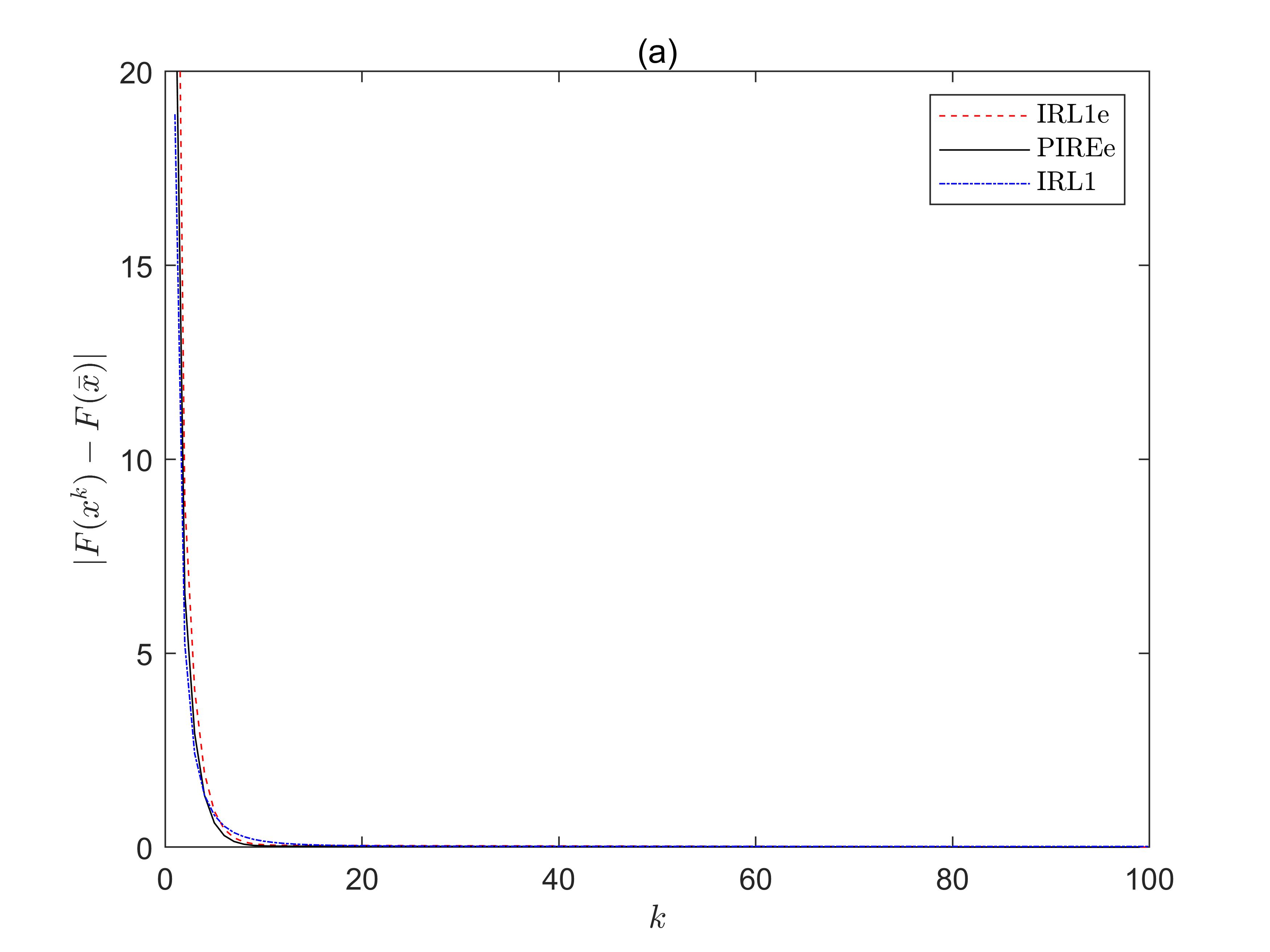
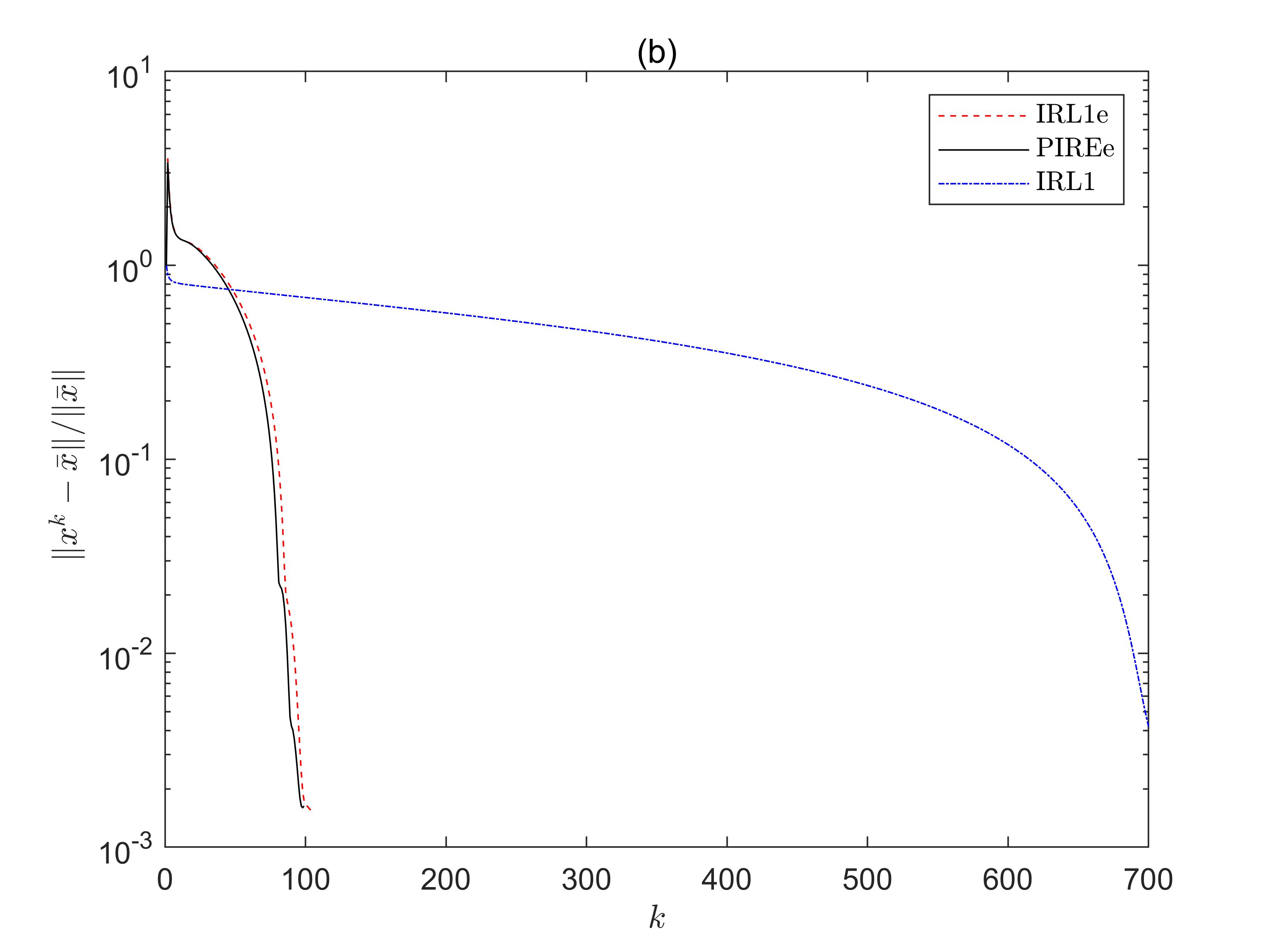
Figure 1: Numerical results when the sensing matrix $A$ is well-conditioned

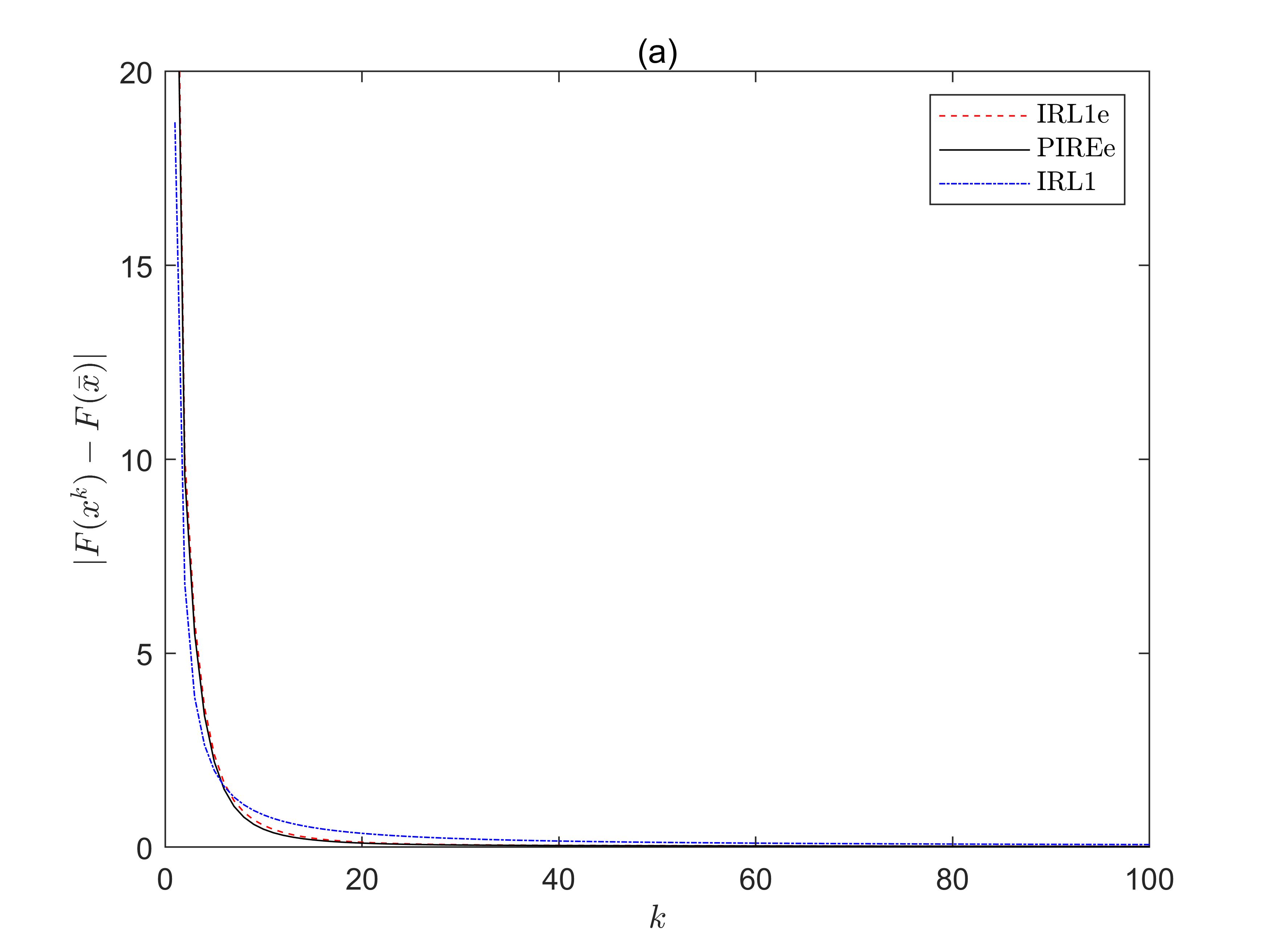
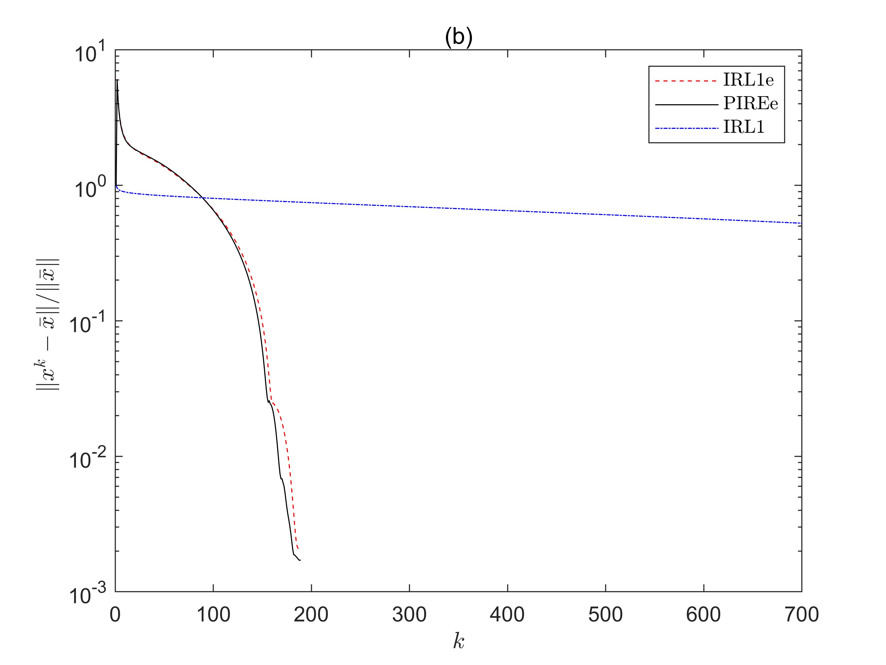
Figure 2: Numerical results when the sensing matrix $A$ is ill-conditioned

Table 1: Numerical results of PIREe, ${\rm{IRL_{1}e_{1}}}$ and ${\rm{IRL_{1}}}$

$A$	time			rel-err
	PIREe	${\rm{IRL_{1}e_{1}}}$	${\rm{IRL_{1}}}$	PIREe	${\rm{IRL_{1}e_{1}}}$	${\rm{IRL_{1}}}$
well-conditioned	0.86	0.92	3.83	1.71e-02	1.94e-02	2.13e-02
ill-conditioned	1.42	1.43	18.72	1.84e-02	2.14e-02	4.09e-02

Example 5.2.

We consider the following approximate $\ell_{q}$ optimization problem:

$$\min_{X\in\mathbb{R}^{q\times t}}F(X):=\frac{1}{2}\|AX-B\|^{2}_{F}+\sum_{i,j}(|X_{i,j}|+\varepsilon)^{p},\,0<p<1,$$ (41)

where $A\in\mathbb{R}^{n\times q}$, $B\in\mathbb{R}^{n\times t}$, $X=(X_{i,j})\in\mathbb{R}^{q\times t},i=1,\dots,q,\,j=1,\dots,t$.

In this example, $f(X)=\frac{1}{2}\|AX-B\|^{2}_{F}$, $h(y)=\lambda(y+\varepsilon)^{p}$, $g(t)=|t|$. The matrices $A,B$ are generated just like the well-conditioned case in the first example. We test the algorithm on two different sizes of data sets, i.e., $n=100,q=500,t=50$; $n=300,q=1000,t=200$. The corresponding blocks are set as $m=10$ and $m=20$, respectively. In each matrix column $X^{*}$, the sparsity is set as $0.02q$. The parameter $\lambda,\mu,q$ is chosen as $\lambda=0.015,\,\mu=0.1,\,p=0.1$. The extrapolation parameter is chosen as (40). The extrapolation parameter is set as zero if the objective function value is increasing at $k$th iteration and we do the iteration again.

We compare the proposed algorithm BPIREe with PIRE-AU and PIRE-PS [22]. The relative error is used as an evaluation metric which is defined as

$${\rm{rel.err.}}:=\frac{\|X^{k}-\bar{X}\|_{F}}{\|X^{k}\|_{F}}.$$

The stopping criterion is set as

$$\frac{\|X^{k+1}-X^{k}\|_{F}}{\|X^{k}\|_{F}}<10^{-4}.$$ (42)

The computational results are presented in Figures 3,4. The curves of $|F(X^{k})-F(\bar{X})|$ and $\|X^{k}-\bar{X}\|_{F}/\|\bar{X}\|_{F}$ against the number of the iterations are described respectively where $\bar{X}$ is the output of the proposed algorithm. From them, we see that the BPIREe algorithm outperforms PIRE-AU and PIRE-PS. In addition, we present the comparison results concerning the relative error and the used time of BPIREe, PIRE-AU, and PIRE-PS in Table 2. It is shown that the used time of the BPIREe algorithm is the least.

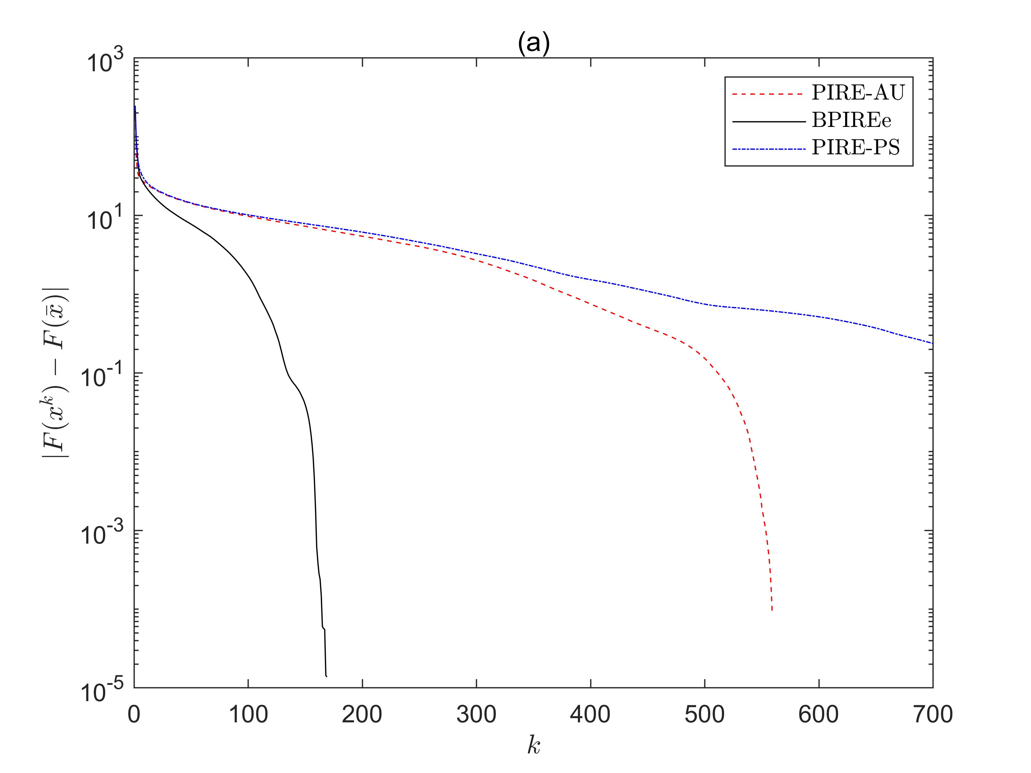
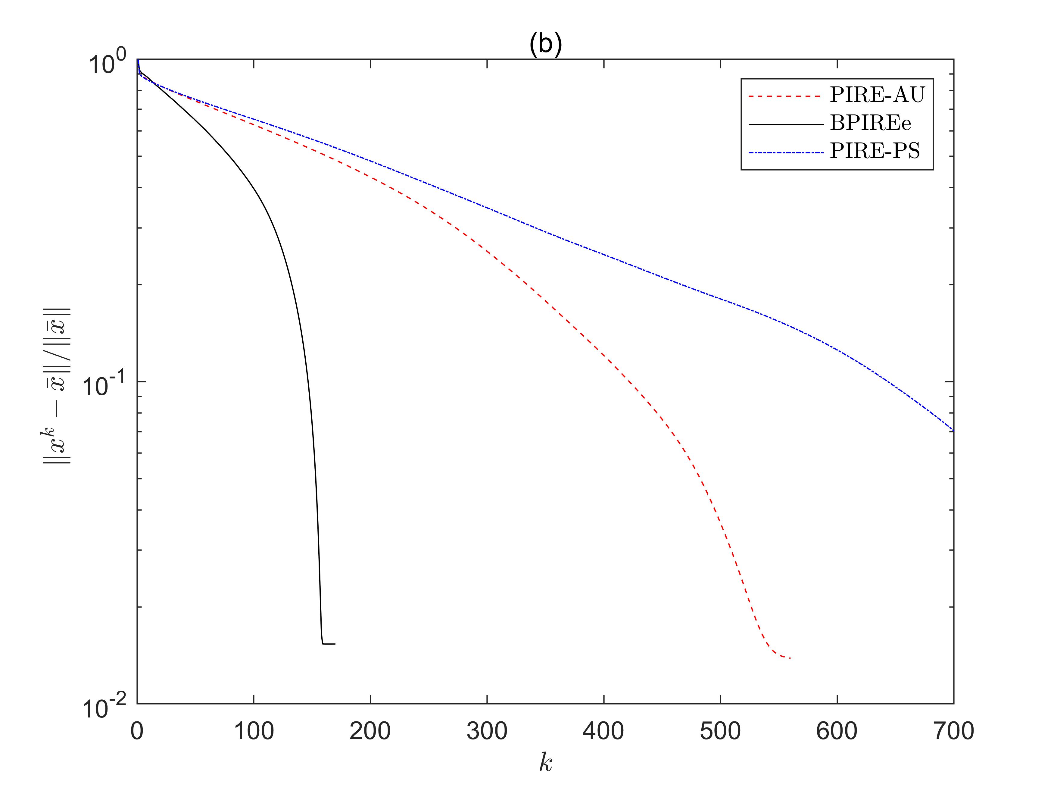
Figure 3: Numerical results when $n=100,q=500,t=50$

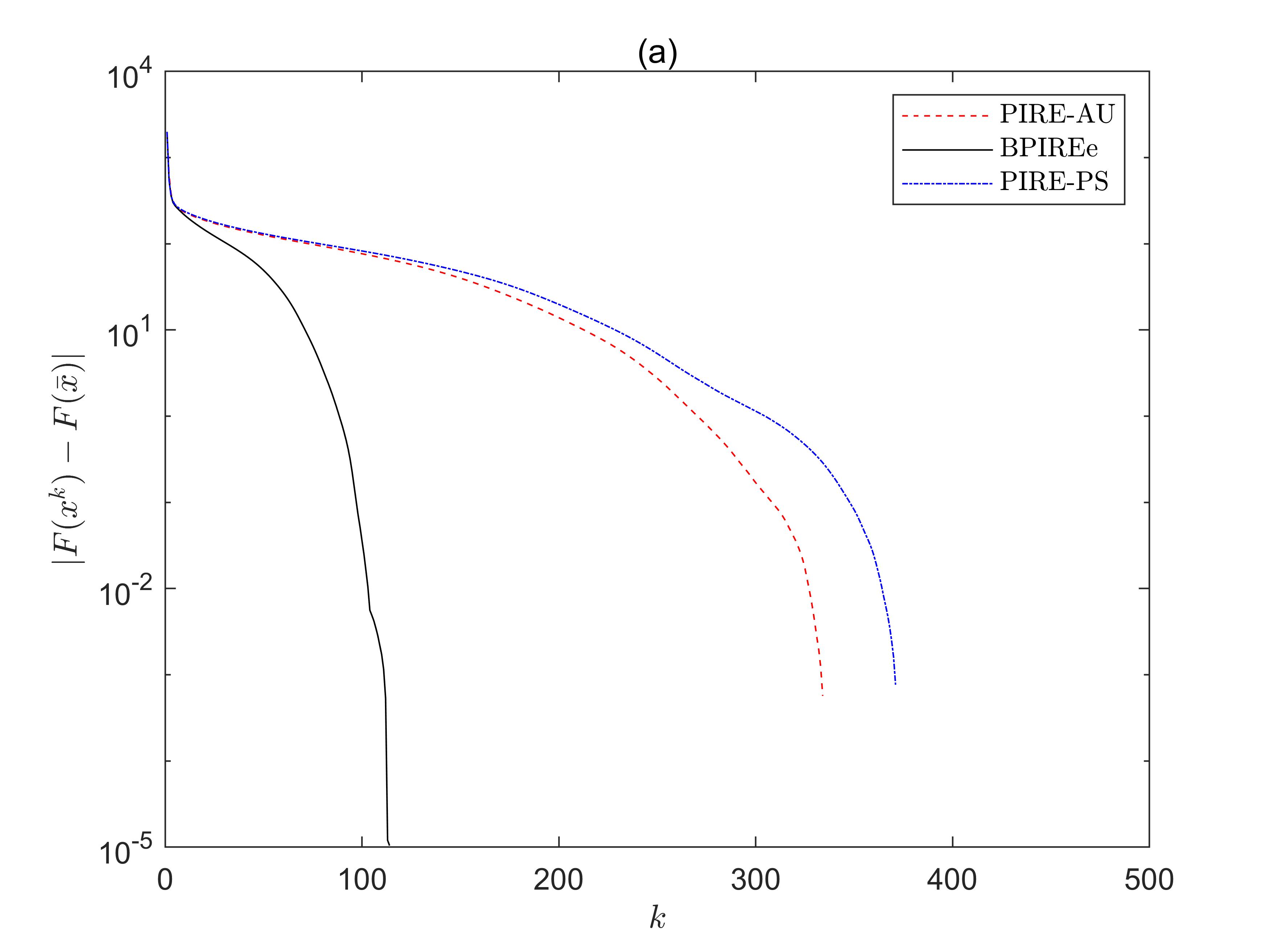
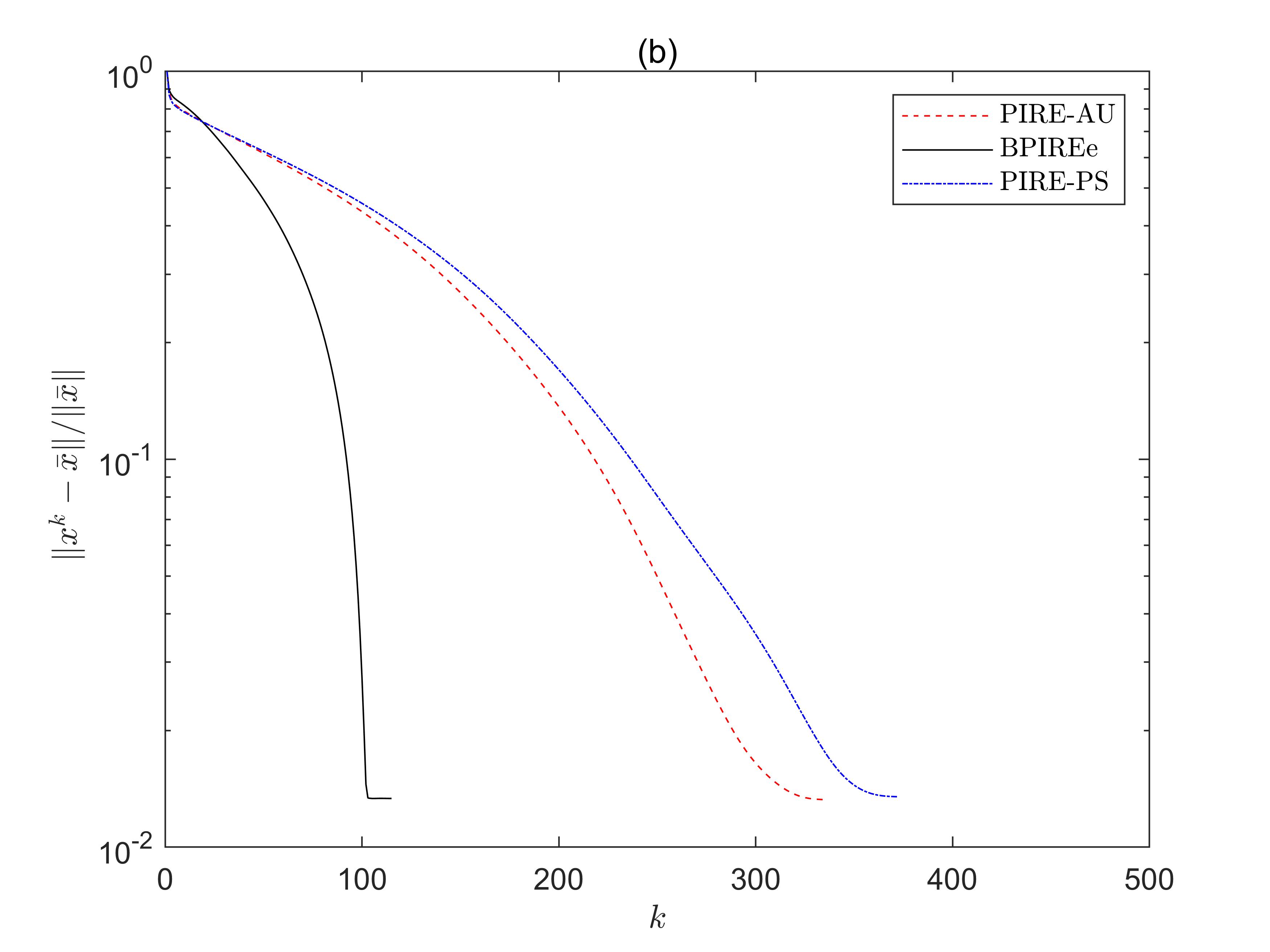
Figure 4: Numerical results when $n=300,q=1000,t=200$

Table 2: Numerical results of BPIREe, PIRE-AU and PIRE-PS

$m$	$n$	$t$	time			rel-err
			BPIREe	PIRE-AU	PIRE-PS	BPIREe	PIRE-AU	PIRE-PS
100	500	50	1.11	3.22	3.43	1.29e-02	1.44e-02	1.28e-02
300	1000	200	15.21	35.60	36.42	1.32e-02	1.33e-02	1.32e-02

6 Conclusions

We have developed a block proximal iteratively reweighted algorithm with extrapolation for solving a class of nonsmooth nonconvex problems. The proposed algorithm can be used to solve the $\ell_{p}$ regularization problem by employing a special adaptively updating strategy. There exists the non-zero extrapolation parameter that ensures the objective function is nonincreasing. We obtain the global convergence of the algorithm when the objective function satisfies the KL property. The numerical results illustrate that the extrapolation item speeds up the algorithm’s convergence, and the iterations and the used time are less than others.

Declarations

Confict of interest The authors declare that they have no con ict of interest.

Appendix A Appendix: Proof of Lemma 4.3

Suppose $a_{t}$ and $u_{t}$ be the vectors and their $i$th entries are

$$(a_{t})_{i}=\sqrt{\alpha_{i,\,n_{i,t}}},\,(u_{t})_{i}=A_{i,\,n_{i,t}}.$$

The inequality (33) can be rewritten as

$$\|a_{t+1}\odot u_{t+1}\|^{2}+(1-w^{2})\sum_{i=1}^{m}\sum_{j=n_{i,t}+1}^{n_{i,t+1}-1}\alpha_{i,j}A^{2}_{i,j}$$

$$\leq w^{2}\|a_{t}\odot u_{t}\|^{2}+B_{t}\sum_{i=1}^{m}\sum_{j=n_{i,t-1}+1}^{n_{i,t}}(A_{i,j}+C_{i,j-1}-C_{i,j}).$$ (43)

From the proof of Lemma 2 in [27], we get

$$\frac{1+w}{2}\|a_{t+1}\odot u_{t+1}\|+V_{1}\sum_{i=1}^{m}\sum_{j=n_{i,t}+1}^{n_{i,t+1}-1}A_{i,j}\leq\sqrt{\|a_{t+1}\odot u_{t+1}\|^{2}+\underline{\alpha}(1-w^{2})\sum_{i=1}^{m}\sum_{j=n_{i,t}+1}^{n_{i,t+1}-1}A^{2}_{i,j}},$$ (44)

where $V_{1}\leq\sqrt{\frac{\underline{\alpha}(1-w^{2})(4-(1+w)^{2})}{4mN}}$. Given $V_{2}>0$, we derive that

$$\sqrt{w^{2}\|a_{t}\odot u_{t}\|^{2}+B_{t}\sum_{i=1}^{m}\sum_{j=n_{i,t-1}+1}^{n_{i,t}}(A_{i,j}+C_{i,j-1}-C_{i,j})}$$

$$\leq w\|a_{t}\odot u_{t}\|+\sqrt{B_{t}\sum_{i=1}^{m}\sum_{j=n_{i,t-1}+1}^{n_{i,t}}(A_{i,j}+C_{i,j-1}-C_{i,j})}$$

$$\leq w\|a_{t}\odot u_{t}\|+\sqrt{B_{t}\sum_{i=1}^{m}\sum_{j=n_{i,t-1}+1}^{n_{i,t}}A_{i,j}}+\sqrt{B_{t}\sum_{i=1}^{m}\sum_{j=n_{i,t-1}+1}^{n_{i,t}}(C_{i,j-1}-C_{i,j})}$$

$$\leq w\|a_{t}\odot u_{t}\|+2V_{2}B_{t}+\frac{1}{4V_{2}}\sum_{i=1}^{m}\sum_{j=n_{i,t-1}+1}^{n_{i,t}}A_{i,j}+\frac{1}{4V_{2}}\sum_{i=1}^{m}\sum_{j=n_{i,t-1}+1}^{n_{i,t}}(C_{i,j-1}-C_{i,j})$$

$$\leq w\|a_{t}\odot u_{t}\|+2V_{2}B_{t}+\frac{1}{4V_{2}}\sum_{i=1}^{m}\sum_{j=n_{i,t-1}+1}^{n_{i,t}-1}A_{i,j}+\frac{1}{4V_{2}}\sum_{i=1}^{m}\sum_{j=n_{i,t-1}+1}^{n_{i,t}}(C_{i,j-1}-C_{i,j})+\frac{\sqrt{m}}{4V_{2}}\|u_{t}\|.$$ (45)

Together with (A), (44) and (A), we have

$$\frac{1+w}{2}\|a_{t+1}\odot u_{t+1}\|+V_{1}\sum_{i=1}^{m}\sum_{j=n_{i,t}+1}^{n_{i,t+1}-1}A_{i,j}$$

$$\leq w\|a_{t}\odot u_{t}\|+2V_{2}B_{t}+\frac{1}{4V_{2}}\sum_{i=1}^{m}\sum_{j=n_{i,t-1}+1}^{n_{i,t}-1}A_{i,j}+\frac{1}{4V_{2}}\sum_{i=1}^{m}\sum_{j=n_{i,t-1}+1}^{n_{i,t}}(C_{i,j-1}-C_{i,j})+\frac{\sqrt{m}}{4V_{2}}\|u_{t}\|$$

The rest of the proof is analogous to the Lemma 2 in [24], so we get the desired result.

References

[1]
H. Attouch, J. Bolte, and B. F. Svaiter, Convergence of descent methods for semi-algebraic and tame problems: proximal algorithms, forward-backward splitting, and regularized Gauss-Seidel methods, Math. Program. 137(1)(2013), pp. 91-129.
[2]
H. Attouch, J. Bolte, P. Redont, and A. Soubeyran, Proximal alternating minimization and projection methods for nonconvex problems: an approach based on the Kurdyka-Lojasiewicz
inequality, Math. Oper. Res. 35(2)(2010), pp. 438-457.
[3]
A. Auslender and M. Teboulle, Interior gradient and proximal methods for convex and conic optimization, SIAM J. Optim. 16(2006), pp. 697-725.
[4]
A. Beck and M. Teboulle, A fast iterative shrinkage-thresholding algorithm for linear inverse problems, SIAM J. Imaging Sci, 2(1)(2009), pp. 183-202.
[5]
J. Bolte, A. Daniilidis, and A. Lewis, The Łojasiewicz inequality for nonsmooth subanalytic functions with
applications to subgradient dynamical systems, SIAM J. Optim. 17(4)(2007), pp. 1205-1223.
[6]
J. Bolte, S. Sabach, and M. Teboulle,Proximal alternating linearized minimization for nonconvex and nonsmooth problems, Math. Program. 146 (2014), pp. 459-494.
[7]
E. J. Candes, M. B. Wakin, and S. P. Boyd, Enhancing sparsity by reweighted minimization, J. Fourier Anal. Appl., 14(5)(2008), pp. 877-905.
[8]
X. Chen, F. Xu, and Y. Ye, Lower bound theory of nonzero entries in solutions of minimization,
SIAM J. Sci. Comput. 32(2010), pp. 2832-2852.
[9]
I. Daubechies, R. DeVore, M. Fornasier, and C.S. Gunturk, Iteratively reweighted least squares minimization for sparse recovery, Commun. Pure. Appl. Math. 63(2010), pp. 1-38.
[10]
D. Drusvyatskiy and C. Paquette, Efficiency of minimizing compositions of convex functions and smooth maps, Math. Program. 178(1)(2019), pp. 503-558.
[11]
R. Chartrand and W. Yin, Iteratively reweighted algorithms for compressive sensing, In: 33rd International Conference on Acoustics, Speech, and Signal Processing (ICASSP) (2008).
[12]
S. Ghadimi and G. Lan, Accelerated gradient methods for nonconvex nonlinear and stochastic
programming, Math. Program. 156(2016), pp. 59-99.
[13]
K. Kurdyka, On gradients of functions definable in o-minimal structures, Annales de l’institut Fourier.
48(3)(1998), pp. 769-783.
[14]
G. Lan, Z. Lu, and R.D.C. Monteiro, Primal-dual first-order methods with iteration-complexity for cone programming, Math. Program. 126(2011), pp. 1-29.
[15]
C. Lu, Y. Wei, Z. Lin, and S. Yan, Proximal iteratively reweighted algorithm with multiple splitting for nonconvex sparsity optimization, In: Proceedings of the AAAI Conference on Artificial Intelligence
(2014).
[16]
Z. Lu, Iterative reweighted minimization methods for regularized unconstrained nonlinear programming, Math. Program. 147(1)(2014), pp. 277-307.
[17]
B. S. Mordukhovich, Variational analysis and generalized differentiation II: Applications[M], Springer, Berlin, 2006.
[18]
B. O’Donoghue, E.J. Cands, Adaptive restart for accelerated gradient schemes, Found. Comput.
Math. 15(2015), pp. 715-732.
[19]
R. T. Rockafellar, Convex Analysis, Princeton University Press, Princeton, 2015.
[20]
R. T. Rockafellar, and R. J. B. Wets, Variational Analysis, Springer, New York, 2009.
[21]
Y. Nesterov, Introductory lectures on convex programming volume i: Basic course,
Lecture notes, 3(4)(1998).
[22]
T. Sun, H. Jiang, and L. Cheng, Global convergence of proximal iteratively reweighted algorithm, J. Global Optim. 68(4)(2017), pp. 815-826.
[23]
P. Tseng, Approximation accuracy, gradient methods, and error bound for structured
convex optimization, Math. Program. 125(2)(2010), pp. 263-295.
[24]
H. Wang, H. Zeng , and J. Wang, An extrapolated iteratively reweighted method with complexity analysis, Comput. Optim. Appl. (2022), pp. 1-31.
[25]
H. Wang, H. Zeng, and J. Wang, Relating regularization and reweighted regularization, Optim. Lett. (2021), pp. 1-22.
[26]
Y. Xu and W. Yin, A block coordinate descent method for regularized multiconvex optimization with
applications to nonnegative tensor factorization and completion, SIAM J. Imaging Sci. 6(3)(2013), pp. 1758-1789.
[27]
Y. Xu and W. Yin, A Globally Convergent Algorithm for Nonconvex Optimization Based on Block Coordinate Update, J. Sci. Comput. 72(2)(2017), pp. 700-734.
[28]
P. Yu and T. K. Pong, Iteratively reweighted algorithms with extrapolation, Comput. Optim. Appl. 73(2)(2019), pp. 353-386.