The convergence rate of the accelerated proximal gradient algorithm for Multiobjective Optimization is faster than $O(1/k^{2})$

Abstract

In this paper, we propose a fast proximal gradient algorithm for multiobjective optimization, it is proved that the convergence rate of the accelerated algorithm for multiobjective optimization developed by Tanabe et al. can be improved from $O(1/k^{2})$ to $o(1/k^{2})$ by introducing different extrapolation term $\frac{k-1}{k+\alpha-1}$ with $\alpha>3$. Further, we establish the inexact version of the proposed algorithm when the error term is additive, which owns the same convergence rate. At last, the efficiency of the proposed algorithm is verified on some numerical experiments.

1 Introduction

We mainly focus on the multiobjective optimization,

$$\min\limits_{x\in\mathbb{R}^{n}}F(x)$$ (1)

with $F:\mathbb{R}^{n}\to(\mathbb{R}\cup\{\infty\})^{m}$ and $F:=(F_{1},\dots,F_{m})^{T}$ taking the form

$$F_{i}(x):=f_{i}(x)+g_{i}(x),\,i=1,2,\dots,m,$$ (2)

where $f_{i}:\mathbb{R}^{n}\to\mathbb{R}$ is a convex and continuously differentiable function and $g_{i}:\mathbb{R}^{n}\to(-\infty,+\infty]$ is a closed, proper and convex function. Suppose the gradient $\nabla f_{i}(x)$ of $f_{i}(x)$ in (2) is Lipschitz continuous with $L_{i}$ and let

$$L:=\max_{i=1,\dots,m}L_{i},$$

Multiobjective optimization refers to the process of simultaneously minimizing (or maximizing) multiple objective functions while taking into account any relevant constraints. In most cases, it is not possible to find a single point that minimizes all objective functions at the same time, making the concept of Pareto optimality indispensable. A point is deemed Pareto optimal or efficient if there is no other point with equal or lower objective function values, and at least one objective function value is strictly lower. The applications of multi-objective optimization span across diverse domains, and for an extensive list of examples, please refer to Beck ; Boyd .

Recently, the descent methods for multiobjective optimization problems,

Various first-order methods, including steepest descent types,Fliege2 , projected gradient methods,Fliege2 , proximal point methods,Fukuda , conjugate gradient methods,Lucambio , Barzilai-Borwein descent methods,ChenJian , and conditional gradient methods,chenw , have garnered significant attention and extensive research efforts. These methods are widely studied for optimization tasks. In addition to first-order approaches, second-order methods such as the Newton method,Fliege1 , trust region methods,Carrizo , and Newton-type proximal gradient methods,Ansary have been explored. These second-order methods leverage information about the curvature of the objective function, making them more efficient for certain optimization problems but potentially more computationally expensive.

When $m=1$, the multiobjective optimization problem (MOP) (1) reduces to the single objective case,

$$\min\limits_{x\in\mathbb{R}^{n}}F(x):=f(x)+g(x).$$ (3)

The proximal gradient (PG) algorithm is a popular method to solve the composition optimization problem especially when the proximal operator of $g$ has an explicit solution. However, the convergence rate $O(1/k)$ of the proximal gradient method is slow. Lots of researchers devote to improve the efficiency of the PG algorithm. In 2009, Beck and Teboulle Beck developed the remarkble Fast Iterative Shrinkage Thresholding Algorithm (FISTA) for the convex case. The convergence rate $O(1/k^{2})$ of the objective function is obtained. Moreover, Chambolle and Dossal Chambolle gave the modification version of the FISTA and further obtained the sequence convergence of proposed algorithm.It is worth noting that Attouch and Peypouquet Attouch introduced an extrapolation technique, specifically $\frac{k-1}{k+\alpha-1}$ with $\alpha>3$, into the proximal gradient method for solving (3). This innovation led to an enhanced convergence rate, improving from $O(1/k^{2})$ to $o(1/k^{2})$.

The accelerated algorithm mentioned above does not leverage additional second-order information at a higher computational cost. Despite this, it achieves an enhanced convergence rate. Inspired by the benefit of acceleration algorithms on single-objective scenarios, the researchers are increasingly focusing on the study of acceleration algorithms in multi-objective optimization problems. Recently, Tanabe et al. Tanabe1 extends the remarkable FISTA to the multiobjective case and the convergence rate $O(1/k^{2})$ characterized by merit function Tanabe is obtained which improved the proximal gradient method for MOP Tanabe3 . Nishimura et al. Nishimura established the monotonicity version of the multiobjective FISTA. Moreover, Tanabe et al. Tanabe4 generalizes the multiobjective FISTA by introducing some hyperparameters which is also a generalization even in the single-objective case and preserves the same convergence rate $O(1/k^{2})$ as multiobjective FISTA. Besides, it is proved that the iterative sequences is convergent.

Based on the fast algorithms in single-objective case proposed by Attouch Attouch , we introduce the extrapolation parameter $\frac{k-1}{k+\alpha-1}$ with $\alpha>3$ into the multiobjective proximal gradient algorithm. The convergence rate described by the merit function achives $o(1/k^{2})$ which improves the multiobjective FISTA Tanabe1 . Along with we get the sequence convergence of the iterations. Additionaly, the inexact version of the proposed algorithm is also got when the errors satisfying some additivity and the convergence rate remains unchanged.

The organization of the paper is as follows. Some notations and definitions are given in Sect. 2. Sect. 3 presents the algorithm framework of fast proximal gradient algorithm for multi-objective optimization. Sect. 4 focus on proving the convergence of the proposed algorithm. Numerical results are presented in Sect. 5, which demonstrates that the proposed algorithm exhibits rapid convergence effects. Towards the conclusion of the paper, several key conclusions are presented.

2 Preliminary Results

For convenience, we present some notations and definitions which used in the overall paper. Denote $\mathbb{R}^{n}$ be the $n$-dimensional space, and $\mathbb{R}^{n}_{+}:=\{v\in\mathbb{R}^{n}|v_{i}\geq 0,i=1,2,\dots,n\}$; $\triangle^{n}$ be the standard simplex in $\mathbb{R}^{n}$ with

$$\triangle^{n}:=\left\{\lambda\in\mathbb{R}^{n}_{+}\bigg{|}\lambda_{i}\geq 0,\sum_{i=1}^{n}\lambda_{i}=1.\right\}$$

The Euclidean norm defined in $\mathbb{R}^{n}$ is $\|u\|:=(\sum_{i=1}^{n}u^{2}_{i})^{1/2}$ for $u\in\mathbb{R}^{n}$.

The partial orders induced by $\mathbb{R}^{n}_{+}$ implies that for any $v^{1},v^{2}\in\mathbb{R}^{n}_{+}$, if $v^{2}-v^{1}\in\mathbb{R}^{n}_{+}$, then $v^{1}\leq v^{2}$ and if $v^{2}-v^{1}\in{\rm int}\mathbb{R}^{n}_{+}$, then $v^{1}<v^{2}$.

For a closed, proper and convex function $h:\mathbb{R}^{n}\to\mathbb{R}\cup\{\infty\}$, the Moreau envelope of $h$ defined by

$$\mathcal{M}_{h}(x):=\min_{y\in\mathbb{R}^{n}}\left\{h(y)+\frac{1}{2}\|x-y\|^{2}\right\}$$

The unique solution of the above problem is called the proximal operator of $h$, which is denoted as

$${\rm prox}_{h}(x):=\arg\min_{y\in\mathbb{R}^{n}}\left\{h(y)+\frac{1}{2}\|x-y\|^{2}\right\}.$$

Lemma 1.

Beck If $h$ is a proper closed and convex function, the Moreau envelope $\mathcal{M}_{h}$ is 1-Lipschitz continuous and its gradient takes the following form,

$$\nabla\mathcal{M}_{h}(x):=x-{\rm prox}_{h}(x).$$

Next we recall the optimality concept for the multiobjective optimization problem (1): $x^{*}\in\mathbb{R}^{n}$ is weakly pareto optimal if there no exist $x\in\mathbb{R}^{n}$ such that $F(x)<F(x^{*})$. Denote the set of weakly pareto optimal solutions be $X^{*}$.

The merit function $u_{0}:\mathbb{R}^{n}\to\mathbb{R}\cup\{\infty\}$ given in Tanabe takes the following form

$$u_{0}(x):=\sup\limits_{z\in\mathbb{R}^{n}}\min_{i=1,\dots,m}[F_{i}(x)-F_{i}(z)],$$ (4)

and proves that $u_{0}$ is a merit function in the Pareto sense.

Lemma 2.

Tanabe Let $u_{0}$ be given as (4), then $u_{0}(x)\geq 0$, $x\in\mathbb{R}^{n}$, and $x$ is the weakly Pareto optimal for (1) if and only if $u_{0}(x)=0$.

3 The fast proximal gradient algorithm for multi-objective optimization

In this section, we propose the fast proximal gradient algorithm for multi-objective optimization. The subproblem has the same form in Tanabe , in detail, for $x\in domF,\,\ell>L$,

$$\min_{z\in\mathbb{R}^{n}}\phi_{\ell}(z;x,y)$$ (5)

where

$$\phi_{\ell}(z;x,y):=\max\limits_{i=1,\dots,m}\left\{\langle\nabla f_{i}(y),z-y\rangle+g_{i}(z)+f_{i}(y)-F_{i}(x)\right\}+\frac{\ell}{2}\|z-y\|^{2}.$$ (6)

Define

$$p_{\ell}(x,y):=\arg\min\limits_{z\in\mathbb{R}^{n}}\phi_{\ell}(z;x,y),\quad\theta_{\ell}(x,y):=\min_{z\in\mathbb{R}^{n}}\phi_{\ell}(z;x,y)$$ (7)

The optimality condition of (5) means that there exists $\eta(x,y)\in\partial g(p_{\ell}(x,y))$ and the Lagrange multiplier $\lambda(x,y)\in\mathbb{R}^{m}$ satisfying

$$\sum_{i=1}^{m} \lambda_{i}(x,y)\{\nabla f_{i}(y)+\eta_{i}(x,y)\}=-\ell(p_{\ell}(x,y)-y)$$ (8)

$$\lambda(x,y)\in\triangle^{m},\lambda_{i}(x,y)=0,i\notin\mathcal{I}(x,y),$$ (9)

where $\triangle^{m}$ represents the standard simplex and

$$\mathcal{I}(x,y):=\arg\max\limits_{i=1,\cdots,m}\left\{\langle\nabla f_{i}(y),z-y\rangle+g_{i}(z)+f_{i}(y)-F_{i}(x)\right\}+\frac{\ell}{2}\|z-y\|^{2}.$$

Lemma 3.

Tanabe1 Suppose $p_{\ell}(x,y)$ is defined as in (7), then $y\in\mathbb{R}^{n}$ is the weakly Pareto optimal for (1) if and only if $p_{\ell}(x,y)=y$ for some $x\in\mathbb{R}^{n}$.

The result implies that it is allowable to use $\|p^{acc}_{\ell}(x,y)-y\|_{\infty}$ as the stopping criterion of the corresponding fast proximal gradient algorithm for MOP. The specific algorithm framework is as follows.

Algorithm 1 The Fast Proximal Gradient Algorithm for Multi-objective Optimization

1:  Initialization: Give a starting point $x^{0}=y^{1}\in domF$, $\alpha>3$, $\varepsilon>0$. Set $k=0$.

2:  while  $\|p_{\ell}(x^{k-1},y^{k})-y^{k}\|\geq\varepsilon$ do

3:     

$$x^{k}\to p_{\ell}(x^{k-1},y^{k}),$$

4:     

$$y^{k+1}=x^{k}+\frac{k-1}{k+\alpha-1}(x^{k}-x^{k-1}),$$ (10)

5:     $k\to k+1$.

6:  end while

4 The convergence rate analysis of FPGMOP for (1).

Given a fixed weakly pareto solution $x^{*}\in\mathbb{R}^{n}$, define the auxiliary sequence

$$\mathscr{E}_{k+1}:=\frac{2(k+\alpha-1)^{2}}{\ell(\alpha-1)}\sigma_{k+1}+(\alpha-1)\|u^{k+1}-x^{*}\|^{2}.$$ (11)

where $\sigma_{k+1}:=\sigma_{k+1}(x^{*})=\min\limits_{i=1,\cdots,m}\left\{F_{i}(x^{k})-F_{i}(x^{*})\right\}$, $u^{k+1}:=\frac{k+\alpha-1}{\alpha-1}x^{k+1}-\frac{k}{\alpha-1}x^{k}$.

Lemma 4.

Tanabe1 Suppse $\{x^{k}\}$ and $\{y^{k}\}$ are the sequences genetated by Algorithm1, it holds that for any $k\geq 0$

$$\sigma_{k+1}(z)\leq\frac{-\ell}{2}\left\{2\langle x^{k+1}-y^{k+1},y^{k+1}-z\rangle+\|x^{k+1}-y^{k+1}\|^{2}\right\}-\frac{\ell-L}{2}\|x^{k+1}-y^{k+1}\|^{2},$$ (12)

and

$$\sigma_{k}(z)-\sigma_{k+1}(z)\geq\frac{\ell}{2}\left\{2\langle x^{k+1}-y^{k+1},y^{k+1}-x^{k}\rangle+\|x^{k+1}-y^{k+1}\|^{2}\right\}+\frac{\ell-L}{2}\|x^{k+1}-y^{k+1}\|^{2},$$ (13)

where $\sigma_{k}(z)=\min\limits_{i=1,\cdots,m}\left\{F_{i}(x^{k})-F_{i}(z)\right\}$.

Theorem 1.

Suppose $\{x^{k}\}$ and $\{y^{k}\}$ be the sequences genetated by Algorithm1, for any $z\in\mathbb{R}^{n}$, $k\geq 0$ and $\alpha>3$, it holds that

1. $\mathscr{E}_{k+1}\leq M:=\frac{2(\alpha-1)}{l}\|x^{0}-x^{*}\|^{2}.$

2. $\sum_{k=0}^{+\infty}(k+\alpha-1)\sigma_{k}(z)\leq\frac{\ell M(\alpha-1)}{\alpha-3};$

3. $\sum_{k=0}^{+\infty}k\|x^{k+1}-x^{k}\|^{2}\leq\frac{3\ell(\alpha-1)M}{(\alpha-3)};$

4. $\lim_{{k\to+\infty}}k^{2}\|x^{k+1}-x^{k}\|^{2}+(k+1)^{2}\sigma_{k}\quad\text{\rm exists};$

5. $u_{0}(x^{k})=o(1/k^{2})\quad\text{\rm and}\quad\|x^{k+1}-x^{k}\|=o(1/k).$

Proof. (i) Accoring to Lemma 4, multiplying (12) by $\frac{\alpha-1}{k+\alpha-1}$ and (13) by $\frac{k}{k+\alpha-1}$ and adding them together, it holds that

$$\sigma_{k+1}(z)-\frac{k}{k+\alpha-1}\sigma_{k}(z)\leq\ell\left\{\langle y^{k+1}-x^{k+1},y^{k+1}-\frac{k}{k+\alpha-1}x^{k}-\frac{\alpha-1}{k+\alpha-1}z\rangle\right\}$$

$$-\frac{\ell}{2}\|x^{k+1}-y^{k+1}\|^{2}-\frac{\ell-L}{2}\|x^{k+1}-y^{k+1}\|^{2},$$

It is noted that

$$-\|x^{k+1}-y^{k+1}\|^{2}+2\langle y^{k+1}-x^{k+1},y^{k+1}-\frac{k}{k+\alpha-1}x^{k}-\frac{\alpha-1}{k+\alpha-1}z\rangle$$

$$= -\|x^{k+1}-\frac{k}{k+\alpha-1}x^{k}-\frac{\alpha-1}{k+\alpha-1}z\|^{2}+\|y^{k+1}-\frac{k}{k+\alpha-1}x^{k}-\frac{\alpha-1}{k+\alpha-1}z\|^{2}$$

$$= -(\frac{\alpha-1}{k+\alpha-1})^{2}(\|u^{k+1}-z\|^{2}-\|u^{k}-z\|^{2})$$

where $u^{k}:=\frac{k+\alpha-2}{\alpha-1}x^{k}-\frac{k-1}{\alpha-1}x^{k-1}$. Then we get

$$\sigma_{k+1}(z)-\frac{k}{k+\alpha-1}\sigma_{k}(z)\leq-\frac{\ell}{2}(\frac{\alpha-1}{k+\alpha-1})^{2}(\|u^{k+1}-z\|^{2}-\|u^{k}-z\|^{2})-\frac{\ell-L}{2}\|x^{k+1}-y^{k+1}\|^{2},$$

Multiplying the above inequality by $\frac{2(k+\alpha-1)^{2}}{\ell(\alpha-1)}$, it yields that

$$\mathscr{E}_{k+1}\leq\frac{2k(k+\alpha-1)}{\ell(\alpha-1)}\sigma_{k}(z)+(\alpha-1)\|u^{k}-z\|^{2}-\frac{(\ell-L)(k+\alpha-1)^{2}}{\ell(\alpha-1)}\|x^{k+1}-y^{k+1}\|^{2}.$$

Since $k(k+\alpha-1)<(k+\alpha-2)^{2}-(\alpha-3)(k+\alpha-1)$, we get

$$\mathscr{E}_{k+1}+\frac{2(\alpha-3)(k+\alpha-1)}{\ell(\alpha-1)}\sigma_{k}(z)\leq\mathscr{E}_{k}-\frac{(\ell-L)(k+\alpha-1)^{2}}{\ell(\alpha-1)}\|x^{k+1}-y^{k+1}\|^{2}\leq\mathscr{E}_{k},$$ (14)

Then the sequence $\{\mathscr{E}_{k}\}$ is nonincreasing. Moreover, from (11) and $\sigma_{k}(z)\geq 0$, it yields that $\mathscr{E}_{k}$ is lower-bounded and $\lim_{k\to+\infty}\mathscr{E}_{k}$ exists and ${\mathscr{E}_{k}}\leq{\mathscr{E}_{1}}$ for $k\geq 0$ .

From (12), we have

$$\sigma_{1} \leq\frac{-\ell}{2}\left\{2\langle x^{1}-y^{1},y^{1}-x^{*}\rangle+\|x^{1}-y^{1}\|^{2}\right\}-\frac{\ell-L}{2}\|x^{1}-y^{1}\|^{2},$$

$$\leq\frac{-\ell}{2}\left\{2\langle x^{1}-y^{1},y^{1}-x^{*}\rangle+\|x^{1}-y^{1}\|^{2}\right\}$$

$$\leq\frac{\ell}{2}(-\|x^{1}-x^{*}\|^{2}+\|y^{1}-x^{*}\|^{2})=\frac{\ell}{2}(-\|x^{1}-x^{*}\|^{2}+\|x^{0}-x^{*}\|^{2})$$

Combining this with $\mathscr{E}_{1}=\frac{2(\alpha-1)}{l}\sigma_{1}+(\alpha-1)\|x^{1}-x^{*}\|^{2}$, we get

$${\mathscr{E}_{1}}\leq\frac{2(\alpha-1)}{l}\|x^{0}-x^{*}\|^{2},$$

i.e.,for any $k\geq 0$, it holds that

$$\mathscr{E}_{k+1}\leq\frac{2(\alpha-1)}{l}\|x^{0}-x^{*}\|^{2}.$$

So the result (i) hold.

(ii) Summing up the inequality (14) from $k=1$ to $k=K$, we get

$$\mathscr{E}_{K+1}+\sum_{k=1}^{K}\frac{(\alpha-3)(k+\alpha-1)}{\ell(\alpha-1)}\sigma_{k}(z)\leq\mathscr{E}_{1}.$$ (15)

From (15), we have

$$\sum_{k=0}^{K}\frac{(\alpha-3)(k+\alpha-1)}{\ell(\alpha-1)}\sigma_{k}(z)\leq\mathscr{E}_{1}-\mathscr{E}_{K+1}.$$

Letting $K\to+\infty$, due to $\mathscr{E}_{K+1}\leq\mathscr{E}_{1}$ and $\lim_{k\to\infty}\mathscr{E}_{k+1}$ exists, we get

$$\sum_{k=0}^{+\infty}(k+\alpha-1)\sigma_{k}(z)\leq\frac{\ell\mathscr{E}_{1}(\alpha-1)}{\alpha-3},$$

so the result (ii) holds.

(iii) According to (13) and the Pythagoras relation

$$\|b-a\|^{2}+2\langle b-a,a-c\rangle=\|b-c\|^{2}-\|a-c\|^{2}$$ (16)

with $(a,b,c)=(y^{k+1},x^{k+1},x^{k})$, we have

$$\sigma_{k+1}(z)-\sigma_{k}(z) \leq\frac{\ell}{2}\left\{-\|x^{k+1}-x^{k}\|^{2}+\|y^{k+1}-x^{k}\|^{2}\right\}-\frac{\ell-L}{2}\|x^{k+1}-y^{k}\|^{2}$$

$$=\frac{\ell}{2}\left\{-\|x^{k+1}-x^{k}\|^{2}+(\frac{k-1}{k+\alpha-1})^{2}\|x^{k}-x^{k-1}\|^{2}\right\}$$

$$\quad-\frac{\ell-L}{2}\|x^{k+1}-x^{k}-\frac{k-1}{k+\alpha-1}(x^{k}-x^{k-1})\|^{2}$$

$$=-\frac{2\ell-L}{2}\|x^{k+1}-x^{k}\|^{2}+\frac{L}{2}(\frac{k-1}{k+\alpha-1})^{2}\|x^{k}-x^{k-1}\|^{2}$$

$$\quad+(\ell-L)\langle x^{k+1}-x^{k},\frac{k-1}{k+\alpha-1}(x^{k}-x^{k-1})\rangle$$

$$\leq-\frac{\ell}{2}\|x^{k+1}-x^{k}\|^{2}+\frac{\ell}{2}(\frac{k-1}{k+\alpha-1})^{2}\|x^{k}-x^{k-1}\|^{2},$$ (17)

where the last inequaltiy holds due to the Caucy-Schwarz inequality.

The subsequent analysis is similar to (17) in Attouch , for completeness, a detailed derivation is given below. From (4) and $k+\alpha-1\geq k+1$, it holds that

$$(k+1)^{2}d_{k}-(k-1)^{2}d_{k-1}\leq(k+1)^{2}(\sigma_{k}(z)-\sigma_{k+1}(z)),$$

where $d_{k}=\frac{\ell}{2}\|x^{k+1}-x^{k}\|^{2}$. Since

$$(k+1)^{2}(\sigma_{k}(z)-\sigma_{k+1}(z)) =k^{2}\sigma_{k}(z)-(k+1)^{2}\sigma_{k+1}(z)+(2k+1)\sigma_{k}(z)$$

$$\leq k^{2}\sigma_{k}(z)-(k+1)^{2}\sigma_{k+1}(z)+3k\sigma_{k}(z),$$

we get

$$2kd_{k}+k^{2}d_{k}-(k-1)^{2}d_{k-1}\leq (k+1)^{2}d_{k}-(k-1)^{2}d_{k-1}$$

$$\leq (k+1)^{2}(\sigma_{k}(z)-\sigma_{k+1}(z))$$

$$\leq k^{2}\sigma_{k}(z)-(k+1)^{2}\sigma_{k+1}(z)+3k\sigma_{k}(z).$$

Summing the inequality from $k=1$ to $K$, we have

$$K^{2}d_{K}+2\sum_{k=0}^{K}kd_{k}\leq\sigma_{1}+\frac{3\ell(\alpha-1)\mathscr{E}_{1}}{2(\alpha-3)},\quad K\in\mathbb{N},$$

and so

$$\sum_{k=0}^{+\infty}k\|x^{k+1}-x^{k}\|^{2}\leq\frac{3\ell(\alpha-1)\mathscr{E}_{0}}{(\alpha-3)}.$$

(iv) Similar to the analysis of Lemma 2 in Attouch , the desired results can be obtained.

(v) From (6) and the result (iv), it can be easily got.

In the following, we are ready to prove the convergence of the iterations. Now we first recall two lemmas which will be used in the later.

Lemma 5.

Opial (Opial’s lemma) Let $S\subset\mathbb{R}^{n}$ be a nonempty set, if the sequence $\{z^{k}\}$ satisfies the following

1. ${\rm lim}_{k\to+\infty}\|z_{k}-z\|$ exists for every $z\in S$,

2. every limit point of the sequence $\{z_{k}\}$ is in the set $S$,

then the sequence $\{z^{k}\}$ convergence to a point in $S$.

Lemma 6.

Attouch Suppose $\alpha>3$ and nonegative sequences $\{a_{k}\}$ and $\{w_{k}\}$ satisfy

$$a_{k+1}\leq\frac{k-1}{k+\alpha-1}a_{k}+w_{k},$$

and $\sum_{k=1}^{\infty}kw_{k}<\infty,$ then $\sum_{k=1}^{\infty}a_{k}<\infty.$

Theorem 2.

Suppose $\{x^{k}\}$ is the sequence generated by algorithm 1, then the sequence gerenrated by the algorithm 1 is weakly Pareto optimal for (1).

Proof. Based on the Lemma 2 and Theorem 1, we just need to prove that the sequence $\{x^{k}\}$ generated by the algorithm 1 convergences. Since $\sigma_{k+1}(x^{*})\geq 0$, $x^{*}\in X^{*}$, from (12), we get

$$2\langle y^{k+1}-x^{k+1},y^{k+1}-x^{*}\rangle-\|x^{k+1}-y^{k+1}\|^{2}\geq 0,$$

that is

$$\|y^{k+1}-x^{*}\|^{2}-\|x^{k+1}-x^{*}\|^{2}\geq 0.$$

Then

$$\|x^{k+1}-x^{*}\|^{2}$$

$$\leq \|y^{k+1}-x^{*}\|^{2}$$

$$= \|x^{k}-x^{*}\|^{2}+(\frac{k-1}{k+\alpha-1})^{2}\|x^{k}-x^{k-1}\|^{2}+2(\frac{k-1}{k+\alpha-1})\langle x^{k}-x^{*},x^{k}-x^{k-1}\rangle$$

$$= \|x^{k}-x^{*}\|^{2}+((\frac{k-1}{k+\alpha-1})^{2}+\frac{k-1}{k+\alpha-1})\|x^{k}-x^{k-1}\|^{2}$$

$$\quad+\frac{k-1}{k+\alpha-1}(\|x^{k}-x^{*}\|^{2}-\|x^{k-1}-x^{*}\|^{2})$$

$$\leq \|x^{k}-x^{*}\|^{2}+2\|x^{k}-x^{k-1}\|^{2}++\frac{k-1}{k+\alpha-1}(\|x^{k}-x^{*}\|^{2}-\|x^{k-1}-x^{*}\|^{2})$$

Let $h_{k}:=\|x^{k}-x^{*}\|^{2}$, then we have

$$(h_{k+1}-h_{k})_{+}\leq(\frac{k-1}{k+\alpha-1})(h_{k}-h_{k-1})_{+}+2\|x^{k}-x^{k-1}\|^{2},$$

According to Theorem1(iii) and Lemma 6, we get $\sum_{k=1}^{\infty}(h_{k+1}-h_{k})_{+}<\infty,$ and further we have $\lim_{k\to\infty}h_{k}$ exists by the nonegative of $\{h_{k}\}$.

Remark 1.

Recently, it is observed that the fast multiobjective gradient methods with Nesterov acceleration also proposed through the inertial gradient-like dynamical systems Sonntag1 ; Sonntag2 . In Sonntag1 , the authors considered the problem (1) with $h(x)=0$ and established the inertial first order method for MOP by an discretization of the differential equation. Further, they proved the convergence rate characterised by the merit function is $O(1/k^{2})$ just when the extrapolation parameter $\beta_{k}=\frac{k-1}{k+2}$ which is the special case of (10); this algorithm has the similar convergence behaviors to the accelerated algorithm given by Tanabe1 which has been discussed in Sonntag1 . However, the convergence rate of the accelerated proximal gradient algorithms when $\alpha>3$ has not been obtained both in the discrete case Sonntag1 and the continuous case Sonntag2 . This question also was raised as an open question in the Section 9 of Sonntag1 . Fortunately, based on the Lemma 6.3, Lemma 6.5 in Sonntag1 and motivated by the Theorem 1, we also can obtain that the convergence rate $o(1/k^{2})$ also can be obtained when $\alpha>3$ in the fast proximal gradient algorithm for MOP Sonntag1 which solved their open question Sonntag1 .

5 Stability

In this part, we consider the inexact version of the Algorithm 1, the inexact error mainly comes from to the calculation of the $\nabla f_{i}(x)$, in detail, the subproblem in (5) takes the following form,

$${\hat{\phi}}_{\ell}(z;x,y,\epsilon):=\max\limits_{i=1,\dots,m}\left\{\langle\nabla f_{i}(y)+\epsilon,z-y\rangle+g_{i}(z)+f_{i}(y)-F_{i}(x)\right\}+\frac{L}{2}\|z-y\|^{2},$$ (18)

where $\epsilon\in\mathbb{R}^{n}$ is the unknown error. The corresponding optimality condition yields that there exists ${\hat{\eta}}(x,y,\epsilon)\in\partial g(\hat{p}_{\ell}(x,y,\epsilon))$ and the Lagrange multiplier ${\hat{\lambda}}(x,y,\epsilon)\in\mathbb{R}^{m}$ satisfying

$$\sum_{i=1}^{m} {\hat{\lambda}}_{i}(x,y,\epsilon)\{\nabla f_{i}(y)+\hat{\eta}_{i}(x,y,\epsilon)+\epsilon\}=-L(\hat{p}_{\ell}(x,y,\epsilon)-y),$$ (19)

$$\hat{\lambda}(x,y,\epsilon)\in\triangle^{m},\hat{\lambda}_{j}(x,y,\epsilon)=0,j\notin\mathcal{I}(x,y,\epsilon),$$ (20)

where $\triangle^{m}$ represents the standard simplex and

$$\mathcal{I}(x,y,\epsilon):=\arg\max\limits_{i=1,\cdots,m}\left\{\langle\nabla f_{i}(y)+\epsilon,z-y\rangle+g_{i}(z)+f_{i}(y)-F_{i}(x)\right\}+\frac{\ell}{2}\|z-y\|^{2}.$$

Define

$$\hat{p}_{\ell}(x,y,\epsilon):=\arg\min\limits_{z\in\mathbb{R}^{n}}\hat{\phi}_{\ell}(z;x,y,\epsilon),\quad\hat{\theta}_{\ell}(x,y,\epsilon):=\min_{z\in\mathbb{R}^{n}}\hat{\phi}_{\ell}(z;x,y,\epsilon)$$ (21)

The algorithm framework is as follows:

Algorithm 2 The inexact Fast Proximal Gradient Algorithm for Multi-objective Optimization

1:  Initialization: Give a starting point $x^{0}=y^{1}\in\mathbb{R}^{n}$, $\alpha>3$.

2:  while  $\|\hat{p}_{\ell}(x^{k-1},y^{k},\epsilon^{k})-y^{k}\|\geq\varepsilon$ do

3:     

$$x^{k}\to\hat{p}_{\ell}(x^{k-1},y^{k},\epsilon^{k}),$$

4:     

$$y^{k+1}=x^{k}+\frac{k-1}{k+\alpha-1}(x^{k}-x^{k-1}),$$ (22)

5:     $k\to k+1$.

6:  end while

Lemma 7.

Suppse $\{x^{k}\}$ and $\{y^{k}\}$ are the sequences genetated by Algorithm 2, it holds that

$$\sigma_{k+1}(z)\leq-\frac{L}{2}\left\{\|x^{k+1}-z\|^{2}-\|y^{k+1}-z\|^{2}\right\}-\langle\epsilon^{k+1},x^{k+1}-z\rangle,$$ (23)

$$\sigma_{k+1}(z)-\sigma_{k}(z)\leq-\frac{L}{2}\left\{\|x^{k+1}-x^{k}\|^{2}-\|y^{k+1}-x^{k}\|^{2}\right\}-\langle\epsilon^{k+1},x^{k+1}-x^{k}\rangle.$$ (24)

Proof. By the analysis from Tanabe1 in Lemma 5.1, we get

$$\sigma_{k+1}(z)\leq\sum_{i=1}^{m}\lambda_{i}(x^{k},y^{k+1},\epsilon_{k+1})\left\{\nabla f_{i}(y^{k+1})+\hat{\eta}_{i}(x^{k},y^{k+1},\epsilon_{k+1}),x^{k+1}-z\right\}+\frac{L}{2}\|x^{k+1}-y^{k+1}\|^{2},$$

and then from (19) and (20), we have

$$\sigma_{k+1}(z) \leq\langle-L(x^{k+1}-y^{k+1})-\epsilon^{k+1},x^{k+1}-z\rangle+\frac{L}{2}\|x^{k+1}-y^{k+1}\|^{2}$$

$$=-\frac{L}{2}\left\{2\langle x^{k+1}-y^{k+1}+L^{-1}\epsilon^{k+1},x^{k+1}-z\rangle-\|x^{k+1}-y^{k+1}\|^{2}\right\}$$

$$=-\frac{L}{2}\left\{2\langle x^{k+1}-y^{k+1},y^{k+1}-z\rangle+\|x^{k+1}-y^{k+1}\|^{2}\right\}-\langle\epsilon^{k+1},x^{k+1}-z\rangle$$

$$=-\frac{L}{2}\left\{\|x^{k+1}-z\|^{2}-\|y^{k+1}-z\|^{2}\right\}-\langle\epsilon^{k+1},x^{k+1}-z\rangle,$$

so we get the result (23) and then we infer the inequality (23) similarily as Lemma 4.

Before giving the main conclusions, we first present the following lemma,

Lemma 8.

Attouch2 Suppose $\{a_{k}\}$ is a nonnegative sequence and satisfies

$$a^{2}_{k}\leq c^{2}+\sum_{j=1}^{k}\beta_{j}a_{j},\,k\in\mathbb{N},$$

where $c>0$, $\beta_{j}>0$ and $\sum_{j=1}^{\infty}\beta_{j}<+\infty$, it has that $a_{k}\leq c+\sum_{j=1}^{\infty}\beta_{j}$.

Theorem 1.

Suppose $\{x^{k}\}$ is the sequence generated by the inexact version of the algorithm 2 and the errors satisfying $\sum_{k=0}^{\infty}(k+\alpha-1)\|\epsilon_{k}\|<+\infty$, then

1. $\sum_{k=0}^{\infty}(k+\alpha-1)\sigma_{k}<+\infty,$ $\sum_{k=0}^{\infty}k\|x^{k+1}-x^{k}\|^{2}<\infty$;

2. $\lim_{k\to+\infty}[(k-1)^{2}\|x^{k}-x^{k-1}\|^{2}+\frac{2}{L}(k+\alpha-2)^{2}\sigma_{k}]$ exists.

3. the results in Theorem 1 (v) hold.

Proof. Define

$$\hat{\mathscr{E}}_{k}={\mathscr{E}}_{k}+2L^{-1}\sum_{j=k}^{\infty}(j+\alpha-1)\langle\varepsilon^{k+1}_{j},x^{*}-u^{k+1}_{j}\rangle.$$ (25)

Similar to the analysis of Theorem 1, we get

$$\mathscr{E}_{k+1}+\frac{2(\alpha-3)(k+\alpha-1)}{L(\alpha-1)}\sigma_{k}(z)\leq\mathscr{E}_{k}+2L^{-1}(k+\alpha-1)\langle\varepsilon^{k+1},x^{*}-u^{k+1}\rangle,$$

Then we have

$$\hat{\mathscr{E}}_{k+1}+\frac{2(\alpha-3)(k+\alpha-1)}{L(\alpha-1)}\sigma_{k}(z)\leq\hat{\mathscr{E}}_{k},$$ (26)

i.e., $\{\hat{\mathscr{E}}_{k}\}$ is non-increasing. Note that $\sigma_{k}\geq 0$, then

$$\|u^{k+1}-x^{*}\|^{2}\leq\frac{1}{\alpha-1}{\mathscr{E}}_{1}+\frac{2L^{-1}}{\alpha-1}\sum_{j=1}^{\infty}(j+\alpha-1)\|\varepsilon^{k+1}_{j}\|\|u^{k+1}_{j}-x^{*}\|.$$

By virtue of $\sum_{k=1}^{\infty}(k+\alpha-1)\|\varepsilon_{k}\|<+\infty$ and Lemma 8, it yields that

$$\|u^{k+1}-x^{*}\|\leq C,\,\text{with}\,C=\sqrt{\frac{1}{\alpha-1}{\mathscr{E}}_{1}}+\frac{2L^{-1}}{\alpha-1}\sum_{j=1}^{\infty}(j+\alpha-1)\|\varepsilon^{k+1}_{j}\|.$$

Since $\mathscr{E}_{k}\geq 0$, we get

$$\hat{\mathscr{E}_{k}}\geq-2CL^{-1}\sum_{j=k}^{\infty}(j+\alpha-1)\|\varepsilon^{k+1}_{j}\|>-\infty.$$

From the nonincreasing of $\{\hat{\mathscr{E}}_{k}\}$, then we get $\lim_{k\to\infty}\hat{\mathscr{E}_{k}}$ exists. Further, from (26), we have

$$\sum_{k=1}^{\infty}(k+\alpha-1)\sigma_{k}(z)<+\infty.$$ (27)

By (24), we have

$$\sigma_{k+1}(z)-\sigma_{k}(z)\leq-\frac{L}{2}\|x^{k+1}-x^{k}\|^{2}+\frac{L}{2}(\frac{k-1}{k+\alpha-1})^{2}\|x^{k}-x^{k-1}\|^{2}-\langle\varepsilon^{k+1},x^{k+1}-x^{k}\rangle.$$

Multiplying the above inequality by $(k+\alpha-1)^{2}$ on both sides, we get

$$2(k+\alpha-1)^{2}(\sigma_{k+1}(z)-\sigma_{k}(z)) \leq-L(k+\alpha-1)^{2}\|x^{k+1}-x^{k}\|^{2}+L(k-1)^{2}\|x^{k}-x^{k-1}\|^{2}$$

$$\quad+(k+\alpha-1)^{2}\langle\varepsilon^{k+1},x^{k}-x^{k+1}\rangle$$

From

$$(k+\alpha-1)^{2}\sigma_{k+1}(z)-(k+\alpha-2)^{2}\sigma_{k}(z)=(k+\alpha-1)^{2}(\sigma_{k+1}(z)-\sigma_{k}(z))+(2k+2\alpha-3)\sigma_{k}(z),$$

we obatin

$$2(k+\alpha-1)^{2}\sigma_{k+1}(z)-2(k+\alpha-2)^{2}\sigma_{k}(z)+L(k+\alpha-1)^{2}\|x^{k+1}-x^{k}\|^{2}$$

$$-L(k-1)^{2}\|x^{k}-x^{k-1}\|^{2}\leq(k+\alpha-1)^{2}\langle\varepsilon^{k+1},x^{k}-x^{k+1}\rangle+(2k+2\alpha-3)\sigma_{k}(z).$$ (28)

Summing the inequality (5) from $k=1$ to $k=K$, by $\sigma_{k}(z)\geq 0$, we deduce that

$$L(K+\alpha-1)^{2}\|x^{K+1}-x^{K}\|^{2}$$

$$\leq L(K+\alpha-1)^{2}\|x^{K+1}-x^{K}\|^{2}+L\sum_{k=1}^{K-1}((k+\alpha-1)^{2}-k^{2})\|x^{k+1}-x^{k}\|^{2}$$

$$\leq M^{2}+\sum_{k=1}^{K}(k+\alpha-1)^{2}\|\varepsilon^{k+1}\|\|x^{k}-x^{k+1}\|,$$ (29)

where $M:=\sqrt{2(\alpha-1)^{2}\sigma_{1}(z)+\sum_{k=1}^{\infty}(2k+2\alpha-3)\sigma_{k}(z)}$ and $M<\infty$ from (27).

Further, from Lemma 8 with $a^{k}=\sqrt{L}(k+\alpha-1)\|x^{k}-x^{k+1}\|$ and $\beta_{j}=\sqrt{L}^{-1}(j+\alpha-1)\|\varepsilon_{j}\|$, we have

$$(k+\alpha-1)\|x^{k+1}-x^{k}\|\leq W:=C+\sum_{j=1}^{\infty}\beta_{j}<+\infty.$$ (30)

Combining the above inequality with (5), by $\alpha>3$, we get

$$4L\sum_{k=1}^{\infty}k\|x^{k+1}-x^{k}\|^{2}\leq M^{2}+2W\sum_{k=1}^{\infty}(k+\alpha-1)\|\varepsilon_{k}\|<\infty.$$

so the conclusion (i) is verified.

(ii) Define

$$\Lambda_{k}:=\lim_{k\to+\infty}[{L}(k-1)^{2}\|x^{k}-x^{k-1}\|^{2}+{2}(k+\alpha-2)^{2}\sigma_{k}]$$

From (5) and (5), we infer that

$$\Lambda_{k+1}-\Lambda_{k}\leq(2k+2\alpha-3)\sigma_{k}+2W(k+\alpha-1)\|\varepsilon_{k}\|$$

Together this with (27), we get $\sum_{k=1}^{\infty}(k+\alpha-1)\|\varepsilon_{k}\|<+\infty$. Since $\Lambda_{k}\geq 0$, taking the positive part of the left inequality, then $\lim_{k\to\infty}\Lambda_{k}$ exists. and we easily have that the results in Theorem 1 holds.

6 Numerical experiments

This section provides a performance comparison of the proposed algorithm with two other algorithms for the multiobjective optimization: the proximal gradient method Tanabe3 (denoted as SPG ) and the accelerated proximal gradient method Tanabe1 (denoted as accelerated SPG) with the following extrapolation parameter

$$\gamma_{k}=\frac{t_{k}-1}{t_{k}},\,t_{k+1}=\sqrt{t^{2}_{k}+\frac{1}{4}}+\frac{1}{2},\,k\in\mathbb{N}.$$

The original test problems encompass both constrained and unconstrained problems which are presented in Table 1. In the case of constrained problems, the indicator function $g_{i}$ is applied to represent the constraint. For unconstrained problems, there are two types being considered: $g_{i}=0$ and $g_{i}=\|x-i+1\|/(in)$, $i=1,2,\dots,m$.

The codes are running on a laptop with a processor model i7-11390H (3.4GHz) and 16GB of memory, with a 64-bit operating systema. Solving the original problem (6) by solving the dual form of the subproblem based on Fliege1 . The dual problem is a problem with unit simplex constraints and it can be efficiently solved by the condition gradient method Beck . The algorithm is stopped if the subproblem is satisfied $\|x^{k+1}-x^{k}\|\leq 10^{-11}$ or the maximum number of iterations reaches $k_{\rm max}=2000$. For problem $FDS$, the parameter $\ell$ is determined by backtrackting procedutre with the initial value is 1, and the backtracking factor is 2. For the other problems, the parameter $\ell$ can be calculated accurately. The 100 initial points are selected by uniformly and randomly within the given boundaries in Mita .

The average numerical results of the algorithms are displayed in Table 2. It can be observed that the proposed algorithm meet the stopping criteria within the less time and fewer iterations for the test problems other than the FDS promblem with $g_{i}=l_{1}$ which need more iterations but use the least time.

Moreover, to illustrate the behaviour of the proposed algorithm, we plot the pareto front for the problem JOS1 with $g_{i}=l_{1}$ when $n=50$ and $n=500$. Besides, we make a comparison with the plots of the objective function values for the second iteration points ($k=2$) of each algorithm under the same initial points, respectively. From Fig. 1 to Fig. 3, it can be noted that the pareto front of the Algorithm 1 generated is better than the SPG algorithm. Besides, the Algorithm 1 uses less time than the Algorithm 1 and the accelerated SPG.

Table 1: Test Problems

Problem name	${m}$	$n$	$g_{i}$
JOS1	2	5,50,500 and 1000	0 or $l_{1}$
SD	2	4	indicator function
TOI4	2	4	0 or $l_{1}$
TRIDIA	3	3	0 or $l_{1}$
FDS	3	5 and 100	0 or $l_{1}$

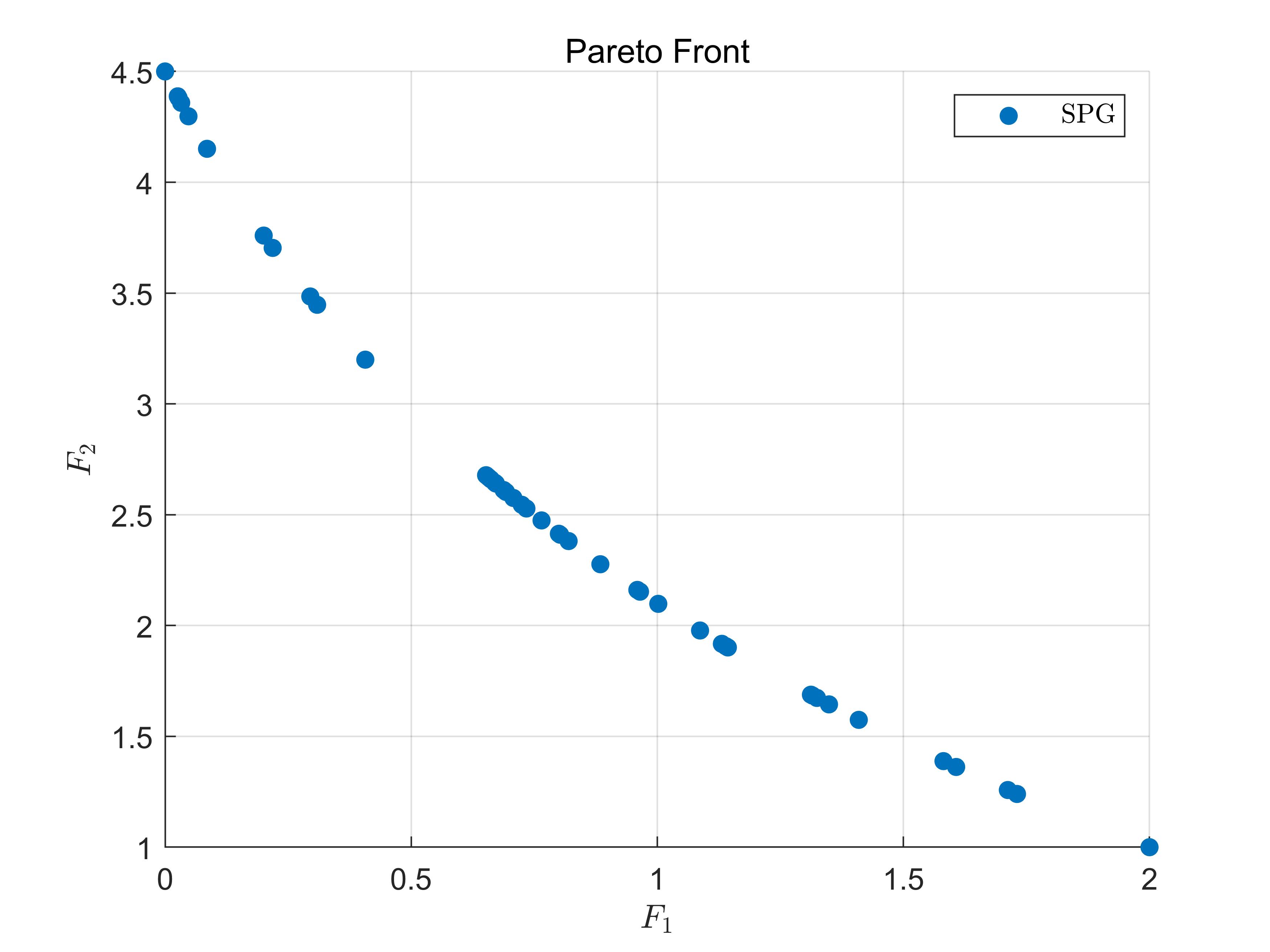
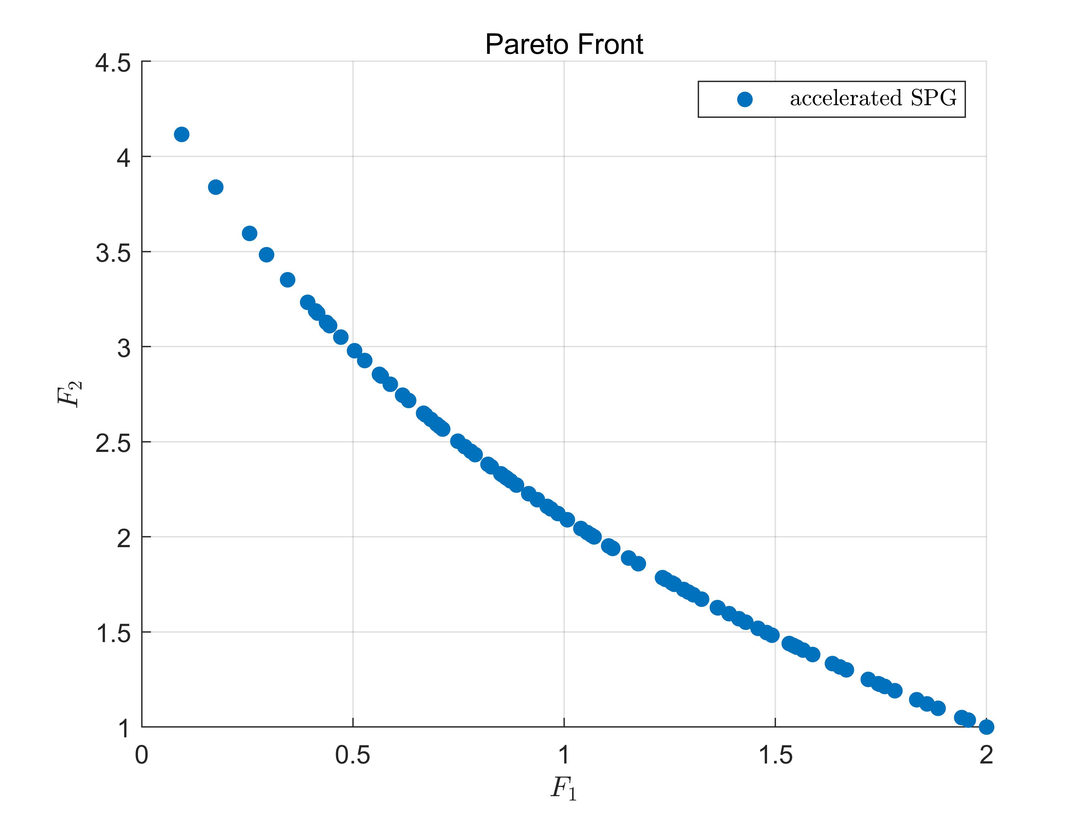
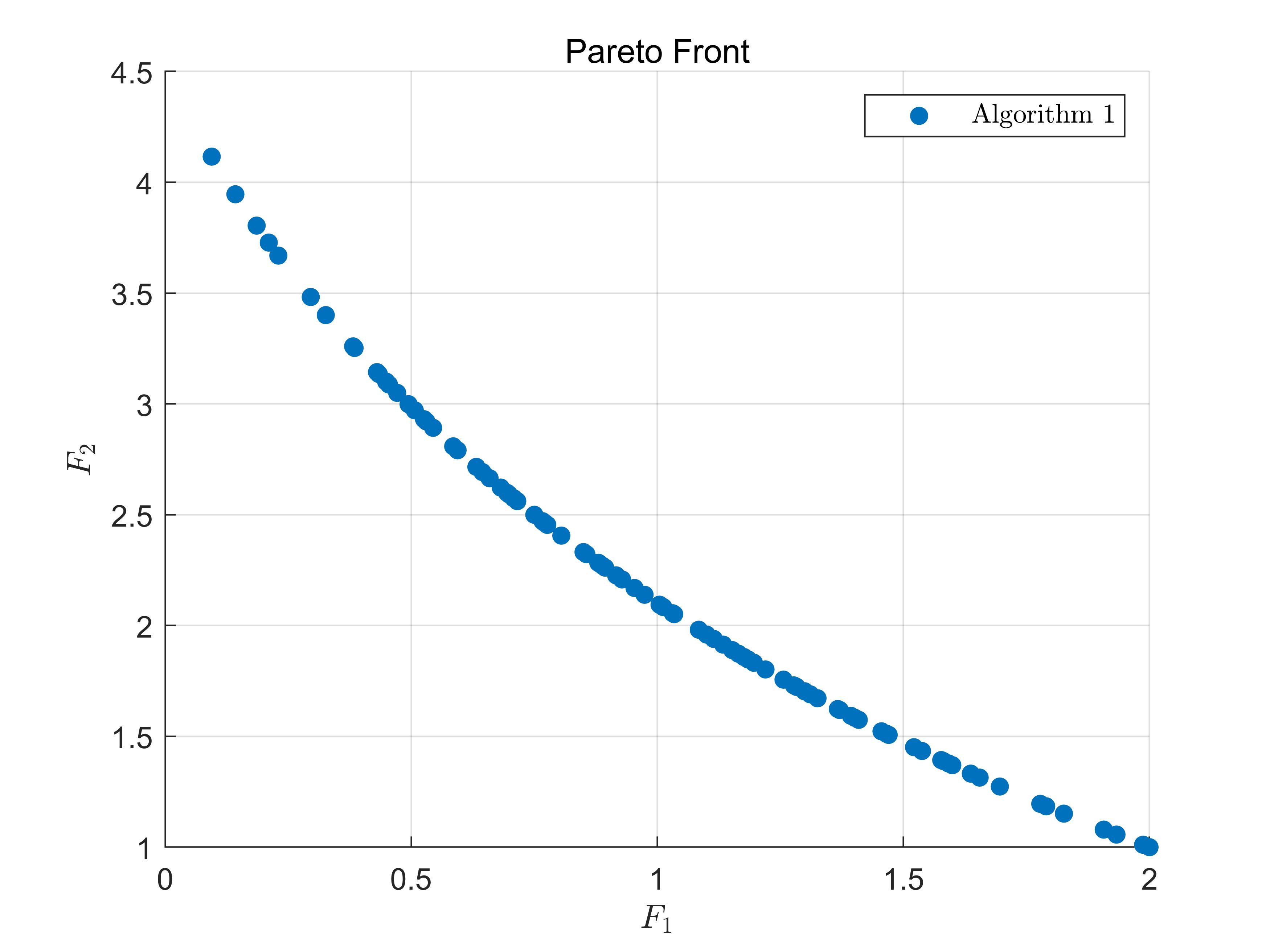
Figure 1: The final Pareto front for JOS1 with $n=50$.

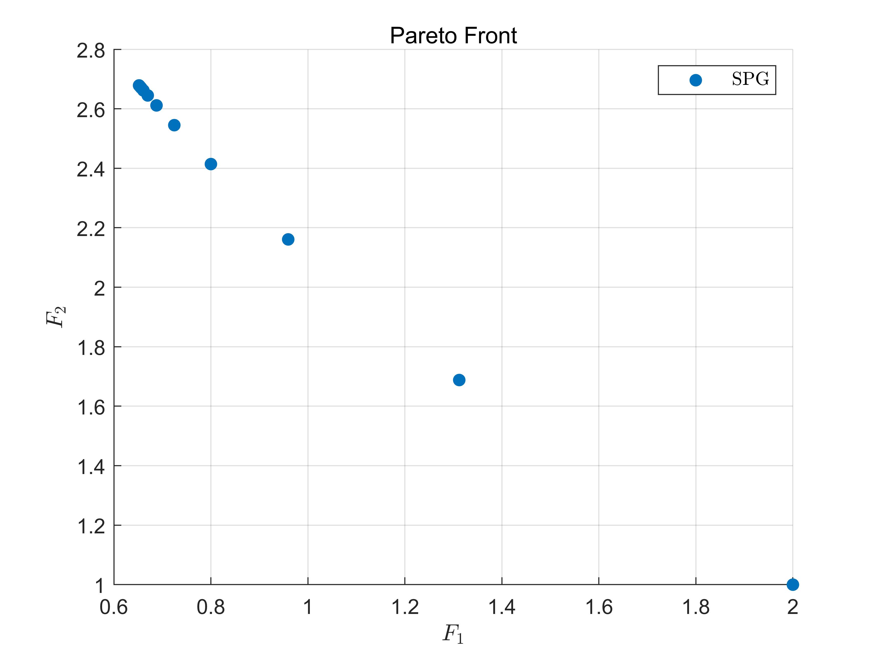
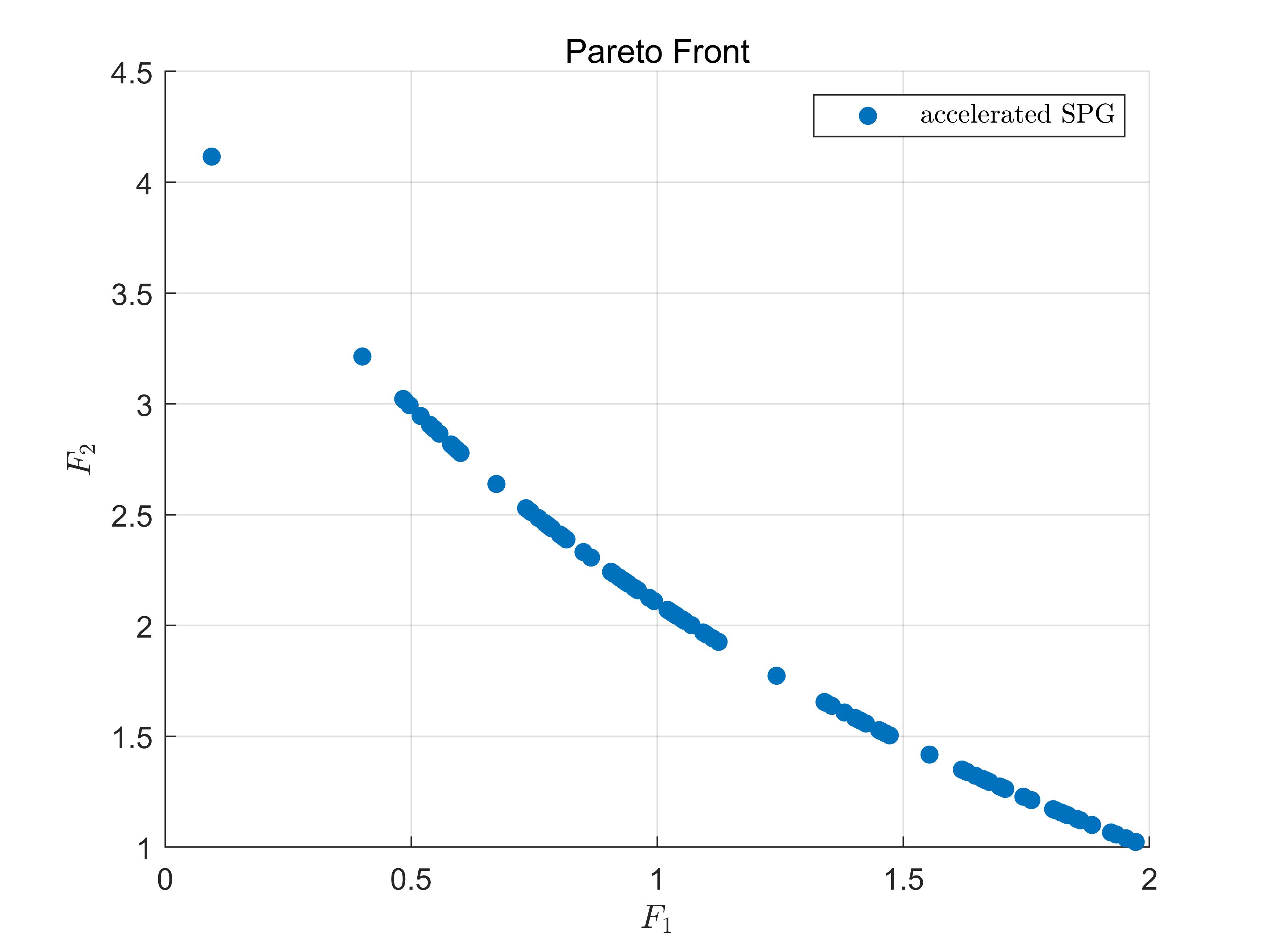
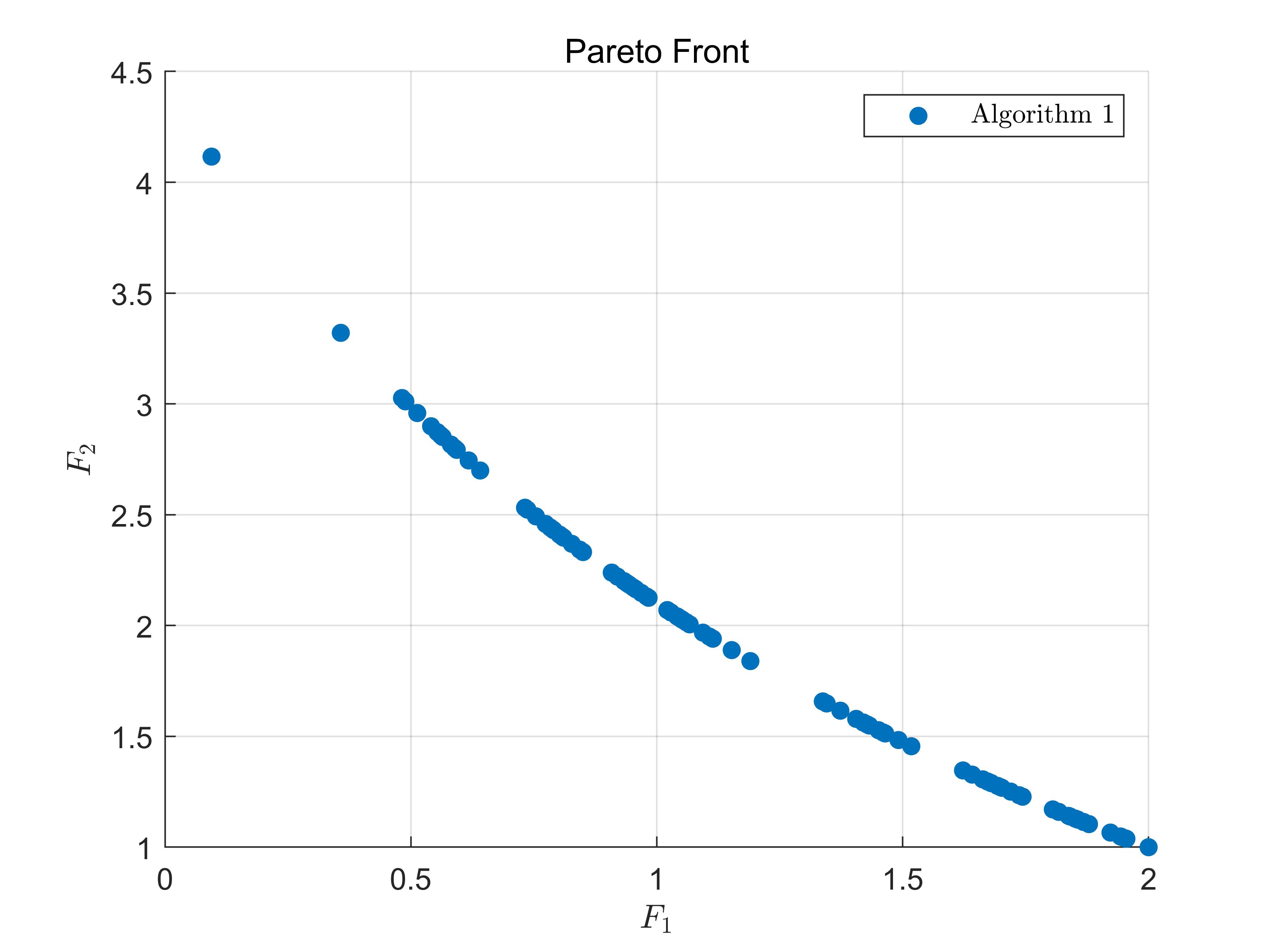
Figure 2: The final Pareto front for JOS1 with $n=500$.

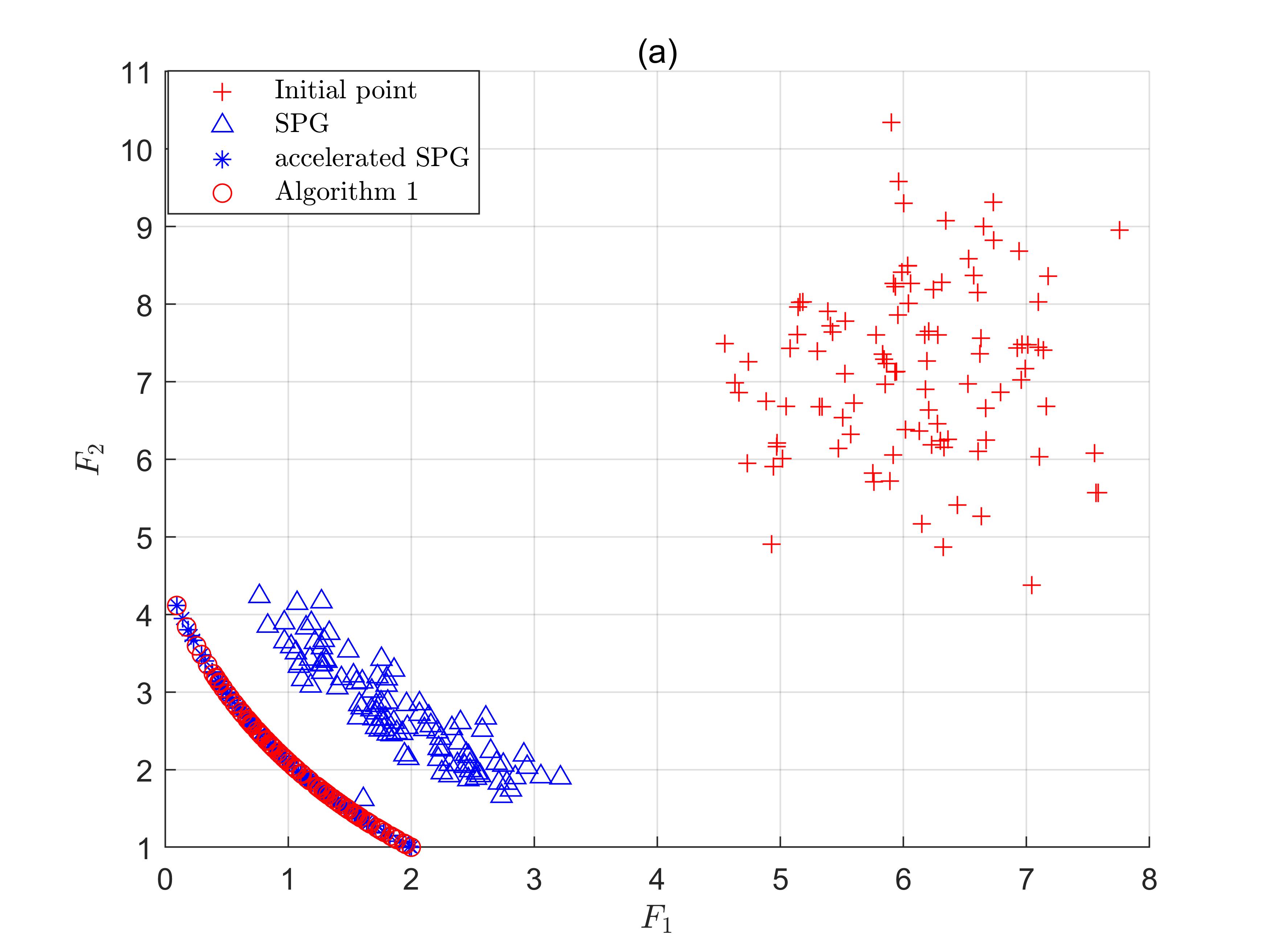
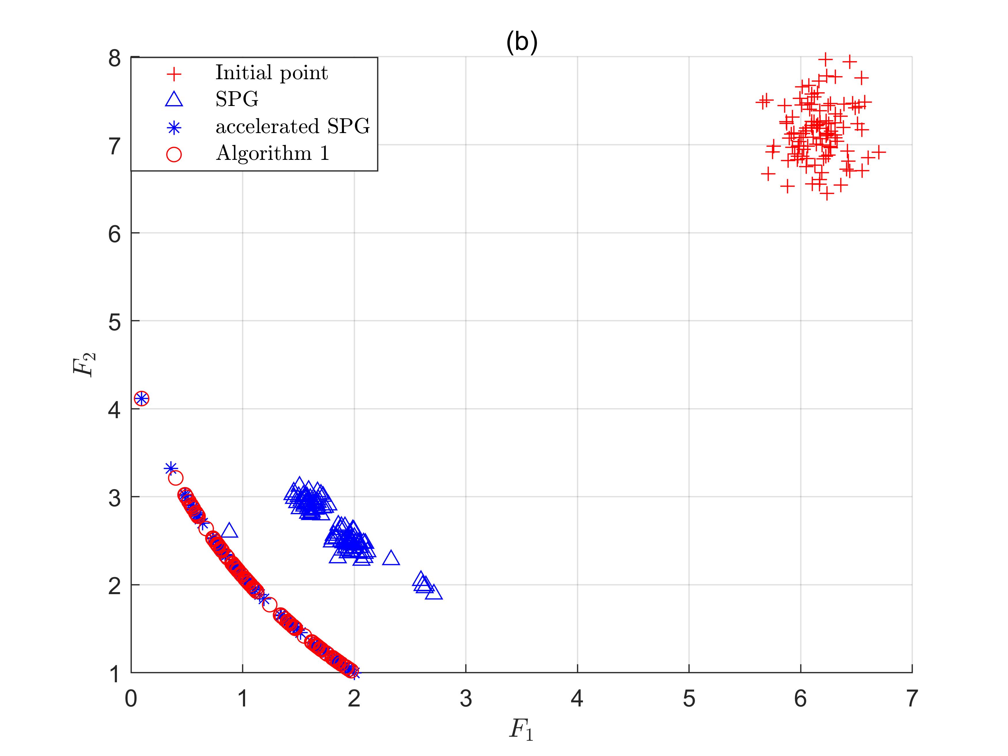
Figure 3: The comparison results of Pareto front for JOS1 with $n=50$ (left) and $n=500$ (right) when $k=2$.

Table 2:

Problem	$n$	$g_{i}$	Averge time($\times 0.01$)			Averge iteration counts
			SPG	accelerated SPG	Algorithm 1	SPG	accelerated SPG	Algorithm 1
JOS1	5	0	0.080	0.070	0.070	2	2	2
JOS1	5	$l_{1}$	0.800	0.130	0.120	20.91	2	2
JOS1	50	0	0.120	0.110	0.090	3	2	2
JOS1	50	$l_{1}$	1.050	0.150	0.140	22.87	2	2
JOS1	500	0	0.150	0.140	0.130	3	2	2
JOS1	500	$l_{1}$	1.200	0.250	0.220	27.08	2	2
JOS1	1000	0	0.230	0.190	0.190	3	2	2
JOS1	1000	$l_{1}$	1.330	0.280	0.280	25.48	2	2
SD	4	ind	10.610	6.950	5.870	885.1	827.98	777.89
TOI	4	0	0.860	0.100	0.090	1382.14	35.47	32.36
TOI	4	$l_{1}$	4.940	0.430	0.380	46.93	21.45	22.06
TRIDIA	3	0	1.520	1.440	1.250	1781.86	714.53	713.46
TRIDIA	3	$l_{1}$	2.800	1.850	1.730	171.55	115.66	90.2
FDS	5	0	1.120	0.720	0.630	151.25	148.74	132.05
FDS	5	$l_{1}$	166.560	129.250	121.580	668.04	1037.4	1005.38
FDS	50	0	5.010	3.070	2.800	370.24	343.09	316.12
FDS	50	$l_{1}$	490.460	390.130	365.410	1361.48	2001	2001.000
FDS	100	0	6.560	4.370	3.900	432.18	379.16	348.97
FDS	100	$l_{1}$	539.420	407.550	356.840	1923.67	2001	2001

7 Conclusions

In this paper, we introduce a fast proximal gradient algorithm for multiobjective optimization (denoted as Algorithm 1). We demonstrate that the convergence rate of the accelerated algorithm for multiobjective optimization developed by Tanabe et al. can be enhanced from $O(1/k^{2})$ to $o(1/k^{2})$ by incorporating a distinct extrapolation term $\frac{k-1}{k+\alpha-1}$ with $\alpha>3$. Furthermore, we establish an inexact version of the Algorithm 1 when the condition of summable error terms is met, and the convergence rate matches that of the Algorithm 1. This resolves the open issues raised in this article Sonntag1 . Finally, we validate the efficiency of the proposed algorithm through some examples.

References

• [1] Ansary, M. A. T. A newton-type proximal gradient method for nonlinear multi-objective optimization problems. Optimization Methods and Software, 38:570-590, 2023.
• [2] Attouch, H., Peypouquet, J.: The rate of convergence of Nesterovs accelerated forward-backward method is actually faster than $o(1/k^{2})$. SIAM J. Optim. 26(3), 1824-1834 (2016)
• [3] Attouch, H., Chbani, Z., Peypouquet, J., Redont, P.: Fast convergence of inertial dynamics and algorithms with asymptotic vanishing viscosity. Math. Program. 168(1-2), 123-175 (2018)
• [4] Beck, A.: First-Order Methods in Optimization, Society for Industrial and Applied Mathematics, 2017.
• [5] Carrizo, G. A., Lotito, P. A., Maciel, M. C. (2016). Trust region globalization strategy for the nonconvex unconstrained multiobjective optimization problem. Mathematical Programming, 159, 339-369.
• [6] Chambolle, A., Dossal, C.: On the convergence of the iterates of the ”fast iterative shrinkage/thresholding algorithm” . J. Optim. Theory Appl. 166, 968-982 (2015)
• [7] Chen J, Tang L, Yang X. A Barzilai-Borwein descent method for multiobjective optimization problems. European Journal of Operational Research, 311(1):196-209, 2023.
• [8] Chen W, Yang X, Zhao Y. Conditional gradient method for vector optimization[J]. Computational Optimization and Applications, 2023: 1-40.
• [9] Boyd, S., Vandenberghe, L.: Introduction to applied linear algebra: vectors, matrices, and least squares. Cambridge university press (2018).
• [10] Fliege, J., Svaiter, B. F. (2000). Steepest descent methods for multicriteria optimization. Mathematical Methods of Operations Research, 51, 479-494.
• [11] Fliege, J., Drummond, L. M., Svaiter, B. F. (2009). Newton’s method for multiobjective optimization. SIAM Journal on Optimization,20, 602-626.
• [12] Fukuda E H, Drummond L M G. A survey on multiobjective descent methods[J]. Pesquisa Operacional, 2014, 34: 585-620.
• [13] Lucambio Perez, L. R., Prudente, L. F. (2018). Nonlinear conjugate gradient methods for vector optimization. SIAM Journal on Optimization, 28, 2690-2720.
• [14] Tanabe, H., Fukuda, E. H. and Yamashita, N.: New merit functions and error bounds for non-convex multiobjective optimization, arXiv: 2010.09333, 2020.
• [15] Tanabe H, Fukuda E H, Yamashita N. An accelerated proximal gradient method for multiobjective optimization[J]. Computational Optimization and Applications, 2023: 1-35.
• [16] H. Tanabe, E. H. Fukuda, and N. Yamashita. Proximal gradient methods for multiobjective optimization and their applications. Computational Optimization and Applications, 72(2):339-361, 2019.
• [17] Tanabe H, Fukuda E H, Yamashita N. A globally convergent fast iterative shrinkage-thresholding algorithm with a new momentum factor for single and multi-objective convex optimization[J]. arXiv preprint arXiv:2205.05262, 2022.
• [18] Mita, K., Fukuda, E.H., Yamashita, N.: Nonmonotone line searches for unconstrained multiobjective optimization problems. J. Global Optim. 75,63-90 (2019)
• [19] Nishimura, Yuki, Ellen H. Fukuda, and Nobuo Yamashita. ”Monotonicity for Multiobjective Accelerated Proximal Gradient Methods.” arXiv preprint arXiv:2206.04412 (2022).
• [20] Opial, Z. (1967). Weak convergence of the sequence of successive approximations for nonexpansive mappings.
• [21] Sonntag K, Peitz S. Fast Multiobjective Gradient Methods with Nesterov Acceleration via Inertial Gradient-like Systems[J]. arXiv preprint arXiv:2207.12707, 2022.
• [22] Sonntag K, Peitz S. Fast convergence of inertial multiobjective gradient-like systems with asymptotic vanishing damping[J]. arXiv preprint arXiv:2307.00975, 2023.