Misalignment production of vector boson dark matter from axion-SU(2) inflation

Abstract

We present a new mechanism to generate a coherently oscillating dark vector field from axion-SU(2) gauge field dynamics during inflation. The SU(2) gauge field acquires a nonzero background sourced by an axion during inflation, and it acquires a mass through spontaneous symmetry breaking after inflation. We find that the coherent oscillation of the dark vector field can account for dark matter in the mass range of $10^{-13}\,\text{--}\,1$ eV in a minimal setup. In a more involved scenario, the range can be wider down to the fuzzy dark matter region. One of the dark vector fields can be identified as the dark photon, in which case this mechanism evades the notorious constraints for isocurvature perturbation, statistical anisotropy, and the absence of ghosts that exist in the usual misalignment production scenarios. Phenomenological implications are discussed.

I Introduction

The existence of dark matter is well established by astronomical and cosmological observations. However, the nature of dark matter remains unknown, and various candidates have been proposed in the literature. One of the candidates is a dark photon, which is a gauge boson associated with a hidden U(1) gauge symmetry. There are various known scenarios to produce dark photon particles or excitations as dark matter: gravitational production Graham:2015rva ; Ema:2019yrd ; Ahmed:2020fhc ; Kolb:2020fwh ; Li:2021fao ; Sato:2022jya ; Redi:2022zkt , gravitational thermal scattering Tang:2017hvq ; Garny:2017kha , production through axion-like couplings Agrawal:2018vin ; Co:2018lka ; Bastero-Gil:2018uel ; Moroi:2020has , Higgs dynamics Dror:2018pdh ; Nakayama:2021avl , kinetic couplings Salehian:2020asa ; Firouzjahi:2020whk ; Nakai:2022dni ; Adshead:2023qiw , thermal production with the bose-enhancement effect Yin:2023jjj , and cosmic strings Long:2019lwl ; Kitajima:2022lre . Moreover, a coherent oscillation of a dark photon field can also account for dark matter.

Initially, a minimal setup for misalignment production of dark photon dark matter was originally proposed in Ref. Nelson:2011sf , which does not work due to the Hubble mass term for the canonically normalized gauge field. To cancel out this Hubble mass term, an introduction of a non-minimal coupling of dark photons to gravity was proposed Arias:2012az , although it is also excluded by the existence of ghost modes Nakayama:2019rhg . Currently, one of the viable scenarios for the generation of a coherent dark photon dark matter is that proposed in Ref. Kitajima:2023fun . This scenario is based on the model where the inflaton $\phi$ coupled with the dark photon through the kinetic function as $f^{2}(\phi)F_{\mu\nu}F^{\mu\nu}$ Nakayama:2019rhg . To avoid the observational constraints pointed out in Ref. Nakayama:2020rka , they introduced a curvaton field to the model in Ref. Nakayama:2019rhg .

In Ref. Nakayama:2020rka , the original model is ruled out due to the combination of the statistical anisotropy of the curvature perturbations and the isocurvature perturbations. The former arises because the coherent U(1) gauge field determines one specific direction. In this regard, an SU(2) gauge field can take an isotropic configuration thanks to its three gauge degrees of freedom. Actually, such a configuration is dynamically realized in an inflationary model called chromo-natural inflation Adshead:2012kp , where the inflaton is coupled to the SU(2) gauge field through a topological coupling, $\phi F_{\mu\nu}^{a}\tilde{F}^{a\mu\nu}$, and the inflaton velocity assists the isotropic configuration of the SU(2) gauge field (see Ref. Komatsu:2022nvu for a recent review). Although the original chromo-natural inflation model with a cosine-type potential is excluded due to a significant production of gravitational waves Dimastrogiovanni:2012ew ; Adshead:2013qp ; Adshead:2013nka , this constraint can be evaded by considering a modification of the axion potential Caldwell:2017chz . In fact, such a gravitational waves production is suppressed with a low inflation scale Komatsu:2022nvu , which will be our focus (see low scale axion inflation models, such as the multi-natural inflation Czerny:2014wza ; Czerny:2014xja ; Czerny:2014qqa ; Higaki:2014sja , ALP inflation Daido:2017wwb ; Daido:2017tbr ; Takahashi:2019qmh ; Takahashi:2021tff ; Takahashi:2023vhv , hybrid QCD axion inflation Narita:2023naj , and the UV completions Czerny:2014xja ; Czerny:2014qqa ; Higaki:2014sja ; Murai:2023gkv ; Croon:2014dma ; Higaki:2015kta ; Higaki:2016ydn ). In this case, the scenario is free from the constraint of isocurvature perturbations Adshead:2013nka ; Adshead:2016omu .

In this paper, we use this mechanism to generate coherent vector dark matter while avoiding the constraints from the curvature and isocurvature perturbations. Our scenario includes two important stages: the dynamics of an axion and SU(2) gauge field during inflation and the oscillation of a homogeneous gauge field after inflation. During inflation, an axion drives inflation and sources the homogeneous mode of an SU(2) gauge field through the topological coupling. After inflation, the axion decays into standard model particles and stops to source the SU(2) gauge field. Then, the SU(2) gauge field independently oscillates due to its self-coupling term. Whether the SU(2) gauge symmetry is spontaneously broken as the cosmic temperature decreases or initially broken during inflation, the SU(2) gauge field background is inherited by a massive gauge field in the late time universe. The field starts to oscillate due to its mass and behaves as non-relativistic matter. Then, the massive gauge field can account for dark matter. Finally, giving a higher dimensional mixing term with standard model photon, we show that the mechanism is consistent for the misalignment production of the dark photon dark matter by taking account of the observational and experimental constraints. We also discuss the phenomenological implications such as dark matter search and dark radiation prediction.

The rest of this paper is organized as follows. In Sec. II, we discuss the dynamics of the axion and SU(2) gauge field and the homogeneous configuration of the SU(2) gauge field during inflation. In Sec. III, we investigate the evolution of the gauge field after inflation and evaluate the abundance of the coherently oscillating vector dark matter. As a realization of the mechanism, we study a model in which the SSB is induced by an SU(2) doublet vacuum expectation value. In Sec. IV, we introduce the mixing term to photon and show that it can apply to the misalignment production of the dark photon dark matter. Sec. V is devoted to the summary and discussion of our results.

II Generation of homogeneous SU(2) gauge field during inflation

First, we focus on the dynamics during inflation. The relevant terms of the Lagrangian are given by

$$\mathcal{L}_{\mathrm{inf}}=\frac{1}{2}\partial_{\mu}\phi\partial^{\mu}\phi-V(\phi)-\frac{1}{4}F_{\mu\nu}^{a}F^{a\mu\nu}+\frac{1}{4f}\phi F_{\mu\nu}^{a}\tilde{F}^{a\mu\nu}\ ,$$ (1)

where $V(\phi)$ is the potential of the axion field $\phi$, and $f$ controls the strength of the topological coupling. Although our discussion also works for $\phi$ being a spectator field as in Ref. Dimastrogiovanni:2016fuu , we consider that $\phi$ is the inflaton as the minimal scenario. In the following, we do not specify the form of $V(\phi)$. The field strength and its dual of the SU(2) gauge field are defined by

$$F_{\mu\nu}^{a} \equiv\partial_{\mu}A_{\nu}^{a}-\partial_{\nu}A_{\mu}^{a}-g\epsilon^{abc}A_{\mu}^{b}A_{\nu}^{c}\ ,$$ (2)

$$\tilde{F}^{a\mu\nu} \equiv\frac{\epsilon^{\mu\nu\rho\sigma}}{2\sqrt{-\det[g_{\mu\nu}]}}F_{\rho\sigma}^{a}\ ,$$ (3)

where $A_{\mu}^{a}$ is the SU(2) gauge field, $g$ is the SU(2) gauge coupling, $g_{\mu\nu}$ is the space-time metric, and $\epsilon^{abc}$ and $\epsilon^{\mu\nu\rho\sigma}$ are totally anti-symmetric tensors. Here, we neglect the vector field mass. This is justified if the Hubble parameter (Eq. (6)) during inflation is much higher than the gauge boson mass. As we will see in the next section, this condition is always satisfied by requiring the correct dark matter abundance even if the SU(2) is spontaneously broken before inflation.

In the following, we adopt the temporal gauge, $A_{0}^{a}=0$, and focus on homogeneous modes of the axion and gauge fields:

$$\phi(t,\bm{x})=\phi(t)\ ,\quad A_{i}^{a}(t,\bm{x})=A_{i}^{a}(t)\ .$$ (4)

We also assume the flat FLRW metric for the space-time metric,

$$\mathrm{d}s^{2}=g_{\mu\nu}\mathrm{d}x^{\mu}\mathrm{d}x^{\nu}=\mathrm{d}t^{2}-a(t)^{2}(\mathrm{d}x^{2}+\mathrm{d}y^{2}+\mathrm{d}z^{2})\ .$$ (5)

The time evolution of the scale factor, $a(t)$, is governed by the Friedmann equation,

$$H^{2}\equiv\left(\frac{\dot{a}}{a}\right)^{2}=\frac{\rho_{\phi}+\rho_{A}}{3M_{\mathrm{Pl}}^{2}}\ ,$$ (6)

where the dot represents a derivative with respect to $t$, $M_{\mathrm{Pl}}\simeq 2.4\times 10^{18}$ GeV is the reduced Planck mass, and the energy densities of the inflaton and gauge field are given by

$$\rho_{\phi} =\frac{1}{2}\dot{\phi}^{2}+V(\phi)\ ,$$ (7)

$$\rho_{A} =\frac{1}{2a^{2}}\dot{A}_{i}^{a}\dot{A}_{i}^{a}+\frac{g^{2}}{4a^{4}}\left[\left(A_{i}^{a}A_{i}^{a}\right)^{2}-A_{i}^{a}A_{i}^{b}A_{j}^{a}A_{j}^{b}\right]\ ,$$ (8)

respectively.

The equations of motion for the homogeneous fields are given by

$$\ddot{\phi}+3H\dot{\phi}+\frac{\partial V}{\partial\phi} =-\frac{g}{2fa^{3}}\epsilon^{ijk}\epsilon^{abc}\dot{A}_{i}^{a}A_{j}^{b}A_{k}^{c}\ ,$$ (9)

$$\ddot{A}_{i}^{a}+H\dot{A}_{i}^{a}+\frac{g^{2}}{a^{2}}\left(A_{j}^{b}A_{j}^{b}A_{i}^{a}-A_{j}^{a}A_{i}^{b}A_{j}^{b}\right) =\frac{g}{2fa}\dot{\phi}\epsilon^{ijk}\epsilon^{abc}A_{j}^{b}A_{k}^{c}\ .$$ (10)

From the equation of motion for the gauge field, we expect that the axion velocity can source the gauge field. If the axion field rolls down the potential fast enough, it is known that the homogeneous gauge field has an isotropic attractor solution Adshead:2012kp ; Maleknejad:2013npa ; Wolfson:2020fqz ; Wolfson:2021fya , which has the form of

$$A_{i}^{a}=\delta_{i}^{a}a(t)Q(t)\ .$$ (11)

We substitute this ansatz into the equations of motion and obtain

$$\ddot{\phi}+3H\dot{\phi}+\frac{\partial V}{\partial\phi} =-\frac{3g}{f}Q^{2}\left(\dot{Q}+HQ\right)\ ,$$ (12)

$$\ddot{Q}+3H\dot{Q}+\left(\dot{H}+2H^{2}\right)Q+2g^{2}Q^{3} =\frac{g}{f}Q^{2}\dot{\phi}\ .$$ (13)

The energy density of the gauge field, Eq. (8), is also simplified as

$$\rho_{A}=\frac{3}{2}\left(\dot{Q}+HQ\right)^{2}+\frac{3}{2}g^{2}Q^{4}\ .$$ (14)

Here, we approximate that the Hubble parameter is constant and focus on the stationary solution, $\ddot{Q},H\dot{Q}\ll H^{2}Q$ and $\ddot{\phi}\ll H\dot{\phi}$, with which the energy density $\rho_{A}$ is also approximately constant. Note that we keep $\dot{\phi}$ because the motion of $\phi$ is important in that it sources the gauge field. Then, we simplify the equations of motion as

$$3H\dot{\phi}+\frac{\partial V}{\partial\phi} =-\frac{3g}{f}HQ^{3}\ ,$$ (15)

$$2H^{2}Q+2g^{2}Q^{3} =\frac{g}{f}Q^{2}\dot{\phi}\ .$$ (16)

It is convenient to introduce dimensionless parameters that characterize the amplitude of the gauge field, the velocity of the axion field, and the strength of the $\phi F\tilde{F}$ coupling by

$$m_{Q}\equiv\frac{gQ}{H}\ ,\quad\xi\equiv\frac{\dot{\phi}}{2fH}\ ,\quad\Lambda_{Q}\equiv\frac{Q}{f}\ ,$$ (17)

respectively. Obviously, the equations of motion have a trivial solution,

$$Q=0\ ,\quad\dot{\phi}=-\frac{1}{3H}\frac{\partial V}{\partial\phi}\ .$$ (18)

There is also a nontrivial solution with $Q\neq 0$. In the case of $\Lambda_{Q}\gg 1$, the backreaction from the gauge field in the right-hand side of Eq. (15) becomes much larger than the Hubble friction term. Then, we obtain

$$m_{Q}=\left(-\frac{g^{2}f}{3H^{4}}\frac{\partial V}{\partial\phi}\right)^{1/3}\ ,$$ (19)

$$m_{Q}^{3}-\xi m_{Q}^{2}+m_{Q}=0\ ,$$ (20)

which leads to

$$m_{Q}=0,\frac{\xi\pm\sqrt{\xi^{2}-4}}{2}\ .$$ (21)

To see which solution realizes, we define the effective potential for $m_{Q}$ by integrating the left-hand side of Eq. (20) with respect to $m_{Q}$ as

$$V_{\mathrm{eff}}(m_{Q})\equiv\frac{1}{4}m_{Q}^{4}-\frac{\xi}{3}m_{Q}^{3}+\frac{1}{2}m_{Q}^{2}\ .$$ (22)

We show the shape of the effective potential in Fig. 1. Regardless of the value of $\xi$, this potential has a local minimum at $m_{Q}=0$. In addition, it has another minimum at $m_{Q}=(\xi+\sqrt{\xi^{2}-4})/2$ for $\xi>2$, which becomes the global minimum for $\xi>\xi_{\mathrm{c}}\equiv 3/\sqrt{2}\simeq 2.12$. Note that the other solution of Eq. (20), $m_{Q}=(\xi-\sqrt{\xi^{2}-4})/2$, corresponds to the local maximum of $V_{\mathrm{eff}}$ for $\xi>2$. Thus, we expect that the nontrivial solution is realized for $\xi\gtrsim\xi_{\mathrm{c}}$.

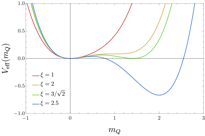
Figure 1: Effective potential for $\xi$ = $1$, $2$, $3/\sqrt{2}$, $2.5$. The potential has a local minimum at $m_{Q}\neq 0$ for $\xi>2$, and it becomes the global minimum for $\xi>3/\sqrt{2}$.

When the gradient of the axion potential becomes large enough, the slow-roll condition is violated and inflation ends. The slow-roll parameter is given by

$$\epsilon_{H}\equiv-\frac{\dot{H}}{H^{2}}=\epsilon_{\phi}+\epsilon_{E}+\epsilon_{B}\ ,$$ (23)

where

$$\epsilon_{\phi}\equiv\frac{\dot{\phi}^{2}}{2M_{\mathrm{Pl}}^{2}H^{2}}\ ,\quad\epsilon_{E}\equiv\frac{\left(\dot{Q}+HQ\right)^{2}}{M_{\mathrm{Pl}}^{2}H^{2}}\ ,\quad\epsilon_{B}\equiv\frac{g^{2}Q^{4}}{M_{\mathrm{Pl}}^{2}H^{2}}\ .$$ (24)

With the stationary solution, in particular, the slow-roll parameters are given by

$$\epsilon_{\phi}=\frac{2\xi^{2}f^{2}}{M_{\mathrm{Pl}}^{2}}\ ,\quad\epsilon_{E}=\frac{m_{Q}^{2}H^{2}}{g^{2}M_{\mathrm{Pl}}^{2}}\ ,\quad\epsilon_{B}=\frac{m_{Q}^{4}H^{2}}{g^{2}M_{\mathrm{Pl}}^{2}}\ .$$ (25)

For $\Lambda_{Q}\gg 1$, we obtain

$$\frac{\epsilon_{B}}{\epsilon_{\phi}}=\frac{m_{Q}^{2}\Lambda_{Q}^{2}}{2\xi^{2}}\gg 1\ ,$$ (26)

and thus $\epsilon_{B}$ is dominant in the total slow-roll parameter $\epsilon_{H}$. Thus, we define the end of inflation by $\epsilon_{B}=1$ in the following.

III Vector dark matter from axion-SU(2) inflation

In this section, we study the evolution of vector dark matter in our mechanism by using a concrete example.

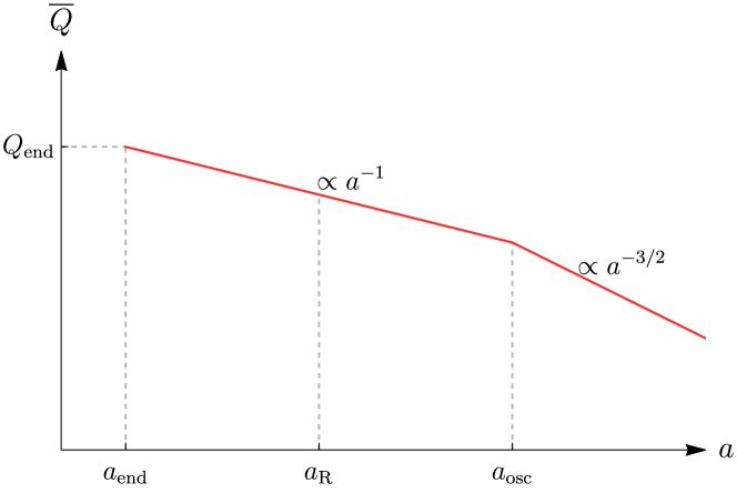
Figure 2: Time evolution of the amplitude of the gauge field, $\overline{Q}$ in the pre-inflationary scenario. At the end of inflation, the SU(2) gauge field has a nonzero background, $Q_{\mathrm{end}}$, due to the axion-gauge field dynamics during inflation. Then, the gauge field starts to oscillate due to the quartic potential of $Q$ originating from the self-coupling and $\overline{Q}$ decreases as $\propto a^{-1}$. Once the mass potential induced by the SSB overcomes the quartic potential, the gauge field comes to behave as non-relativistic matter with $\overline{Q}\propto a^{-3/2}$.

We consider the simplest scenario with an SU(2) doublet, $\Phi$, to give mass to the gauge fields. The relevant Lagrangian is given by

$$\mathcal{L}_{\mathrm{SSB}}=D_{\mu}\Phi^{\dagger}D^{\mu}\Phi-V_{\mathrm{d}}(\Phi)\ ,$$ (27)

where the covariant derivative, $D_{\mu}$, is defined by

$$D_{\mu}\Phi=\partial_{\mu}\Phi-igA_{\mu}^{a}\frac{\sigma^{a}}{2}\Phi\ .$$ (28)

Here, $\sigma^{a}$ is the Pauli matrix, and the potential is assumed to be

$$V_{\mathrm{d}}(\Phi)=\frac{\lambda}{4}\left(\Phi^{\dagger}\Phi-v^{2}\right)^{2}\ ,$$ (29)

with a positive constant $\lambda$. Considering that this potential has a negative mass term, $-\lambda v^{2}\Phi^{\dagger}\Phi/2$, $\Phi$ is expected to acquire a nonzero expectation value either before or after inflation.

Once the SU(2) symmetry is spontaneously broken, the gauge field acquires a mass term given by

$$\mathcal{L}\supset\frac{g^{2}v^{2}}{4}A_{\mu}^{a}A^{a\mu}\ ,$$ (30)

which corresponds to a mass of $m=gv/\sqrt{2}$. In this case, the three components of the SU(2) gauge field become massive at the SSB. The masses are the same. This is a specific spectrum with the single double Higgs field breaking the SU(2).

In the following, we will discuss the scenario with the SSB before inflation (pre-inflationary scenario) and after inflation (post-inflationary scenario). In Fig. 2, we summarize the time evolution of the amplitude of the oscillating gauge field, $\overline{Q}$ in the pre-inflationary scenario.

III.1 Pre-inflationary scenario and abundance of the massive vector fields

Let us first consider the possibility that the SU(2) is always broken during and after inflation. This is the case if the Higgs boson mass satisfies

$$m_{\Phi}\gg H\ ,$$ (31)

during inflation, and the matter effect never lets the symmetry recover. Here $m_{\Phi}\simeq\sqrt{\lambda}v$ at the tree-level. Although the gauge fields contribute to the effective mass of the Higgs field, it is of the order of $gQ=m_{Q}H$ and is not important due to the condition (31). Again, we consider that the gauge boson mass satisfies $m\ll H$ around the end of inflation. This will be shown to be a self-consistent condition in the following.

We also emphasize that the discussion in this section is within an effective theory and it is not sensitive to UV completion other than the mass spectrum of the three vector bosons. After inflation, the inflaton typically starts to oscillate around its potential minimum, and the gauge field deviates from the static solution given by Eq. (19).

Although the evolution of the axion and gauge field depends on the detail of reheating, we can expect that the axion rapidly loses its energy density and the gauge field starts to evolve independently soon after the end of inflation (for instance, see the model in Ref. Moroi:2020has ).

First, we evaluate the amplitude of the gauge field at the end of inflation. From the condition of $\epsilon_{B}=1$, we obtain the gauge field amplitude at the end of inflation as

$$m_{Q,\mathrm{end}}=\frac{gQ_{\mathrm{end}}}{H_{\mathrm{end}}}\simeq\sqrt{\frac{gM_{\mathrm{Pl}}}{H_{\mathrm{end}}}}\ ,$$ (32)

where the subscript “end” denotes quantities at the end of inflation. Note that this relation leads to $Q_{\mathrm{end}}=M_{\mathrm{Pl}}/m_{Q,\mathrm{end}}$, and the gauge field amplitude is smaller than the Planck scale by $m_{Q,\mathrm{end}}$. To satisfy $\Lambda_{Q}=Q/f\gg 1$ at the end of inflation, we require $f\ll M_{\mathrm{Pl}}$ in the following. Similarly, we will use the subscripts “R”, “SSB”, and “osc” for quantities at the completion of reheating, the SSB of SU(2) (in the next subsection), and the onset of gauge field oscillations due to the mass, respectively. While the nontrivial solution exists for $m_{Q}\geq 1$, the backreaction from the enhanced perturbations becomes non-negligible for large $m_{Q}$ depending on the value of $g$ Fujita:2017jwq ; Ishiwata:2021yne . The requirement becomes $m_{Q}\lesssim O(10)$ for $g=10^{-O(10)}$, which we will focus on in the following. In the following, we will treat $m_{Q,\mathrm{end}}$ as a fixed parameter, which relates $H_{\mathrm{end}}$ and $g$ as

$$H_{\mathrm{end}}=\frac{gM_{\mathrm{Pl}}}{m_{Q,\mathrm{end}}^{2}}\ .$$ (33)

Even after inflation, there is no reason for the gauge field to deviate from the isotropic configuration in Eq. (11). Thus, we follow the evolution of $Q$ in the following. Once the gauge field decouples from the axion, the equation of motion for $Q$ becomes

$$\ddot{Q}+3H\dot{Q}+\left(\dot{H}+2H^{2}+m^{2}\right)Q+2g^{2}Q^{3} =0\ .$$ (34)

Until the completion of reheating, the universe is dominated by the oscillating inflaton, which is assumed to behave as non-relativistic matter as usual. Thus, $H=2/(3t)$ and we obtain

$$\ddot{Q}+3H\dot{Q}+\left(\frac{H^{2}}{2}+m^{2}\right)Q+2g^{2}Q^{3} =0\ .$$ (35)

This EoM can be understood as that for a scalar field with the mass including the Hubble-induced term and the quartic potential. Just after inflation, $m_{Q,\mathrm{end}}>1$, and the dynamics of the gauge field is controlled by the quartic potential since $m$ is smaller than $H_{\mathrm{end}}$. Then, $Q$ oscillates with a decreasing amplitude of $\overline{Q}\propto a^{-1}$. Since $H$ decreases as $\propto t^{-1}\propto a^{-3/2}$, $m_{Q}$ remains larger than unity even after inflation. Thus, we consider that the amplitude of $Q$ decreases as $a^{-1}$ until the completion of reheating.

The completion of reheating is represented by

$$\Gamma_{\phi}=H=\sqrt{\frac{\pi^{2}g_{*,\mathrm{R}}}{90}}\frac{T_{\mathrm{R}}^{2}}{M_{\mathrm{Pl}}}\ ,$$ (36)

where $\Gamma_{\phi}$ is the decay width of the inflaton, $T_{\mathrm{R}}$ is the reheating temperature, and $g_{*}$ is the relativistic degrees of freedom for the energy density. Since the Hubble parameter evolves as $H\propto a^{-3/2}$ during reheating, the ratio of the scale factors between the end of inflation and the completion of reheating becomes

$$c\equiv\frac{a_{\mathrm{R}}}{a_{\mathrm{end}}}=\left(\frac{H_{\mathrm{end}}}{\Gamma_{\phi}}\right)^{2/3}\ .$$ (37)

With the factor $c\geq 1$, the reheating temperature is represented as

$$T_{\mathrm{R}}=c^{-3/4}\left(\frac{90}{\pi^{2}g_{*,\mathrm{R}}}\right)^{1/4}\frac{\sqrt{g}M_{\mathrm{Pl}}}{m_{Q,\mathrm{end}}}\equiv c^{-3/4}T_{\mathrm{max}}\ ,$$ (38)

where $T_{\mathrm{max}}$ denotes the maximum value of $T_{\mathrm{R}}$ realized in the case of instantaneous reheating.

After the completion of reheating, the universe is dominated by radiation. During the radiation dominated era, $H=1/(2t)$, the EoM for $Q$ becomes

$$\ddot{Q}+3H\dot{Q}+m^{2}Q+2g^{2}Q^{3} =0\ .$$ (39)

As long as $m\lesssim g\overline{Q}$, $Q$ continues to oscillate with an amplitude $\propto a^{-1}$. Thus, the amplitude of $Q$ after inflation is roughly given by

$$\overline{Q}\simeq\sqrt{\frac{M_{\mathrm{Pl}}H_{\mathrm{end}}}{g}}\frac{a_{\mathrm{end}}}{a}\ .$$ (40)

Then, it comes to follow $a^{-3/2}$ once the mass term becomes dominant when

$$m\simeq g\overline{Q}\ .$$ (41)

From this condition, we obtain the scale factor at the onset of oscillation by the mass potential, $a_{\mathrm{osc}}$, as

$$\frac{a_{\mathrm{end}}}{a_{\mathrm{osc}}}\simeq\frac{m_{Q,\mathrm{end}}m}{gM_{\mathrm{Pl}}}\ .$$ (42)

The corresponding temperature is given by

$$T_{\mathrm{osc}} \simeq\left(\frac{g_{*s,\mathrm{R}}a_{\mathrm{R}}^{3}}{g_{*s,\mathrm{osc}}a_{\mathrm{osc}}^{3}}\right)^{1/3}T_{\mathrm{R}}$$

$$\simeq\left(\frac{g_{*s,\mathrm{R}}}{g_{*s,\mathrm{osc}}}\right)^{1/3}\frac{m_{Q,\mathrm{end}}m}{gM_{\mathrm{Pl}}}cT_{\mathrm{R}}\ ,$$ (43)

where $g_{*s}$ is the relativistic degrees of freedom for the entropy density. After that, the amplitude of $Q$ is given by

$$\overline{Q}\simeq\frac{m}{g}\left(\frac{a_{\mathrm{osc}}}{a}\right)^{3/2}\ .$$ (44)

Thus, the amplitude at the matter-radiation equality becomes

$$\overline{Q}_{\mathrm{eq}} \simeq\frac{m}{g}\left(\frac{a_{\mathrm{osc}}}{a_{\mathrm{eq}}}\right)^{3/2}$$

$$\simeq\frac{1}{c^{3/8}g^{1/4}}\left(\frac{\pi^{2}g_{*,\mathrm{R}}}{90}\right)^{3/8}\sqrt{\frac{g_{*s,\mathrm{eq}}}{g_{*s,\mathrm{R}}}}\frac{T_{\mathrm{eq}}^{3/2}}{m^{1/2}}\ .$$ (45)

We get the energy density of the oscillating gauge field as

$$\rho_{Q,\mathrm{eq}} =\frac{3}{2}m^{2}\overline{Q}_{\mathrm{eq}}^{2}$$

$$\simeq\frac{3}{2c^{3/4}g^{1/2}}\left(\frac{\pi^{2}g_{*,\mathrm{R}}}{90}\right)^{3/4}\frac{g_{*s,\mathrm{eq}}}{g_{*s,\mathrm{R}}}mT_{\mathrm{eq}}^{3}\ .$$ (46)

As a result, the current density parameter for the dark vector boson is given by

$$\Omega_{Q,0} =\Omega_{\mathrm{m},0}\frac{\rho_{Q,\mathrm{eq}}}{\rho_{\mathrm{r,eq}}}$$

$$\simeq\Omega_{\mathrm{m},0}\frac{1}{2c^{3/4}g^{1/2}}\frac{g_{*,\mathrm{R}}}{g_{*s,\mathrm{R}}}\frac{g_{*s,\mathrm{eq}}}{g_{*,\mathrm{eq}}}\left(\frac{\pi^{2}g_{*,\mathrm{R}}}{90}\right)^{-1/4}\frac{m}{T_{\mathrm{eq}}}\ .$$ (47)

This is

$$\Omega_{Q,0}h^{2}=0.1\left(\frac{m}{1\,\mathrm{meV}}\right)\left(\frac{g}{10^{-11}}\right)^{-1/2}\left(\frac{c}{10^{3}}\right)^{-3/4}\ ,$$ (48)

where $h$ is the reduced Hubble constant. Here, we assumed $g_{*,\mathrm{R}}=g_{*s,\mathrm{R}}=106.75$, $g_{*s,\mathrm{eq}}=3.36$, $g_{*,\mathrm{eq}}=3.91$ and used $\Omega_{\mathrm{m},0}h^{2}=0.1424$ and $T_{\mathrm{eq}}=3387T_{0}$ Planck:2018vyg with $T_{0}=2.755$ K being the current CMB temperature Fixsen:2009ug .

So far, we have assumed $m\ll H_{\rm end}$. This is consistent with the abundance estimation. One notes from the condition of $\epsilon_{B}=1$, $\rho_{Q}\sim g^{2}Q^{4}\sim H_{\rm end}^{2}M_{\rm Pl}^{2}$ soon after inflation. If $m\gtrsim H_{\rm end}$ were satisfied, the dark matter would dominate over the universe.

We also note the need for a non-vanishing period of the reheating phase, $c\gg 1$, because otherwise, this scenario explaining the abundance would predict the dark matter too hot. This is because the comparable energy density soon after inflation as thermal bath would explain the dark matter with $T_{\rm osc}\sim$ eV, similar to the hot dark matter scenario. It is similarly excluded because the free-streaming length is too long. The detailed constraint on the free-streaming will be discussed in the last subsection.

III.2 Post-inflationary scenario

Next, let us consider the scenario that the symmetry is spontaneously broken after inflation. This is the case with Eq. (31) not satisfied or the matter effect after inflation lets the symmetry restore. The stochastic effect of the dark Higgs field is not important. This is because the dark Higgs acquires $Q$-induced mass $\sim gQ\sim m_{Q,\rm end}H_{\rm end}$, which is parametrically larger than the Hubble parameter since $m_{Q,\rm end}$ is parametrically larger than one. This traps the dark Higgs field in the symmetric phase Kitajima:2021bjq ; Nakagawa:2022knn unless a delicate cancellation of the mass terms occurs.

To discuss the scenario let us, for simplicity, consider that the $\Phi$ sector is in thermal equilibrium with the visible sector after inflation. Thus, they share the same cosmic temperature, $T$. The thermal mass usually takes over the $Q$-induced mass unless the relevant coupling is extremely small. Thus, in the discussion of the cosmology after inflation, we neglect the $Q$-induced mass. If $\Phi$ is thermalized with the temperature $T$, it acquires an effective mass of $\sim\sqrt{\lambda}T$, which leads to $T_{\mathrm{SSB}}\sim v$. If $\Phi$ is coupled to the standard model Higgs, $H_{\rm SM}$, through $\lambda_{\Phi H_{\rm SM}}|\Phi|^{2}|{H_{\rm SM}}|^{2}$, the effective mass of $\sim\sqrt{\lambda_{\Phi H_{\rm SM}}}T$ is induced at high temperatures and we obtain $T_{\mathrm{SSB}}\sim\sqrt{\lambda/\lambda_{\Phi H_{\rm SM}}}v$. In the following, we parameterize the SSB temperature by $T_{\mathrm{SSB}}\equiv\sqrt{\Lambda}v$. Using $m$, the temperature at the SSB, $T_{\mathrm{SSB}}$, can be written as

$$T_{\mathrm{SSB}}=\frac{\sqrt{2\Lambda}m}{g}\ .$$ (49)

After the SSB, $Q$ behaves like a scalar field with quadratic and quartic potential terms. The evolution of such a field depends on which term is dominant in the potential at this moment. Let us first consider the case that the quartic term is dominant at the SSB:

$$m<g\overline{Q}_{\mathrm{SSB}}=\frac{gM_{\mathrm{Pl}}}{m_{Q,\mathrm{end}}}\frac{a_{\mathrm{end}}}{a_{\mathrm{SSB}}}\ ,$$ (50)

which leads to

$$g<\sqrt{\frac{\pi^{2}g_{*,\mathrm{R}}}{90c}}\left(\frac{g_{*s,\mathrm{SSB}}}{g_{*s,\mathrm{R}}}\right)^{2/3}2\Lambda\ .$$ (51)

When the quartic potential is dominant, the amplitude of $Q$ after inflation decreases as $a^{-1}$ until the mass becomes important. Then, the abundance estimation is the same as the pre-inflationary case.

On the other hand, if the quadratic potential is dominant at the SSB, we obtain $T_{\mathrm{osc}}=T_{\mathrm{SSB}}$. Here, we assume that the SSB occurs with a timescale longer than that of the oscillations of $Q$. This is true, for example, if the SSB occurs in a few Hubble time scale (note that $g\overline{Q}\gg H$ is satisfied much after inflation before the SSB since $g\overline{Q}\propto a^{-1},H\propto a^{-3/2}$ or $a^{-2}$, and $g\overline{Q}_{\rm end}\sim H_{\rm end}$.) In this case, due to the conservation of the adiabatic invariant, the amplitude of $Q$ just after the SSB, $\overline{Q}_{\mathrm{aft}}$, is written using that just before the SSB, $\overline{Q}_{\mathrm{bef}}$, as

$$m\overline{Q}_{\mathrm{aft}}^{2}\simeq g\overline{Q}_{\mathrm{bef}}^{3}\ .$$ (52)

Since the adiabatic invariant evolves as $a^{-3}$ both before and after the SSB, $m\overline{Q}^{2}$ after the SSB does not depend on when the SSB occurs. In particular, $m\overline{Q}^{2}$ or $\overline{Q}$ after the SSB takes the same value for $m<g\overline{Q}_{\mathrm{SSB}}$ and $m>g\overline{Q}_{\mathrm{SSB}}$, which can also be checked through a direct calculation. As a result, the abundance estimation in the post-inflationary case is the same as the pre-inflationary case although the time evolution of $\bar{Q}$ is different from that in Fig. 2 if $m>g\overline{Q}_{\mathrm{SSB}}$.

III.3 Phenomenological aspects of the scenario

Here, we discuss some constraints and the reach of future observations for this scenario. By including the constraints that we will discuss, the parameter region where the dark vector field can account for dark matter is shown in Fig. 3. In this simple setup for breaking the SU(2), one obtains the vector boson dark matter in the mass range of $m=10^{-13}\,\text{--}\,1\,$eV. As we will discuss in the last section, the range can be widened in a more generic setup.

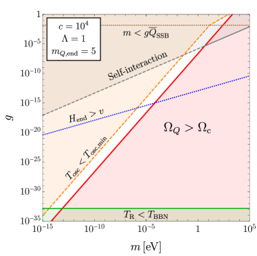
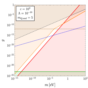
Figure 3: Abundance of vector dark matter for $c=10^{4}$ and $m_{Q,\mathrm{end}}=5$. We adopt $\Lambda=1$ and $10^{-10}$ in the left and right panels, respectively. The dark vector accounts for the observed abundance of dark matter on the red line, and the red-shaded region is excluded by over-abundance. The gray-shaded region is excluded by the constraint on self-interaction of dark matter if the dark vector accounts for all dark matter. The orange-shaded region is excluded for all dark matter because the formation of dark matter is too late. Above the red line, the gray and orange lines are shown by dashed lines because the dark vector field accounts for a part of dark matter. The green-shaded region is excluded because the reheating temperature is lower than the BBN temperature. The blue dotted line shows the typical threshold for the pre/post-inflationary scenario. Above the blue dotted line, the SU(2) symmetry is expected to be restored during inflation though the exact threshold depends on $\lambda$ and the thermal history of the dark sector. On the horizontal brown dotted line, the quadratic and quartic potential is comparable at the SSB in the post-inflationary scenario.

Self-interaction

First, we consider the self-interaction of dark matter, which is constrained by the observations of galaxy clusters through, e.g., dissociative mergers Markevitch:2003at ; Randall:2008ppe , strong lensing Meneghetti:2000gm , oscillations of the brightest cluster galaxy Kim:2016ujt ; Harvey:2018uwf , and the density profile Eckert:2022qia . The constraint is typically given by

$$\frac{\sigma}{m}\lesssim\mathcal{O}(0.1\,\text{--}\,1)\,\mathrm{cm^{2}/g}\ ,$$ (53)

where $\sigma$ is the self-scattering cross section. If the three components of the SU(2) gauge field constitute dark matter, its self-interaction is estimated as

$$\frac{\sigma}{m}\sim\frac{g^{4}}{m^{3}}$$ (54)

from the dimension analysis. Then, the conservative constraint, $\sigma/m\lesssim 1\,\mathrm{cm^{2}/g}$, is translated into a constraint on $g$ and $m$ as

$$m\gtrsim 60\,\mathrm{MeV}\times g^{4/3}\ .$$ (55)

Big-bang nucleosynthesis

The reheating temperature should be high enough for the successful big bang nucleosynthesis (BBN). Here, we require

$$T_{\mathrm{R}}>T_{\rm BBN}\simeq 10\,\mathrm{MeV}\ ,$$ (56)

which leads to

$$g >c^{3/2}\left(\frac{\pi^{2}g_{*,\mathrm{R}}}{90}\right)^{1/2}\frac{m_{Q,\mathrm{end}}^{2}}{M_{\mathrm{Pl}}^{2}}(10\,\mathrm{MeV})^{2}$$

$$\simeq 1.4\times 10^{-39}c^{3/2}\ .$$ (57)

Small-scale structures

In this scenario, the hidden gauge fields at first behave as radiation and, when the mass potential becomes important at $m\simeq g\overline{Q}$, they come to behave as non-relativistic matter. If dark matter experiences such a transition from dark radiation, it suppresses the matter perturbations on small scales. From the observations of small-scale structures, the redshift of the transition, $z_{\mathrm{T}}$, is bounded from below Sarkar:2014bca ; Corasaniti:2016epp ; Das:2020nwc . In particular, the abundance of the Milky Way satellite galaxies gives Das:2020nwc

$$z_{\mathrm{T}}>5.5\times 10^{6}\ ,$$ (58)

which corresponds to a lower bound of $T_{\mathrm{osc}}$:

$$T_{\mathrm{osc}}>T_{\mathrm{osc,min}}\simeq 1.3\times 10^{-6}\,\mathrm{GeV}\ .$$ (59)

As mentioned around Eq. (47), $\Omega_{Q,0}$ can be written as

$$\Omega_{Q,0} \simeq\Omega_{\mathrm{m},0}\frac{g_{*,\mathrm{R}}}{g_{*s,\mathrm{R}}}\frac{g_{*s,\mathrm{eq}}}{g_{*,\mathrm{eq}}}\left(\frac{g_{*s,\mathrm{osc}}}{g_{*s,\mathrm{R}}}\right)^{1/3}\frac{T_{\mathrm{osc}}}{2cT_{\mathrm{eq}}}\ .$$ (60)

By fixing the dark matter abundance as $\Omega_{Q,0}h^{2}=\Omega_{\mathrm{c},0}h^{2}=0.11933$ Planck:2018vyg , where $\Omega_{\mathrm{c},0}$ denotes the present energy fraction of cold dark matter, we obtain the lower bound on $c$ as

$$c>c_{\mathrm{min}} \equiv\frac{\Omega_{\mathrm{m},0}h^{2}}{\Omega_{\mathrm{c},0}h^{2}}\frac{g_{*,\mathrm{R}}}{g_{*s,\mathrm{R}}}\frac{g_{*s,\mathrm{eq}}}{g_{*,\mathrm{eq}}}\left(\frac{g_{*s,\mathrm{osc}}}{g_{*s,\mathrm{R}}}\right)^{1/3}\frac{T_{\mathrm{osc,min}}}{2T_{\mathrm{eq}}}$$

$$\simeq 1.1\times 10^{3}\ ,$$ (61)

in the pre-inflationary scenario or the post-inflationary scenario with $m<g\overline{Q}_{\mathrm{SSB}}$. In the post-inflationary scenario with $m>g\overline{Q}_{\mathrm{SSB}}$, the formation of dark matter is delayed until the SSB and the constraint from $z_{\mathrm{T}}$ becomes more severe.

Fate of $\Phi$

We also consider the fate of the doublet, $\Phi$. In the pre-inflationary scenario, $\Phi$ is decoupled from the visible sector, and the energy density of the dark sector apart from the homogeneous gauge field is negligible. The fate of $\Phi$ is unimportant unless it is produced thermally after inflation, which is discussed soon.

On the other hand, in the post-inflationary scenario, $\Phi$ is assumed to be thermalized with the visible sector. One possibility is through a sizable Higgs portal interaction. Assuming the $\Phi$ mass is smaller than the weak scale, which is consistent with the parameter region shown in Fig. 3, the $\Phi$ sector is thermalized until the electroweak phase transition if $\lambda_{\Phi H_{\rm SM}}^{2}T>H$ at $T\sim 100\,$GeV. This leads to $\lambda_{\Phi H_{\rm SM}}\gtrsim 10^{-8}.$ We note that the transverse modes of the gauge fields rarely thermalize because of the small gauge couplings in the parameter region of interest.

Soon after the electroweak phase transition, one finds that the $\Phi$ fields naturally decouple from the visible sector because they only interact with the standard model particles via higher dimensional terms. In this case, the four degrees of freedom of $\Phi$ decouples from the visible sector soon after the electroweak phase transition. If the quartic coupling is not very small, the entropy of the dark sector is transferred into the three degrees of freedom of the longitudinal modes of the hidden gauge fields when the temperature of the dark sector after the SSB becomes smaller than the dark Higgs mass $\sqrt{\lambda}v$. The produced hidden gauge fields behave as a relativistic component. We can estimate their contribution to dark radiation as

$$\Delta N_{\mathrm{eff}}\simeq\frac{3\times\left(\frac{10.75}{106.75}\times\frac{4}{3}\right)^{4/3}}{2\times 7/8}\simeq 0.12\ ,$$ (62)

which will be within reach of future CMB observations CMB-S4:2016ple ; CMB-HD:2022bsz . We note that the momenta of the longitudinal vector bosons contributing to $\Delta N_{\rm eff}$ are much higher than that of the coherent oscillation, and they coexist in the later Universe.

In addition, the portal coupling can be probed from the invisible decay of the standard model-like Higgs boson. In fact, when the dark Higgs boson is also light, future lepton colliders are quite powerful for probing the invisible decay of both Higgs bosons Haghighat:2022qyh .

IV Dark photon dark matter with kinetic mixing

So far, we have discussed the SU(2) vector boson as the dominant dark matter produced from the misalignment mechanisms by giving a mass from the vacuum expectation value of the SU(2) doublet. One of the vector bosons can be identified as the dark/hidden photon since the SU(2) gauge field can mix with a standard model photon through kinetic mixing by introducing a higher dimensional term:

$$\mathcal{L}\supset\frac{\kappa}{2f^{2}}\Phi^{\dagger}F^{a}_{\mu\nu}\sigma^{a}F^{\gamma}_{\mu\nu}\Phi\ ,$$ (63)

where $\kappa$ is a dimensionless coupling constant, and $F^{\gamma}$ is the field strength tensor of the standard model photon. Here, we assumed that this term is suppressed by $f$ in analogy to the $\phi F\tilde{F}$ term. When $\Phi$ acquires a nonzero expectation value, this term leads to the kinetic mixing as

$$\mathcal{L}\supset\frac{\kappa m^{2}}{g^{2}f^{2}}F^{\gamma}_{\mu\nu}F^{\mu\nu 3}\ ,$$ (64)

where we assumed $\Phi=(v,0)^{\mathrm{T}}$ without loss of generality. This term leads to the kinetic mixing between the photon and one component of the SU(2) gauge field:

$$\mathcal{L}\supset-\frac{\epsilon}{2}F_{\mu\nu}^{\gamma}F^{\mu\nu 3}\ ,\quad\epsilon\equiv-\frac{2\kappa m^{2}}{g^{2}f^{2}}\ .$$ (65)

We show the constraint from the kinetic mixing for $\kappa=1$ in Fig. 4.

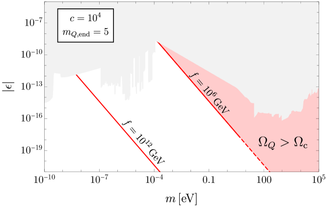
Figure 4: Kinetic mixing of the dark vector and photon. The gray-shaded region is constrained by the observations and experiments Caputo:2021eaa . Here, the constraints from the dark matter searches are shifted by $\sqrt{3}$ since only 1/3 of the dark matter mixes with the photon in this scenario. The red lines correspond to all dark matter, and the constrained region for $\Lambda=1$ is shown in the dashed lines (see Fig. 3). In the red-shaded region, the vector dark matter is overproduced.

The red lines correspond to the parameter region where the gauge field explains all dark matter, and the constrained regions are shown in the dashed lines (see Fig. 3). The kinetic mixing scales as $f^{-2}$ and can be probed by future experiments and observations depending on the value of $f$. Interestingly, the predicted kinetic mixing in the region of the post-inflationary scenario may be within reach of future experiments searching for dark photon absorption by various materials Hochberg:2016ajh ; Hochberg:2016sqx ; Bloch:2016sjj ; Hochberg:2017wce ; Knapen:2017ekk ; Chigusa:2020gfs ; Chigusa:2021mci ; Mitridate:2021ctr ; Chen:2022pyd ; Mitridate:2022tnv ; Chigusa:2023hmz . This can be also probed in LAMPOST Baryakhtar:2018doz , BREAD BREAD:2021tpx (Dish-antenna experiment Horns:2012jf ), MADMAX Gelmini:2020kcu , ALPHA Gelmini:2020kcu , and Dark E-field Godfrey:2021tvs .

We note that only 1/3 of the dark matter mixes with the photon. Since the sensitivity of the dark matter direct detection experiment is $\propto\epsilon^{2}\Omega_{\rm\gamma^{\prime}}\approx\epsilon^{2}\Omega_{\rm Q,0}/3$, we need to recast the bound/sensitivity reach of $\epsilon$ by a factor of $\sqrt{3}$. This is not the case for the astrophysics bound or tabletop experiment in which the dark photon particles are produced irrelevant to the axion-SU(2) dynamics. In other words, the difference in the sensitivity by a factor of $\sqrt{3}$ between the dark matter search, such as the haloscopes mentioned above, and tabletop experiments, such as light shining through the wall experiments Abel:2006qt ; Arias:2010bh ; Bahre:2013ywa ; Ortiz:2020tgs , can also distinguish our scenario from the other dark photon scenarios.

V Summary and discussion

We have discussed a new mechanism to generate a coherently oscillating dark vector field from the axion-SU(2) gauge field dynamics during inflation. This mechanism can evade the bounds from isocurvature perturbation, statistical anisotropy, and the ghost modes that exist in the usual misalignment production of the dark photon.

In the scenarios we have proposed, all of the SU(2) gauge fields behave as coherent oscillating dark matter while only one component, i.e., 1/3 of the total dark matter, can couple to the standard model particle via mixing. The resulting dark matter mass range can be much lighter than the eV scale and can be probed in various haloscopes as well as helioscopes and tabletop experiments. The difference by $1/\sqrt{3}$ in the mixing parameter between the searches as dark matter and other searches is a unique prediction of our scenario. In particular, the coherent oscillating vector boson that mixes with a photon has a polarization towards a fixed direction over a very large spatial scale before the structure formation. If this polarization does not change after the structure formation, the scenario predicts daily/annual modulation of the dark matter signals Caputo:2021eaa . Since the regions that can be probed from the dark photon absorption by various materials Hochberg:2016ajh ; Hochberg:2016sqx ; Bloch:2016sjj ; Hochberg:2017wce ; Knapen:2017ekk ; Chigusa:2020gfs ; Chigusa:2021mci ; Mitridate:2021ctr ; Chen:2022pyd ; Mitridate:2022tnv ; Chigusa:2023hmz and in the experiments, Super-CDMS Bloch:2016sjj , LAMPOST Baryakhtar:2018doz , BREAD BREAD:2021tpx (Dish-antenna experiment Horns:2012jf ), MADMAX Gelmini:2020kcu , ALPHA Gelmini:2020kcu , Dark E-field Godfrey:2021tvs and light shining through the wall experiments Abel:2006qt ; Arias:2010bh ; Bahre:2013ywa ; Ortiz:2020tgs is in the range of the post-inflation scenario (see Fig.3), the discovery of the hidden photon in them, together with the dark radiation of $\Delta N_{\rm eff}=\mathcal{O}(0.1)$ is another smoking-gun signal of the scenario.

In fact, the early production of the SU(2) gauge field during inflation can induce gravitational waves, and the $Q^{4}$ oscillation would have self-resonance, which also contributes to the gravitational waves. These effects, however, do not change our conclusions because the inflation scale is low.

So far, we have discussed a model for the realization of the mechanism by introducing an SU(2) doublet Higgs to break the SU(2) gauge group spontaneously. Our mechanism works in a more generic setup. For instance, we can break the SU(2) by introducing Higgs triplet(s) to give masses for the gauge boson dark matter, which leads to a more generic mass difference. In this case, we have monopoles, and the polarization of the dark photon dark matter is more non-trivial. This will be discussed elsewhere. In addition, our mechanism should even work with generic SU($N$) with $N>2$, which is also believed to have isotropic attractor solutions of homogeneous gauge field Fujita:2021eue ; Fujita:2022fff ; Murata:2022qzz . Alternatively, we can even break the SU(2) in a non-linear sigma model without introducing a Higgs field.

More generically, we can reduce the lower mass range for dark matter. This is the case if we have the gauge coupling changes effectively. The amplitude and the energy density of the vector field scales with $\overline{Q}\propto g^{-1/3}$ and $g^{2}\overline{Q}^{4}\propto g^{2/3}$ by noting the adiabatic invariant $g\overline{Q}^{3}.$ Reducing $g$ makes the comoving energy density smaller and $m$ for the transition, say $z_{\mathrm{T}}\sim 10^{7}$, smaller since the amplitude is larger. As a result, we can have the vector dark matter mass as small as the fuzzy dark matter one. The decrease of $g$ may be naturally realized from a symmetry breaking of SU(2)$\times$ SU(2)$\to$ SU(2) or from a field excursion of a moduli field relevant to the gauge coupling.

- (1) P. W. Graham, J. Mardon and S. Rajendran, Vector Dark Matter from Inflationary Fluctuations, Phys. Rev. D 93 (2016) 103520, [1504.02102].
- (2) Y. Ema, K. Nakayama and Y. Tang, Production of purely gravitational dark matter: the case of fermion and vector boson, JHEP 07 (2019) 060, [1903.10973].
- (3) A. Ahmed, B. Grzadkowski and A. Socha, Gravitational production of vector dark matter, JHEP 08 (2020) 059, [2005.01766].
- (4) E. W. Kolb and A. J. Long, Completely dark photons from gravitational particle production during the inflationary era, JHEP 03 (2021) 283, [2009.03828].
- (5) Q. Li, T. Moroi, K. Nakayama and W. Yin, Hidden dark matter from Starobinsky inflation, JHEP 09 (2021) 179, [2105.13358].
- (6) T. Sato, F. Takahashi and M. Yamada, Gravitational production of dark photon dark matter with mass generated by the Higgs mechanism, JCAP 08 (2022) 022, [2204.11896].
- (7) M. Redi and A. Tesi, Dark photon Dark Matter without Stueckelberg mass, JHEP 10 (2022) 167, [2204.14274].
- (8) Y. Tang and Y.-L. Wu, On Thermal Gravitational Contribution to Particle Production and Dark Matter, Phys. Lett. B 774 (2017) 676–681, [1708.05138].
- (9) M. Garny, A. Palessandro, M. Sandora and M. S. Sloth, Theory and Phenomenology of Planckian Interacting Massive Particles as Dark Matter, JCAP 02 (2018) 027, [1709.09688].
- (10) P. Agrawal, N. Kitajima, M. Reece, T. Sekiguchi and F. Takahashi, Relic Abundance of Dark Photon Dark Matter, Phys. Lett. B 801 (2020) 135136, [1810.07188].
- (11) R. T. Co, A. Pierce, Z. Zhang and Y. Zhao, Dark Photon Dark Matter Produced by Axion Oscillations, Phys. Rev. D 99 (2019) 075002, [1810.07196].
- (12) M. Bastero-Gil, J. Santiago, L. Ubaldi and R. Vega-Morales, Vector dark matter production at the end of inflation, JCAP 04 (2019) 015, [1810.07208].
- (13) T. Moroi and W. Yin, Light Dark Matter from Inflaton Decay, JHEP 03 (2021) 301, [2011.09475].
- (14) J. A. Dror, K. Harigaya and V. Narayan, Parametric Resonance Production of Ultralight Vector Dark Matter, Phys. Rev. D 99 (2019) 035036, [1810.07195].
- (15) K. Nakayama and W. Yin, Hidden photon and axion dark matter from symmetry breaking, JHEP 10 (2021) 026, [2105.14549].
- (16) B. Salehian, M. A. Gorji, H. Firouzjahi and S. Mukohyama, Vector dark matter production from inflation with symmetry breaking, Phys. Rev. D 103 (2021) 063526, [2010.04491].
- (17) H. Firouzjahi, M. A. Gorji, S. Mukohyama and B. Salehian, Dark photon dark matter from charged inflaton, JHEP 06 (2021) 050, [2011.06324].
- (18) Y. Nakai, R. Namba and I. Obata, Peaky production of light dark photon dark matter, JCAP 08 (2023) 032, [2212.11516].
- (19) P. Adshead, K. D. Lozanov and Z. J. Weiner, Dark photon dark matter from an oscillating dilaton, Phys. Rev. D 107 (2023) 083519, [2301.07718].
- (20) W. Yin, Thermal production of cold “hot dark matter” around eV, JHEP 05 (2023) 180, [2301.08735].
- (21) A. J. Long and L.-T. Wang, Dark Photon Dark Matter from a Network of Cosmic Strings, Phys. Rev. D 99 (2019) 063529, [1901.03312].
- (22) N. Kitajima and K. Nakayama, Dark photon dark matter from cosmic strings and gravitational wave background, JHEP 08 (2023) 068, [2212.13573].
- (23) A. E. Nelson and J. Scholtz, Dark Light, Dark Matter and the Misalignment Mechanism, Phys. Rev. D 84 (2011) 103501, [1105.2812].
- (24) P. Arias, D. Cadamuro, M. Goodsell, J. Jaeckel, J. Redondo and A. Ringwald, WISPy Cold Dark Matter, JCAP 06 (2012) 013, [1201.5902].
- (25) K. Nakayama, Vector Coherent Oscillation Dark Matter, JCAP 10 (2019) 019, [1907.06243].
- (26) N. Kitajima and K. Nakayama, Viable vector coherent oscillation dark matter, JCAP 07 (2023) 014, [2303.04287].
- (27) K. Kaneta, H.-S. Lee, J. Lee and J. Yi, Misalignment mechanism for a mass-varying vector boson, JCAP 09 (2023) 017, [2306.01291].
- (28) K. Nakayama, Constraint on Vector Coherent Oscillation Dark Matter with Kinetic Function, JCAP 08 (2020) 033, [2004.10036].
- (29) P. Adshead and M. Wyman, Chromo-Natural Inflation: Natural inflation on a steep potential with classical non-Abelian gauge fields, Phys. Rev. Lett. 108 (2012) 261302, [1202.2366].
- (30) E. Komatsu, New physics from the polarized light of the cosmic microwave background, Nature Rev. Phys. 4 (2022) 452–469, [2202.13919].
- (31) E. Dimastrogiovanni and M. Peloso, Stability analysis of chromo-natural inflation and possible evasion of Lyth’s bound, Phys. Rev. D 87 (2013) 103501, [1212.5184].
- (32) P. Adshead, E. Martinec and M. Wyman, Gauge fields and inflation: Chiral gravitational waves, fluctuations, and the Lyth bound, Phys. Rev. D 88 (2013) 021302, [1301.2598].
- (33) P. Adshead, E. Martinec and M. Wyman, Perturbations in Chromo-Natural Inflation, JHEP 09 (2013) 087, [1305.2930].
- (34) R. R. Caldwell and C. Devulder, Axion Gauge Field Inflation and Gravitational Leptogenesis: A Lower Bound on B Modes from the Matter-Antimatter Asymmetry of the Universe, Phys. Rev. D 97 (2018) 023532, [1706.03765].
- (35) I. Obata, T. Miura and J. Soda, Chromo-Natural Inflation in the Axiverse, Phys. Rev. D 92 (2015) 063516, [1412.7620].
- (36) I. Obata and J. Soda, Chiral primordial Chiral primordial gravitational waves from dilaton induced delayed chromonatural inflation, Phys. Rev. D 93 (2016) 123502, [1602.06024].
- (37) V. Domcke, B. Mares, F. Muia and M. Pieroni, Emerging chromo-natural inflation, JCAP 04 (2019) 034, [1807.03358].
- (38) T. Fujita, K. Imagawa and K. Murai, Gravitational waves detectable in laser interferometers from axion-SU(2) inflation, JCAP 07 (2022) 046, [2203.15273].
- (39) M. Czerny and F. Takahashi, Multi-Natural Inflation, Phys. Lett. B 733 (2014) 241–246, [1401.5212].
- (40) M. Czerny, T. Higaki and F. Takahashi, Multi-Natural Inflation in Supergravity, JHEP 05 (2014) 144, [1403.0410].
- (41) M. Czerny, T. Higaki and F. Takahashi, Multi-Natural Inflation in Supergravity and BICEP2, Phys. Lett. B 734 (2014) 167–172, [1403.5883].
- (42) T. Higaki, T. Kobayashi, O. Seto and Y. Yamaguchi, Axion monodromy inflation with multi-natural modulations, JCAP 10 (2014) 025, [1405.0775].
- (43) R. Daido, F. Takahashi and W. Yin, The ALP miracle: unified inflaton and dark matter, JCAP 05 (2017) 044, [1702.03284].
- (44) R. Daido, F. Takahashi and W. Yin, The ALP miracle revisited, JHEP 02 (2018) 104, [1710.11107].
- (45) F. Takahashi and W. Yin, ALP inflation and Big Bang on Earth, JHEP 07 (2019) 095, [1903.00462].
- (46) F. Takahashi and W. Yin, Challenges for heavy QCD axion inflation, JCAP 10 (2021) 057, [2105.10493].
- (47) F. Takahashi and W. Yin, Hadrophobic Axion from GUT, 2301.10757.
- (48) Y. Narita, F. Takahashi and W. Yin, QCD Axion Hybrid Inflation, 2308.12154.
- (49) K. Murai and W. Yin, A novel probe of supersymmetry in light of nanohertz gravitational waves, JHEP 10 (2023) 062, [2307.00628].
- (50) D. Croon and V. Sanz, Saving Natural Inflation, JCAP 02 (2015) 008, [1411.7809].
- (51) T. Higaki and F. Takahashi, Elliptic inflation: interpolating from natural inflation to R2-inflation, JHEP 03 (2015) 129, [1501.02354].
- (52) T. Higaki and Y. Tatsuta, Inflation from periodic extra dimensions, JCAP 07 (2017) 011, [1611.00808].
- (53) P. Adshead, E. Martinec, E. I. Sfakianakis and M. Wyman, Higgsed Chromo-Natural Inflation, JHEP 12 (2016) 137, [1609.04025].
- (54) F. Elahi and S. Khatibi, Light and feebly interacting non-Abelian vector dark matter produced through vector misalignment, Phys. Lett. B 843 (2023) 138050, [2204.04012].
- (55) E. Dimastrogiovanni, M. Fasiello and T. Fujita, Primordial Gravitational Waves from Axion-Gauge Fields Dynamics, JCAP 01 (2017) 019, [1608.04216].
- (56) A. Maleknejad and E. Erfani, Chromo-Natural Model in Anisotropic Background, JCAP 03 (2014) 016, [1311.3361].
- (57) I. Wolfson, A. Maleknejad and E. Komatsu, How attractive is the isotropic attractor solution of axion-SU(2) inflation?, JCAP 09 (2020) 047, [2003.01617].
- (58) I. Wolfson, A. Maleknejad, T. Murata, E. Komatsu and T. Kobayashi, The isotropic attractor solution of axion-SU(2) inflation: universal isotropization in Bianchi type-I geometry, JCAP 09 (2021) 031, [2105.06259].
- (59) T. Fujita, R. Namba and Y. Tada, Does the detection of primordial gravitational waves exclude low energy inflation?, Phys. Lett. B 778 (2018) 17–21, [1705.01533].
- (60) K. Ishiwata, E. Komatsu and I. Obata, Axion-gauge field dynamics with backreaction, JCAP 03 (2022) 010, [2111.14429].
- (61) Planck collaboration, N. Aghanim et al., Planck 2018 results. VI. Cosmological parameters, Astron. Astrophys. 641 (2020) A6, [1807.06209].
- (62) D. J. Fixsen, The Temperature of the Cosmic Microwave Background, Astrophys. J. 707 (2009) 916–920, [0911.1955].
- (63) N. Kitajima, S. Nakagawa and F. Takahashi, Nonthermally trapped inflation by tachyonic dark photon production, Phys. Rev. D 105 (2022) 103011, [2111.06696].
- (64) S. Nakagawa, F. Takahashi and W. Yin, Early dark energy by a dark Higgs field and axion-induced nonthermal trapping, Phys. Rev. D 107 (2023) 063016, [2209.01107].
- (65) M. Markevitch, A. H. Gonzalez, D. Clowe, A. Vikhlinin, L. David, W. Forman et al., Direct constraints on the dark matter self-interaction cross-section from the merging galaxy cluster 1E0657-56, Astrophys. J. 606 (2004) 819–824, [astro-ph/0309303].
- (66) S. W. Randall, M. Markevitch, D. Clowe, A. H. Gonzalez and M. Bradac, Constraints on the Self-Interaction Cross-Section of Dark Matter from Numerical Simulations of the Merging Galaxy Cluster 1E 0657-56, Astrophys. J. 679 (2008) 1173–1180, [0704.0261].
- (67) M. Meneghetti, N. Yoshida, M. Bartelmann, L. Moscardini, V. Springel, G. Tormen et al., Giant cluster arcs as a constraint on the scattering cross-section of dark matter, Mon. Not. Roy. Astron. Soc. 325 (2001) 435, [astro-ph/0011405].
- (68) S. Y. Kim, A. H. G. Peter and D. Wittman, In the Wake of Dark Giants: New Signatures of Dark Matter Self Interactions in Equal Mass Mergers of Galaxy Clusters, Mon. Not. Roy. Astron. Soc. 469 (2017) 1414–1444, [1608.08630].
- (69) D. Harvey, A. Robertson, R. Massey and I. G. McCarthy, Observable tests of self-interacting dark matter in galaxy clusters: BCG wobbles in a constant density core, Mon. Not. Roy. Astron. Soc. 488 (2019) 1572–1579, [1812.06981].
- (70) D. Eckert, S. Ettori, A. Robertson, R. Massey, E. Pointecouteau, D. Harvey et al., Constraints on dark matter self-interaction from the internal density profiles of X-COP galaxy clusters, Astron. Astrophys. 666 (2022) A41, [2205.01123].
- (71) A. Sarkar, S. Das and S. K. Sethi, How Late can the Dark Matter form in our universe?, JCAP 03 (2015) 004, [1410.7129].
- (72) P. S. Corasaniti, S. Agarwal, D. J. E. Marsh and S. Das, Constraints on dark matter scenarios from measurements of the galaxy luminosity function at high redshifts, Phys. Rev. D 95 (2017) 083512, [1611.05892].
- (73) S. Das and E. O. Nadler, Constraints on the epoch of dark matter formation from Milky Way satellites, Phys. Rev. D 103 (2021) 043517, [2010.01137].
- (74) CMB-S4 collaboration, K. N. Abazajian et al., CMB-S4 Science Book, First Edition, 1610.02743.
- (75) CMB-HD collaboration, S. Aiola et al., Snowmass2021 CMB-HD White Paper, 2203.05728.
- (76) G. Haghighat, M. Mohammadi Najafabadi, K. Sakurai and W. Yin, Probing a light dark sector at future lepton colliders via invisible decays of the SM-like and dark Higgs bosons, Phys. Rev. D 107 (2023) 035033, [2209.07565].
- (77) A. Caputo, A. J. Millar, C. A. J. O’Hare and E. Vitagliano, Dark photon limits: A handbook, Phys. Rev. D 104 (2021) 095029, [2105.04565].
- (78) Y. Hochberg, T. Lin and K. M. Zurek, Detecting Ultralight Bosonic Dark Matter via Absorption in Superconductors, Phys. Rev. D 94 (2016) 015019, [1604.06800].
- (79) Y. Hochberg, T. Lin and K. M. Zurek, Absorption of light dark matter in semiconductors, Phys. Rev. D 95 (2017) 023013, [1608.01994].
- (80) I. M. Bloch, R. Essig, K. Tobioka, T. Volansky and T.-T. Yu, Searching for Dark Absorption with Direct Detection Experiments, JHEP 06 (2017) 087, [1608.02123].
- (81) Y. Hochberg, Y. Kahn, M. Lisanti, K. M. Zurek, A. G. Grushin, R. Ilan et al., Detection of sub-MeV Dark Matter with Three-Dimensional Dirac Materials, Phys. Rev. D 97 (2018) 015004, [1708.08929].
- (82) S. Knapen, T. Lin, M. Pyle and K. M. Zurek, Detection of Light Dark Matter With Optical Phonons in Polar Materials, Phys. Lett. B 785 (2018) 386–390, [1712.06598].
- (83) S. Chigusa, T. Moroi and K. Nakayama, Detecting light boson dark matter through conversion into a magnon, Phys. Rev. D 101 (2020) 096013, [2001.10666].
- (84) S. Chigusa, T. Moroi and K. Nakayama, Axion/hidden-photon dark matter conversion into condensed matter axion, JHEP 08 (2021) 074, [2102.06179].
- (85) A. Mitridate, T. Trickle, Z. Zhang and K. M. Zurek, Dark matter absorption via electronic excitations, JHEP 09 (2021) 123, [2106.12586].
- (86) H.-Y. Chen, A. Mitridate, T. Trickle, Z. Zhang, M. Bernardi and K. M. Zurek, Dark matter direct detection in materials with spin-orbit coupling, Phys. Rev. D 106 (2022) 015024, [2202.11716].
- (87) A. Mitridate, T. Trickle, Z. Zhang and K. M. Zurek, Snowmass white paper: Light dark matter direct detection at the interface with condensed matter physics, Phys. Dark Univ. 40 (2023) 101221, [2203.07492].
- (88) S. Chigusa, T. Moroi, K. Nakayama and T. Sichanugrist, Dark matter detection using nuclear magnetization in magnet with hyperfine interaction, Phys. Rev. D 108 (2023) 095007, [2307.08577].
- (89) M. Baryakhtar, J. Huang and R. Lasenby, Axion and hidden photon dark matter detection with multilayer optical haloscopes, Phys. Rev. D 98 (2018) 035006, [1803.11455].
- (90) BREAD collaboration, J. Liu et al., Broadband Solenoidal Haloscope for Terahertz Axion Detection, Phys. Rev. Lett. 128 (2022) 131801, [2111.12103].
- (91) D. Horns, J. Jaeckel, A. Lindner, A. Lobanov, J. Redondo and A. Ringwald, Searching for WISPy Cold Dark Matter with a Dish Antenna, JCAP 04 (2013) 016, [1212.2970].
- (92) G. B. Gelmini, A. J. Millar, V. Takhistov and E. Vitagliano, Probing dark photons with plasma haloscopes, Phys. Rev. D 102 (2020) 043003, [2006.06836].
- (93) B. Godfrey et al., Search for dark photon dark matter: Dark E field radio pilot experiment, Phys. Rev. D 104 (2021) 012013, [2101.02805].
- (94) S. A. Abel, J. Jaeckel, V. V. Khoze and A. Ringwald, Illuminating the Hidden Sector of String Theory by Shining Light through a Magnetic Field, Phys. Lett. B 666 (2008) 66–70, [hep-ph/0608248].
- (95) P. Arias, J. Jaeckel, J. Redondo and A. Ringwald, Optimizing Light-Shining-through-a-Wall Experiments for Axion and other WISP Searches, Phys. Rev. D 82 (2010) 115018, [1009.4875].
- (96) R. Bähre et al., Any light particle search II —Technical Design Report, JINST 8 (2013) T09001, [1302.5647].
- (97) M. D. Ortiz et al., Design of the ALPS II optical system, Phys. Dark Univ. 35 (2022) 100968, [2009.14294].
- (98) T. Fujita, K. Mukaida, K. Murai and H. Nakatsuka, SU(N) natural inflation, Phys. Rev. D 105 (2022) 103519, [2110.03228].
- (99) T. Fujita, K. Murai and R. Namba, Universality of linear perturbations in SU(N) natural inflation, Phys. Rev. D 105 (2022) 103518, [2203.03977].
- (100) T. Murata, T. Fujita and T. Kobayashi, How does SU(N)-natural inflation isotropize the Universe?, Phys. Rev. D 107 (2023) 043508, [2211.09489].