An $LDL^{\mskip 1.0mu\mathrm{\scriptstyle T}}$ Trust-Region Quasi-Newton Method

Abstract

For quasi-Newton methods in unconstrained minimization, it is valuable to develop methods that are robust, i.e., methods that converge on a large number of problems. Trust-region algorithms are often regarded to be more robust than line-search methods, however, because trust-region methods are computationally more expensive, the most popular quasi-Newton implementations use line-search methods. To fill this gap, we develop a trust-region method that updates an $LDL^{\mskip 1.0mu\mathrm{\scriptstyle T}}$ factorization, scales quadratically with the size of the problem, and is competitive with a conventional line-search method.

65K10, 90C53, 65F10, 15-04

1 Introduction

Consider the unconstrained minimization problem

(1) $$\underset{x\in\mathbb{R}^{n}}{\text{ minimize}}\;\;f(x),$$

where $f:\mathbb{R}^{n}\to\mathbb{R}$ is at least twice-continuously differentiable. This problem is important for machine-learning [3], model order reduction [44], financial option pricing [1] and many related scientific and engineering problems. Second-order model-based methods for the problem generate an infinite sequence $\{x_{k}\}$ in which $x_{k+1}$ is found by minimizing a local quadratic model of $f$ based on values of the gradient $\nabla\!f(x)$ and Hessian $\nabla^{2}f(x)$ at $x_{k}$. Any method for unconstrained optimization must include a globalization strategy that forces convergence from any starting point. Broadly speaking, the two principal components of any globalization strategy are a line search and/or the solution of a trust-region subproblem. In a conventional line-search method the local quadratic model is defined in terms of the change in variables $p_{k}$. Once $p_{k}$ has been determined, a line search is used to compute a positive scalar step length $\alpha_{k}$ such that $f(x_{k}+\alpha_{k}p_{k})$ is sufficiently less than $f(x_{k})$. In this case the local quadratic model must be defined in terms of a positive-definite $\nabla^{2}f(x_{k})$ (or, a positive-definite approximation thereof) in order to ensure that the quadratic model has a bounded minimizer. By contrast, a trust-region method is designed to give a new iterate $x_{k}+s_{k}$, where $s_{k}$ is a minimizer of $\nabla\!f(x_{k})^{\mskip 1.0mu\mathrm{\scriptstyle T}}s+\tfrac{1}{2}s^{\mskip 1.0mu\mathrm{\scriptstyle T}}\nabla^{2}f(x_{k})s$ subject to the constraint $\|s\|\leq\Delta_{k}$. The value of $\Delta_{k}$ is chosen by an iterative process designed to compute a value $f(x_{k}+s_{k})$ that is sufficiently less than $f(x_{k})$. If the two-norm is used for the constraint $\|s\|\leq\Delta_{k}$ and $n$ is “small-to-medium” in size, the standard method is due to Moré & Sorensen [40]. In this method the subproblem is also solved by an iterative method, with each iteration requiring the factorization of a diagonally-shifted Hessian $\nabla^{2}f(x_{k})+\sigma_{j}I$ for $\sigma_{j}$ a nonnegative scalar. In general, the Moré-Sorensen method requires several factorizations to find $s_{k}$. However, this cost is mitigated by the fact that compared to line-search methods, trust-region methods have a stronger convergence theory and are generally more robust, i.e., they are able to solve more problems (see e.g., Dai [16], Gay [24], Sorensen [46], Hebden [35], and Conn, Gould & Toint [15]).

If first derivatives, but not second derivatives are available, then quasi-Newton methods can be very effective (see, e.g., Dennis & Moré [17], Gill & Murray [27], Byrd, Dong & Nocedal [13]). Quasi-Newton methods maintain an approximate Hessian $B_{k}$ (or approximate inverse Hessian $H_{k}$) that is modified by a low-rank update that installs the curvature information accumulated in the step from $x_{k}$ to $x_{k+1}$. By updating $H_{k}$ or a factorization of $B_{k}$, a quasi-Newton method can be implemented in $O(n^{2})$ floating-point operations (flops) per iteration. There are infinitely many possible modifications, but it can be argued that the most widely used quasi-Newton method is the Broyden-Fletcher-Goldfarb-Shanno (BFGS) method (see Broyden [4], Fletcher [21], Goldfarb [30] and Shanno [45]), which uses a rank-two update. This method has exhibited superior performance in a large number of comparisons (see, Gill & Runnoe [29] for a recent survey). In particular, many state-of-the-art software implementations include an option to use a quasi-Newton method, see, e.g., SNOPT [28], IPOPT [49], Knitro [14] and the Matlab Optimization ToolBox [39]. All these implementations use the BFGS method in conjunction with a Wolfe line-search (see, e.g., Moré & Thuente [41]). In particular, if $B_{k}$ is positive definite and the Wolfe line-search conditions hold, then the update gives a positive-definite matrix and the method typically exhibits a fast superlinear convergence rate. A method based on the BFGS update is the focus of Section 3. However, we start by making no assumptions about the method used to compute $B_{k}$.

Although trust-region globalization methods tend to provide a more reliable algorithm overall, the additional factorizations required at each iteration have limited their application to quasi-Newton methods. The trust-region subproblem for the quasi-Newton case is given by

(2) $$\underset{\|s\|\leq\Delta_{k}}{\mathrm{minimize}}\;\;g_{k}^{\mskip 1.0mu\mathrm{\scriptstyle T}}s+\tfrac{1}{2}s^{\mskip 1.0mu\mathrm{\scriptstyle T}}B_{k}s,$$

where $\Delta_{k}$ is the positive trust-region radius, $g_{k}$ is the gradient $\nabla\!f(x_{k})$, and $B_{k}$ is an $n\times n$ symmetric quasi-Newton approximation to the Hessian matrix $\nabla^{2}f(x_{k})$. The trust-region subproblem (2) can be solved using the Moré-Sorensen method, but the substantial cost of repeatedly factoring a shifted approximate Hessian has motivated the formulation of less expensive methods for computing $s_{k}$. The most successful of these methods are based on a combination of three basic strategies.

The first strategy is to choose the norm of $s$ so that the subproblem (2) is easier to solve. In Gertz [25] the trust-region constraint is defined in terms of the infinity-norm and the associated trust-region subproblem is solved using a quadratic programming algorithm. An infinity-norm trust-region is also the basis of Fletcher’s S$l_{1}$QP method for constrained optimization (see Fletcher [22]).

The second strategy is to use an iterative method to solve the linear equations associated with the optimality conditions for problem (2). Iterative methods have the benefit of being able to compute approximate solutions of (2). Steihaug [47] and Toint [48] apply the conjugate-gradient method to the equations $B_{k}s=-g_{k}$ but terminate the iterations if a direction of negative curvature is detected or the trust-region constraint becomes active.

The third strategy is to seek an approximate solution of (2) that lies in a low-dimensional subspace (of dimension less than 10, say). The dogleg method of Powell [42] uses the subspace spanned by the vectors $\{g_{k},B_{k}^{-1}g_{k}\}$. Byrd, Schnabel and Schultz [12] propose using the subspace based on $\{g_{k},(B_{k}+\sigma I)^{-1}g_{k}\}$ for some nonnegative $\sigma$. This extends the dogleg method to the case where $B_{k}$ is not positive definite.

Other well-known iterative trust-region methods have been proposed that do not use a quasi-Newton approximate Hessian. These include the SSM (Hager [34]), GLTR (Gould, Lucidi, Roma & Toint [32]) and Algorithm 4 of Erway, Gill & Griffin [20].

A number of methods combine the three strategies described above. These include the methods of Brust, Marcia, Petra & Saunders [9] and Brust, Marcia & Petra [8]. The use of a trust-region approach in conjunction with a limited-memory approximate Hessian has been developed in Brust, Burdakov, Erway & Marcia [7].

The proposed method is based on exploiting the properties of the factorization

(3) $$B_{k}=L_{k}D_{k}L_{k}^{\mskip 1.0mu\mathrm{\scriptstyle T}},$$

where $L_{k}\in\mathbb{R}^{n\times n}$ is lower triangular and $D_{k}\in\mathbb{R}^{n\times n}$ is diagonal. This factorization and the associated Cholesky factorization have been used extensively in the implementation of line-search quasi-Newton methods (see, e.g., Gill & Murray [27], Fletcher & Powell [23], Dennis & Schnabel [18]) but they are seldom used in trust-region quasi-Newton methods. In Luksan [37] a factorization similar to (3) is used for nonlinear least-squares, by introducing transformed trust-region constraints $\|L_{k}^{\mskip 1.0mu\mathrm{\scriptstyle T}}s\|\leq\Delta_{k}$ in the subproblem. However, it is not applied to general minimization problems.

1.1 Contributions

We formulate and analyze a quasi-Newton trust-region method based on exploiting the properties of the $LDL^{\mskip 1.0mu\mathrm{\scriptstyle T}}$ factorization. Each iteration involves two phases. In the first phase we use a strategy similar to that proposed by Luksan [37] that computes an inexpensive scalar diagonal shift for $B_{k}$ based on solving a trust-region subproblem with a diagonal matrix $D_{k}$. In the second phase the computed shift and the factorization in (3) are used to define an effective conjugate-gradient iteration. These steps give a quasi-Newton trust-region algorithm that is competitive with state-of-the-art line-search implementations. We note that Gould, Lucidi, Roma & Toint [32] have anticipated the potential of a two-phased approached, however, to the best of our knowledge, the proposed method is new.

1.2 Notation

We use Householder notation, which uses upper- and lower-case Roman letters to represent matrices and vectors, and lower-case Greek symbols to represent scalars. The one exception to this rule is $\Delta_{k}>0$, which denotes a scalar. The identity matrix is $I$ with dimension depending on the context. The subscript $k$ ($k\geq 0$) represents the main iteration index. At times, an inner-iteration will be used, which is denoted by a superscript. For example, a matrix used in inner iteration $j$ of outer iteration $k$ is denoted by $Q^{(j)}_{k}$. The letters $D_{k}$ and $E_{k}$ are reserved for diagonal matrices and $R_{k}$, $L_{k}$ and $T_{k}$ denote triangular matrices.

2 The Method

The proposed method is based on exploiting the properties of the factorization (3). First, we show how a low-rank modification of the factors can be updated in $O(n^{2})$ operations.

2.1 Updates to the factors

Suppose that the factorization $B_{k}=L_{k}D_{k}L_{k}^{\mskip 1.0mu\mathrm{\scriptstyle T}}$ is available at the start of the $k$th iteration. We make no assumptions concerning whether or not $B_{k}$ is positive definite but $L_{k}$ is assumed to be nonsingular. We wish to compute $L_{k+1}$ and $D_{k+1}$ following a rank-one update to $B_{k}$. In particular, consider

(4) $$L_{k}D_{k}L^{\mskip 1.0mu\mathrm{\scriptstyle T}}_{k}+\alpha_{k}a_{k}a^{\mskip 1.0mu\mathrm{\scriptstyle T}}_{k}=L_{k+1}D_{k+1}L_{k+1}^{\mskip 1.0mu\mathrm{\scriptstyle T}},$$

where $a_{k}\in\mathbb{R}^{n}$ and $\alpha_{k}\in\mathbb{R}$. Let ${\bar{L\mkern 4.3mu}\mkern-4.3mu}{}^{(1)}_{k}$ denote the $n\times(n+1)$ matrix $\begin{bmatrix}L_{k}&a_{k}\end{bmatrix}$, which is lower triangular except for its last column. Similarly, let $\bar{D}^{(1)}_{k}$ denote the $(n+1)\times(n+1)$ diagonal matrix $\operatorname{diag}(D_{k},\alpha_{k})$. Then

$$L_{k}D_{k}L^{\mskip 1.0mu\mathrm{\scriptstyle T}}_{k}+\alpha_{k}a_{k}a^{\mskip 1.0mu\mathrm{\scriptstyle T}}_{k}=\begin{bmatrix}L_{k}&a_{k}\end{bmatrix}\begin{bmatrix}D_{k}&\\ &\alpha_{k}\end{bmatrix}{\begin{bmatrix}L_{k}&a_{k}\end{bmatrix}}^{\mskip 1.0mu\mathrm{\scriptstyle T}}={\bar{L\mkern 4.3mu}\mkern-4.3mu}{}^{(1)}_{k}\bar{D}^{(1)}_{k}{{\bar{L\mkern 4.3mu}\mkern-4.3mu}{}^{(1)}_{k}}{}^{\mskip 1.0mu\mathrm{\scriptstyle T}}.$$

A sequence of orthogonal Given’s rotations $Q^{(1)}_{k}\cdots Q^{(n)}_{k}$ may be used to zero out the elements of the last column in ${\bar{L\mkern 4.3mu}\mkern-4.3mu}{}^{(1)}_{k}$ (cf. Golub & Van Loan [31]). For $j=1$, $2$, …, $n$ we define

(5) $${\bar{L\mkern 4.3mu}\mkern-4.3mu}{}^{(j+1)}_{k}={\bar{L\mkern 4.3mu}\mkern-4.3mu}{}^{(j)}_{k}Q^{(j)}_{k},$$

where each $Q^{(j)}_{k}$ is an $(n+1)\times(n+1)$ identity matrix except for four entries:

$$Q^{(j)}_{k}(j,j)=Q^{(j)}_{k}(n+1,n+1)=\frac{{\bar{L\mkern 4.3mu}\mkern-4.3mu}{}^{(j)}_{k}(j,j)}{\sqrt{({\bar{L\mkern 4.3mu}\mkern-4.3mu}{}^{(j)}_{k}(j,j))^{2}+({\bar{L\mkern 4.3mu}\mkern-4.3mu}{}^{(j)}_{k}(j,n+1))^{2}}}$$

and

$$Q^{(j)}_{k}(j,n+1)=-Q^{(j)}_{k}(n+1,j)=\frac{-{\bar{L\mkern 4.3mu}\mkern-4.3mu}{}^{(j)}_{k}(n,n+1)}{\sqrt{({\bar{L\mkern 4.3mu}\mkern-4.3mu}{}^{(j)}_{k}(j,j))^{2}+({\bar{L\mkern 4.3mu}\mkern-4.3mu}{}^{(j)}_{k}(n,n+1))^{2}}}.$$

The following example illustrates how ${\bar{L\mkern 4.3mu}\mkern-4.3mu}{}^{(1)}_{k}$ is restored to triangular form:

$$\begin{bmatrix}\times&&&&&\times\\ \times&\times&&&&\times\\ \times&\times&\times&&&\times\\ \times&\times&\times&\times&&\times\\ \times&\times&\times&\times&\times&\times\\ \end{bmatrix}Q^{(1)}_{k} =\begin{bmatrix}\times&&&&&0\\ \times&\times&&&&\times\\ \times&\times&\times&&&\times\\ \times&\times&\times&\times&&\times\\ \times&\times&\times&\times&\times&\times\\ \end{bmatrix}$$

$$\begin{bmatrix}\times&&&&&\times\\ \times&\times&&&&\times\\ \times&\times&\times&&&\times\\ \times&\times&\times&\times&&\times\\ \times&\times&\times&\times&\times&\times\\ \end{bmatrix}Q^{(1)}_{k}Q^{(2)}_{k} =\begin{bmatrix}\times&&&&&0\\ \times&\times&&&&0\\ \times&\times&\times&&&\times\\ \times&\times&\times&\times&&\times\\ \times&\times&\times&\times&\times&\times\\ \end{bmatrix}$$

$$\hskip 56.9055pt\vdots \hskip 56.9055pt\vdots$$

$$\begin{bmatrix}\times&&&&&\times\\ \times&\times&&&&\times\\ \times&\times&\times&&&\times\\ \times&\times&\times&\times&&\times\\ \times&\times&\times&\times&\times&\times\\ \end{bmatrix}Q^{(1)}_{k}Q^{(2)}_{k}\cdots Q^{(n)}_{k} =\begin{bmatrix}\times&&&&&0\\ \times&\times&&&&0\\ \times&\times&\times&&&0\\ \times&\times&\times&\times&&0\\ \times&\times&\times&\times&\times&0\\ \end{bmatrix}.$$

In general, ${\bar{L\mkern 4.3mu}\mkern-4.3mu}{}^{(n+1)}_{k}={\bar{L\mkern 4.3mu}\mkern-4.3mu}{}^{(1)}_{k}Q^{(1)}_{k}\cdots Q^{(n)}_{k}\equiv\begin{bmatrix}L_{k+1}&0\end{bmatrix}$, and $L_{k+1}$ is the first $n$ rows and columns of ${\bar{L\mkern 4.3mu}\mkern-4.3mu}{}^{(n+1)}_{k}$. A similar recursion can be applied symmetrically to $\bar{D}^{(1)}_{k}$ to give

$$\bar{D}^{(n+1)}_{k}=(Q^{(1)}_{k}Q^{(2)}_{k}\cdots Q^{(n)}_{k})^{\mskip 1.0mu\mathrm{\scriptstyle T}}\bar{D}^{(1)}_{k}Q^{(1)}_{k}Q^{(2)}_{k}\cdots Q^{(n)}_{k}\equiv\begin{bmatrix}D_{k+1}&\times\\ \times&\times\end{bmatrix}.$$

If the product $Q^{(1)}_{k}Q^{(2)}_{k}\cdots Q^{(n)}_{k}$ is denoted by $Q_{k}$ then the factorization can be written as

(6) $$\left\{\begin{aligned} \;\;L_{k}D_{k}L^{\mskip 1.0mu\mathrm{\scriptstyle T}}_{k}+\alpha_{k}a_{k}a^{\mskip 1.0mu\mathrm{\scriptstyle T}}_{k}&={\bar{L\mkern 4.3mu}\mkern-4.3mu}{}^{(1)}_{k}\bar{D}^{(1)}_{k}{{\bar{L\mkern 4.3mu}\mkern-4.3mu}{}^{(1)}_{k}}{}^{\mskip 1.0mu\mathrm{\scriptstyle T}}={\bar{L\mkern 4.3mu}\mkern-4.3mu}{}^{(1)}_{k}Q_{k}Q^{\mskip 1.0mu\mathrm{\scriptstyle T}}_{k}\bar{D}^{(1)}_{k}Q_{k}Q^{\mskip 1.0mu\mathrm{\scriptstyle T}}_{k}{{\bar{L\mkern 4.3mu}\mkern-4.3mu}{}^{(1)}_{k}}{}^{\mskip 1.0mu\mathrm{\scriptstyle T}}\\ &=L_{k+1}D_{k+1}L_{k+1}^{\mskip 1.0mu\mathrm{\scriptstyle T}}.\end{aligned}\right.$$

If $B_{k}$ is not positive definite, then some of the elements of $D_{k+1}$ may be negative or zero and some diagonal elements of $L_{k+1}$ may be zero. In the latter case any offending diagonals of $L_{k+1}$ must be modified to give a nonsingular factor for the next iteration.

Because of the special form of each Given’s rotation $Q^{(j)}_{k}$, each product in (5) can be computed with $O(n)$ flops. As there are $n$ total products, updating the indefinite factorization with a rank-one term requires $O(n^{2})$ flops. If more than one rank-one update is required, the method can be applied as many times as needed. A related algorithm for updating the Cholesky factorization is given in Algorithm C1 of Gill, Golub, Murray & Saunders [26].

2.2 Computing the optimal shift

Trust-region methods generate a sequence of solution estimates $\{x_{k}\}$ such that $x_{k+1}=x_{k}+s_{k}$, where $s_{k}\in\mathbb{R}^{n}$ is a solution of the trust-region subproblem (2). If the two-norm is used to define the trust region then $s^{\ast}$ is a global minimizer of the trust-region subproblem if and only if $\|s^{\ast}\|_{2}\leq\Delta_{k}$ and there is a scalar “shift” $\sigma^{\ast}\geq 0$ such that

(7) $$(B_{k}+\sigma^{\ast}I)s^{\ast}=-g_{k}\;\;\text{and}\;\;\sigma^{\ast}(\Delta_{k}-\|s^{\ast}\|_{2})=0,$$

with $B_{k}+\sigma^{\ast}I$ positive semidefinite. Moreover, if $B_{k}+\sigma^{\ast}I$ is positive definite, then the global minimizer is unique. Once the optimal “shift” $\sigma^{\ast}\geq 0$ is known, determining $s^{\ast}$ reduces to solving the shifted linear system $(B_{k}+\sigma^{\ast}I)s^{\ast}=-g_{k}$. An effective algorithm due to Moré and Sorensen [40] is based on using Newton’s method to find a zero of the scalar-valued function $\varphi(\sigma)$ such that

(8) $$\varphi(\sigma)\equiv\frac{1}{\Delta_{k}}-\frac{1}{\|s\|_{2}},\quad\text{where}\quad(B_{k}+\sigma I)s=-g_{k}.$$

Starting with a nonnegative scalar $\sigma_{0}$ such that $B_{k}+\sigma_{0}I$ is positive semidefinite, each iteration of Newton’s method requires the computation of the Cholesky factorization $R^{\mskip 1.0mu\mathrm{\scriptstyle T}}_{i}R_{i}=B_{k}+\sigma_{i}I$. The main computational steps of the Moré-Sorensen method are summarized in Algorithm 1.

Algorithm $\mskip-3.5mu\bf{1}$

$\sigma_{0}\geq 0$;   $R_{0}$ such that $R_{0}^{\mskip 1.0mu\mathrm{\scriptstyle T}}R_{0}=B_{k}+\sigma_{0}I$;

for $i=0\,{:}\,i_{\mathrm{max}}$ do

     Solve $R_{i}^{\mskip 1.0mu\mathrm{\scriptstyle T}}R_{i}s_{i}=-g_{k}$;

     Solve $R_{i}^{\mskip 1.0mu\mathrm{\scriptstyle T}}q_{i}=s_{i}$;

     Update $\sigma_{i+1}=\sigma_{i}+\dfrac{\|s_{i}\|_{2}^{2}}{\|q_{i}\|_{2}^{2}}\Big{(}\dfrac{\|s_{i}\|_{2}-\Delta_{k}}{\Delta_{k}}\Big{)}$;

     Factor $R_{i+1}^{\mskip 1.0mu\mathrm{\scriptstyle T}}R_{i+1}=B_{k}+\sigma_{i+1}I$;

end for;

This iteration typically continues until $\|s_{i}\|_{2}\approx\Delta_{k}$. Recomputing the factorization $R_{i+1}^{\mskip 1.0mu\mathrm{\scriptstyle T}}R_{i+1}$ is by far the most expensive part of the algorithm. Therefore, practical implementations typically first check whether the solution to $B_{k}s_{0}=-g_{k}$ satisfies $\|s_{0}\|_{2}\leq\Delta_{k}$ whenever it is known that $B_{k}$ is positive definite to avoid this loop.

2.3 Computing the modified shift (phase 1)

Since computing the optimal shift and step using Algorithm 1 is expensive, the factorization $B_{k}=L_{k}D_{k}L_{k}^{\mskip 1.0mu\mathrm{\scriptstyle T}}$ is used to compute a modified shift at a significantly reduced cost. This computation constitutes phase 1 of the proposed method. Let $T_{k}$ denote the inverse of $L_{k}^{\mskip 1.0mu\mathrm{\scriptstyle T}}$, i.e.,

$$L_{k}^{\mskip 1.0mu\mathrm{\scriptstyle T}}T_{k}=T_{k}L_{k}^{\mskip 1.0mu\mathrm{\scriptstyle T}}=I.$$

For any scalar $\sigma$ it holds that

(9) $$B_{k}+\sigma I=L_{k}D_{k}L_{k}^{\mskip 1.0mu\mathrm{\scriptstyle T}}+\sigma I=L_{k}(D_{k}+\sigma T_{k}^{\mskip 1.0mu\mathrm{\scriptstyle T}}T_{k})L_{k}^{\mskip 1.0mu\mathrm{\scriptstyle T}}.$$

This identity can be used to modify the iteration (8) so that expensive refactorizations are not needed. If $E_{k}$ is the diagonal matrix

(10) $$E_{k}=\operatorname{diag}(T_{k}^{\mskip 1.0mu\mathrm{\scriptstyle T}}T_{k}),$$

then $E_{k}$ can be used to approximate $T_{k}^{\mskip 1.0mu\mathrm{\scriptstyle T}}T_{k}$ in the conditions (7). This gives a modified shift $\sigma^{+}$ such that

(11) $$\|s^{+}\|_{2}\leq\Delta_{k},\quad L_{k}(D_{k}+\sigma^{+}E_{k})L_{k}^{\mskip 1.0mu\mathrm{\scriptstyle T}}s^{+}=-g_{k}\quad\text{and}\quad\sigma^{+}(\|s^{+}\|_{2}-\Delta_{k})=0,$$

with $D_{k}+\sigma^{+}E_{k}$ positive semidefinite. It is important to note that $D_{k}+\sigma^{+}E_{k}$ is diagonal, which allows the conditions (11) to be satisfied without the need for additional factorizations. The corresponding algorithm, with the initial scalar $\sigma^{+}_{0}\geq 0$ is given in Algorithm 2 (details of the derivation of Algorithm 2 are given in Appendix A).

Algorithm $\mskip-3.5mu\bf 2$

$\sigma^{+}_{0}\geq 0$;

for $i=0\,{:}\,i_{\mathrm{max}}$ do

     Solve $L_{k}(D_{k}+\sigma^{+}_{i}E_{k})L_{k}^{\mskip 1.0mu\mathrm{\scriptstyle T}}s^{+}_{i}=-g_{k}$;

     Solve $(D_{k}+\sigma^{+}_{i}E_{k})L_{k}^{\mskip 1.0mu\mathrm{\scriptstyle T}}q^{\scriptscriptstyle+}_{i}=-E_{k}L_{k}^{\mskip 1.0mu\mathrm{\scriptstyle T}}s^{+}_{i}$;

     Update $\sigma^{+}_{i+1}=\sigma^{+}_{i}-\dfrac{\|s^{+}_{i}\|_{2}^{2}}{s^{+}_{i}{}^{\mskip 1.0mu\mathrm{\scriptstyle T}}q^{\scriptscriptstyle+}_{i}}\Big{(}\dfrac{\|s^{+}_{i}\|_{2}-\Delta_{k}}{\Delta_{k}}\Big{)}$;

end for;

Observe that Algorithm 2 requires no direct factorizations. Moreover, the solves are inexpensive because they involve only triangular or diagonal matrices. Even though the main focus of Algorithm 2 is to compute a appropriate shift $\sigma^{+}_{i}\geq 0$, the vector $s^{+}_{i}$ is available as a by-product of the computation of $\sigma^{+}$. The vector $s^{+}_{i}$ satisfies $\|s^{+}_{i}\|_{2}=\|s^{\ast}\|_{2}=\Delta_{k}$ and is used to approximate $s^{\ast}$.

2.4 Solving the shifted system (phase 2)

The estimate $\sigma^{+}_{i}$ is expected to be an overestimate to $\sigma^{\ast}$ because $\|E_{k}\|_{2}\leq\|T_{k}^{\mskip 1.0mu\mathrm{\scriptstyle T}}T_{k}\|_{2}$. Nevertheless, it contains the exact diagonal for the optimal system by (10) and typically captures at least the right order of magnitude. For comparison, $s^{\ast}$ is the solution to the shifted system $(L_{k}D_{k}L_{k}^{\mskip 1.0mu\mathrm{\scriptstyle T}}+\sigma^{\ast}I)s^{\ast}=-g_{k}$. We use the inexpensive estimate $\sigma^{+}_{i}$ to solve the related shifted system in a second phase

(12) $$(L_{k}D_{k}L_{k}^{\mskip 1.0mu\mathrm{\scriptstyle T}}+\sigma^{+}_{i}I)s_{k}=-g_{k}.$$

The computation of an exact solution of (12) requires a factorization of $L_{k}D_{k}L_{k}^{\mskip 1.0mu\mathrm{\scriptstyle T}}+\sigma^{+}_{i}I$ and would be too expensive. Instead we propose the use of an iterative solver in combination with the $LDL^{\mskip 1.0mu\mathrm{\scriptstyle T}}$ factors. From (9) it holds that $L_{k}D_{k}L_{k}^{\mskip 1.0mu\mathrm{\scriptstyle T}}+\sigma^{+}_{i}I=L_{k}(D_{k}+\sigma^{+}_{i}T_{k}^{\mskip 1.0mu\mathrm{\scriptstyle T}}T_{k})L_{k}^{\mskip 1.0mu\mathrm{\scriptstyle T}}$. The conjugate-gradient (CG) method of Hestenes [36] can be applied to exploit the availability of the factors:

(13) $$L_{k}h_{k} =-g_{k}, (\text{triangular solve})$$

(14) $$(D_{k}+\sigma^{+}_{i}T_{k}^{\mskip 1.0mu\mathrm{\scriptstyle T}}T_{k})v_{k} =h_{k}, (\text{conjugate-gradient solve})$$

(15) $$L_{k}^{\mskip 1.0mu\mathrm{\scriptstyle T}}s_{k} =v_{k}. (\text{triangular solve})$$

This vector is often close to $s^{\ast}$ and constitutes a useful search direction.

2.5 Backtracking the shift

As $E_{k}$ is just an estimate of $T_{k}^{\mskip 1.0mu\mathrm{\scriptstyle T}}T_{k}$ the computed shift $\sigma^{+}$ is usually different from $\sigma^{\ast}$. In particular, the computed $\sigma^{+}$ is often larger than $\sigma^{\ast}$ because $\|E_{k}\|_{2}\leq\|T_{k}^{\mskip 1.0mu\mathrm{\scriptstyle T}}T_{k}\|_{2}$. In order to improve the accuracy of $\sigma^{+}$, a backtracking mechanism is included to allow additional trial values for $\sigma^{+}$. Specifically, the value of $\sigma^{+}$ is reduced as long as the function value decreases. This approach is summarized in Algorithm 3.

Algorithm $\mskip-3.5mu\bf 3$

$\sigma^{+}_{0}\geq 0$, $\gamma_{k}<1$;

Set $i=0$;

repeat

     Solve $(L_{k}D_{k}L_{k}^{\mskip 1.0mu\mathrm{\scriptstyle T}}+\sigma^{+}_{i}I)s_{k}=-g_{k}$; [Use eqs. (13)—(15)]

     $\sigma^{+}_{i+1}=\gamma_{k}\sigma^{+}_{i}$;   $i=i+1$;

until $f(x_{k})\leq f(x_{k}+s_{k})$;

The search on the shift parameter is the same for both an estimated and optimal shift, i.e., the backtracking scheme could be applied if Algorithm 1 is used to solve the subproblem. As in a backtracking line search, this strategy requires additional function evaluations. However the quality of the computed search direction is improved. For additional efficiency, the value of $\sigma^{+}_{0}$ in Algorithm 3 is set to the final estimate of $\sigma^{\ast}$ computed by Algorithm 2. Thus on initialization, $\sigma^{+}_{0}\approx\sigma^{\ast}$, but as long as $f$ decreases $\sigma^{+}_{i+1}\to 0$, and the computed steps $s_{k}$ become closer to the full quasi-Newton step $B_{k}s_{k}=-g_{k}$. Algorithm 3 is illustrated on two problems in Fig. 1, and shows that the computed $\sigma^{+}$ can often be effective even when compared to the optimal shift.

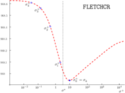
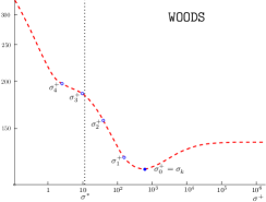
Figure 1: Illustration of Alg. 3 on the two CUTEst problems FLETCHCR and WOODS. The dashed red curve represents the objective value as a function of $\sigma^{+}$. The dotted vertical line represents the optimal shift $\sigma^{*}$. The blue point is the selected shift.

2.6 The quasi-Newton matrix

The method can be implemented by either updating the factorization $B_{k}=L_{k}D_{k}L_{k}^{\mskip 1.0mu\mathrm{\scriptstyle T}}$ directly, or by updating its inverse. For the latter approach, recall that $T_{k}$ represents the inverse of $L_{k}^{\mskip 1.0mu\mathrm{\scriptstyle T}}$, and suppose that $D_{k}$ is an invertible diagonal with inverse $G_{k}$. Then

$$D_{k}G_{k}=G_{k}D_{k}=I.$$

and

$$\big{(}L_{k}D_{k}L_{k}^{\mskip 1.0mu\mathrm{\scriptstyle T}}\big{)}{}^{-1}=L_{k}^{-\mathrm{\scriptstyle T}}D_{k}^{-1}L_{k}^{-1}=T_{k}G_{k}T_{k}^{\mskip 1.0mu\mathrm{\scriptstyle T}}.$$

It will become evident that only $T_{k}$ and $D_{k}$ need be stored when the inverse factorization is updated. Specifically, the proposed method generates two types of equation, with each equation associated with a particular phase. In phase 1, we solve a sequence of linear equations of the form

(16) $$L_{k}\big{(}D_{k}+\sigma^{+}_{i}E_{k}\big{)}L_{k}^{\mskip 1.0mu\mathrm{\scriptstyle T}}s^{+}=-g_{k}.$$

This solution can be expressed directly using only $T_{k}$, $D_{k}$ and $E_{k}$; namely, from

$$h_{k}=-T_{k}^{\mskip 1.0mu\mathrm{\scriptstyle T}}g_{k},\quad w_{k}=(D_{k}+\sigma^{+}_{i}E_{k})^{-1}h_{k},\quad s^{+}=T_{k}w_{k}.$$

Similarly, in the second phase of the method we solve systems of the form

$$L_{k}(D_{k}+\sigma^{+}T_{k}^{\mskip 1.0mu\mathrm{\scriptstyle T}}T_{k})L_{k}^{\mskip 1.0mu\mathrm{\scriptstyle T}}s_{k}=-g_{k}.$$

The solution of this system may also be computed using only $T_{k}$ and $D_{k}$. In particular,

(17) $$h_{k} =-T_{k}^{\mskip 1.0mu\mathrm{\scriptstyle T}}g_{k}, (\text{matrix-vector multiply})$$

(18) $$(D_{k}+\sigma^{+}_{i}T_{k}^{\mskip 1.0mu\mathrm{\scriptstyle T}}T_{k})v_{k} =h_{k}, (\text{conjugate-gradient solve})$$

(19) $$s_{k} =T_{k}v_{k}. (\text{matrix-vector multiply})$$

To highlight a significant difference between updating the direct factorization $L_{k}D_{k}L_{k}^{\mskip 1.0mu\mathrm{\scriptstyle T}}$ and updating the inverse factorization $T_{k}^{\mskip 1.0mu\mathrm{\scriptstyle T}}G_{k}T_{k}$ observe that the direct method computes the step in phase 2 using the equations (13)–(15).These relations depend not only on $L_{k}$ and $D_{k}$ but also $T_{k}$. Therefore, in order to implement the direct factorization it is necessary to update $L_{k}$, $D_{k}$ and $T_{k}$. In contrast, if the inverse factorization is used, the step in phase 2 is determined by (17)–(19), which depend only on $T_{k}$ and $D_{k}$. Therefore, updating the inverse factorization is advantageous from an implementation viewpoint because it depends only on $T_{k}$ and $D_{k}$. Moreover, as $D_{k}$ is diagonal it is straightforward to update $T_{k}$ and $G_{k}$, where $G_{k}$ is the inverse of $D_{k}$. The inverse quasi-Newton matrix is denoted by $H_{k}$, i.e.,

$$B_{k}^{-1}=(L_{k}D_{k}L_{k}^{\mskip 1.0mu\mathrm{\scriptstyle T}})^{-1}=T_{k}G_{k}T_{k}^{\mskip 1.0mu\mathrm{\scriptstyle T}}\equiv H_{k}.$$

The approximate Hessian and its inverse can be positive definite or indefinite depending on the choice of updating formula. The most popular updates are defined in terms of the vectors $s_{k}=x_{k+1}-x_{k}$ and $y_{k}=g_{k+1}-g_{k}$. In particular the BFGS modified inverse Hessian is given by the rank-two formula

(20) $$H_{k+1}=H_{k}+\frac{y_{k}^{\mskip 1.0mu\mathrm{\scriptstyle T}}s_{k}+y_{k}^{\mskip 1.0mu\mathrm{\scriptstyle T}}H_{k}y_{k}}{(y_{k}^{\mskip 1.0mu\mathrm{\scriptstyle T}}s_{k})^{2}}s_{k}s_{k}^{\mskip 1.0mu\mathrm{\scriptstyle T}}-\frac{1}{y_{k}^{\mskip 1.0mu\mathrm{\scriptstyle T}}s_{k}}(H_{k}y_{k}s_{k}^{\mskip 1.0mu\mathrm{\scriptstyle T}}+s_{k}y_{k}^{\mskip 1.0mu\mathrm{\scriptstyle T}}H_{k}),$$

and the SR1 inverse is

(21) $$H_{k+1}=H_{k}+\frac{1}{(y_{k}-H_{k}s_{k})^{\mskip 1.0mu\mathrm{\scriptstyle T}}s_{k}}(y_{k}-H_{k}s_{k})(y_{k}-H_{k}s_{k})^{\mskip 1.0mu\mathrm{\scriptstyle T}}.$$

Other options are the Multipoint Symmetric Secant Matrix (MSS) update of Brust [6] and Burdakov, Martínez & Pilotta [11], or the Powell-Symmetric-Broyden (PSB) update Powell [43] and Broyden, Dennis & Moré [5]. After extensive experimentation, it was found that a quasi-Newton method based on the BFGS update (20) required the fewest function evaluations (see also Gill and Runnoe [29]). For this reason, the following discussion will focus on the properties of a BFGS trust-region method.

Given the factorization $T_{k}G_{k}T_{k}^{\mskip 1.0mu\mathrm{\scriptstyle T}}$, the product $T_{k+1}G_{k+1}T_{k+1}^{\mskip 1.0mu\mathrm{\scriptstyle T}}$ is computed using a similar approach to that used in Section 2.1. In particular, for the BFGS update (20) we have

$$\alpha_{k}^{(1)} =\frac{y_{k}^{\mskip 1.0mu\mathrm{\scriptstyle T}}s_{k}+y_{k}^{\mskip 1.0mu\mathrm{\scriptstyle T}}H_{k}y_{k}}{(y_{k}^{\mskip 1.0mu\mathrm{\scriptstyle T}}s_{k})^{2}},\quad \alpha_{k}^{(2)} =-\frac{1}{y_{k}^{\mskip 1.0mu\mathrm{\scriptstyle T}}s_{k}+y_{k}^{\mskip 1.0mu\mathrm{\scriptstyle T}}H_{k}y_{k}},$$

$$a^{(1)}_{k} =s_{k}+(y_{k}^{\mskip 1.0mu\mathrm{\scriptstyle T}}s_{k})\alpha^{(2)}_{k}H_{k}y_{k},\quad a^{(2)}_{k} =H_{k}y_{k}.$$

The factorization of (20) can be computed by applying (6) twice, i.e.,

(22) $$H_{k+1/2} =T_{k+1/2}G_{k+1/2}T^{\mskip 1.0mu\mathrm{\scriptstyle T}}_{k+1/2}=T_{k}G_{k}T_{k}^{\mskip 1.0mu\mathrm{\scriptstyle T}}+\alpha^{(1)}_{k}a^{(1)}_{k}a^{(1)}_{k}{}^{\mskip 1.0mu\mathrm{\scriptstyle T}}.$$

(23) $$H_{k+1} =T_{k+1}G_{k+1}T^{\mskip 1.0mu\mathrm{\scriptstyle T}}_{k+1}=T_{k+1/2}G_{k+1/2}T^{\mskip 1.0mu\mathrm{\scriptstyle T}}_{k+1/2}+\alpha^{(2)}_{k}a^{(2)}_{k}a^{(2)}_{k}{}^{\mskip 1.0mu\mathrm{\scriptstyle T}}.$$

Details of how to derive the updates are given in Appendix B. The updates are implemented using a modification of Algorithm C1 of Gill, Golub, Murray & Saunders [26].

3 The Algorithm

The proposed method is given in Algorithm 4 below. The algorithm is a trust-region type method, with search directions being accepted when a sufficient decrease of the objective function is achieved.

Algorithm $\mskip-3.5mu\bf 4$

$0<c_{1}\leq c_{2}$, $0<c_{3}<1<c_{4}$, $0<c_{5}\leq c_{6}\leq c_{2}$, $0<c_{7}<1$; $0<\gamma_{0}<1$;

Set $T_{0}=I$, $G_{0}=\phi I$, $\Delta_{0}>0$, $\epsilon>0$, $k_{\mathrm{max}}>0$;

$k=0$;

while  $\epsilon\leq\|g_{k}\|_{2}\and k\leq k_{\mathrm{max}}$ do

     $s_{k}=-T_{k}G_{k}T_{k}^{\mskip 1.0mu\mathrm{\scriptstyle T}}g_{k}$;

     if $\min G_{k}\leq 0\mathop{\;\mathsf{or}\;}\Delta_{k}<\|s_{k}\|_{2}$ then

         if $n_{\mathrm{max}}<n$ then

              Compute $s^{+}$, $\sigma^{+}$ from Algorithm 2; [phase 1]

         else

              Compute $s^{+}$, $\sigma^{+}$ from Algorithm 1;

         end if

     end if

     Compute $s_{k}$ from Algorithm 3 [phase 2]

     if $f(x_{k}+s^{+})<f(x_{k}+s_{k})$ then

         $s_{k}=s^{+}$;

     end if

     Solve $T_{k}G_{k}T_{k}^{\mskip 1.0mu\mathrm{\scriptstyle T}}h_{k}=s_{k}$ and set $\rho_{k}=\dfrac{f(x_{k})-f(x_{k}+s_{k})}{s_{k}^{\mskip 1.0mu\mathrm{\scriptstyle T}}g_{k}+\frac{1}{2}s_{k}^{\mskip 1.0mu\mathrm{\scriptstyle T}}h_{k}}$;

     if $c_{1}<\rho_{k}$ then

         $x_{k+1}=x_{k}+s_{k}$;

         Update $\gamma_{k}$;

     else

         $x_{k+1}=x_{k}$;

     end if

     if $c_{2}<\rho_{k}$ then

         if $\|s_{k}\|_{2}\leq c_{3}\Delta_{k}$ then

              $\Delta_{k+1}=\Delta_{k}$;

         else

              $\Delta_{k+1}=c_{4}\Delta_{k}$; [increase trust-region radius]

         end if

     else if $c_{5}\leq\rho_{k}\leq c_{6}$ then

         $\Delta_{k+1}=\Delta_{k}$;

     else

         $\Delta_{k+1}=c_{7}\Delta_{k}$; [decrease trust-region radius]

     end if

     Compute $G_{k+1}$, $T_{k+1}$ from $G_{k}$, $T_{k}$ using (22) and (23); [Update factors]

     $k\leftarrow k+1$;

end while

Two components of Algorithm 4 warrant further explanation. First, the check $n_{\mathrm{max}}<n$ branches the algorithm according to the size of the problem. As Algorithm 1 is reliable, but computationally expensive, it is used for problems that are relatively small, of the order of a hundred variables, say. For large problems a new strategy is used to generate trial steps that estimate the shift parameter in phase 1. The trial step with the smallest objective value, becomes the next $s_{k}$. Second, if $c_{1}<\rho_{k}$ then the step is accepted and the iterate is updated. In this case an increase or decrease of the parameter $\gamma_{k}$ is permitted. Specifically, subject to the limits $\gamma_{\mathrm{min}}\leq\gamma_{k}\leq\gamma_{\mathrm{max}}$, the value of $\gamma_{k}$ is halved or doubled depending on the outcome of Algorithm 3. In particular, if $i=2$ then adding $\sigma^{\scriptscriptstyle+}_{0}I$ to the quasi-Newton matrix improved the objective, but $\gamma_{k}\sigma^{\scriptscriptstyle+}_{0}I$ did not. In this case $\gamma_{k+1}=2\gamma_{k}$. On the other hand, if $i=i_{\mathrm{max}}$ then at least every $\sigma^{\scriptscriptstyle+}_{i}$, $0\leq i\leq i_{\mathrm{max}}-1$ improved the objective. In this case, $\gamma_{k+1}=\frac{1}{2}\gamma_{k}$. To ensure that $\gamma_{k+1}$ remains within the bounds, we set $\gamma_{k+1}\leftarrow\max(\min(\gamma_{k+1},\gamma_{\mathrm{max}}),\gamma_{\mathrm{min}})$. Typical values for the bounds are $\gamma_{\mathrm{max}}=\frac{1}{4}$, and $\gamma_{\mathrm{min}}=\left(\frac{1}{4}\right){}^{10}$.

3.1 Complexity

Algorithm 4 has computational complexity of $O(n^{2})$ for large $n$. To see this, note that as $T_{k}$ is triangular and $G_{k}$ is diagonal, computing $s_{k}=-T_{k}G_{k}T_{k}^{\mskip 1.0mu\mathrm{\scriptstyle T}}g_{k}$ or solving $T_{k}G_{k}T_{k}^{\mskip 1.0mu\mathrm{\scriptstyle T}}h_{k}=s_{k}$ each incurs $n^{2}+n\approx n^{2}$ multiplications. The cost of Algorithm 1 is negligible, because it is only called when $n<n_{\mathrm{max}}$ (which is normally $n_{\mathrm{max}}=100$). For large $n$, Algorithms 2 and 3 are used to compute the step. Algorithm 2 is a Newton iteration for the scalar $\sigma^{+}_{i}$, which typically converges in 2—6 iterations. The main cost of each iteration is the solution of the triangular systems. It is possible to achieve some savings by precomputing $L_{k}h_{k}=-g_{k}$ at the cost of $\frac{1}{2}n^{2}$ multiplications. Then, $s^{\scriptscriptstyle+}_{i}$ is obtained from $(D_{k}+\sigma^{+}_{i}E_{k})L_{k}^{\mskip 1.0mu\mathrm{\scriptstyle T}}s^{+}_{i}=h_{k}$ in $\frac{1}{2}n^{2}$ multiplications. Similarly, $q^{\scriptscriptstyle+}_{i}$ is computed in $n^{2}$ multiplications per iteration. The overall complexity of Algorithm 2 is thus $O\left(\frac{1}{2}n^{2}+i^{\mathrm{alg2}}_{\mathrm{max}}\cdot(\frac{1}{2}n^{2}+n^{2})\right)=O\big{(}\frac{1}{2}(3+i^{\mathrm{alg2}}_{\mathrm{max}})n^{2}\big{)}$, where $i^{\mathrm{alg2}}_{\mathrm{max}}$ represents the maximum iterations of Algorithm 2, which is a small integer. Algorithm 3 implements (13)—(15). The solutions of equations (13) and (15) are computed only once at a combined cost of $n^{2}$ multiplications. The conjugate gradient iteration costs $O(i^{\mathrm{cg}}_{\mathrm{max}}\cdot n^{2})$ multiplications, where typically the maximum number of iterations for CG are $i^{\mathrm{cg}}_{\mathrm{max}}=15$. Therefore Algorithm 3 is an $O\left((1+i^{\mathrm{alg3}}_{\mathrm{max}}\cdot i^{\mathrm{cg}}_{\mathrm{max}})n^{2}\right)$ computation, where $i^{\mathrm{alg3}}_{\mathrm{max}}$ is the maximum number of iterations of Algorithm 3, typically $i^{\mathrm{alg3}}_{\mathrm{max}}=3$. Finally, to update the factorization in (22) and (23) the vector $H_{k}y_{k}$ is computed with $n^{2}$ multiplications. It follows that the two rank-one updates of (22) and (23) are computed with $O(2n^{2})$ flops. Combining these estimates gives the complexity of Algorithm 4 as

$$O\left(\frac{1}{2}\Big{(}4+3+i^{\mathrm{alg2}}_{\mathrm{max}}+2+2\cdot i^{\mathrm{alg3}}_{\mathrm{max}}\cdot i^{\mathrm{cg}}_{\mathrm{max}}+4\Big{)}n^{2}\right)\\ =O\left(\frac{1}{2}\Big{(}13+i^{\mathrm{alg2}}_{\mathrm{max}}+2\cdot i^{\mathrm{alg3}}_{\mathrm{max}}\cdot i^{\mathrm{cg}}_{\mathrm{max}}\Big{)}n^{2}\right),$$

where $i^{\mathrm{alg2}}_{\mathrm{max}}$, $i^{\mathrm{alg3}}_{\mathrm{max}}$ and $i^{\mathrm{cg}}_{\mathrm{max}}$ are the maximum number of iterations for Algorithms 2, Algorithms 3, and the conjugate-gradient algorithm, respectively. As all of these values are small constant integers, overall, Algorithm 4 is an $O(n^{2})$ algorithm.

3.2 Convergence

Algorithm 4 accepts steps that either generate a sufficient decrease or reduce the trust-region radius. From Theorem 1 of Burdakov, Gong, Yuan & Zikrin [10] this ensures that the trust-region algorithm converges to a stationary point of (1) as long there exists a constant $\widetilde{c}_{1}$ so that $\|L_{k}D_{k}L_{k}^{\mskip 1.0mu\mathrm{\scriptstyle T}}\|_{2}\leq\widehat{c}_{1}$, $\forall k$. This condition is equivalent to ensuring that $\|T_{k}G_{k}T_{k}^{\mskip 1.0mu\mathrm{\scriptstyle T}}\|_{2}\leq\widehat{c}_{2}$, $\forall k$ for some $\widetilde{c}_{2}$. As (20) is positive definite when $y_{k}^{\mskip 1.0mu\mathrm{\scriptstyle T}}s_{k}>0$, $\forall k$ and $H_{0}\succ 0$ we enforce these conditions for the updates of the inverse $LDL^{\mskip 1.0mu\mathrm{\scriptstyle T}}$ factorization (22) and (23). Specifically, $G_{k}$ and $T_{k}$ are updated only if $y_{k}^{\mskip 1.0mu\mathrm{\scriptstyle T}}s_{k}>0$. Further, the initial matrix is the positive multiple of the identity $H_{0}=T_{0}G_{0}T^{\mskip 1.0mu\mathrm{\scriptstyle T}}_{0}=\phi I$ for $\phi>0$.

4 Implementation Details

Algorithm 4 updates the factors of $G_{k}$ and $T_{k}$, however the computation of $s_{k}$ in phase 2 using the equations (17)–(19) also uses the diagonal matrix $D_{k}$, where $D_{k}=G_{k}^{-1}$. Algorithm 2 is implemented using $T_{k}$ and $T_{k}^{\mskip 1.0mu\mathrm{\scriptstyle T}}$ instead of $L_{k}^{\mskip 1.0mu\mathrm{\scriptstyle T}}$ and $L_{k}$. The initial matrix is $G_{0}=\phi I$, a scalar multiple of the identity where $\phi=\min\big{(}\max(10^{-2},1/\|g_{0}\|_{2}),10^{4}\big{)}$. The computation of $s_{1}=x_{1}-x_{0}$ and $y_{1}=g_{1}-g_{0}$ for the first quasi-Newton update in (22) and (23) requires the iterate $x_{1}$. The vector is computed using the Moré-Thuente line-search [41] so that $x_{1}=x_{0}-{\widehat{\alpha\mkern 2.0mu}\mkern-2.0mu}{}_{0}G_{0}g_{0}$, where ${\widehat{\alpha\mkern 2.0mu}\mkern-2.0mu}{}_{0}$ is a step length that satisfies the strong Wolfe conditions. Further, we set the initial trust-region radius as $\Delta_{1}=2\|x_{1}-x_{0}\|_{2}$. Round-off error may result in a negative diagonal element in $G_{k+1}$ when a rank-one update is made. In this case we set any negative values to their absolute values $g_{j}\leftarrow|g_{j}|$ thereby ensuring numerical positive definiteness of $G_{k}$. Cancellation error can also corrupt the computation of $f(x_{k})-f(x_{k}+s_{k})$ for determining the sufficient decrease in Algorithm 4. Left unchecked, the algorithm may stop making progress near a stationary point because the function values cease to provide reliable information. As a remedy, if $f(x_{k})-f(x_{k}+s_{k})$ is of the order of the machine precision, the sufficient decrease condition is changed to require a reduction in the gradient norm compared to $\|g_{k}\|_{2}$. This mechanism promotes convergence to stationary points for some ill-conditioned problems. The algorithm is implemented in Matlab and Fortran 90.

5 Numerical Experiments

Numerical results were obtained for a large subset of the unconstrained optimization problems from the CUTEst test collection (see Bongartz et al. [2] and Gould, Orban and Toint [33]). In particular, a problem was selected if the number of variables was of the order of 5000 or less. The same criterion was used to set the dimension of those problems for which the problem size can be specified. This gave a test set of 252 problems. For comparison purposes we also give results for $\mathtt{bfgsR}$, which is a BFGS line-search algorithm with a line-search based on satisfying the strong Wolfe conditions. This algorithm is the state-of-the-art line-search BFGS implementation considered by Gill & Runnoe [29].

For assessment purposes, the cpu time, number of iterations and number of function evaluations was recorded for each problem when

$$\|g_{k}\|_{2}\leq\epsilon,\;\;\text{with}\;\;\epsilon=1\times 10^{-4}.$$

A limit of $k_{\mathrm{max}}=6000$ iterations was imposed on all runs. For a given problem, if the maximum number of iterations was reached or the algorithm was unable to proceed, the data was collected if the following “near optimal” conditions were satisfied:

(24) $$|f_{k}|\leq|f_{0}|\times\epsilon_{\scriptscriptstyle M}^{2/3}\quad\text{or}\quad\|g_{k}\|_{2}\leq\|g_{0}\|_{2}\times\epsilon_{\scriptscriptstyle M}^{2/3},$$

where $\epsilon_{\scriptscriptstyle M}$ denotes the machine precision. Otherwise, the method was considered to have failed. Algorithm $\mathtt{LDLtr}$ was unable to proceed if $\Delta_{k}\leq 10^{-22}$. Algorithm $\mathtt{bfgsR}$ was unable to proceed if the line search was unable to find a better point.

Details of the numerical experiments are given in the following table. An entry of “Near opt” indicates that the method was unable to proceed but the final iterate satisfied the conditions (24).

Problem	$n$	$\mathtt{LDLtr}$ (Trust Region)				$\mathtt{bfgsR}$ (Line Search)
		It	Numf	Sec	Conv	It	Numf	Sec	Conv
AKIVA	2	14	22	0.044	Opt.	15	19	0.221	Opt.
ALLINITU	4	8	10	0.045	Opt.	10	12	0.039	Opt.
ARGLINA	200	5	11	0.112	Opt.	2	4	0.017	Opt.
ARGLINB	200	88	364	0.798	Near opt.	111	182	0.392	Near opt.
ARGLINC	200	91	391	0.749	Near opt.	196	267	0.757	Opt.
ARGTRIGLS	200	366	2255	7.318	Opt.	206	406	0.759	Opt.
ARWHEAD	5000	7	12	5.928	Opt.	8	12	9.860	Opt.
BA-L1LS	57	60	214	0.005	Opt.	72	289	0.129	Opt.
BA-L1SPLS	57	71	260	0.004	Opt.	56	237	0.081	Opt.
BARD	3	23	25	0.022	Opt.	23	24	0.011	Opt.
BDQRTIC	5000	52	63	24.669	Opt.	34	38	40.584	Opt.
BEALE	2	17	19	0.019	Opt.	14	15	0.009	Opt.
BENNETT5LS	3	23	61	0.009	Opt.	18	26	0.016	Opt.
BIGGS6	6	44	71	0.008	Opt.	33	44	0.022	Opt.
BOX	5000	31	88	31.615	Opt.	9	13	11.476	Opt.
BOX3	3	11	13	0.014	Opt.	9	10	0.005	Opt.
BOXBODLS	2	—	—	—	Max. it.	15	37	0.018	Opt.
BOXPOWER	5000	36	64	25.848	Opt.	40	46	52.003	Opt.
BRKMCC	2	5	8	0.008	Opt.	4	7	0.004	Opt.
BROWNAL	200	5	10	0.060	Opt.	6	10	0.018	Opt.
BROWNBS	2	16	32	0.017	Opt.	20	38	0.016	Near opt.
BROWNDEN	4	19	50	0.011	Opt.	25	37	0.014	Opt.
BROYDN3DLS	5000	22	27	13.550	Opt.	23	24	28.412	Opt.
BROYDN7D	5000	360	368	206.365	Opt.	363	365	424.145	Opt.
BROYDNBDLS	5000	114	154	64.477	Opt.	53	60	62.142	Opt.
BRYBND	5000	114	154	64.472	Opt.	53	60	62.250	Opt.
CERI651ALS	7	114	197	0.044	Opt.	81	106	0.046	Opt.
CERI651BLS	7	231	530	0.004	Opt.	—	—	—	Not conv.
CERI651CLS	7	338	789	0.002	Opt.	—	—	—	Not conv.
CERI651DLS	7	—	—	—	Not conv.	206	264	0.126	Opt.
CERI651ELS	7	185	385	0.001	Opt.	100	125	0.057	Opt.
CHAINWOO	4000	537	3345	602.959	Opt.	2718	5362	1840.668	Opt.
CHNROSNB	50	167	340	0.062	Opt.	144	170	0.133	Opt.
CHNRSNBM	50	137	277	0.098	Opt.	119	147	0.075	Opt.
CHWIRUT1LS	3	28	94	0.007	Opt.	16	32	0.016	Opt.
CHWIRUT2LS	3	28	93	0.004	Opt.	15	32	0.010	Opt.
CLIFF	2	39	127	0.001	Opt.	42	60	0.022	Opt.
CLUSTERLS	2	14	16	0.031	Opt.	14	15	0.008	Opt.
COATING	134	339	834	3.140	Opt.	341	459	0.566	Opt.
COOLHANSLS	9	111	195	0.032	Opt.	172	204	0.085	Opt.
COSINE	5000	16	26	9.675	Opt.	14	22	17.041	Opt.
CRAGGLVY	5000	138	201	86.893	Opt.	279	341	327.076	Opt.
CUBE	2	51	101	0.007	Opt.	37	55	0.021	Opt.
CURLY10	5000	5118	9440	6155.342	Opt.	4258	5164	5615.681	Opt.
CURLY20	5000	4114	9947	6353.707	Opt.	3422	4536	4807.715	Opt.
CURLY30	5000	3451	9837	5549.342	Opt.	3007	4280	4136.564	Opt.
CYCLOOCFLS	4994	392	565	247.393	Opt.	378	429	504.329	Opt.
DANIWOODLS	2	12	15	0.028	Opt.	14	17	0.010	Opt.
DANWOODLS	2	115	143	0.007	Opt.	20	39	0.013	Opt.
DENSCHNA	2	10	12	0.011	Opt.	10	11	0.012	Opt.
DENSCHNB	2	7	9	0.009	Opt.	7	8	0.006	Opt.
DENSCHNC	2	14	18	0.016	Opt.	15	19	0.009	Opt.
DENSCHND	3	77	114	0.018	Opt.	65	81	0.036	Opt.
DENSCHNE	3	46	77	0.005	Opt.	30	50	0.018	Opt.
DENSCHNF	2	17	35	0.004	Opt.	10	20	0.009	Opt.
DEVGLA1	4	53	179	0.006	Opt.	33	57	0.023	Opt.
DEVGLA2	5	62	146	0.012	Opt.	40	56	0.024	Opt.
DIAMON2DLS	66	—	—	—	Max. it.	—	—	—	Max. it.
DIAMON3DLS	99	—	—	—	Max. it.	—	—	—	Not conv.
DIXMAANA	3000	22	27	5.120	Opt.	23	24	10.721	Opt.
DIXMAANB	3000	27	29	6.131	Opt.	27	29	11.912	Opt.
DIXMAANC	3000	29	31	6.515	Opt.	28	30	12.083	Opt.
DIXMAAND	3000	27	29	6.128	Opt.	28	29	11.975	Opt.
DIXMAANE	3000	1307	1312	273.515	Opt.	1308	1309	539.456	Opt.
DIXMAANF	3000	909	911	179.397	Opt.	910	911	384.064	Opt.
DIXMAANG	3000	871	873	172.185	Opt.	864	865	361.199	Opt.
DIXMAANH	3000	761	770	148.499	Opt.	735	739	303.049	Opt.
DIXMAANI	3000	—	—	—	Max. it.	—	—	—	Max. it.
DIXMAANJ	3000	1028	1030	234.822	Opt.	1029	1030	457.468	Opt.
DIXMAANK	3000	919	921	210.152	Opt.	920	921	412.102	Opt.
DIXMAANL	3000	410	412	93.968	Opt.	706	708	315.743	Opt.
DIXMAANM	3000	—	—	—	Max. it.	—	—	—	Max. it.
DIXMAANN	3000	1880	1885	370.036	Opt.	1881	1882	817.505	Opt.
DIXMAANO	3000	1508	1510	298.704	Opt.	1493	1494	664.182	Opt.
DIXMAANP	3000	1564	1566	309.012	Opt.	1566	1567	672.300	Opt.
DIXON3DQ	5000	—	—	—	Max. it.	—	—	—	Max. it.
DJTL	2	145	526	0.007	Opt.	1476	9933	2.866	Opt.
DMN15102LS	66	—	—	—	Max. it.	—	—	—	Max. it.
DMN15103LS	99	—	—	—	Max. it.	—	—	—	Not conv.
DMN15332LS	66	—	—	—	Max. it.	—	—	—	Max. it.
DMN15333LS	99	—	—	—	Max. it.	—	—	—	Max. it.
DMN37142LS	66	—	—	—	Max. it.	—	—	—	Max. it.
DMN37143LS	99	—	—	—	Max. it.	—	—	—	Max. it.
DQDRTIC	5000	28	46	13.306	Opt.	17	21	29.082	Opt.
DQRTIC	5000	799	991	537.722	Opt.	—	—	—	Max. it.
ECKERLE4LS	3	2	8	0.004	Opt.	3	5	0.003	Opt.
EDENSCH	2000	50	52	5.220	Opt.	54	56	9.811	Opt.
EG2	1000	3	6	0.182	Opt.	4	6	0.213	Opt.
EGGCRATE	2	7	12	0.005	Opt.	6	8	0.004	Opt.
EIGENALS	2550	674	1297	187.001	Opt.	665	790	201.828	Opt.
EIGENBLS	2550	5684	5717	958.874	Opt.	—	—	—	Max. it.
EIGENCLS	2652	—	—	—	Max. it.	—	—	—	Max. it.
ELATVIDU	2	13	18	0.011	Opt.	12	18	0.008	Opt.
ENGVAL1	5000	57	59	21.883	Opt.	36	37	50.878	Opt.
ENGVAL2	3	28	48	0.013	Opt.	26	31	0.016	Opt.
ENSOLS	9	23	26	0.031	Opt.	20	23	0.019	Opt.
ERRINROS	50	113	205	0.016	Opt.	247	333	0.169	Opt.
ERRINRSM	50	158	296	0.034	Opt.	329	442	0.218	Opt.
EXP2	2	10	12	0.009	Opt.	11	12	0.008	Opt.
EXPFIT	2	20	45	0.003	Opt.	10	14	0.007	Opt.
EXTROSNB	1000	125	489	7.205	Opt.	114	231	5.047	Opt.
FBRAIN3LS	6	801	2326	0.010	Opt.	1324	1735	6.021	Opt.
FLETBV3M	5000	119	150	63.915	Opt.	103	118	147.353	Opt.
FLETCBV2	5000	0	5	1.602	Opt.	0	1	0.018	Opt.
FLETCBV3	5000	8	27	8.563	Unbounded	2	11	1.769	Unbounded
FLETCHBV	5000	0	2	1.255	Unbounded	0	1	0.015	Unbounded
FLETCHCR	1000	4995	16254	368.990	Opt.	3104	5029	134.077	Opt.
FMINSRF2	4900	280	405	163.668	Opt.	243	249	317.487	Opt.
FMINSURF	4900	331	486	195.033	Opt.	289	292	376.528	Opt.
FREUROTH	5000	328	2411	887.841	Opt.	37	72	52.228	Opt.
GAUSS1LS	8	39	95	0.022	Opt.	21	32	0.014	Opt.
GAUSS2LS	8	47	98	0.003	Opt.	21	33	0.016	Opt.
GAUSS3LS	8	29	91	0.014	Opt.	24	34	0.017	Opt.
GAUSSIAN	3	1	4	0.005	Opt.	1	3	0.003	Opt.
GBRAINLS	2	8	20	0.020	Opt.	9	11	0.036	Opt.
GENHUMPS	5000	4220	14470	8968.239	Opt.	—	—	—	Max. it.
GENROSE	500	1336	4608	30.586	Opt.	838	1503	8.894	Opt.
GROWTHLS	3	1	3	0.005	Opt.	1	2	0.002	Opt.
GULF	3	54	89	0.004	Opt.	44	55	0.050	Opt.
HAHN1LS	7	275	902	0.002	Opt.	107	197	0.077	Near opt.
HAIRY	2	64	148	0.004	Opt.	18	42	0.010	Opt.
HATFLDD	3	13	15	0.012	Opt.	8	11	0.004	Opt.
HATFLDE	3	50	91	0.003	Opt.	14	15	0.009	Opt.
HATFLDFL	3	3	6	0.005	Opt.	3	5	0.004	Opt.
HATFLDFLS	3	13	24	0.005	Opt.	9	15	0.005	Opt.
HATFLDGLS	25	63	65	0.084	Opt.	66	67	0.032	Opt.
HEART6LS	6	751	1828	0.020	Opt.	3052	4151	2.706	Opt.
HEART8LS	8	2404	6450	0.001	Opt.	3133	4257	2.608	Opt.
HELIX	3	34	46	0.011	Opt.	28	35	0.011	Opt.
HIELOW	3	12	30	0.058	Opt.	13	22	0.048	Opt.
HILBERTA	2	3	8	0.003	Opt.	5	8	0.003	Opt.
HILBERTB	10	6	11	0.006	Opt.	7	8	0.005	Opt.
HIMMELBB	2	6	18	0.004	Opt.	10	19	0.006	Opt.
HIMMELBCLS	2	11	20	0.006	Opt.	7	9	0.006	Opt.
HIMMELBF	4	40	71	0.006	Opt.	36	42	0.017	Opt.
HIMMELBG	2	10	17	0.004	Opt.	5	8	0.004	Opt.
HIMMELBH	2	6	8	0.006	Opt.	5	6	0.003	Opt.
HUMPS	2	127	391	0.002	Opt.	49	124	0.030	Opt.
HYDC20LS	99	—	—	—	Max. it.	1648	1830	2.152	Opt.
INDEF	5000	7	32	6.246	Unbounded	3	12	2.871	Unbounded
INDEFM	5000	202	357	127.215	Opt.	182	213	211.380	Opt.
INTEQNELS	502	5	7	0.167	Opt.	6	7	0.092	Opt.
JENSMP	2	1	3	0.005	Opt.	1	2	0.004	Opt.
JIMACK	3549	3536	30456	9394.187	Opt.	1293	2635	1133.339	Opt.
KIRBY2LS	5	96	320	0.002	Opt.	39	60	0.021	Opt.
KOWOSB	4	26	36	0.004	Opt.	23	28	0.009	Opt.
LANCZOS1LS	6	99	166	0.003	Opt.	79	100	0.041	Opt.
LANCZOS2LS	6	99	150	0.004	Opt.	78	98	0.033	Opt.
LANCZOS3LS	6	103	163	0.006	Opt.	90	104	0.047	Opt.
LIARWHD	5000	21	31	11.977	Opt.	17	21	21.010	Opt.
LOGHAIRY	2	685	1768	0.004	Opt.	51	148	0.032	Opt.
LSC1LS	3	79	195	0.002	Opt.	55	78	0.031	Opt.
LSC2LS	3	72	92	0.001	Opt.	89	165	0.061	Opt.
LUKSAN11LS	100	1063	2380	0.127	Opt.	797	1049	1.212	Opt.
LUKSAN12LS	98	221	812	0.007	Opt.	95	196	0.110	Opt.
LUKSAN13LS	98	176	649	0.007	Opt.	44	89	0.048	Opt.
LUKSAN14LS	98	205	403	0.175	Opt.	224	273	0.236	Opt.
LUKSAN15LS	100	55	192	0.008	Opt.	68	193	0.140	Opt.
LUKSAN16LS	100	60	220	0.008	Opt.	68	249	0.106	Opt.
LUKSAN17LS	100	182	580	0.135	Opt.	421	552	0.512	Opt.
LUKSAN21LS	100	236	546	0.122	Opt.	194	260	0.318	Opt.
LUKSAN22LS	100	108	139	0.254	Opt.	115	129	0.126	Opt.
MANCINO	100	81	289	0.017	Opt.	79	145	0.596	Near opt.
MARATOSB	2	1379	3051	0.005	Opt.	1010	1421	0.678	Opt.
MEXHAT	2	40	74	0.010	Opt.	42	59	0.024	Opt.
MEYER3	3	637	1746	0.002	Opt.	320	431	0.146	Near opt.
MGH09LS	4	25	31	0.016	Opt.	16	24	0.009	Opt.
MGH10LS	3	—	—	—	Not conv.	303	424	0.171	Near opt.
MGH17LS	5	29	51	0.003	Opt.	20	32	0.010	Opt.
MISRA1ALS	2	50	130	0.007	Opt.	43	61	0.020	Opt.
MISRA1BLS	2	51	111	0.015	Opt.	34	50	0.016	Opt.
MISRA1CLS	2	26	82	0.006	Opt.	30	38	0.015	Opt.
MISRA1DLS	2	38	87	0.012	Opt.	26	35	0.015	Opt.
MNISTS0LS	494	1	3	0.317	Opt.	1	2	0.252	Opt.
MNISTS5LS	494	1	3	0.356	Opt.	1	2	0.182	Opt.
MOREBV	5000	25	165	31.345	Opt.	11	23	13.530	Opt.
MSQRTALS	1024	1860	1877	80.236	Opt.	1855	1860	81.718	Opt.
MSQRTBLS	1024	1566	1578	66.963	Opt.	1564	1569	71.230	Opt.
NCB20	5000	335	455	219.814	Opt.	208	216	259.715	Opt.
NCB20B	5000	897	908	497.100	Opt.	881	885	1189.335	Opt.
NELSONLS	3	247	774	0.001	Opt.	—	—	—	Not conv.
NONCVXU2	5000	—	—	—	Max. it.	—	—	—	Max. it.
NONCVXUN	5000	—	—	—	Max. it.	—	—	—	Max. it.
NONDIA	5000	109	770	118.168	Opt.	11	17	13.948	Opt.
NONDQUAR	5000	832	837	443.351	Opt.	831	836	999.714	Opt.
NONMSQRT	4900	—	—	—	Max. it.	—	—	—	Not conv.
OSBORNEA	5	64	101	0.011	Opt.	65	80	0.034	Opt.
OSBORNEB	11	72	134	0.032	Opt.	57	66	0.029	Opt.
OSCIGRAD	5000	486	2661	1109.817	Opt.	805	3549	1189.449	Near opt.
OSCIPATH	500	26	173	0.422	Opt.	23	47	0.292	Opt.
PALMER1C	8	53	81	0.058	Opt.	50	54	0.027	Opt.
PALMER1D	7	39	68	0.017	Opt.	37	41	0.025	Opt.
PALMER2C	8	62	86	0.008	Opt.	58	61	0.034	Opt.
PALMER3C	8	59	79	0.009	Opt.	60	63	0.028	Opt.
PALMER4C	8	60	78	0.008	Opt.	60	63	0.032	Opt.
PALMER5C	6	22	27	0.017	Opt.	24	25	0.009	Opt.
PALMER6C	8	75	94	0.007	Opt.	70	73	0.036	Opt.
PALMER7C	8	69	96	0.006	Opt.	70	73	0.037	Opt.
PALMER8C	8	70	100	0.008	Opt.	67	70	0.043	Opt.
PARKCH	15	39	163	0.221	Unbounded	51	70	3.030	Opt.
PENALTY1	1000	858	2375	46.592	Opt.	275	314	12.325	Opt.
PENALTY2	200	1371	5910	18.818	Opt.	283	971	1.161	Opt.
PENALTY3	200	864	4923	40.313	Near opt.	212	522	3.435	Near opt.
POWELLBSLS	2	191	413	0.003	Opt.	84	135	0.072	Opt.
POWELLSG	5000	44	46	26.320	Opt.	50	51	72.768	Opt.
POWER	5000	3528	8250	5353.477	Opt.	—	—	—	Max. it.
QUARTC	5000	799	991	545.104	Opt.	—	—	—	Max. it.
RAT42LS	3	1	7	0.005	Opt.	1	6	0.004	Opt.
RAT43LS	4	4	9	0.002	Opt.	5	6	0.004	Opt.
ROSENBR	2	53	101	0.001	Opt.	29	40	0.020	Opt.
ROSENBRTU	2	839	1034	0.009	Opt.	45	83	0.036	Opt.
ROSZMAN1LS	4	101	166	0.022	Opt.	24	35	0.018	Opt.
S308	2	15	17	0.011	Opt.	12	14	0.008	Opt.
SBRYBND	5000	5912	22673	15225.131	Opt.	4564	27376	8030.757	Opt.
SCHMVETT	5000	44	50	26.562	Opt.	45	47	77.080	Opt.
SCOSINE	5000	—	—	—	Max. it.	—	—	—	Max. it.
SCURLY10	5000	—	—	—	Not conv.	—	—	—	Max. it.
SCURLY20	5000	—	—	—	Not conv.	—	—	—	Max. it.
SCURLY30	5000	—	—	—	Not conv.	—	—	—	Max. it.
SENSORS	100	30	54	0.145	Opt.	24	32	0.108	Opt.
SINEVAL	2	88	209	0.003	Opt.	62	96	0.042	Opt.
SINQUAD	5000	41	77	15.391	Opt.	16	30	23.645	Opt.
SISSER	2	6	8	0.006	Opt.	4	7	0.005	Opt.
SNAIL	2	119	295	0.003	Opt.	94	133	0.049	Opt.
SPARSINE	5000	—	—	—	Max. it.	—	—	—	Max. it.
SPARSQUR	5000	230	303	149.771	Opt.	1039	1540	1365.125	Opt.
SPMSRTLS	4999	423	433	227.425	Opt.	421	426	512.698	Opt.
SROSENBR	5000	55	321	38.980	Opt.	10	15	12.296	Opt.
SSBRYBND	5000	4822	22972	12439.335	Opt.	4015	16401	4906.791	Opt.
SSCOSINE	5000	—	—	—	Not conv.	—	—	—	Max. it.
SSI	3	151	392	0.002	Opt.	1009	1418	0.649	Opt.
STRATEC	10	76	151	2.569	Opt.	47	61	1.926	Opt.
TESTQUAD	5000	—	—	—	Max. it.	954	1909	1228.821	Opt.
THURBERLS	7	110	324	0.006	Opt.	46	69	0.027	Opt.
TOINTGOR	50	154	156	0.751	Opt.	155	156	0.091	Opt.
TOINTGSS	5000	36	45	22.138	Opt.	32	34	39.242	Opt.
TOINTPSP	50	86	112	0.189	Opt.	93	111	0.069	Opt.
TOINTQOR	50	75	80	0.161	Opt.	76	77	0.043	Opt.
TQUARTIC	5000	65	299	62.010	Opt.	14	25	17.365	Opt.
TRIDIA	5000	4197	25360	10533.044	Opt.	705	1410	862.734	Opt.
VARDIM	200	47	55	0.447	Opt.	46	51	0.105	Opt.
VAREIGVL	5000	281	286	155.250	Opt.	289	291	348.909	Opt.
VESUVIALS	8	173	481	0.011	Opt.	—	—	—	Max. it.
VESUVIOLS	8	164	601	0.004	Opt.	34	70	0.051	Opt.
VESUVIOULS	8	86	294	0.018	Opt.	40	70	0.060	Opt.
VIBRBEAM	8	75	194	0.018	Opt.	75	111	0.040	Opt.
WATSON	12	61	68	0.056	Opt.	60	63	0.031	Opt.
WOODS	4000	620	3642	720.361	Opt.	531	918	361.367	Opt.
YATP1LS	4899	455	2407	875.932	Opt.	37	69	43.469	Opt.
YATP2LS	4899	86	403	63.070	Opt.	10	14	11.802	Opt.
YFITU	3	85	180	0.010	Opt.	63	82	0.029	Opt.
ZANGWIL2	2	1	3	0.007	Opt.	2	3	0.002	Opt.

In this experiment $\mathtt{LDLtr}$ solved 226/252 problems to optimality, while the line-search method solved 222/252. This indicates that the $\mathtt{LDLtr}$ method is robust on this large subset of the unconstrained CUTEst problems.

For an “at-a-glance” comparison we provide performance profiles proposed by Mahajan, Leyffer & Kirches [38], which extend the performance profiles proposed by Dolan & Moré [19]. In the general case with $n_{p}$ test problems, performance profiles are based on values of the performance metric

$$\rho_{s}(\tau)=\frac{\text{card}\left\{p:\pi_{p,s}\leq\tau\right\}}{n_{p}}\;\;\text{and}\;\;\pi_{p,s}=\frac{t_{p,s}}{\underset{1\leq i\leq S,\ i\neq s}{\text{ min}\;t_{p,i}}},$$

where $t_{p,s}$ is the “output” (i.e., iterations or time) of “solver $s$” on problem $p$, and $S$ denotes the total number of solvers for a given comparison. When $\tau<1$, $\rho_{s}(\tau)$ is an estimate of the probability that solver $s$ is faster than any other solver in $S$ by at least a factor of $1/\tau$. For example, $\rho_{s}(0.25)$ is an estimate of the probability that solver $s$ is four times faster than any other solver in $S$ on a given instance. When $\tau>1$, $\rho_{s}(\tau)$ is an estimate of the probability that solver $s$ is at most $\tau$ times slower than the best-performing solver. For example, $\rho_{s}(1)$ is an estimate of the probability that solver $s$ is the fastest for a problem instance, and $\rho_{s}(4)$ is an estimate of the probability that solver $s$ can solve a problem at most four times slower than any other solver.

In Fig. 2 we depict the performance metric $\rho_{s}(\tau)$ as a function of $\tau$ for each solver $s$ (i.e., for $\mathtt{bfgsR}$ and $\mathtt{LDLtr}$). A dotted vertical is used to indicate the value $\tau=1$.

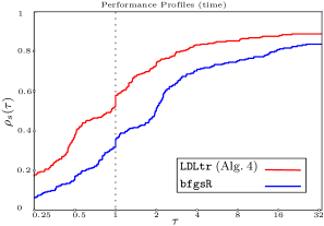
Figure 2: Computation-time extended performance profiles for Algorithm 4 and a strong Wolfe line-search BFGS algorithm on 252 CUTEst unconstrained problems with $n\leq 5000$ variables.

The profiles indicate that $\mathtt{LDLtr}$ required less overall cpu time than $\mathtt{bfgsR}$. The main reason for this appears to be the updating strategy of an $LDL^{\mskip 1.0mu\mathrm{\scriptstyle T}}$ factorization, which is implemented by updating the inverse factorization. Algorithm 4 ($\mathtt{LDLtr}$) is based on a modification of Algorithm C1 of Gill, Golub, Murray & Saunders [26], while $\mathtt{bfgsR}$ updates the Cholesky factors of $B_{k}$ using the method of Dennis & Schnabel [18].

In a second experiment $\mathtt{LDLtr}$ was compared to an implementation of the Moré-Sorensen (MS) trust-region algorithm ([40]). The MS algorithm is considered to be very robust, but requires $O(n^{3})$ flops per iteration. Therefore, the problem dimension is limited to $n\leq 1000$. (Note that $\mathtt{LDLtr}$ is applicable to larger problems, but MS is not.) The resulting test-set consisted of 161 problems. Many of the problems are relatively small, and any computational advantages in terms of time are also small. Based on the results of Fig. 3, the proposed strategy with two phases (including a branching for small and large problems) is also effective when compared to the MS algorithm.

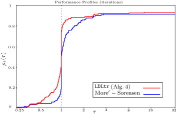
Figure 3: Extended iteration performance profiles for Algorithm 4 and the Moré-Sorensen method on 161 CUTEst unconstrained problems with $n\leq 1000$ variables.

6 Conclusions

An effective two-phase $LDL^{\mskip 1.0mu\mathrm{\scriptstyle T}}$ quasi-Newton trust-region algorithm has been formulated for smooth unconstrained optimization problems for which the second derivatives are not available. In the first phase, the $LDL^{\mskip 1.0mu\mathrm{\scriptstyle T}}$ factorization is used to compute an inexpensive estimate of the shift parameter associated with the optimality conditions for the two-norm trust-region subproblem. In the second phase, the factorization is used for a modified conjugate-gradient iteration that solves a system with the inverse approximate Hessian plus a shifted identity. Because the estimated shift parameter may be different from the optimal shift, a backtracking strategy on the shift is used to find the shift that gives the lowest function value. By updating the $LDL^{\mskip 1.0mu\mathrm{\scriptstyle T}}$ factorization with rank-one corrections and using two phases to generate a step, the algorithm has an overall complexity of $O(n^{2})$ flops. Numerical experiments show that the $LDL^{\mskip 1.0mu\mathrm{\scriptstyle T}}$ trust-region method is competitive with a strong Wolfe line-search quasi-Newton method on a subset of almost all unconstrained problems in the CUTEst test collection. The experiments indicate that the method inherits the robustness of the Moré-Sorensen trust-region method without the computational cost.

Appendix A Algorithm 2

Algorithm 2 is based on solving for $\sigma^{+}$ and $s^{+}$ in the optimality conditions (11), specifically so that $\|s^{+}\|_{2}=\Delta_{k}$. Note that, because of the first equation in (11), $s^{+}=s^{+}(\sigma^{+})$, i.e., the step $s^{+}$ is a function of $\sigma^{+}$. Instead of solving $\|s^{+}(\sigma^{+})\|_{2}=\Delta_{k}$ it is better numerically to solve the equivalent (secular) equation

$$\phi(\sigma^{+})=\frac{1}{\|s^{+}(\sigma^{+})\|_{2}}-\frac{1}{\Delta_{k}}=0.$$

This is a one-dimensional root finding problem in terms of $\sigma^{+}$, which can be solved with Newton’s method. Starting from an initial point $\sigma^{+}_{0}$, the iteration is

$$\sigma^{+}_{i+1}=\sigma^{+}_{i}-\frac{\phi(\sigma^{+}_{i})}{\phi^{\prime}(\sigma^{+}_{i})},\quad\quad i=0,1,\ldots.$$

If $q^{\scriptscriptstyle+}=q^{\scriptscriptstyle+}(\sigma)$ denotes the derivative $s^{+}{}^{\prime}=(s^{+}(\sigma))^{\prime}$, then $\phi^{\prime}(\sigma)$ is given by

$$\phi^{\prime}(\sigma)=\left(\frac{1}{\|s^{+}\|_{2}}-\frac{1}{\Delta_{k}}\right)^{\prime}=\left(\frac{1}{s^{+}{}^{\mskip 1.0mu\mathrm{\scriptstyle T}}s^{+}}\right)^{\prime}=-\frac{{{q^{\scriptscriptstyle+}}{}^{\mskip 1.0mu\mathrm{\scriptstyle T}}s^{+}}}{\|s^{+}\|_{2}^{3}}.$$

The quantity $q^{\scriptscriptstyle+}$ is computed from the equations

$$\left(L_{k}(D_{k}+\sigma E_{k})L_{k}^{\mskip 1.0mu\mathrm{\scriptstyle T}}s^{+}=-g_{k}\right){}^{\prime},\quad\;\;\text{i.e.,}\;\;L_{k}E_{k}L_{k}^{\mskip 1.0mu\mathrm{\scriptstyle T}}s^{+}+L_{k}(D_{k}+\sigma E_{k})L_{k}^{\mskip 1.0mu\mathrm{\scriptstyle T}}q^{\scriptscriptstyle+}=0,$$

which implies that

$$(D_{k}+\sigma E_{k})L_{k}^{\mskip 1.0mu\mathrm{\scriptstyle T}}q^{\scriptscriptstyle+}=-E_{k}L_{k}^{\mskip 1.0mu\mathrm{\scriptstyle T}}s^{+}.$$

The Newton correction at $\sigma$ is then

$$\frac{\phi(\sigma)}{\phi^{\prime}(\sigma)}=\frac{\phi}{\phi^{\prime}}=-\frac{\left(1/\|s^{+}\|_{2}-1/\Delta_{k}\right)}{s^{+}{}^{\mskip 1.0mu\mathrm{\scriptstyle T}}q^{\scriptscriptstyle+}/\|s^{+}\|_{2}^{3}}=-\frac{\|s^{+}\|_{2}^{2}}{s^{+}{}^{\mskip 1.0mu\mathrm{\scriptstyle T}}q^{\scriptscriptstyle+}}\Big{(}\frac{\Delta_{k}-\|s^{+}\|_{2}}{\Delta_{k}}\Big{)}.$$

It follows that at $\sigma=\sigma_{i}$, we have

$$\sigma_{i+1}=\sigma_{i}-\frac{\|s^{+}\|_{2}^{2}}{s^{+}{}^{\mskip 1.0mu\mathrm{\scriptstyle T}}q^{\scriptscriptstyle+}}\Big{(}\frac{\|s^{+}\|_{2}-\Delta_{k}}{\Delta_{k}}\Big{)},$$

which completes the derivation of the quantities used in Algorithm 2.

Appendix B Quasi-Newton $LDL^{\mskip 1.0mu\mathrm{\scriptstyle T}}$ Updates

In order to apply the $LDL^{\mskip 1.0mu\mathrm{\scriptstyle T}}$ updating strategy to (20) we reformulate the rank-2 update in (20) to conform to (4). Specifically, let

$$\beta_{1}=\frac{y_{k}^{\mskip 1.0mu\mathrm{\scriptstyle T}}s_{k}+y_{k}^{\mskip 1.0mu\mathrm{\scriptstyle T}}H_{k}y_{k}}{(y_{k}^{\mskip 1.0mu\mathrm{\scriptstyle T}}s_{k})^{2}},\qquad\beta_{2}=\frac{1}{y_{k}^{\mskip 1.0mu\mathrm{\scriptstyle T}}s_{k}},$$

and note that

$$\frac{(y_{k}^{\mskip 1.0mu\mathrm{\scriptstyle T}}s_{k}+y_{k}^{\mskip 1.0mu\mathrm{\scriptstyle T}}H_{k}y_{k})s_{k}}{(y_{k}^{\mskip 1.0mu\mathrm{\scriptstyle T}}s_{k})^{2}}\,s_{k}s_{k}^{\mskip 1.0mu\mathrm{\scriptstyle T}}-\frac{1}{y_{k}^{\mskip 1.0mu\mathrm{\scriptstyle T}}s_{k}}\big{(}H_{k}y_{k}s_{k}^{\mskip 1.0mu\mathrm{\scriptstyle T}}+s_{k}y_{k}^{\mskip 1.0mu\mathrm{\scriptstyle T}}H_{k}\big{)}\\ =\begin{bmatrix}s_{k}&H_{k}y_{k}\end{bmatrix}\begin{bmatrix}\phantom{-}\beta_{1}&-\beta_{2}\\ -\beta_{2}&\phantom{-}0\end{bmatrix}\begin{bmatrix}s_{k}&H_{k}y_{k}\end{bmatrix}^{\mskip 1.0mu\mathrm{\scriptstyle T}}.$$

The $2\times 2$ matrix can be factored as

$$\begin{bmatrix}\phantom{-}\beta_{1}&-\beta_{2}\\[5.0pt] -\beta_{2}&\phantom{-}0\end{bmatrix}=\begin{bmatrix}1&0\\[5.0pt] l_{21}&1\end{bmatrix}\begin{bmatrix}\alpha^{(1)}_{k}&\\ &\alpha^{(2)}_{k}\end{bmatrix}\begin{bmatrix}1&l_{21}\\[5.0pt] 0&1\end{bmatrix}.$$

where

$$\alpha^{(1)}_{k}=\beta_{1},\quad l_{21}=-\frac{\beta_{2}}{\beta_{1}},\quad\text{ and}\quad\alpha^{(2)}_{k}=-\frac{\beta^{2}_{2}}{\beta_{1}}.$$

If $a^{(1)}_{k}$ and $a^{(2)}_{k}$ denote the quantities

$$a^{(1)}_{k}=\begin{bmatrix}s_{k}&H_{k}y_{k}\end{bmatrix}\begin{bmatrix}1\\ l_{21}\end{bmatrix}=s_{k}+(y_{k}^{\mskip 1.0mu\mathrm{\scriptstyle T}}s_{k})\alpha^{(2)}_{k}H_{k}y_{k},\quad\text{and}\quad a^{(2)}_{k}=H_{k}y_{k},$$

then

$$\alpha^{(1)}_{k}a^{(1)}_{k}a^{(1)}_{k}{}^{\mskip 1.0mu\mathrm{\scriptstyle T}}+\alpha^{(2)}_{k}a^{(2)}_{k}a^{(2)}_{k}{}^{\mskip 1.0mu\mathrm{\scriptstyle T}}=\frac{(y_{k}^{\mskip 1.0mu\mathrm{\scriptstyle T}}s_{k}+y_{k}^{\mskip 1.0mu\mathrm{\scriptstyle T}}H_{k}y_{k})}{(y_{k}^{\mskip 1.0mu\mathrm{\scriptstyle T}}s_{k})^{2}}s_{k}s_{k}^{\mskip 1.0mu\mathrm{\scriptstyle T}}-\frac{1}{y_{k}^{\mskip 1.0mu\mathrm{\scriptstyle T}}s_{k}}\big{(}H_{k}y_{k}s_{k}^{\mskip 1.0mu\mathrm{\scriptstyle T}}+s_{k}y_{k}^{\mskip 1.0mu\mathrm{\scriptstyle T}}H_{k}\big{)}.$$

which are the updates used in (22) and (23).

References

- [1] Y. Achdou and O. Pironneau, 8. Calibration of Local Volatility with European Options, pp. 243–261, https://doi.org/10.1137/1.9780898717495.ch8, https://epubs.siam.org/doi/abs/10.1137/1.9780898717495.ch8.
- [2] I. Bongartz, A. R. Conn, N. I. M. Gould, and Ph. L. Toint, CUTE: Constrained and unconstrained testing environment, ACM Trans. Math. Software, 21 (1995), pp. 123–160.
- [3] L. Bottou, F. E. Curtis, and J. Nocedal, Optimization methods for large-scale machine learning, SIAM Review, 60 (2018), pp. 223–311, https://doi.org/10.1137/16M1080173, https://doi.org/10.1137/16M1080173.
- [4] C. G. Broyden, The convergence of a class of double-rank minimization algorithms 1. General considerations, IMA J. Applied Mathematics, 6 (1970), pp. 76–90, https://doi.org/10.1093/imamat/6.1.76, https://doi.org/10.1093/imamat/6.1.76, https://arxiv.org/abs/http://oup.prod.sis.lan/imamat/article-pdf/6/1/76/2233756/6-1-76.pdf.
- [5] C. G. Broyden, J. Dennis, J. E., and J. J. Moré, On the Local and Superlinear Convergence of Quasi-Newton Methods, IMA Journal of Applied Mathematics, 12 (1973), pp. 223–245, https://doi.org/10.1093/imamat/12.3.223, https://doi.org/10.1093/imamat/12.3.223, https://arxiv.org/abs/https://academic.oup.com/imamat/article-pdf/12/3/223/1917861/12-3-223.pdf.
- [6] J. J. Brust, Large-Scale Quasi-Newton Trust-Region Methods: High-Accuracy Solvers, Dense Initializations, and Extensions, PhD thesis, UC Merced, 2018.
- [7] J. J. Brust, J. B. Erway, and R. F. Marcia, On solving L-SR1 trust-region subproblems, Comput. Optim. Appl., 66 (2017), pp. 245–266.
- [8] J. J. Brust, R. F. Marcia, and C. G. Petra, Large-scale quasi-Newton trust-region methods with low-dimensional linear equality constraints, Comput. Optim. Appl., (2019), https://doi.org/10.1007/s10589-019-00127-4, https://doi.org/10.1007/s10589-019-00127-4.
- [9] J. J. Brust, R. F. Marcia, C. G. Petra, and M. A. Saunders, Large-scale optimization with linear equality constraints using reduced compact representation, SIAM Journal on Scientific Computing, 44 (2022), pp. A103–A127, https://doi.org/10.1137/21M1393819.
- [10] O. Burdakov, L. Gong, Y.-X. Yuan, and S. Zikrin, On efficiently combining limited memory and trust-region techniques, Mathematical Programming Computation, 9 (2016), pp. 101–134.
- [11] O. P. Burdakov, J. M. Martínez, and E. A. Pilotta, A limited-memory multipoint symmetric secant method for bound constrained optimization, Annals of Operations Research, 117 (2002), pp. 51–70.
- [12] R. Byrd, R. Schnabel, and G. Shultz, Approximate solution of the trust region problem by minimization over two-dimensional subspaces, Mathematical Programming, 40 (1988), pp. 247–263, https://doi.org/10.1007/BF01580735.
- [13] R. H. Byrd, D. C. Liu, and J. Nocedal, On the behavior of broyden’s class of quasi-newton methods, SIAM Journal on Optimization, 2 (1992), pp. 533–557, https://doi.org/10.1137/0802026, https://doi.org/10.1137/0802026.
- [14] R. H. Byrd, J. Nocedal, and R. A. Waltz, Knitro: An integrated package for nonlinear optimization, in Large-Scale Nonlinear Optimization, G. Di Pillo and M. Roma, eds., Springer US, Boston, MA, 2006, pp. 35–59, https://doi.org/10.1007/0-387-30065-1_4.
- [15] A. R. Conn, N. I. M. Gould, and Ph. L. Toint, Trust-Region Methods, Society for Industrial and Applied Mathematics (SIAM), Philadelphia, PA, 2000, https://doi.org/10.1137/1.9780898719857, https://epubs.siam.org/doi/abs/10.1137/1.9780898719857, https://arxiv.org/abs/https://epubs.siam.org/doi/pdf/10.1137/1.9780898719857.
- [16] Y.-H. Dai, Convergence properties of the BFGS algorithm, SIAM Journal on Optimization, 13 (2002), pp. 693–701, https://doi.org/10.1137/S1052623401383455.
- [17] J. E. Dennis, Jr. and J. J. Moré, Quasi-newton methods, motivation and theory, SIAM Review, 19 (1977), pp. 46–89, https://doi.org/10.1137/1019005, https://doi.org/10.1137/1019005.
- [18] J. E. Dennis, Jr. and R. B. Schnabel, A new derivation of symmetric positive definite secant updates, in Nonlinear Programming, 4 (Proc. Sympos., Special Interest Group on Math. Programming, Univ. Wisconsin, Madison, Wis., 1980), Academic Press, New York, 1981, pp. 167–199.
- [19] E. Dolan and J. Moré, Benchmarking optimization software with performance profiles, Math. Program., 91 (2002), pp. 201–213.
- [20] J. B. Erway, P. E. Gill, and J. D. Griffin, Iterative methods for finding a trust-region step, SIAM Journal on Optimization, 20 (2009), pp. 1110–1131, https://doi.org/10.1137/070708494.
- [21] R. Fletcher, A new approach to variable metric algorithms, The Computer Journal, 13 (1970), pp. 317–322, https://doi.org/10.1093/comjnl/13.3.317, https://doi.org/10.1093/comjnl/13.3.317, https://arxiv.org/abs/http://oup.prod.sis.lan/comjnl/article-pdf/13/3/317/988678/130317.pdf.
- [22] R. Fletcher, A model algorithm for composite nondifferentiable optimization problems, Math. Programming Stud., 17 (1982), pp. 67–76. Nondifferential and variational techniques in optimization (Lexington, Ky., 1980).
- [23] R. Fletcher and M. J. D. Powell, On the modification of ldlt factorizations, Math. Comp., 28 (1974), pp. 1067–1087.
- [24] D. M. Gay, Computing optimal locally constrained steps, SIAM J. Sci. Statist. Comput., 2 (1981), pp. 186–197.
- [25] M. E. Gertz, A quasi-newton trust-region method, Math. Program., Ser. A (2004), pp. 447–470, https://doi.org/10.1007/s10107-004-0511-1, https://arxiv.org/abs/https://doi.org/10.1007/s10107-004-0511-1.
- [26] P. E. Gill, G. H. Golub, W. Murray, and M. A. Saunders, Methods for modifying matrix factorizations, Mathematics of Computation, 28 (1974), pp. 505–535, http://www.jstor.org/stable/2005923 (accessed 2023-08-15).
- [27] P. E. Gill and W. Murray, Quasi-Newton Methods for Unconstrained Optimization, IMA Journal of Applied Mathematics, 9 (1972), pp. 91–108, https://doi.org/10.1093/imamat/9.1.91, https://doi.org/10.1093/imamat/9.1.91, https://arxiv.org/abs/https://academic.oup.com/imamat/article-pdf/9/1/91/2092553/9-1-91.pdf.
- [28] P. E. Gill, W. Murray, and M. A. Saunders, Snopt: An sqp algorithm for large-scale constrained optimization, SIAM Review, 47 (2005), pp. 99–131, https://doi.org/10.1137/S0036144504446096, https://doi.org/10.1137/S0036144504446096.
- [29] P. E. Gill and J. H. Runnoe, On recent developments in BFGS methods for unconstrained optimization, Center for Computational Mathematics Report CCoM 22-04, Department of Mathematics, University of California, San Diego, La Jolla, CA, 2022.
- [30] D. Goldfarb, A family of variable-metric methods derived by variational means, Math. Comp., 24 (1970), pp. 23–26, https://doi.org/10.1090/S0025-5718-1970-0258249-6, https://doi.org/10.1090/S0025-5718-1970-0258249-6.
- [31] G. H. Golub and C. F. Van Loan, Matrix Computations, Johns Hopkins Studies in the Mathematical Sciences, The Johns Hopkins University Press, Baltimore, fourth ed., 2013.
- [32] N. I. M. Gould, S. Lucidi, M. Roma, and P. L. Toint, Solving the trust-region subproblem using the lanczos method, SIAM Journal on Optimization, 9 (1999), pp. 504–525, https://doi.org/10.1137/S1052623497322735.
- [33] N. I. M. Gould, D. Orban, and P. L. Toint, CUTEr and SifDec: A constrained and unconstrained testing environment, revisited, ACM Trans. Math. Softw., 29 (2003), pp. 373–394.
- [34] W. W. Hager, Minimizing a quadratic over a sphere, SIAM Journal on Optimization, 12 (2001), pp. 188–208, https://doi.org/10.1137/S1052623499356071.
- [35] M. D. Hebden, An algorithm for minimization using exact second derivatives, Tech. Report T.P. 515, Atomic Energy Research Establishment, Harwell, England, 1973.
- [36] M. R. Hestenes and E. Stiefel, Methods of conjugate gradients for solving linear systems, J. Research Nat. Bur. Standards, 49 (1952), pp. 409–436.
- [37] L. Luksan, Efficient trust region method for nonlinear least squares, Kybernetika, 32 (1996), pp. 105–120.
- [38] A. Mahajan, S. Leyffer, and C. Kirches, Solving mixed-integer nonlinear programs by qp diving, Technical Report ANL/MCS-P2071-0312, Mathematics and Computer Science Division, Argonne National Laboratory, Lemont, IL, 2012.
- [39] Matlab optimization toolbox, 2023. The MathWorks, Natick, MA, USA.
- [40] J. J. Moré and D. C. Sorensen, Computing a trust region step, SIAM J. Sci. Statist. Comput., 4 (1983), pp. 553–572.
- [41] J. J. Moré and D. J. Thuente, Line search algorithms with guaranteed sufficient decrease, ACM Trans. Math. Softw., 20 (1994), p. 286–307, https://doi.org/10.1145/192115.192132.
- [42] M. J. D. Powell, A hybrid method for nonlinear equations, in Numerical Methods for Nonlinear Algebraic Equations, P. Rabinowitz, ed., Gordon and Breach, 1970.
- [43] M. J. D. Powell, A new algorithm for unconstrained optimization, in Nonlinear Programming, J. Rosen, O. Mangasarian, and K. Ritter, eds., Academic Press, 1970, pp. 31–65, https://doi.org/https://doi.org/10.1016/B978-0-12-597050-1.50006-3.
- [44] P. Schwerdtner and M. Voigt, Sobmor: Structured optimization-based model order reduction, SIAM Journal on Scientific Computing, 45 (2023), pp. A502–A529, https://doi.org/10.1137/20M1380235, https://doi.org/10.1137/20M1380235.
- [45] D. F. Shanno, Conditioning of quasi-Newton methods for function minimization, Math. Comp., 24 (1970), pp. 647–656, https://doi.org/10.1090/S0025-5718-1970-0274029-X, https://doi.org/10.1090/S0025-5718-1970-0274029-X.
- [46] D. C. Sorensen, Newton’s method with a model trust region modification, SIAM J. Numer. Anal., 19 (1982), pp. 409–426.
- [47] T. Steihaug, The conjugate gradient method and trust regions in large scale optimization, SIAM J. Numer. Anal., 20 (1983), pp. 626–637.
- [48] P. L. Toint, Towards an efficient sparsity exploiting Newton method for minimization, in Sparse Matrices and Their Uses, I. S. Duff, ed., London and New York, 1981, Academic Press, pp. 57–88.
- [49] A. Wächter and L. T. Biegler, On the implementation of an interior-point filter line-search algorithm for large-scale nonlinear programming, Math. Program., 106 (2006), pp. 25–57.