Dozerformer: Sequence Adaptive Sparse Transformer for Multivariate Time Series Forecasting

Abstract

Transformers have achieved remarkable performance in multivariate time series(MTS) forecasting due to their capability to capture long-term dependencies. However, the canonical attention mechanism has two key limitations: (1) its quadratic time complexity limits the sequence length, and (2) it generates future values from the entire historical sequence. To address this, we propose a Dozer Attention mechanism consisting of three sparse components: (1) Local, each query exclusively attends to keys within a localized window of neighboring time steps. (2) Stride, enables each query to attend to keys at predefined intervals. (3) Vary, allows queries to selectively attend to keys from a subset of the historical sequence. Notably, the size of this subset dynamically expands as forecasting horizons extend. Those three components are designed to capture essential attributes of MTS data, including locality, seasonality, and global temporal dependencies. Additionally, we present the Dozerformer Framework, incorporating the Dozer Attention mechanism for the MTS forecasting task. We evaluated the proposed Dozerformer framework with recent state-of-the-art methods on nine benchmark datasets and confirmed its superior performance. The code will be released after the manuscript is accepted.

1 Introduction

Multivariate time series (MTS) forecasting endeavors to adeptly model the dynamic evolution of multiple variables over time from their historical records, thereby facilitating the accurate prediction of future values. This task holds significant importance in various applications Petropoulos et al. (2022). The advent of deep learning has significantly advanced MTS forecasting, various methods are proposed based on Recurrent Neural Networks (RNN) Lai et al. (2018), Convolutional Neural Networks (CNN) Shih et al. (2019); Wang et al. (2023). In recent years, the Transformer has demonstrated remarkable efficacy in MTS forecasting. This notable performance can be attributed to its inherent capacity to effectively capture global temporal dependencies across the entirety of the historical sequence. The Transformer is initially proposed for natural language processing(NLP) Vaswani et al. (2017) tasks, with its primary objective of extracting information from words within sentences. It achieved great success in the NLP field and swiftly extended its impact in computer vision Dosovitskiy et al. (2021) and time series analysis Wen et al. (2023). The critical challenge for applying transformers in MTS forecasting is to modify the attention mechanism based on the characteristics of time series data. Informer Zhou et al. (2021), Autoformer Wu et al. (2021), FEDformer Zhou et al. (2022), and Crossformer Zhang & Yan (2023) modified the canonical full attention mechanism to improve its efficiency and achieved promising results in MTS forecasting. Dlinear Zeng et al. (2023) challenges the effectiveness of the transformer by proposing a straightforward linear layer to infer historical records to predictions directly and outperforming aforementioned Transformer-based methods on benchmark datasets.

Nevertheless, these methods generate predictions for all future time steps from the entire historical sequence. Thus, they ignored that the look-back window of historical time steps is critical in generating accurate predictions. For example, predicting the value at horizon 1 using the entire historical sequence is suboptimal and inefficient. Figure 1(b) shows the full attention mechanism generating predictions, it generates predictions for all $O$ future time steps from the entire historical sequence of length $I$. They also ignored the characteristics of MTS data, like locality and seasonality. Figure 1(a) shows the heatmap of correlation among 168 time steps of four datasets that indicate clear locality and seasonality. An attention mechanism should only utilize those time steps that have a high correlation with the prediction target.

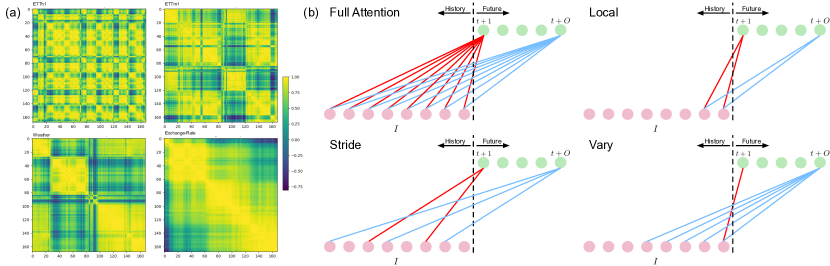
Figure 1: (a) The heatmap illustrates the correlation among 168 time steps for the ETTh1, ETTm1, Weather, and Exchange-Rate datasets. (b) Full Attention: Generates predictions using the entire historical sequence. Local Component: Utilizes time steps within a specified window. Stride Component: Utilizes time steps at fixed intervals from the target. Vary Component: Adaptively uses historical time steps as the forecasting horizon increases.

To address those issues, we propose Dozerformer, a novel framework that incorporates an innovative attention mechanism comprising three key components: Local, Stride, and Vary. Figure 1(b) illustrates the concept of the Local, Stride, and Vary components. They leverage historical time steps based on the distinctive characteristics of MTS data. The Local component exclusively considers time steps within a window determined by the target time step. The Stride component selectively employs time steps that are at fixed intervals from the target time step. Lastly, the Vary component dynamically adjusts its use of historical time steps according to the forecasting horizon—employing a shorter historical sequence for shorter horizons and a longer one for longer horizons. The contributions of our work are summarized as follows:

• We introduce a sequence-adaptive sparse Dozer Attention mechanism composed of three components: Local, Stride, and Vary. Each component aims to capture temporal dependencies from a select number of effective historical time steps. Notably, the Vary component dynamically expands its utilization of historical time steps as the forecasting horizons extend.

• We propose the Dozerformer framework for MTS forecasting, incorporating the Dozer Attention mechanism designed to model and predict the seasonal components within MTS data.

• The experimental results on nine benchmark datasets showcase Dozerformer’s superior performance in terms of both accuracy and efficiency when compared to recent state-of-the-art methods.

2 Related Work

2.1 MTS Forecasting

MTS forecasting involves predicting values ($X_{pred}\in\mathbb{R}^{O\times D}$) of $D$ variables for future $O$ time steps, given their historical records within the look-back window ($X\in\mathbb{R}^{I\times D}$) spanning $I$ time steps. Deep learning has significantly advanced MTS forecasting. LSTNet Lai et al. (2018) employs CNN and RNN to capture both short-term and long-term temporal dependencies. TPA-LSTM Shih et al. (2019) introduces a temporal pattern attention mechanism to weight hidden states across historical time steps. Graph WaveNet Wu et al. (2019) pioneers the use of Graph Neural Networks (GNN) for MTS forecasting, jointly training an adjacency matrix to model spatial dependencies. MTGNN Wu et al. (2020) is the first GNN-based method for generic MTS forecasting. It utilizes GNN to model correlations among multiple variables and CNN with different filter sizes to model multi-scale temporal dependencies. Transformers Wen et al. (2023) gained popularity in MTS forecasting due to their capacity to capture long-term temporal dependencies. The attention mechanism enables modeling temporal dependencies across all historical time steps. While CNN needs to be stacked, RNN needs to iteratively go through all time steps, and GNN is vulnerable to the adjacency matrix which indicates the correlation between variables. MICN Wang et al. (2023) replaces self-attention with a CNN-based local-global structure to model temporal dependencies across scales efficiently. Dlinear Zeng et al. (2023) challenges transformer effectiveness with a simple linear layer, achieving state-of-the-art performance. PatchTST Nie et al. (2023) highlights the significance of transformers in modeling temporal dependencies at sub-series resolution, independently of variables. In summary, transformers have pushed the boundaries of MTS forecasting.

2.2 Sparse Self Attentions

Transformers have achieved significant achievements in various domains, including NLP Vaswani et al. (2017), computer vision Dosovitskiy et al. (2021), and time series analysis Wen et al. (2023). However, their quadratic computational complexity limits input sequence length. Recent studies have tackled this issue by introducing modifications to the full attention mechanism. Longformer Beltagy et al. (2020) introduces a sparse attention mechanism, where each query is restricted to attending only to keys within a defined window or dilated window, except for global tokens, which interact with the entire sequence. Similarly, BigBird Zaheer et al. (2020) proposes a sparse attention mechanism consisting of Random, Local, and Global components. The Random component limits each query to attend a fixed number of randomly selected keys. The Local component allows each query to attend keys of nearby neighbors. The Global component selects a fixed number of input tokens to participate in the query-key production process for the entire sequence. In contrast to NLP, where input consists of word sequences, and computer vision Khan et al. (2022), where image patches are used, time series tasks involve historical records at multiple time steps. To effectively capture time series data’s seasonality, having a sufficient historical record length is crucial. For instance, capturing weekly seasonality in MTS data sampled every 10 minutes necessitates approximately $6\times 24\times 7$ time steps. Consequently, applying the Transformer architecture to time series data is impeded by its quadratic computational complexity. To address this challenge, various methods have been proposed. Informer Zhou et al. (2021) introduces a ProbSparse attention mechanism, allowing each key to attend to a limited number of queries. This modification achieves $\mathcal{O}(I\log I)$ complexity in both computational and memory usage. Autoformer Wu et al. (2021) proposes an Auto-Correlation mechanism designed to model period-based temporal dependencies. It achieves $\mathcal{O}(I\log I)$ complexity by selecting only the top $logI$ query-key pairs. FEDformer Zhou et al. (2022) introduces frequency-enhanced blocks, including Fourier and Wavelet components, to transform queries, keys, and values into the frequency domain. The attention mechanism computes a fixed number of randomly selected frequency components from queries, keys, and values, resulting in linear complexity. Both Crossformer Zhang & Yan (2023) and PatchTST Nie et al. (2023) propose patching mechanisms that partition time series data into patches spanning multiple time steps, effectively reducing the total length of the historical sequence.

3 Method

In this section, we present the Dozerformer method, which incorporates the Dozer attention mechanism. Section 3.1 introduces the Dozerformer framework, which includes a transformer encoder-decoder pair and a linear layer designed for forecasting seasonal and trend components of MTS data, respectively. Section 3.2 provides a comprehensive description of the proposed Dozer attention mechanism, with its primary concept centered around the elimination of query-key pairs between input and output time steps that do not contribute to accuracy.

3.1 Framework

The MTS forecasting task aims to infer values of $D$ variables for future $O$ time steps $X\in\mathbb{R}^{O\times D}$ from their historical records $X\in\mathbb{R}^{I\times D}$. Figure 2 illustrates the overall framework of Dozerformer. Initially, it decomposes the MTS data into seasonal and trend components, following previous methods Wu et al. (2021); Zhou et al. (2022); Zeng et al. (2023). Subsequently, the transformer and linear models are employed to generate forecasts for the seasonal component $\mathbf{X}_{s}\in\mathbb{R}^{I\times D}$ and the trend component $\mathbf{X}_{t}\in\mathbb{R}^{I\times D}$, respectively.

The dimension invariant (DI) embed Zhang et al. (2023) transforms raw single-channel MTS data into multi-channel feature maps while preserving both the time step and variable dimensions. It further partitions the MTS data into multiple patches along the time step dimension, resulting in patched MTS embeddings denoted as $X_{enc}\in\mathbb{R}^{c\times N_{enc}\times p\times D}$. Here, $c$ represents the number of feature maps, $N_{enc}=\lceil I/p\rceil$ indicates the number of patches for the encoder, and $p$ represents the patch size. Similarly, the decoder’s input, denoted as $X_{dec}\in\mathbb{R}^{c\times N_{dec}\times p\times D}$ (not shown in Figure 2), is derived from $L$ historical time steps and $O$ zero padding. In this context, $N_{dec}=\lceil(L+O)/p\rceil$ indicates the number of patches for the decoder. The transformer model is designed to capture temporal dependencies at multiple time step resolutions (sub-series level). While the transformer encoder and decoder adhere to the canonical transformer architecture Vaswani et al. (2017), they employ the proposed Dozer attention mechanism in place of the canonical full attention. A $1\times 1$ CNN is employed to generate seasonal component predictions based on the learned latent representations from the transformer.

To predict the trend component, we employ a linear layer for the direct inference of trend forecasts from historical trend components. Subsequently, the forecasts for the seasonal and trend components are aggregated by summation to obtain the final predictions denoted as $\mathbf{X}_{pred}\in\mathbb{R}^{O\times D}$.

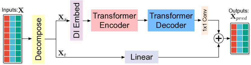
Figure 2: The architecture of our proposed Dozerformer framework.

3.2 dozer attention

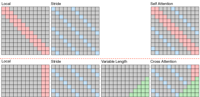
Figure 3: The illustration of the Dozer attention mechanism. Upper: The self-attention consists of Local and Stride. Lower: The cross attention consists of Local, Stride, and Vary.

The canonical scaled dot-product attention is as follows:

$$\begin{split}Q,K,V&=\operatorname{Linear}\left(\mathbf{X}_{enc}\right)\\ \operatorname{Attention}\left(Q,K,V\right)&=\operatorname{Softmax}\left(QK^{T}/\sqrt{d_{k}}\right)V\end{split}$$ (1)

where the $Q$, $K$, and $V$ represent the query, keys, and values obtained through embedding from the input sequence of the $d$-th series, denoted as $\mathbf{X}{enc}^{d}\in\mathbb{R}^{c\times N{enc}\times p}$. It’s noteworthy that we flatten both the feature map and patch size dimensions of $\mathbf{X}{enc}^{d}$, resulting in $\mathbf{X}{enc}^{d}\in\mathbb{R}^{N_{enc}\times(c\times p)}$, representing the latent representations of patches with a size of $p_{k}$. The canonical transformer exhibits two key limitations: firstly, its encoder’s self-attention is afflicted by quadratic computational time complexity, thereby restricting the length of $N_{enc}$; secondly, its decoder’s cross-attention employs the entire sequence to forecast all future time steps, entailing unnecessary computation for ineffective historical time steps. To overcome these issues, we propose a Dozer attention mechanism, comprising three components: Local, Stride, and Vary.

In Figure 3, we illustrate the sparse attention matrices of Local, Stride, and Vary components employed in the proposed Dozer attention mechanism. Squares shaded in gray signify zeros, indicating areas where the computation of the query-key product is redundant and thus omitted. These areas represent saved computations compared to full attention. The pink-colored squares correspond to the Local component, signifying that each query exclusively calculates the product with keys that fall within a specified window. Blue squares denote the Stride component, where each query selectively attends to keys that are positioned at fixed intervals. The green squares represent the Vary component, where queries dynamically adapt their attention to historical sequences of varying lengths based on the forecasting horizons. As a result, the Dozer attention mechanism exclusively computes the query-key pairs indicated by colored (pink, blue, and green) squares while efficiently eliminating the computation of gray query-key pairs.

3.2.1 Local

The MTS data comprises variables that change continuously and exhibit locality, with nearby values in the time dimension displaying higher correlations than those at greater temporal distances. This characteristic is evident in Figure 3, which illustrates the strong locality within MTS data. Building upon this observation, we introduce the Local component, a key feature of our approach. In the Local component, each query selectively attends to keys that reside within a specified time window along the temporal dimension. Equation 2 defines the Local component as follows:

$$\begin{split}A^{self}_{i,j}&=\begin{cases}q_{i}*k_{j},\qquad&\text{if $j\in\{|i-j|<=\lfloor w/2\rfloor\}$}\\ 0,\qquad&\text{otherwise}\\ \end{cases}\\ A^{cross}_{i,j}&=\begin{cases}q_{i}*k_{j},\qquad&\text{if $j\in\{0<=t-j<=\lfloor w/2\rfloor\}$}\\ 0,\qquad&\text{otherwise}\end{cases}\\ \end{split}$$ (2)

In the case of self-attention, the Local component enables each query to selectively attend to a specific set of keys that fall within a defined time window. Specifically, each query in self-attention attends to $\lfloor w/2\rfloor+1$ keys, with $\lfloor w/2\rfloor$ keys representing the neighboring time steps on each side of the query. For cross-attention, the concept of locality differs since future time steps cannot be utilized during forecasting. Instead, the locality is derived from the last $\lfloor w/2\rfloor+1$ time steps, situated at the end of the sequence. These steps encompass the most recent time points up to the moment of forecasting, denoted as time $t$.

3.2.2 Stride

Seasonality is a key characteristic of time series data, and to capture this attribute effectively, we introduce the Stride component. In this component, each query selectively attends to keys positioned at fixed intervals in the temporal dimension. To illustrate this concept, let’s consider a query at time step $t$, denoted as $q_{t}$, and assume that the time series data exhibits a seasonality pattern with a period ($interval$). Equation 3 defines the Stride component as follows:

$$A_{i,j}=\begin{cases}q_{i}*k_{j}\qquad&\text{if $j\in\{|i-j|\%interval==0\}$}\\ 0,\qquad&\text{otherwise}\end{cases}$$ (3)

In self-attention, the Stride component initiates by computing the product between the query $q_{t}$ and the key at the same time step, denoted as $k_{t}$. It then progressively expands its attention to keys positioned at a temporal distance of $interval$ time steps from $t$, encompassing keys like $k_{t-interval}$, $k_{t+interval}$, and so forth, until it spans the entire sequence range. For cross-attention, the Stride component identifies time steps within the input sequence $X_{I}$ that are separated by multiples of $interval$ time steps, aligning with the seasonality pattern. Hence, the Stride component consistently computes attention scores (query-key products) using these selected keys from the Encoder’s $I$ input time steps, yielding a total of $s=\lfloor I/interval\rfloor$ query-key pairs.

3.2.3 Vary

In the context of MTS forecasting scenarios employing the canonical attention mechanism, predictions for all future time steps are computed through a weighted sum encompassing the entirety of the historical sequence. Regardless of the forecasting horizon, this canonical cross-attention mechanism diligently computes all possible query-key pairs. However, it is important to recognize that harnessing information from the entire historical sequence does not necessarily improve forecasting accuracy, especially in the case of time series data characterized by evolving distributions, as exemplified by stock prices.

To tackle this challenge, we propose the Vary component, which dynamically expands the historical time steps considered as the forecasting horizon extends. We define the initial length of the historical sequence utilized as $v$. When forecasting a single time step into the future (horizon of 1), the Vary component exclusively utilizes $v$ time steps from the sequence. As the forecasting horizon increases gradually by 1, the history length used also increments by 1, starting from the vary window $v$ until it reaches the maximum input length. Equation 4 defines the Vary component as follows:

$$A^{cross}_{i,j}=\begin{cases}q_{i}*k_{j},\qquad&\text{if $j\in\{t-1,t-2,\cdots,t-v+i-t\}$ and $i>t$}\\ 0,\qquad&\text{otherwise}\end{cases}$$ (4)

4 Experiments

4.1 Experimental settings

Datasets. We conduct experiments on 9 public benchmarks Wu et al. (2021), including 4 ETT datasets(ETTh1, ETTh2, ETTm1, ETTm2), Traffic, Electricity, Weather, Exchange-Rate, and ILI. These are widely used real-world MTS datasets with different characteristics.

Comparison methods. We compare our Dozerformer with seven transformer-based methods (Informer Zhou et al. (2021), Autoformer Wu et al. (2021), FEDformer Zhou et al. (2022), Pyraformer Liu et al. (2022), Crossformer Zhang & Yan (2023), PatchTST Nie et al. (2023)), CNN-based method MICN Wang et al. (2023), and Linear method Dlinear Zeng et al. (2023).

Evaluation metrics. We utilize Mean Squared Error (MSE) and Mean Absolute Error (MAE) as the evaluation metrics to compare the forecasting accuracy.

Training details. We implemented the proposed Dozerformer in Pytorch and trained with Adam optimizer ($\beta_{1}=0.9$ and $\beta_{2}=0.99$). The initial learning rate is selected from $\{5e-5,1e-4,5e-4,1e-3\}$ via grid search and updated using the Cosine Annealing scheme. The transformer encoder layer is set to 2 and the decoder layer is set to 1. We select the look-back window size of historical time steps utilized from $\{96,192,336,720\}$ via grid search except for the ILI dataset which is set to $120$. The patch size is selected from $\{24,48,96\}$ via grid search. The main results are repeated six times using seeds $1,2022,2023,2024,2025$, and $2026$. The ablations study and parameter sensitivity results are obtained from random seed $1$.

4.2 Main Results

Table 1 presents a quantitative comparison between the proposed Dozerformer and baseline methods across nine benchmarks using MSE and MAE, where the bolded and underlined case (dataset, horizon, and metric) represent the best and second-best results, respectively. The Dozerformer achieved superior performance than state-of-the-art baseline methods by performing the best in 48 cases and second-best in 22 cases. Compared to state-of-the-art baseline methods, Dozerformer achieved reductions in MSE: 0.4% lower than PatchTST Nie et al. (2023), 8.3% lower than Dlinear Zeng et al. (2023), 20.6% lower than MICN Wang et al. (2023), and a substantial 40.6% lower than Crossformer Zhang & Yan (2023). While PatchTST came closest to our method in performance, it utilizes full attention, making it less efficient in terms of computational complexity and memory usage. We conclude that Dozerformer outperforms recent state-of-the-art baseline methods in terms of accuracy.

Table 1: Comparison of quantitative results (MSE&MAE) on nine datasets for forecasting horizons $O\in\{96,192,336,720\}$ (For ILI, $O\in\{24,36,48,60\}$). Bold and underlined highlight the best and second-best results, respectively.

Methods		Dozerformer	PatchTST	DLinear	Crossformer	MICN	Pyraformer	FEDformer	Autoformer	Informer
Metric		MSE  MAE	MSE  MAE	MSE  MAE	MSE  MAE	MSE  MAE	MSE  MAE	MSE  MAE	MSE  MAE	MSE  MAE
ETTh1	96	0.363  0.386	0.370  0.400	0.375  0.399	0.431  0.458	0.421  0.431	0.664  0.612	0.376  0.419	0.449  0.459	0.865  0.713
	192	0.405  0.413	0.413  0.429	0.405  0.416	0.420  0.448	0.474  0.487	0.790  0.681	0.420  0.448	0.500  0.482	1.008  0.792
	336	0.432  0.428	0.422  0.440	0.439  0.443	0.440  0.461	0.569  0.551	0.891  0.738	0.459  0.465	0.521  0.496	1.107  0.809
	720	0.453  0.459	0.447  0.468	0.472  0.490	0.519  0.524	0.770  0.672	0.963  0.782	0.506  0.507	0.514  0.512	1.181  0.865
ETTh2	96	0.273  0.329	0.274  0.337	0.289  0.353	1.177  0.757	0.299  0.364	0.645  0.597	0.358  0.397	0.358  0.397	3.755  1.525
	168	0.341  0.374	0.341  0.382	0.383  0.418	1.206  0.796	0.441  0.454	0.788  0.683	0.429  0.439	0.456  0.452	5.602  1.931
	336	0.364  0.400	0.329  0.384	0.448  0.465	1.452  0.883	0.654  0.567	0.907  0.747	0.496  0.487	0.482  0.486	4.721  1.835
	720	0.394  0.432	0.379  0.422	0.605  0.551	2.040  1.121	0.956  0.716	0.963  0.783	0.463  0.474	0.515  0.511	3.647  1.625
ETTm1	96	0.290  0.332	0.293  0.346	0.299  0.343	0.320  0.373	0.316  0.362	0.543  0.510	0.379  0.419	0.505  0.475	0.672  0.571
	192	0.328  0.356	0.333  0.370	0.335  0.365	0.400  0.432	0.363  0.390	0.557  0.537	0.426  0.441	0.553  0.496	0.795  0.669
	336	0.360  0.375	0.369  0.392	0.369  0.386	0.408  0.428	0.408  0.426	0.754  0.655	0.445  0.459	0.621  0.537	1.212  0.871
	720	0.416  0.410	0.416  0.420	0.425  0.421	0.582  0.537	0.481  0.476	0.908  0.724	0.543  0.490	0.671  0.561	1.166  0.823
ETTm2	96	0.164  0.248	0.166  0.256	0.167  0.260	0.444  0.463	0.179  0.275	0.435  0.507	0.203  0.287	0.255  0.339	0.365  0.453
	192	0.217  0.285	0.223  0.296	0.224  0.303	0.833  0.657	0.307  0.376	0.730  0.673	0.269  0.328	0.281  0.340	0.533  0.563
	336	0.270  0.323	0.274  0.329	0.281  0.342	0.766  0.620	0.325  0.388	1.201  0.845	0.325  0.366	0.339  0.372	1.363  0.887
	720	0.354  0.378	0.362  0.385	0.397  0.421	0.959  0.752	0.502  0.490	3.625  1.451	0.421  0.415	0.433  0.432	3.379  1.338
Traffic	96	0.380  0.241	0.360  0.249	0.410  0.282	0.538  0.300	0.519  0.309	0.867  0.468	0.587  0.366	0.613  0.388	0.719  0.391
	192	0.386  0.244	0.379  0.256	0.423  0.287	0.515  0.288	0.537  0.315	0.869  0.467	0.604  0.373	0.616  0.382	0.696  0.379
	336	0.415  0.255	0.392  0.264	0.436  0.296	0.530  0.300	0.534  0.313	0.881  0.469	0.621  0.383	0.622  0.337	0.777  0.420
	720	0.471  0.281	0.432  0.286	0.466  0.315	0.573  0.313	0.577  0.325	0.896  0.473	0.626  0.382	0.660  0.408	0.864  0.472
Electricity	96	0.127  0.219	0.129  0.222	0.140  0.237	0.141  0.240	0.164  0.269	0.386  0.449	0.193  0.308	0.201  0.317	0.274  0.368
	192	0.142  0.234	0.147  0.240	0.153  0.249	0.166  0.265	0.177  0.177	0.378  0.443	0.201  0.315	0.222  0.334	0.296  0.386
	336	0.158  0.253	0.163  0.259	0.169  0.267	0.323  0.369	0.193  0.304	0.376  0.443	0.214  0.329	0.231  0.338	0.300  0.394
	720	0.196  0.291	0.197  0.290	0.203  0.301	0.404  0.423	0.212  0.321	0.376  0.445	0.246  0.355	0.254  0.361	0.373  0.439
Weather	96	0.145  0.190	0.149  0.198	0.176  0.237	0.158  0.231	0.161  0.229	0.622  0.556	0.217  0.296	0.266  0.336	0.300  0.384
	192	0.190  0.234	0.194  0.241	0.220  0.282	0.194  0.262	0.220  0.281	0.739  0.624	0.276  0.336	0.307  0.367	0.598  0.544
	336	0.237  0.271	0.245  0.282	0.265  0.319	0.495  0.515	0.278  0.331	1.004  0.753	0.339  0.380	0.359  0.395	0.578  0.523
	720	0.308  0.321	0.314  0.334	0.323  0.362	0.526  0.542	0.311  0.356	1.420  0.934	0.403  0.428	0.419  0.428	1.059  0.741
Exchange	96	0.086  0.210	0.896  0.209	0.081  0.203	0.323  0.425	0.102  0.235	1.748  1.105	0.148  0.278	0.197  0.323	0.847  0.752
	192	0.167  0.293	0.187  0.308	0.157  0.293	0.448  0.506	0.172  0.316	1.874  1.151	0.271  0.380	0.300  0.369	1.204  0.895
	336	0.266  0.380	0.349  0.432	0.305  0.414	0.840  0.718	0.272  0.407	1.943  1.172	0.460  0.500	0.509  0.524	1.672  1.036
	720	0.600  0.590	0.900  0.715	0.643  0.601	1.416  0.959	0.714  0.658	2.085  1.206	1.195  0.841	1.447  0.941	2.478  1.310
ILI	24	1.656  0.863	1.319  0.754	2.215  1.081	3.041  1.186	2.684  1.112	7.394  2.012	3.228  1.260	3.483  1.287	5.764  1.677
	36	1.491  0.832	1.579  0.870	1.963  0.963	3.406  1.232	2.667  1.068	7.551  2.031	2.679  1.080	3.103  1.148	4.755  1.467
	48	1.597  0.854	1.553  0.815	2.130  1.024	3.459  1.221	2.558  1.052	7.662  2.057	2.622  1.078	2.669  1.085	4.763  1.469
	60	1.770  0.887	1.470  0.788	2.368  1.096	3.640  1.305	2.747  1.110	7.931  2.100	2.857  1.157	2.770  1.125	5.264  1.564

4.3 Computational Efficiency

We analyze the computational complexity of transformer-based methods and present it in Table 2. For self-attention, the proposed Dozer self-attention achieved linear computational complexity w.r.t $I$ with a coefficient $(w+s)/p$. $w$ and $s$ denote the keys that the query attends with respect to Local and Stride components, which are small numbers (e.g. $w\in\{1,3\}$ and $s\in\{2,3\}$). In contrast, $p$ corresponds to the size of time series patches and is set to a larger value (e.g., $p\in{24,48,96}$). We conclude that the coefficient $(w+s)/p$ is consistently smaller than $1$ under the experimental conditions, highlighting the superior computational complexity performance of Dozer self-attention.

To analyze the computational complexity of cross-attention, it’s essential to consider the specific design of the decoder for each method and analyze them individually. The Transformer calculates production between all $L+O$ queries and $I$ keys, with its complexity influenced by inputs for both the encoder and decoder. The Informer selects $log(L+O)$ queries and $I/2$ keys (time steps near $t$), resulting in $\mathcal{O}(log(L+O)I/2)$. Autoformer and FEDformer pad zeros to keys when $I$ is smaller than $L+O$ and only select the last $L+O$ keys when $I$ is greater than $L+O$. As a result, their cross-attention complexity is linear w.r.t $L+O$. The Crossformer decoder takes only $O$ zero paddings as input. Consequently, its cross-attention attends to $O/p$ queries and $I/p$ keys. It’s worth noting that Crossformer also applies full attention across the variable dimension, so its complexity is additionally influenced by the variable count $D$. PatchTST solely employs the transformer encoder, making cross-attention irrelevant in this context.

The Local and Stride components of Dozer cross-attention specifically address $(L+O)/p$ queries, calculating the product of each query with $w$ keys within the local window and $s$ keys positioned at fixed intervals from the query. Consequently, their computational complexity is linear with respect to $L+O$, characterized by the coefficient $(w+s)/p$. The Vary component’s complexity exhibits a quadratic relationship with respect to $O$, with a coefficient of $1/(2p^{2})$. This quadratic complexity is notably more efficient compared to linear complexity when $O<2p^{2}$ (e.g. 1152 when $p=24$). Additionally, the Vary component maintains linear complexity concerning $O$ when $v$ is greater than 1, although its coefficient $(v-1)/p$ should be significantly less than 1 for practical efficiency. Throughout all experiments, we consistently set $v$ to 1, rendering $(v-1)O/p$ negligible.

The memory complexity of the Dozer Attention is $\mathcal{O}((w+s)I/p)$ for self-attention and $\mathcal{O}((w+s)(L+O)/p+(O/p)^{2}/2+(v-1)O/p)$ for cross-attention. It’s worth noting that the analysis of Dozer Attention’s computational complexity is equally applicable to its memory complexity. In conclusion, the Local and Stride components excel in efficiency by attending queries to a limited number of keys. As for the Vary component, it proves to be more efficient than linear complexity in practical scenarios, with its complexity only influenced by forecasting horizons.

Table 2: Computational complexity of self-attention and cross-attention. The Encoder’s input historical sequence length is denoted $I$, and The decoder’s input historical sequence length and forecasting horizons are denoted as $L$ and $O$, respectively. $D$ indicates the variable dimension of MTS data. $p$ is the patch size.

Methods	Self-Attention	Cross-Attention
Transformer Vaswani et al. (2017)	$\mathcal{O}(I^{2})$	$\mathcal{O}((L+O)I)$
Informer Zhou et al. (2021)	$\mathcal{O}(IlogI)$	$\mathcal{O}(log(L+O)I/2)$
Autoformer Wu et al. (2021)	$\mathcal{O}(IlogI)$	$\mathcal{O}((L+O)log(L+O))$
Fedformer Zhou et al. (2022)	$\mathcal{O}(I)$	$\mathcal{O}(L+O)$
Crossformer Zhang & Yan (2023)	$\mathcal{O}(D(I/p)^{2})$	$\mathcal{O}(DOI/p^{2})$
PatchTST Nie et al. (2023)	$\mathcal{O}(I/p)^{2})$	NA
Dozerformer	$\mathcal{O}((w+s)I/p)$	$\mathcal{O}((w+s)(L+O)/p+(O/p)^{2}/2+(v-1)O/p)$

4.4 Ablation Studies

4.4.1 Local, Stride, and Vary Components Ablation

To investigate the impact of the Local, Stride, and Vary components individually, we conducted experiments by using only one of these components in the Dozer Attention. The results are summarized in Table 3, focusing on forecasting horizons of 96, 192, 336, and 720. The hyper-parameter of each component follows the setting of the main results. Overall, each component working alone performed slightly worse than the Dozer Attention, showing the effectiveness of each component in capturing the essential attributes of MTS data.

Table 3: Ablation study of three key components of Dozer attention: Local, Stride, and Vary.

Methods	Dozerformer	Local	Stride	Vary
Metric	MSE  MAE	MSE  MAE	MSE  MAE	MSE  MAE
ETTh1	0.411  0.421	0.411  0.422	0.412  0.423	0.409  0.423
ETTm1	0.349  0.370	0.346  0.368	0.349  0.370	0.348  0.370
Electricity	0.156  0.249	0.161  0.255	0.157  0.251	0.162  0.256
Weather	0.220  0.255	0.223  0.257	0.228  0.260	0.226  0.258

4.4.2 Attention Mechanism Comparison

To demonstrate the effectiveness of the proposed Dozer attention mechanism, we conducted a comparative analysis by replacing it with other attention mechanisms in the Dozerformer framework. Specifically, we compared it with canonical full attention Vaswani et al. (2017), Auto-Correlation Wu et al. (2021), Frequency Enhanced Auto-Correlation Zhou et al. (2022), and ProbSparse attention Zhou et al. (2021). The results of this comparison are presented in Table 4. The Dozer Attention outperformed other attention mechanisms, securing the top position with 22 best-case scenarios out of 32. Canonical full attention performed as the second-best, achieving the best results in 9 cases. Significantly, the Dozer Attention reduced the average number of query-key pairs to 31.7% and 28.4% for self-attention in the encoder and cross-attention in the decoder, respectively, compared to full attention. This reduction represents a substantial decrease in computational complexity by eliminating the majority of query-key pairs. The Auto-Correlation performed notably worse than the proposed Dozer Attention, with its MSE and MAE being 20.1% and 13.6% higher, respectively. The Frequency Enhanced Auto-Correlation exhibited performance that was 13.8% worse in MSE and 8% worse in MAE compared to the Dozer Attention. The ProbSparse Attention, while still competitive, performed slightly worse, with 5.7% higher MSE and 2% higher MAE than the Dozer Attention. We conclude that the proposed Dozer attention is just as capable as the canonical full attention but significantly more efficient and powerful than recent state-of-the-art attention mechanisms.

Table 4: Comparison of Dozerformer incorporating state-of-the-art attention mechanisms.

Methods		QK Rat.	Dozer	Canonical	AutoCorr	FedAttn	ProbSparse
Metric		Self     Cross	MSE  MAE	MSE  MAE	MSE  MAE	MSE  MAE	MSE  MAE
ETTh1	96	19.1%  17.9%	0.362  0.386	0.364  0.386	0.376  0.399	0.380  0.396	0.368  0.393
	192	19.1%  17.2%	0.405  0.412	0.408  0.412	0.427  0.422	0.411  0.420	0.411  0.418
	336	19.1%  16.1%	0.432  0.428	0.441  0.429	0.460  0.460	0.484  0.450	0.440  0.434
	720	19.1%  15.7%	0.447  0.459	0.453  0.454	0.453  0.471	0.506  0.502	0.439  0.455
ETTm1	96	32.4%  26.6%	0.292  0.334	0.284  0.327	0.330  0.367	0.297  0.338	0.292  0.334
	192	32.4%  26.6%	0.329  0.358	0.330  0.354	0.354  0.379	0.338  0.363	0.328  0.357
	336	32.4%  25.9%	0.359  0.376	0.369  0.378	0.374  0.392	0.367  0.382	0.362  0.379
	720	32.4%  26.4%	0.415  0.410	0.430  0.412	0.498  0.469	0.426  0.415	0.421  0.414
Electricity	96	34.3%  37.5%	0.125  0.216	0.126  0.217	0.134  0.230	0.132  0.226	0.133  0.224
	192	34.3%  41.6%	0.142  0.235	0.141  0.233	0.223  0.310	0.151  0.246	0.142  0.234
	336	34.3%  42.5%	0.157  0.254	0.159  0.255	0.212  0.314	0.169  0.266	0.161  0.257
	720	34.3%  40.2%	0.199  0.293	0.204  0.297	0.346  0.420	0.403  0.410	0.322  0.332
Weather	96	37.7%  31.6%	0.147  0.193	0.151  0.196	0.179  0.230	0.152  0.199	0.151  0.195
	192	37.7%  31.1%	0.189  0.232	0.188  0.230	0.209  0.252	0.200  0.246	0.194  0.236
	336	37.7%  30.3%	0.237  0.272	0.239  0.274	0.321  0.332	0.279  0.309	0.249  0.280
	720	51.0%  27.7%	0.308  0.322	0.313  0.325	0.370  0.366	0.403  0.410	0.322  0.332

4.5 Parameter Sensitivity

4.5.1 Effect of local, stride, and vary size

To investigate the effect of local size $w$, stride size $s$, and vary size $v$ to MTS forecasting accuracy, we conduct experiments and present the results in Figure 6. From the computational complexity aspect, smaller $w$, $s$, and $v$ indicate less computation. By increasing $w$, $s$, and $v$, the Dozer attention gets less sparse. However, including more query-key pairs doesn’t improve the forecasting accuracy. Indicating the importance of removing less correlated historical time steps.

4.5.2 Effect of look-back window size

The size of the look-back window, denoted as $I$, impacts primarily the stride component of the Dozerformer. Figure 7 illustrates the effect of look-back window size on seven methods at horizons 96 and 720. For the 96-hour horizon, no method benefits from a larger look-back window size except for the Exchange-Rate dataset. The Dozerformer consistently outperforms all baseline methods, indicating that time steps distant from the prediction target are less correlated and can even degrade forecasting accuracy. However, for the 720-hour horizon, a longer look-back window size enhances the Dozerformer’s forecasting accuracy. The Exchange-Rate dataset, known for its locality, performs optimally with a small look-back window size for all methods. In conclusion, the optimal input sequence length varies with the forecasting horizon; shorter horizons favor a shorter look-back window, and vice versa.

5 Conclusions

This paper introduced a sequence adaptive sparse transformer framework named Dozerformer for MTS forecasting. The Dozerformer incorporates a sparse Dozer attention mechanism which consists of local, stride, and vary components to selectively attend each query to keys based on the characteristic of MTS data and forecasting horizons. We demonstrated the superior performance of Dozerformer against recent state-of-the-art methods in both accuracy and efficiency. For future work, we plan to further modify the Dozer attention to model multi-scale temporal dependencies.

Author Contributions

If you’d like to, you may include a section for author contributions as is done in many journals. This is optional and at the discretion of the authors.

Acknowledgments

Use unnumbered third level headings for the acknowledgments. All acknowledgments, including those to funding agencies, go at the end of the paper.

Appendix A Appendix

A.1 Datasets Details

Table 5 shows the characteristics of benchmark datasets. The details of nine benchmark datasets utilized for the evaluation of methods are summarized as follows:

• ETT: The ETT (Electricity Transformer Temperature) serves as a vital indicator for long-term electric power infrastructure deployment. Informer Zhou et al. (2021) gathered data on electricity transformers, encompassing seven key indicators such as oil temperature and useful load, from two counties in China. Among these, ETTh1 and ETTh2 datasets consist of 17,420 samples, recorded at hourly intervals. On the other hand, ETTm1 and ETTm2 datasets encompass 69,680 samples, with measurements taken every 15 minutes.

• Traffic: This dataset sourced from the California Department of Transportation, comprises road occupancy rate measurements, ranging from 0 to 1, gathered from 862 freeway sites within the San Francisco Bay area. This publicly available data spans over a decade. Lai lai2018modeling meticulously collected hourly data over a period of 48 months (2015-2016), resulting in a total of 17,544 data samples.

• Electricity: This dataset, available from the UCI Machine Learning Repository, comprises the electricity consumption of 321 clients, measured in kWh at hourly intervals from 2012 to 2014, resulting in a total of 26,304 data samples.

• Weather: This dataset encompasses 21 meteorological indicators, with recordings captured at 10-minute intervals over the span of a year in Germany, resulting in a total of 52,696 samples.

• Exchange-Rate: This dataset spans a period of 27 years, from 1990 to 2016, and includes daily exchange rates for eight major world economies: Australia, Britain, Canada, Switzerland, China, Japan, New Zealand, and Singapore. In total, there are 7,588 data samples available.

• ILI: This dataset comprises patient data with seven indicators spanning from 2002 to 2021, with weekly sampling, resulting in a total of 966 samples. Notably, this dataset stands out due to its unique forecasting horizon setting.

Table 5: Statistics of the benchmarking datasets

Dataset	Series	Unit	Size	Length
ETTh1	7	1 hour	17,420	2 years
ETTh2	7	1 hour	17,420	2 years
ETTm1	7	15 minutes	69,680	2 years
ETTm2	7	15 minutes	69,680	2 years
Traffic	862	1 hour	17,544	24 months
Electricity	321	1 hour	26,304	36 months
Weather	21	10 minutes	52,696	1 year
Exchange-Rate	8	1 day	7,588	27 years
ILI	7	1 week	966	20 years

A.2 Detailed Computation of the Dozerformer

Given MTS input $X\in\mathbb{R}^{I\times D}$, the first step is to decompose it into seasonal and trend components Wu et al. (2021); Zhou et al. (2022); Zeng et al. (2023) as follows:

$$\begin{split}\mathbf{X}_{t}&=\operatorname{mean}\left(\sum_{i=1}^{n}\operatorname{AvgPool}\left(\operatorname{Padding}\left({\mathbf{X}}\right)\right)_{i}\right)\\ \mathbf{X}_{s}&=\mathbf{X}-\mathbf{X}_{t}\end{split}$$ (5)

Where $\mathbf{X}_{s}\in\mathbb{R}^{I\times D}$ and $\mathbf{X}_{t}\in\mathbb{R}^{I\times D}$ are seasonal and trend-cyclical components, respectively.

A simple linear layer is utilized to model the trend component and generate trend component predictions.

$$\begin{split}\mathbf{X}^{pred}_{t}&=\operatorname{Linear}\left(\mathbf{X}_{t}\right)\end{split}$$ (6)

where $\mathbf{X}^{pred}_{t}\in\mathbb{R}^{O\times D}$ is the prediction for trend component. The $\operatorname{Linear}$ operation directly generates $O$ future trend values by projecting from $I$ historical trend values for each variable in the MTS data.

The transformer encoder-decoder pair utilizing the Dozer attention is employed as the seasonal model. The DI embedding Zhang et al. (2023) is utilized to embed the raw MTS into feature maps and partition them into patches.

$$\begin{split}\mathbf{X}_{emb}&=\operatorname{Conv}\left({\mathbf{X}}_{s}\right)\\ \mathbf{X}_{pat}&=\operatorname{Patch}\left(\mathbf{X}_{emb},\mathbf{X}_{\mathbf{0}},p\right)\end{split}$$ (7)

where the $\mathbf{X}_{s}\in\mathbb{R}^{1\times I\times D}$ is the seasonal components of input, $\mathbf{X}_{emb}\in\mathbb{R}^{c\times I\times D}$ represents $c$ feature maps embedded by a convolutional layer with kernel size of $3\times 1$. The $\operatorname{Patch}$ procedure divides the time series into $N_{I}=\lceil I/p\rceil$ non-overlapping patches of size $p$, yielding $\mathbf{X}_{pat}\in\mathbb{R}^{c\times N_{I}\times p\times D}$. The $\mathbf{X}_{\mathbf{0}}$ is zero-padding when the input sequence length $I$ is not divisible by the patch size $p$. The Dozerformer adheres to a channel-independent design, where each variable is individually inputted into the transformer. Consequently, we combined the feature map dimension and the patch size dimension to form the transformer’s input $\mathbf{X}_{pat}^{d}\in\mathbb{R}^{N_{I}\times\left(p\times c\right)}$.

The transformer encoder and decoder employ the Dozer attention as follows:

$$\begin{split}Q,K,V&=\operatorname{Linear}\left(\mathbf{X}_{pat}^{d}\right)\\ \operatorname{Attention}\left(Q,K,V\right)&=\operatorname{Softmax}\left(Q\overline{K}^{T}/\sqrt{d_{k}}\right)V\end{split}$$ (8)

where the $\overline{K}$ is the subset of keys selected by the characteristics of datasets. Note that the $\mathbf{X}_{pat}^{d}$ is one variable of the MTS data, following the channel-independent design of patchTST Nie et al. (2023). We follow the canonical multi-head attention utilizing the attention mechanism presented in Equation 8 as follows:

$$\begin{split}Q_{h},K_{h},V_{h}&=\operatorname{Linear}\left(Q,K,V\right)_{h}\\ \mathbf{H}_{h}^{d}&=\operatorname{Attention}\left(Q_{h},K_{h},V_{h}\right)\\ \mathbf{H}^{d}&=\operatorname{Linear}\left(\operatorname{Concat}\left(\mathbf{H}_{1}^{k},\cdots,\mathbf{H}_{h},\cdots\right)\right)\end{split}$$ (9)

Please note that the multi-head attention, as presented in Equations 8 and  9, differs in cross attention as its Query is derived from the decoder’s input. Here, $\mathbf{H}^{d}\in\mathbb{R}^{N_{O}\times\left(p\times c\right)}$ represents the transformer output, where $N_{O}=\lceil O/p\rceil$ denotes the number of patches of the decoder. Subsequently, the Dozerformer separates the feature dimension and patch size dimension, resulting in $\mathbf{H}^{d}\in\mathbb{R}^{c\times N_{O}\times p}$. The output for all variables is obtained by concatenating the outputs of individual variables, denoted as $\mathbf{H}\in\mathbb{R}^{c\times N_{O}\times p\times D}$.

Then, a $\operatorname{Conv}$ layer with a kernel size of $1\times 1$ is utilized to reduce the number of feature maps from $c$ to $1$ as follows.

$$\mathbf{X}^{pred}_{s}=\operatorname{Conv}\left(\mathbf{H}\right)$$ (10)

where $\mathbf{X}^{pred}_{s}\in\mathbb{R}^{O\times D}$ is the predictions for the seasonal components. Lastly, the seasonal component and trend component are summed elementwisely as follows to generate final predictions.

$$\mathbf{X}_{pred}=\mathbf{X}^{pred}_{s}+\mathbf{X}^{pred}_{t}$$ (11)

where $\mathbf{X}_{pred}\in\mathbb{R}^{O\times D}$ is the predictions for the future $O$ time steps of the $D$ variables in the MTS data.

A.3 More Experimental Results

A.3.1 The quantitative results in MASE

Table 6 illustrates the quantitative comparison results between the proposed Dozerformer and baseline methods using the Mean Absolute Scaled Error (MASE) metric.

Table 6: Comparison of quantitative results (MASE) on nine datasets for forecasting horizons $O\in\{96,192,336,720\}$ (For ILI, $O\in\{24,36,48,60\}$). Bold and underlined highlight the best and second-best results, respectively.

Methods		Dozerformer	PatchTST	DLinear	Crossformer	MICN	Pyraformer	FEDformer	Autoformer	Informer
Metric		MASE	MASE	MASE	MASE	MASE	MASE	MASE	MASE	MASE
ETTh1	96	0.542	0.561	0.559	0.604	0.563	0.642	0.587	0.858	1
	192	0.564	0.585	0.567	0.664	0.585	0.611	0.611	0.929	1.08
	336	0.576	0.591	0.595	0.740	0.630	0.619	0.625	0.991	1.08
	720	0.608	0.619	0.648	0.888	0.661	0.693	0.670	1.034	1.14
ETTh2	96	0.780	0.798	0.836	0.862	0.886	1.795	0.940	1.414	3.613
	168	0.792	0.807	0.883	0.959	0.875	1.683	0.928	1.443	4.082
	336	0.788	0.755	0.915	1.116	0.889	1.739	0.958	1.470	3.612
	720	0.835	0.816	1.065	1.384	0.905	2.169	0.916	1.514	3.143
ETTm1	96	0.500	0.520	0.515	0.544	0.563	0.560	0.630	0.766	0.858
	192	0.517	0.536	0.528	0.565	0.560	0.626	0.639	0.778	0.969
	336	0.531	0.554	0.545	0.602	0.581	0.606	0.649	0.926	1.231
	720	0.562	0.576	0.577	0.652	0.617	0.737	0.672	0.993	1.128
ETTm2	96	0.758	0.780	0.792	0.838	0.814	1.411	0.875	1.545	1.381
	192	0.770	0.797	0.816	1.013	0.832	1.771	0.884	1.814	1.517
	336	0.788	0.802	0.834	0.946	0.856	1.513	0.892	2.060	2.163
	720	0.813	0.827	0.905	1.053	0.866	1.618	0.892	3.120	2.877
Traffic	96	0.223	0.230	0.261	0.286	0.297	0.278	0.339	0.433	0.362
	192	0.224	0.235	0.264	0.289	0.309	0.265	0.343	0.429	0.348
	336	0.233	0.241	0.270	0.285	0.306	0.273	0.349	0.428	0.383
	720	0.256	0.260	0.287	0.296	0.319	0.285	0.348	0.431	0.430
Electricity	96	0.232	0.234	0.250	0.284	0.287	0.254	0.325	0.474	0.389
	192	0.247	0.252	0.262	0.300	0.304	0.279	0.331	0.466	0.406
	336	0.264	0.269	0.277	0.316	0.312	0.383	0.342	0.460	0.409
	720	0.299	0.297	0.308	0.329	0.328	0.433	0.364	0.456	0.450
Weather	96	0.749	0.779	0.933	0.901	0.866	0.912	1.165	2.188	1.511
	192	0.801	0.825	0.965	0.962	0.893	0.899	1.150	2.136	1.863
	336	0.802	0.834	0.943	0.979	0.905	1.523	1.124	2.227	1.547
	720	0.816	0.847	0.918	0.903	0.911	1.375	1.086	2.370	1.880
Exchange	96	1.072	1.068	1.035	1.198	1.193	2.169	1.418	5.637	3.836
	192	1.016	1.068	1.013	1.093	1.190	1.753	1.314	3.982	3.096
	336	0.961	1.090	1.045	1.027	1.131	1.813	1.262	2.959	2.616
	720	0.867	1.043	0.882	0.966	1.095	1.408	1.234	1.770	1.923
ILI	24	0.507	0.443	0.635	0.653	0.549	0.697	0.740	1.182	0.985
	36	0.441	0.461	0.511	0.566	0.488	0.653	0.573	1.078	0.778
	48	0.475	0.453	0.569	0.585	0.522	0.679	0.599	1.144	0.817
	60	0.529	0.469	0.653	0.661	0.553	0.778	0.689	1.252	0.932

A.3.2 The Model complexity of all methods

To assess the efficiency of the proposed Dozerformer in comparison with baseline methods, we selected ETTh1 as an illustrative example and evaluated the Params (total number of learnable parameters), FLOPs (floating-point operations), and Memory (maximum GPU memory consumption). With a historical length set at 720 and a forecasting horizon of 96, Table 7 presents the quantitative results of this efficiency comparison. Dlinear Zeng et al. (2023), characterized by a straightforward architecture employing a linear layer to directly generate forecasting values from historical records, achieved the best efficiency among the methods considered. Notably, the proposed Dozerformer exhibited superior efficiency compared to other baseline methods based on CNN or transformers. It is essential to highlight that patchTST Nie et al. (2023) is the only method that did not significantly lag behind Dozerformer in accuracy. However, its parameter count is six times greater than that of Dozerformer, and FLOPs are 17 times larger.

Table 7: The Model complexity results in validation dataset for input length of 720 and forecasting horizon 96

Models	Dozerformer	PatchTST	DLinear	Crossformer	MICN	Pyraformer	FEDformer	Autoformer	Informer
Params (M)	1.61	10.73	0.13	52.99	18.78	42.36	215.01	9.05	11.32
FLOPs(G)	14.91	256.39	0.06	1046.19	1168.99	383.32	790.37	142.98	312.5
Memory (M)	103.59	611.68	4.09	2146.74	775.88	550.69	1814.01	315.44	635.38

A.3.3 Visualization of forecasting results

As depicted in Figure 4, we visualized the forecasting results of Dozerformer and four baseline methods on the ETTh1 dataset at horizon 96. Generally, all methods successfully capture the trend and seasonality. However, as the forecasting horizon extends to 720, the task becomes more challenging as shown in Figure 5. Notably, Autoformer exhibits a distinct gap compared to the ground truth, while the remaining methods, recognized as recent state-of-the-art approaches, demonstrate closely aligned performance.

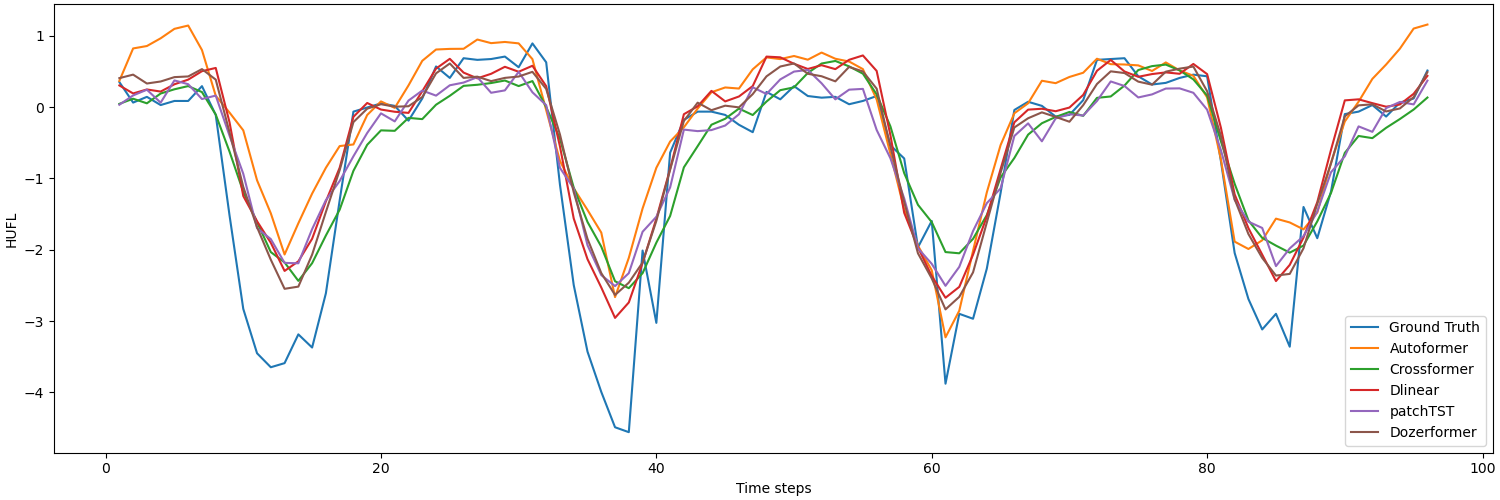
Figure 4: Visualizations of forecasting results on ETTh1 dataset at horizon 96.

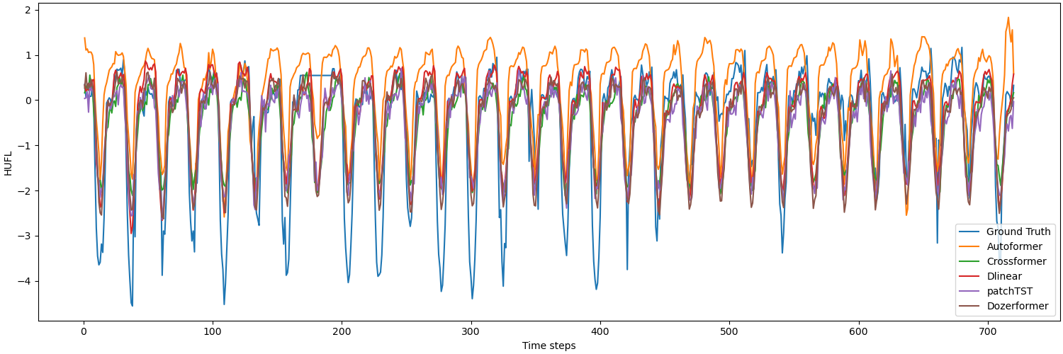
Figure 5: Visualizations of forecasting results on ETTh1 dataset at horizon 720.

A.3.4 More Ablation Studies

Figure 6 presents the results of an ablation study examining the impact of forecasting accuracy under different settings of local sizes, stride sizes, and vary starting sizes—key hyperparameters of the core Local, Stride, and Vary components of the Dozerformer. These hyperparameters influence the sparsity of the attention matrix, consequently affecting the efficiency of the Dozerformer in terms of computation and memory usage. A smaller local size, vary starting size, and a larger stride value result in a more sparse attention matrix, contributing to increased efficiency. It is noteworthy that an increase in historical time steps utilized in the attention mechanism does not necessarily lead to enhanced accuracy. The optimal local size varies based on the dataset’s characteristics, but we observe higher MSE values as the local size increases and more time steps are utilized. Regarding the stride value, it reaches an optimum of 9 for the ETTh1 and ETTm1 datasets, while it is 1 for the Weather datasets. For the vary value, a small value of 1 produces good performance in terms of accuracy and efficiency. In summary, we conclude that the selection of these hyperparameters varies across datasets. However, a sparse matrix, in general, performs better than a more dense attention matrix.

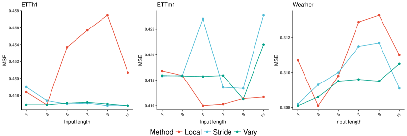
Figure 6: The forecasting results in terms of MSE for different Local, Stride, and Vary values at the horizon of 720.

The historical time step size is a crucial parameter for time series forecasting tasks, as it determines the model’s receptive field. In theory, a longer sequence length should enhance forecasting accuracy by providing the model with more historical information. However, most methods encounter challenges in aligning with this assumption. Figure 7 illustrates how different methods are influenced by the input sequence length. Remarkably, the Dozerformer consistently outperforms other methods for various sequence lengths in the ETTh1, ETTm1, and Weather datasets. The Exchange-Rate dataset is an exception; due to its lack of seasonality, all methods experienced a decline in accuracy with longer input sequences. Notably, an increase in input sequence length does not necessarily lead to improved accuracy for the Dozerformer. In contrast, for the remaining baseline methods, their performance tends to deteriorate as the input sequence length increases. We attribute this trend to longer input sequences incorporating more historical time steps that lack correlation with the forecasting target, thereby degrading the performance of these methods. The Dozerformer, by nature of its sparsity, is less affected, as it naturally excludes uncorrelated time steps from its attention mechanism.

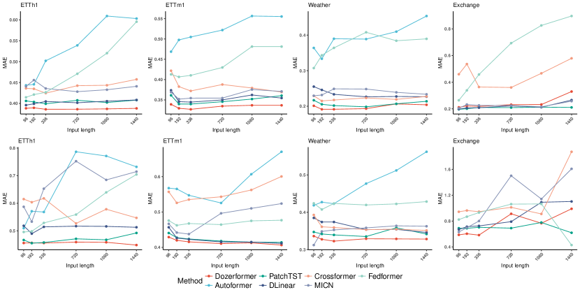
Figure 7: The forecasting results in terms of MAE for different look-back window sizes at horizons 96 and 720.

References

- Beltagy et al. (2020) Iz Beltagy, Matthew E. Peters, and Arman Cohan. Longformer: The long-document transformer. arXiv:2004.05150, 2020.
- Dosovitskiy et al. (2021) Alexey Dosovitskiy, Lucas Beyer, Alexander Kolesnikov, Dirk Weissenborn, Xiaohua Zhai, Thomas Unterthiner, Mostafa Dehghani, Matthias Minderer, Georg Heigold, Sylvain Gelly, Jakob Uszkoreit, and Neil Houlsby. An image is worth 16x16 words: Transformers for image recognition at scale. ICLR, 2021.
- Khan et al. (2022) Salman Khan, Muzammal Naseer, Munawar Hayat, Syed Waqas Zamir, Fahad Shahbaz Khan, and Mubarak Shah. Transformers in vision: A survey. ACM computing surveys (CSUR), 54(10s):1–41, 2022.
- Lai et al. (2018) Guokun Lai, Wei-Cheng Chang, Yiming Yang, and Hanxiao Liu. Modeling long-and short-term temporal patterns with deep neural networks. In The 41st international ACM SIGIR conference on research & development in information retrieval, pp. 95–104, 2018.
- Liu et al. (2022) Shizhan Liu, Hang Yu, Cong Liao, Jianguo Li, Weiyao Lin, Alex X Liu, and Schahram Dustdar. Pyraformer: Low-complexity pyramidal attention for long-range time series modeling and forecasting. In International Conference on Learning Representations, 2022.
- Nie et al. (2023) Yuqi Nie, Nam H. Nguyen, Phanwadee Sinthong, and Jayant Kalagnanam. A time series is worth 64 words: Long-term forecasting with transformers. In International Conference on Learning Representations, 2023.
- Petropoulos et al. (2022) Fotios Petropoulos, Daniele Apiletti, Vassilios Assimakopoulos, Mohamed Zied Babai, Devon K. Barrow, Souhaib Ben Taieb, Christoph Bergmeir, Ricardo J. Bessa, Jakub Bijak, John E. Boylan, Jethro Browell, Claudio Carnevale, Jennifer L. Castle, Pasquale Cirillo, Michael P. Clements, Clara Cordeiro, Fernando Luiz Cyrino Oliveira, Shari De Baets, Alexander Dokumentov, Joanne Ellison, Piotr Fiszeder, Philip Hans Franses, David T. Frazier, Michael Gilliland, M. Sinan Gönül, Paul Goodwin, Luigi Grossi, Yael Grushka-Cockayne, Mariangela Guidolin, Massimo Guidolin, Ulrich Gunter, Xiaojia Guo, Renato Guseo, Nigel Harvey, David F. Hendry, Ross Hollyman, Tim Januschowski, Jooyoung Jeon, Victor Richmond R. Jose, Yanfei Kang, Anne B. Koehler, Stephan Kolassa, Nikolaos Kourentzes, Sonia Leva, Feng Li, Konstantia Litsiou, Spyros Makridakis, Gael M. Martin, Andrew B. Martinez, Sheik Meeran, Theodore Modis, Konstantinos Nikolopoulos, Dilek Önkal, Alessia Paccagnini, Anastasios Panagiotelis, Ioannis Panapakidis, Jose M. Pavía, Manuela Pedio, Diego J. Pedregal, Pierre Pinson, Patrícia Ramos, David E. Rapach, J. James Reade, Bahman Rostami-Tabar, Michał Rubaszek, Georgios Sermpinis, Han Lin Shang, Evangelos Spiliotis, Aris A. Syntetos, Priyanga Dilini Talagala, Thiyanga S. Talagala, Len Tashman, Dimitrios Thomakos, Thordis Thorarinsdottir, Ezio Todini, Juan Ramón Trapero Arenas, Xiaoqian Wang, Robert L. Winkler, Alisa Yusupova, and Florian Ziel. Forecasting: theory and practice. International Journal of Forecasting, 38(3):705–871, 2022. ISSN 0169-2070. doi: https://doi.org/10.1016/j.ijforecast.2021.11.001. URL https://www.sciencedirect.com/science/article/pii/S0169207021001758.
- Shih et al. (2019) Shun-Yao Shih, Fan-Keng Sun, and Hung-yi Lee. Temporal pattern attention for multivariate time series forecasting. Machine Learning, 108:1421–1441, 2019.
- Vaswani et al. (2017) Ashish Vaswani, Noam Shazeer, Niki Parmar, Jakob Uszkoreit, Llion Jones, Aidan N Gomez, Ł ukasz Kaiser, and Illia Polosukhin. Attention is all you need. In I. Guyon, U. Von Luxburg, S. Bengio, H. Wallach, R. Fergus, S. Vishwanathan, and R. Garnett (eds.), Advances in Neural Information Processing Systems, volume 30. Curran Associates, Inc., 2017. URL https://proceedings.neurips.cc/paper_files/paper/2017/file/3f5ee243547dee91fbd053c1c4a845aa-Paper.pdf.
- Wang et al. (2023) Huiqiang Wang, Jian Peng, Feihu Huang, Jince Wang, Junhui Chen, and Yifei Xiao. Micn: Multi-scale local and global context modeling for long-term series forecasting. In International Conference on Learning Representations, 2023. https://openreview.net/forum?id=zt53IDUR1U.
- Wen et al. (2023) Qingsong Wen, Tian Zhou, Chaoli Zhang, Weiqi Chen, Ziqing Ma, Junchi Yan, and Liang Sun. Transformers in time series: A survey. In International Joint Conference on Artificial Intelligence(IJCAI), 2023.
- Wu et al. (2021) Haixu Wu, Jiehui Xu, Jianmin Wang, and Mingsheng Long. Autoformer: Decomposition transformers with Auto-Correlation for long-term series forecasting. In Advances in Neural Information Processing Systems, 2021.
- Wu et al. (2019) Zonghan Wu, Shirui Pan, Guodong Long, Jing Jiang, and Chengqi Zhang. Graph wavenet for deep spatial-temporal graph modeling. arXiv preprint arXiv:1906.00121, 2019. arXiv:1906.00121 https://doi.org/10.48550/arXiv.1906.00121.
- Wu et al. (2020) Zonghan Wu, Shirui Pan, Guodong Long, Jing Jiang, Xiaojun Chang, and Chengqi Zhang. Connecting the dots: Multivariate time series forecasting with graph neural networks. In Proceedings of the 26th ACM SIGKDD International Conference on Knowledge Discovery & Data Mining, 2020.
- Zaheer et al. (2020) Manzil Zaheer, Guru Guruganesh, Kumar Avinava Dubey, Joshua Ainslie, Chris Alberti, Santiago Ontanon, Philip Pham, Anirudh Ravula, Qifan Wang, Li Yang, et al. Big bird: Transformers for longer sequences. Advances in Neural Information Processing Systems, 33, 2020.
- Zeng et al. (2023) Ailing Zeng, Muxi Chen, Lei Zhang, and Qiang Xu. Are Transformers Effective for Time Series Forecasting?, pp. 11121–11128. AAAI Press, 2023. ISBN 978-1-57735-880-0. URL https://doi.org/10.1609/aaai.v37i9.26317.
- Zhang et al. (2023) Yifan Zhang, Rui Wu, Sergiu M. Dascalu, and Frederick C. Harris Jr au2. Multi-scale transformer pyramid networks for multivariate time series forecasting, 2023.
- Zhang & Yan (2023) Yunhao Zhang and Junchi Yan. Crossformer: Transformer utilizing cross-dimension dependency for multivariate time series forecasting. In International Conference on Learning Representations, 2023.
- Zhou et al. (2021) Haoyi Zhou, Shanghang Zhang, Jieqi Peng, Shuai Zhang, Jianxin Li, Hui Xiong, and Wancai Zhang. Informer: Beyond efficient transformer for long sequence time-series forecasting. In The Thirty-Fifth AAAI Conference on Artificial Intelligence, AAAI 2021, Virtual Conference, pp. 11106–11115. AAAI Press, 2021.
- Zhou et al. (2022) Tian Zhou, Ziqing Ma, Qingsong Wen, Xue Wang, Liang Sun, and Rong Jin. FEDformer: Frequency enhanced decomposed transformer for long-term series forecasting. In Proc. 39th International Conference on Machine Learning (ICML 2022), 2022.