Probing Disk Ice Content and PAH Emission Through Multiband MagAO+Clio Images of HD 141569

Abstract

We present resolved images of the inner disk component around HD 141569A using the Magellan adaptive optics system with the Clio2 1 - $5\mu$m camera, offering a glimpse of a complex system thought to be in a short evolutionary phase between protoplanetary and debris disk stages. We use a reference star along with the KLIP algorithm for PSF subtraction to detect the disk inward to about $0\hbox{$.\!\!^{\prime\prime}$}24\ (\sim 25$ au assuming a distance of 111 pc) at high signal-to-noise ratios at $L^{\prime}\ (3.8\mu$m), $Ls\ (3.3\mu$m), and narrowband $Ice\ (3.1\mu$m). We identify an arc or spiral arm structure at the southeast extremity, consistent with previous studies. We implement forward modeling with a simple disk model within the framework of an MCMC sampler to better constrain the geometrical attributes and photometry using our KLIP-reduced disk images. We then leverage these modeling results to facilitate a comparison of the measured brightness in each passband to find a reduction in scattered light from the disk in the $Ice$ filter, implying significant absorption due to water ice in the dust. Additionally, our best-fit disk models exhibit peak brightness in the southwestern, back-scattering region of the disk, which we suggest to be possible evidence of 3.3 $\mu$m PAH emission. However, we point out the need for additional observations with bluer filters and more complex modeling to confirm these hypotheses.

1 Introduction

Circumstellar disks offer unique opportunities to study how planets form and interact with their environments. Observations of disks reveal a broad range of developmental periods, ranging from young, gas-rich protoplanetary disks (e.g., HL Tauri; ALMA Partnership et al. 2015) to gas-depleted systems showcasing complex debris rings akin to the Asteroid Main Belt (e.g., Formalhaut; Gáspár et al. 2023). It is the transitional and “hybrid disk” stages that are of particular value as a laboratory in which to study the last stages of gas-giant and collisional stages of terrestrial planet formation. Young to intermediate-age disks ($\lesssim 10$ Myr) such as the HD 141569 system can thus help refine these theories with direct imaging of nascent planets or by observing characteristic features of early-stage planet formation such as spiral arms, gaps, and asymmetrical dust distribution (Wyatt, 2005).

The distribution of bulk compositions including water, carbon, and silicon in circumstellar disks may offer clues to the ultimate composition and evolution of planets (Shahar et al., 2019). One way to ascertain the presence of water ice in disks is to observe the scattered light at 3–4 $\mu$m including the water-ice absorption feature at $3.1\mu$m (Inoue et al., 2008). This method has revealed water ice in the scattering surface layers of the disks around HD 142527 (Honda et al., 2009), HD 100546 (Honda et al., 2016), and AB Aurigae (Betti et al., 2022).

Polycyclic aromatic hydrocarbons (PAHs) are an easily detected form of carbon in the disks around luminous stars. In response to ultraviolet (UV) excitation, these large molecules display distinct emission features in the 3-$20\mu$m spectral range; see the review by Tielens (2008) for a thorough discussion. Young disks are likely to be permeated with PAHs, but the uppermost disk layers receive the highest levels of UV flux and therefore have the highest PAH excitation rates (Siebenmorgen & Heymann, 2012). Because of this, it has been proposed (Seok & Li, 2017) that PAH emission can be a tracer for the gas-dominated disk atmosphere. Furthermore, given their stochastic heating mechanism (Draine & Li, 2001), PAH emission may be easily detected at large radial distances from the star on both the front and back sides, as long as we have a direct line-of-sight to the emitters. PAHs substantially impact circumstellar disk chemistry in the later evolutionary stages, acting as the formation site of, e.g., molecular hydrogen and water (Jonkheid et al., 2006).

HD 141569A is a young ($5\pm 3$ Myr; Weinberger et al. 1999) Herbig B9.5V/A0V star surrounded by a complex multi-ring system featuring gaps, spirals, arcs, and material asymmetries (see, e.g., Augereau et al. 1999; Weinberger et al. 1999; Mouillet et al. 2001; Clampin et al. 2003; Konishi et al. 2016; Mawet et al. 2017; Di Folco et al. 2020; Bruzzone et al. 2020; Singh et al. 2021). This unique disk is categorized as “hybrid” (Wyatt et al. 2015; Di Folco et al. 2020) in that it has substantial molecular gas (e.g., Zuckerman et al., 1995) and PAHs yet also displays the low optical depth of an early-stage debris disk. It may be in the final phases of dissipation and the last gasps of giant planet formation and migration. The host star is not variable (Alvarez & Schuster, 1981), is of intermediate mass with a luminosity of $27.5\pm 0.95L_{\odot}$ (calculated from the flux reported in Merín et al. 2004 and the distance of $111.6\pm 04$ pc reported in Gaia Data Release 3; Gaia Collaboration et al. 2023). Two M dwarf stars are located about 8 arcseconds from HD 141569A and may be bound companions (Weinberger et al., 2000), or have recently passed within 900 au (Reche et al., 2009). Gravitational effects either from these two low-mass companions (Augereau & Papaloizou, 2004; Reche et al., 2009) and/or from an unresolved giant planet (Wyatt, 2005) could be responsible for spiral arms seen in the disk.

The inner disk around HD 141569A ($R\leq 90$ au) has been the subject of multiple studies, but the results of many of these analyses raised further questions. Direct imaging at near-infrared wavelengths using VLT/SPHERE (Perrot et al. 2016; Singh et al. 2021) revealed a complex network of concentric rings from 40 to 90 au. Currie et al. (2016) reported additional independent detections of complex features in the $L^{\prime}$ band at $\sim 40$ au using Keck/NIRC2. However, it is important to note that these imaging efforts made use of angular differential imaging (ADI); thus these images are, due to the extended geometry and moderate inclination of the disk, inherently affected by observational bias (Milli et al., 2012). One way to mitigate this issue is using reference star differential imaging (RDI, Soummer et al. 2014; Ruane et al. 2019) to carry out the point-spread function (PSF) subtraction. Indeed, RDI with the Keck/NIRC2 vortex coronagraph mode by Mawet et al. (2017) revealed a more radially-extended $L^{\prime}$ profile from $\sim 20$ to 70 au that is distinctly different than the aforementioned ADI images in colocated regions. Mawet et al. (2017) also revealed the presence of a spiral or arc-like feature extended across the outer boundary of the southeast region of the disk, perhaps tying into more recent GPI $H$-band polarimetry direct imaging results by Bruzzone et al. (2020) who also identified a separate, but proximal spiral or arc candidate in the south disk ansa. A common conclusion in these studies (Perrot et al. 2016; Mawet et al. 2017; Bruzzone et al. 2020; Singh et al. 2021) is a significant brightness enhancement at the south ansa of the disk indicating a higher dust density distribution since the disk is optically-thin (Thi et al., 2014).

Gas is co-located with the dust disk. Thi et al. (2014) found $8.6\mu$m emission using VLT/VISIR which was thought to be from PAHs. Millimeter-wave range observations using ALMA/NOEMA unveiled significant asymmetry of ¹²CO $J=3\rightarrow 2$ emission in the western half of the SPHERE rings, possibly suggesting dynamical interactions between dust and gas in that region (Di Folco et al., 2020). Finally, recent observations using VLTI/GRAVITY revealed an additional ring of likely dusty material located at $\sim 1$ au (GRAVITY Collaboration et al., 2021).

In this work, we present imaging and forward modeling of the inner disk around HD 141569A, which imply the detection of water ice and reveal the spatial distribution of $3.3\mu$m PAH emission. We introduce the observations and detail the data reduction in the next section. In Section 3, we discuss our modeling procedures. We present the results of our forward modeling in Section 4 and discuss the most likely scenarios to explain our water ice and PAH emission hypotheses in Section 5. We use Section 6 to conclude and summarize our results as well as encourage avenues for future work.

2 Observations and Data Reduction

2.1 Observations

Table 1: HD 141569A and Reference Star Properties

	HD 141569A	HD 144271
R.A. (J2000)	15 49 57.75	16 05 8.49
Decl. (J2000)	-03 55 16.34	-3 31 39.40
Spectral Type	B9.5V/A0Ve	A0
$K$ (mag)	$6.82\pm 0.03$	$6.23\pm 0.02$
$L$ (mag)	$6.06\pm 0.07$	$6.21\pm 0.05$

Table 2: Clio Observation Log of HD 141569A and PSF Reference

Date	Time Start/End (UT)	Object	Band	Air Mass	$t_{\text{exp}}$ (s)	$N_{\text{coadds}}$	$N_{\text{exp}}$	$N_{\text{nods}}$	$\phi(^{\circ})$
2014 Apr 10	06:51/07:47	HD 141569A	$L^{\prime}$	1.1/1.1	1	20	121	3	-15/14
2014 Apr 10	07:54/09:15	HD 144271	$L^{\prime}$	1.1/1.1	0.75	20	80	2	9.5/41
2014 Apr 10	08:12/08:57	HD 141569A	$L^{\prime}$	1.1/1.2	0.75	20	118	3	25/40
2014 Apr 11	05:58/06:39	HD 141569A	$Ls$	1.1/1.1	2	10	90	2	-34/-19
2014 Apr 11	06:44/06:52	HD 144271	$Ls$	1.1/1.1	2	10	20	1	-22/-19
2014 Apr 11	06:56/07:19	HD 141569A	$Ls$	1.1/1.1	2	10	58	1.5	-10/2
2014 Apr 12	05:22/05:31	HD 141569A	$Ls$	1.2/1.2	2.5	10	60	3	-43/-41
2014 Apr 12	05:58/06:03	HD 144271	$Ls$	1.1/1.1	2.5	5	20	1	-37/-36
2014 Apr 12	06:06/06:16	HD 141569A	$Ls$	1.1/1.1	2.5	10	20	1	-30/-27
2014 Apr 12	07:22/07:31	HD 141569A	$Ls$	1.1/1.1	2.5	10	20	1	5/10
2014 Apr 12	08:17/08:21	HD 144271	$Ls$	1.1/1.1	2.5	4	20	1	24/25
2015 May 30	02:46/03:17	HD 141569A	$Ice$	1.2/1.1	14	3	43	2	-35/-23
2015 May 30	03:22/03:51	HD 144271	$Ice$	1.1/1.1	14	3	40	2	-27/-14
2015 May 30	03:55/04:52	HD 141569A	$Ice$	1.1/1.1	10	2	160	4	-5/23
2015 May 30	04:55/05:09	HD 144271	$Ice$	1.1/1.1	10	2	42	1	17/24

Notes. $t_{\text{exp}}$: single frame exposure time; $N_{\text{coadds}}$: number of coadded frames per image; $N_{\text{exp}}$: number of images; $N_{\text{nods}}$: number of ABBA nod sequences; $\phi$: start/end parallactic angle.

We obtained non-coronagraphic diffraction-limited images of HD 141569A (spectral type B9.5-A0, K=6.8 mag, L=6.1 mag) and PSF reference HD 144271 (spectral type A0, K=6.2 mag, L=6.2 mag) using the 6.5 m Magellan Clay telescope at Las Campanas Observatory (LCO) on the following nights: UT 2014 April 9 - 11, UT 2015 May 28 and 29, and UT 2018 April 28. for reference, we include useful properties of our targets in Table 1. For all observations, we used the Magellan Adaptive Optics system (MagAO; Morzinski et al. 2016) with the $1-5\mu$m Clio-2 instrument in imaging mode (Clio hereafter; Morzinski et al. 2015) configured with its narrow camera that provided a plate scale of $0\hbox{$.\!\!^{\prime\prime}$}01585$ per pixel and $16"\times 18"$ field of view. To facilitate RDI, we observed our target and reference stars with the rotator off to stabilize the pupil with respect to the detector focal plane. We performed ABBA nod sequences for our target and reference stars where the telescope was nodded by several arcseconds and dithered by a few tenths of an arcsecond for sky background and bad pixel removal during post-processing. To enable deeper disk images, we selected exposure times to saturate the detector out to about $0\hbox{$.\!\!^{\prime\prime}$}07$ from the star. At the end of each nod sequence, we collected photometric calibration exposures (i.e., unsaturated images). We logged observational circumstances for each dataset that produced a final reduced image of acceptable quality in Table 2 (some observations were carried out in poor weather, see below).

We observed the target and reference using the $L^{\prime}$ $(3.8\mu$m) filter on the nights of UT 2014 April 9, UT 2015 May 28, and UT 2018 April 28. Conditions on the first night were initially excellent with $0\hbox{$.\!\!^{\prime\prime}$}5$ seeing, but the seeing became variable during the latter half of this dataset prompting us to exclude the last 118 science frames (out of 240 total). Conditions on UT 2015 May 28 and UT 2018 April 28 were cloudy, with extinction affecting image quality and AO performance significantly so we ignored data from these nights in our analysis.

We collected images in the $3.3\mu$m filter ($Ls$ for “L-short”) on the nights of UT 2014 April 10 and 11. Technical issues with the AO system along with cloudy conditions resulted in images limited in both quality and quantity for the first night. Conditions for UT 2014 April 11 were much improved and photometric, with seeing ranging from $0\hbox{$.\!\!^{\prime\prime}$}5$ to $0\hbox{$.\!\!^{\prime\prime}$}75$.

We imaged through a narrowband $Ice$ $(3.1\mu$m) filter on the nights of UT 2014 April 11 and UT 2015 May 29. The seeing on the second night was quite good at $0\hbox{$.\!\!^{\prime\prime}$}6$ - $0\hbox{$.\!\!^{\prime\prime}$}7$ and very stable. The internal optics of Clio create an illumination artifact in the center of the detector (Morzinski et al., 2015). Both the target and reference stars were imaged close to the center of the detector by mistake. This unfortunately caused an optical ghost to propagate through to the final image which manifests as a circular oversubtracted region in the final reduced disk image just east of the star. The final reduced image using data from the first night was comparatively of lesser quality perhaps due to a moderate amount of sky rotation over the dataset ($\sim 39^{\circ}$). Because of the residual Airy pattern left in the final image, preliminary modeling using the data from UT 2014 April 11 produced models with non-physical parameters, so we refrained from using these data in our study.

Additionally, for the night of UT 2014 April 11, we obtained data at $2.15\mu$m ($Ks$ for “K-short”). Because of time lost to an AO problem, the amount of sky rotation was only $\sim 35^{\circ}$. We obtained only a small library of 16 reference PSF images for the RDI reduction (compared to 95 target images). Additionally, Clio’s performance at $Ks$ is limited due to detector read noise. We did not detect any disk components in these data.

As a result of these various issues, we only included the $L^{\prime}$ data taken on UT 2014 April 9, the $Ls$ data taken on UT 2014 April 12, and the $Ice$ data taken on UT 2015 May 29 in our modeling efforts (see Section 3). For each of these three passbands we treated the libraries of target and reference star images as separate datasets and applied all data reduction steps mentioned below consistently to each.

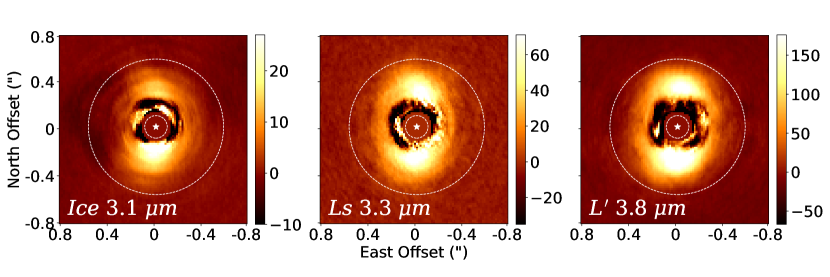
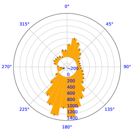
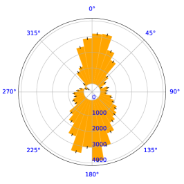
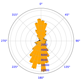
Figure 1: Top: Final KLIP-RDI reductions using MagAO+Clio data at $L$-band showing the inner disk component in a north-up, east-left orientation. The colorbar shows pixel values in counts/s. Bottom: Radar plots where the wedges portray the summed pixel counts in the above images in $10^{\circ}$ annular slices to quantify the azimuthal flux in our KLIP-RDI images. The $36$ annular slices are defined in the region between the two dotted white lines, about $0\hbox{$.\!\!^{\prime\prime}$}19$ to $0\hbox{$.\!\!^{\prime\prime}$}57$, with the black ticks at the end of each orange wedge representing the $3\sigma$ scatter on the pixel counts in each slice.

2.2 Data Reduction and PSF Subtraction

To prepare our data for background subtraction, we divided each image by the number of coadds followed by a linearity correction using the procedure outlined in Morzinski et al. (2015). We then divided each image by its exposure time to convert pixel values to counts/s. To remove the sky and telescope thermal background in our images, we assumed that the sky emission was stable enough to use as suitable background estimates for the images at the other nod position. For a given exposure, we created a background estimate using a median stack made from a sequence of counter-nod images that were captured closest in time. We employed a least-squares routine to determine the scale factor and offset that minimizes the residuals between this background estimate and a given target image ensuring that any stars or detector artifacts inconsistent between the two images were masked digitally. We extracted $128\times 128$ pixel $(2"\times 2")$ images centered on the star and then used a phase cross correlation routine to register, with sub-pixel accuracy, all thumbnail images to the first exposure of HD 141569A in the sequence (Guizar-Sicairos et al., 2008).

Since MagAO provides exceptional PSF stability and delivers high Strehl ratios in the 1-5$\mu$m regime (Morzinski et al., 2015), we performed PSF subtraction using RDI coupled with the Karhunen-Lo$\grave{\text{e}}$ve Image Projection (KLIP; Soummer et al. 2012) algorithm, which is an application of Principal Component Analysis that assumes discrete-to-discrete operations with Gaussian statistics. We made use of the Python-based pyKLIP package (Wang et al., 2015) to perform KLIP-RDI on our data with images of HD 144271 (see Section 2.1) serving as our reference PSF library.

The top row in Figure 1 shows the final KLIP-reduced images for each passband. The bottom row shows radar plots illustrating the summed pixel values in annular slices between $0\hbox{$.\!\!^{\prime\prime}$}19$ and $0\hbox{$.\!\!^{\prime\prime}$}57$ as marked by the two white dotted lines in the images. These radar plots represent the azimuthal flux distribution detected in the inner disk region.

One of the challenges when using KLIP-RDI to remove starlight to reveal faint underlying circumstellar objects is choosing the optimal number of KLIP modes to use when forming the basis such that self- or over-subtraction is minimal (Milli et al., 2012). Given that this inner disk component has been directly imaged previously (Currie et al. 2016; Perrot et al. 2016; Mawet et al. 2017; Bruzzone et al. 2020; Singh et al. 2021) we optimized the $S/N$ of the brightest part of the previously known disk ansae by performing a grid search over the number of KLIP modes and the size of the central software star mask (i.e., the IWA). We fixed the outer working angle (OWA) of the annular search region to OWA $=80\text{ pixels}\approx 1\hbox{$.\!\!^{\prime\prime}$}3$.

To estimate the noise maps that we used in calculating $S/N$ as well as in our forward model fitting, we followed Lawson et al. (2020) and computed the noise at every radial location using concentric measurement annuli of 1 FWHM width to compute the standard deviation in each of our KLIP-RDI images. To improve our estimation, we made use of software masks to exclude the prominent north and south disk ansae in our noise calculation. We note that it is difficult to compute the underlying noise because there are few to no pixels at each radius that do not have disk flux.

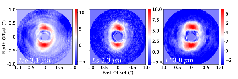
Figure 2: S/N per pixel maps of KLIP-RDI reduced images of the $L^{\prime}$, $Ls$, and $Ice$ datasets where the central star region has been overlaid with a software mask of radius $r=0\hbox{$.\!\!^{\prime\prime}$}13$.

The best S/N was achieved using an IWA of 8 pixels ($0\hbox{$.\!\!^{\prime\prime}$}13$) coupled with a basis consisting of 3, 6, and 7 modes for $Ice$, $Ls$, and $L^{\prime}$ datasets respectively. Figure 2 shows the corresponding S/N results for our final reduced images. The full scope of this grid search is summarized in Table 3. We note that for our $Ls$ datasets imaged on UT 2014 April 10 and 11 (start of night), we additionally optimized the KLIP reduction such that $S/N$ of a spiral/arc feature is maximized; these results are shown in Figure 3. Measuring the $S/N$ of the spiral/arc feature in the right panel image in Figure 3 from the white arrow down to the southern disk region yields around 1.5 to 2. We repeated the KLIP data reduction for this higher quality $Ls$ dataset from UT April 11 but instead used angular differential imaging to better preserve the footprint of a potential point source (marked in the right panel of Figure 3 with a white arrow). This analysis yielded a $S/N$ of 2.7 for the candidate point source using $27/60$ KLIP modes for the PSF subtraction.

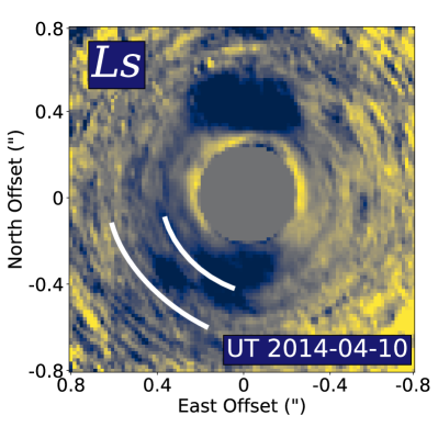
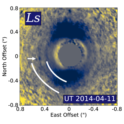
Figure 3: Inverted color map images of our observations at $Ls$ corresponding to the nights of UT 2014-04-10 to 11. The pixel values have been multiplied by $r^{2}$ to bring out faint structures in the outer regions of the disk. White curves bound the arc or spiral-like structure to the southeast in each image, which was previously identified in Mawet et al. (2017). The right image, which corresponds to the higher quality dataset, hints at a point source-like feature at the terminus of the arc or spiral arm.

Table 3: Chosen KLIP Parameters Based on $S/N$ Optimization

	Date Obs. (UT)	$N_{\text{modes}}$	IWA $(")$	OWA $(")$
$L^{\prime}$	2014 Apr 09	7/80	0.13	1.3
$Ls$	2014 Apr 11	6/40	0.13	1.3
${}^{\dagger}Ls$	2014 Apr 10	8/20	0.22	1.3
${}^{\dagger}Ls$	2014 Apr 11	9/40	0.19	1.3
$Ice$	2015 May 29	3/81	0.13	1.3

Notes. $N_{\text{modes}}$: number of KLIP modes; IWA: inner working angle; OWA: outer working angle.
^† KLIP parameters used to optimize the $S/N$ of spiral arm feature for Figure 3.

3 Disk Modeling

3.1 Model Description

We performed forward modeling to further characterize the geometry of the inner disk using our total intensity images taken on the nights of UT 2014-04-09 $(L^{\prime})$, UT 2014-04-11 $(Ls)$, and UT 2015-05-29 $(Ice)$ (see Section 2.1).

Following Chen et al. (2020), we explored the geometrical parameters and grain sizes in the 20 to 70 au region of the inner disk by implementing the DiskFM pipeline (Mazoyer et al., 2020) of the pyKLIP package which accomplishes forward modeling based on the principles presented in Pueyo (2016). Additionally, we used the Markov-Chain Monte Carlo (MCMC) sampler package, emcee (Foreman-Mackey et al., 2013), as a wrapper to DiskFM for estimating the parameter values.

We generated scattered light disk models at $3.8\mu$m, $3.3\mu$m, and $3.1\mu$m to use in our forward modeling and assumed that the inner disk is optically thin (Bruzzone et al. 2020; Thi et al. 2014) to interpret model fits to the observed brightness asymmetry. Our final models were limited to a single ring geometry since preliminary trials with multi-ring models (inspired by the ringlets presented in Perrot et al. 2016) produced poor fits to our data. We made use of the disk model in stellocentric coordinates from Ren et al. (2019), which is a modified form of that in Millar-Blanchaer et al. (2015):

$$\rho(r)\propto\left[\left(\frac{r}{r_{c}}\right)^{-2\alpha_{\text{in}}}+\left(\frac{r}{r_{c}}\right)^{-2\alpha_{\text{out}}}\right]^{-\frac{1}{2}},$$ (1)

where $r$ is the radial coordinate, $r_{c}$ is the critical radius of the disk corresponding to the location of the peak dust density, and $\alpha_{\text{in}}$ and $\alpha_{\text{out}}$ denote the radial power laws of the surface brightness interior and exterior to the critical radius, respectively. Note that we constrained $\alpha_{\text{in}}$ to be positive and $\alpha_{\text{out}}$ to be negative for our modeling. We modeled the vertical distribution $Z(r,z)$ (normal to the disk midplane) using a Gaussian profile, i.e.,

$$Z(r,z)\propto\exp{\left[-\left(\frac{z}{h_{0}r^{\beta}}\right)^{2}\right]},$$ (2)

where $z$ is the vertical axis coordinate, $h_{0}$ is the constant aspect ratio, and $\beta$ is the dust flaring component. We arbitrarily fixed the disk aspect ratio to $h_{0}=0.02$ and the dust flaring exponent was set to $\beta=1$ (non-flaring), supported by our above-mentioned assumption that the dust is optically thin. As also found by Mawet et al. (2017), our data allow limited constraint on the dust density radial power law indices $\alpha_{\text{in}}$ and $\alpha_{\text{out}}$, so we adopted $\alpha_{in}=1.5$ and $\alpha_{out}=-9$ by visual inspection of the forward models.

Table 4: DiskFM Modeling Results for HD 141569A

Parameter${}^{\text{a}}$		Range Explored${}^{\text{b}}$		Best Fit Values${}^{\text{c}}$			Mawet et al. (2017)
				$Ice$	$Ls$	$L^{\prime}$
$\log_{10}R_{c}$ (au)		(25, 50)		$40.39\pm 0.50$	$39.62\pm 0.43$	$39.07\pm 0.53$	$39\pm 4$
$i(^{\circ})$		(30, 80)		$47.47\pm 1.32$	$47.61\begin{subarray}{c}+0.98\\ -1.04\end{subarray}$	$48.10\begin{subarray}{c}+0.97\\ -1.07\end{subarray}$	$53\pm 6$
$PA(^{\circ})$		(-20, 20)		$-2.45\begin{subarray}{c}+0.90\\ -0.93\end{subarray}$	$-2.19\pm 0.90$	$-0.68\begin{subarray}{c}+0.92\\ -0.94\end{subarray}$	$-11\pm 8$
$dx$ (au)		(-15, 15)		$-0.58\pm 0.57$	$-5.99\begin{subarray}{c}+0.78\\ -0.74\end{subarray}$	$-3.14\begin{subarray}{c}+1.30\\ -1.50\end{subarray}$	$-2\pm 7$
$dy$ (au)		(-10, 10)		$1.23\begin{subarray}{c}+0.55\\ -0.53\end{subarray}$	$1.96\pm 0.41$	$2.34\begin{subarray}{c}+0.46\\ -0.48\end{subarray}$	$0\pm 4$
$\log_{10}a_{\text{min}}$ ($\mu$m)		(0.001, 10)		$0.62\begin{subarray}{c}+0.02\\ -0.01\end{subarray}$	$0.66\begin{subarray}{c}+0.02\\ -0.01\end{subarray}$	$0.79\begin{subarray}{c}+0.03\\ -0.04\end{subarray}$	$0.1$
$F$ (mJy)${}^{\text{d}}$				$19.48\pm 0.22$	$26.34\pm 0.23$	$31.31\pm 0.27$

Notes.
${}^{\text{a}}$ We included parameter $N$ in our modeling to handle the flux normalization, but it is not shown in this table.
${}^{\text{b}}$ We assumed uniform prior distributions for all parameters except the disk midplane offset $dx$ which required Gaussian prior regularization due to parameter space degeneracies.
${}^{\text{c}}$ 16th, 50th, and 84th percentiles.
${}^{\text{d}}$ We include the total flux of the modeled disk in mJy units which we computed by summing the best-fit model; see text.

We generated the intensity of the model by computing a brightness integral for each pixel $(x^{\prime},y^{\prime})$ along the line of sight $(z^{\prime})$ (where primed coordinates denote the detector frame) expressed as

$$I(x^{\prime},y^{\prime})=I_{0}+\int_{z^{\prime}=-R_{2}}^{R_{2}}dz^{\prime}\frac{N_{0}}{r^{2}}\rho(r)Z(r,z)P(\theta),$$ (3)

where $P(\theta)$ is the scattering phase function (SPF) and $R_{2}$ marks the user-set outer boundary where the dust density defaults to zero (i.e., the observed outer radius of the disk). To speed calculations, we defined $R_{2}$ to correlate tightly to the edge of the observed disk signal in our KLIP-RDI images since we assume the radial extent of the disk along the major axis is the largest spatial dimension. This resulted in an elliptical modeling region with a major axis of $0\hbox{$.\!\!^{\prime\prime}$}54$ and minor axis of $0\hbox{$.\!\!^{\prime\prime}$}34$ and rotated such that the major axis aligns with north-south; $R_{2}$ corresponds to the outer boundary for the minimization region as shown as the dashed white ellipse in the KLIP-RDI images in Figure 5. Additionally, $I_{0}$ and $N_{0}$ are parameters representing a constant offset and scale factor to handle flux normalization respectively. The disk coordinate system undergoes tilting with respect to the observer by varying an inclination parameter $i$ and the position angle $PA$ manages the clocking with respect to the sky. The scattering angle $\theta(x^{\prime},y^{\prime},z^{\prime})$ is a function of position in the image.

We used a custom SPF, which is calculated from simulated agglomerated debris particles (ADPs) (see Zubko et al. 2015; Arnold et al. 2022 for a full description). The irregular, porous shapes of these ADPs (porosity of 70-80%) attain a more realistic representation of the shapes of dust grains than a distribution of, e.g., solid or hollow spheres. We created a dust grain size distribution $n_{a}$ based on a minimum grain size $a_{\text{min}}$, a maximum grain size $a_{\text{max}}$, and a power law index $q$ such that $dN/da\propto a^{-q}$. We then obtain a complex index of refraction, typical of astronomical silicates, using results from Draine (2003a) and Draine (2003b) by linearly interpolating at our wavelength of interest. Since the lookup tables from Arnold et al. (2022) parameterize the scattering efficiencies by complex index of refraction and size parameter, we use the results from the above steps to query the scattering efficiencies for angles $\theta=[0,\pi]$ to obtain the custom SPF. For our modeling, we fixed the maximum grain size to $a_{\text{max}}=1$ cm and the size distribution exponent to $q=3.5$, but assigned the minimum grain size $a_{\text{min}}$ as a free parameter.

In total, we fit for 7 parameters in our forward modeling efforts: the critical radius $R_{c}$, the inclination $i$, the position angle $PA$, the stellar offsets in the disk’s midplane $xy$-directions $dx$ and $dy$, the flux normalization $N$, and the minimum grain size $a_{\text{min}}$.

Importantly, we note that we chose a simple scattered-light disk model appropriate for measuring the KLIP-RDI throughput and observed disk surface brightness. We expect that our model may not match more detailed physical attributes of the disk.

3.2 MCMC Parameter Estimation

To find the key geometric properties that best fit our reduced disk images, we used the Markov-Chain Monte Carlo (MCMC) sampler emcee package (Foreman-Mackey et al., 2013). The range of values probed for all fitted parameters are shown in Table 4 with the exception of the model flux scaling parameter $N$. In short, our simple disk models are forward modeled using DiskFM (Mazoyer et al., 2020) to estimate the algorithmic artifacts and throughput loss using KLIP. An overview of the full forward modeling procedure is as follows:

1. Generate a disk model using the method outlined in 3.1.

2. Convolve the disk model with the empirically-measured, unsaturated instrument PSF (see Sec. 2.1) to simulate a model image.

3. Use the pyKLIP DiskFM pipeline to produce a forward model (FM) using the same KLIP parameters as the final KLIP-RDI image.

4. Gauge the goodness of fit of these results using the standard $\chi^{2}$ metric:

   $$\chi^{2}=\sum_{S}\frac{(\text{Data}-\text{FM})^{2}}{\text{Uncertainty}^{2}},$$ (4)

where $S$ is the zone of interest where $e^{-\chi^{2}/2}$ is maximized; see Section 4.2. Our estimate for the uncertainty is described in Section 2.2.

To assure convergence, we repeated the enumerated steps above until the number of iterations exceeded 50 times the autocorrelation time of the chains. This amounted to modeling 564.0k, 808.4k, and 611.0k disk models for $L^{\prime}$, $Ls$, and $Ice$ bands respectively. We assumed uniform prior probability distributions for all fitted parameters except $dx$, which we regularized with a Gaussian prior ($\sigma=2$ au) centered on zero. Without regularization, degeneracies in the parameter space resulted in disk models we regarded as non-physical. Additionally, in a burn-in phase, we ignore the number of initial steps in each chain equal to twice the autocorrelation time, as recommended in the documentation for emcee.

3.3 Photometric Calibration

We use our short, unsaturated images of HD 141569 for photometric calibration. We performed sky background subtraction on these images using the same procedures as in Section 2.2, divided by the exposure time, and then summed the counts in an aperture of radius $r=3\hbox{$.\!\!^{\prime\prime}$}2(\approx 30\lambda/D$). We inspected curves of growth (i.e., summed counts as a function of aperture radius) for each background-subtracted calibration frame and excluded results from frames where the curve did not asymptote, which indicated that the background subtraction was sub-optimal. We then averaged our aperture photometry for non-rejected calibration frames.

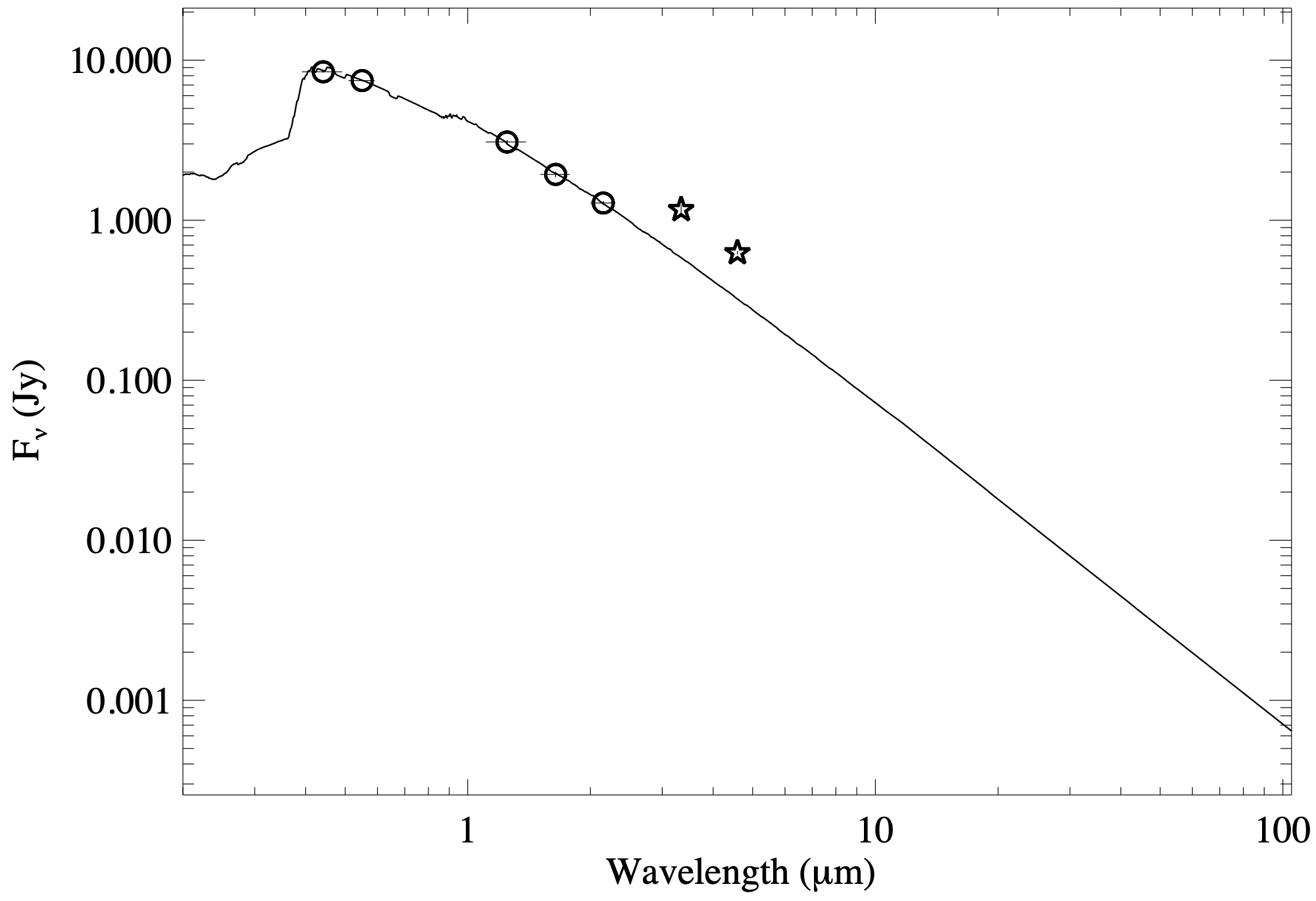
Figure 4: Kurucz model fit ($T_{\text{eff}}=10000$ K, $\log g=4.5$); with a reddening extinction correction of $A_{V}=0.35$ mag) to HD 141569A BVJHK catalog magnitudes which are represented by the circles. We plot AllWISE (Cutri et al., 2014) W1 and W2 photometry as stars to show a poor fit to our model compared to the visible and near-infrared data. We ignore the AllWISE photometry when calculating our photometric calibration.

Table 5: Comparison of photometric calibration factors calculated using images of HD 141569 A and PSF reference HD 144271 to convert pixel values from counts/s to Jy/arcsec².

	$Ice$	$Ls$	$L^{\prime}$
HD 141569 A	2.57e-11	7.19e-12	2.43e-12
HD 144271	2.59e-11	7.33e-12	2.54e-12

To convert our final reduced images and disk models from counts/s to mJy/arcsec², we use the ratio of the model flux density (in Jy units) to the average counts/s measured in our unsaturated calibration exposures of HD 141569A. To calculate HD 141569A’s flux density in each of our filters, we model its photosphere with a Kurucz model ($T_{\text{eff}},\log g=4.5$) and fitted it to catalog $BV$ (Tycho-2; Høg et al. 2000) and $JHK$ (2MASS; Skrutskie et al. 2006) magnitudes of HD 141569A with a reddening extinction correction of $A_{V}=0.35$ mag. We note that we ignore WISE W1 and W2 photometry because they constitute a poor fit to our model possibly due to contamination from the two M-dwarf companions as shown in Figure 4. As a sanity check and to ensure that excess infrared flux from the disk was not significantly contaminating our photometry, we repeated the above methods for calibration frames of the reference star HD 144271 and obtained calibration factors to within about 1%, 2%, and 4% for $Ice$, $Ls$, and $L^{\prime}$ filters respectively. All calibration factors are shown in Table 5 for comparison.

4 Results

Figure 5: Forward modeling results for $L^{\prime}$, $Ls$, and $Ice$ images where the color bar for the three leftmost columns are in surface brightness units of mJy/(”)². The red circle in the best model images in the first (leftmost) column indicate the location of the star. We mark the zone where $\chi^{2}$ is evaluated between the dashed white lines in the KLIP-RDI images shown in the third column. The we used the best-fit models in the leftmost column to compute the flux density of the disk by multiplying the models by the squared pixel scale and summing the resulting pixel values; we appended the resulting values to Table 4. The best-fit models for the $Ice$ and $L^{\prime}$ bands assume nearly isotropic scattering while the model for the $Ls$ passband is highly asymmetric due to a stellar offset in the x-direction. The front side of the disk is the eastern (left) half.

4.1 Potential Spiral Arm and Point-like Feature

Notable features in our $Ls$ KLIP-RDI images include an arc or spiral-like feature to the southeast, similar to what was seen by Mawet et al. (2017) and Currie et al. (2016) at $L^{\prime}$, by Perrot et al. (2016) at shorter wavelengths in the near-infrared, and by Konishi et al. (2016) in the visible. Figure 3 shows our $Ls$ KLIP-RDI images that were reduced with specific KLIP parameters to bring out faint spiral or arc feature (see Section 2.2) and where each pixel was multiplied by $r^{2}$ to better show the dust density distribution and faint outer features. The arc or spiral feature is traced by red arrows. The image from observations on UT 2014-04-11 clearly show an arc or spiral feature originating in the southern-most region of the inner disk and trailing up to the northeast, terminating at $\sim 0\hbox{$.\!\!^{\prime\prime}$}5$ to the east of the star. Interestingly, there appears to be a point-like source at the end of the arc or spiral feature. Although the night of UT 2014-04-10 presented poor observing conditions resulting in a final KLIP-RDI image of poor quality, the arc or spiral-like feature is still discernible but the point-like source is not. These features are not recovered at any other passbands in our data.

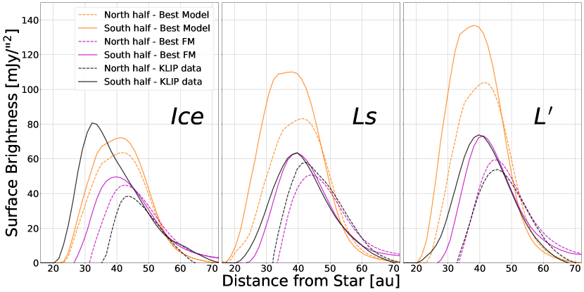
Figure 6: Surface brightness profiles extracted along the major axis using aperture photometry ($r_{\text{ap}}=\frac{\lambda}{2D}\approx 0\hbox{$.\!\!^{\prime\prime}$}06$) of the best-fit models for our HD 141569A disk images at $Ice$ (3.1 $\mu$m), $Ls$ (3.3 $\mu$m), and $L^{\prime}$ (3.8 $\mu$m). Dashed lines represent profiles across the north half of the disk while solid lines represent profiles for the south half. We denote profiles for the best-fitting disk model, best-fitting model convolved then forward modeled, and the final KLIP-RDI reduced image with orange, magenta, and black lines respectively. The best-fitting model profiles represent the disk photometry without the throughput loss due to the KLIP algorithm.

4.2 Modeling results

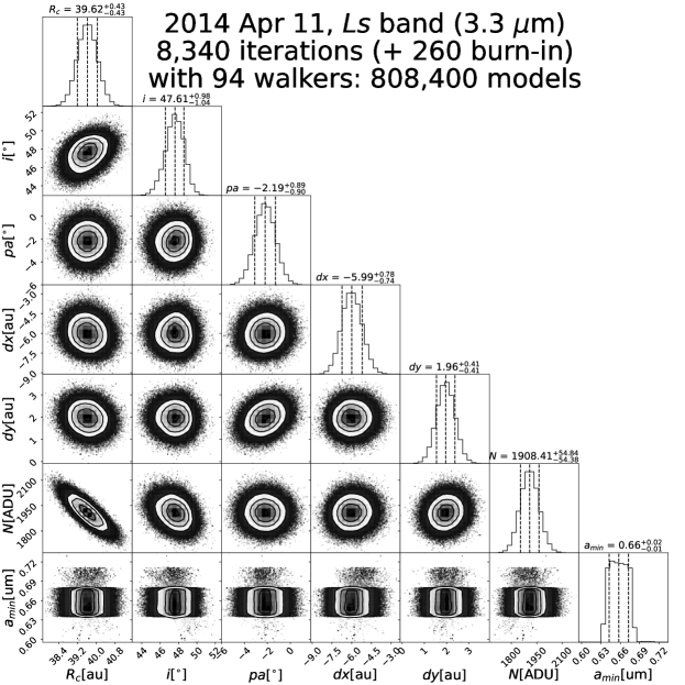
Figure A2: Same as Figure A1, but for the $Ls(3.3\mu m$) band data.

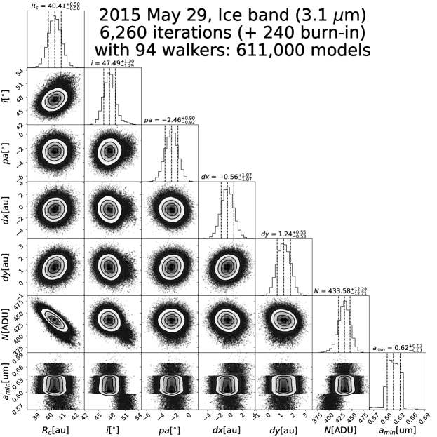
Figure A3: Same as Figure A1, but for the $Ice(3.1\mu m$) band data.

The final corner plots from our analysis as well as further information on the modeling parameters are shown in Figure A1, Figure A2, and Figure A3 in Appendix A. For each passband, Figure 5 shows our best-fit disk models, their forward models, the final KLIP-RDI images, and the S/N of the residuals in columns one through four respectively. We mark the location of the star with a red circle and bounded the zone where $\chi^{2}$ was minimized with white dashed lines. Note that some signal appears to be excluded interior to the inner boundary of this zone, but the extent to which the non-negative pixel values in these high speckle noise regions represent the inner disk is unclear.

4.2.1 Disk Geometry

The best-fit parameters from our forward modeling are summarized in Table 4 along with a comparison to $L^{\prime}$ results from Mawet et al. (2017). Best-fit values for the geometrical parameters are consistent within $3\sigma$ between the 3 passbands with the exception of the $dx$ stellar offset. We assume that the east side of the disk is closest to us from polarimetric imaging results (Bruzzone et al. 2020; Singh et al. 2021) and thus should exhibit strong forward scattering (assuming realistic dust grain properties) relative to the west side. However, our best fit models at $L^{\prime}$ and $Ls$ exhibit a lower flux on the eastern half. The model accomplishes this by inducing $dx$ and $dy$ stellar offsets (i.e., the disk is shifted along its midplane) thus placing the northeast part of the disk farther from the star. The $L^{\prime}$ and $Ls$ models hint at an offset of about 3 and 6 au in the negative $x$-direction in our stellocentric coordinates while the $Ice$ model prefers an offset of about 0.5 au in the negative $x$-direction, which is significantly different from the $Ls$ result. These offsets could manifest in the model fit due to other physical phenomena; see below (Section 5.1). However, this modest eastward offset for the $Ice$ model may be due to the circular oversubtraction artifact (see Figure 1). Despite these disagreements in best-fitting $dx$ values, they are all consistent with the $L^{\prime}s$ model from Mawet et al. (2017). We discuss implications of asymmetric dust density or gas in the disk from these stellar offsets below in Section 5.1.

S/N maps of the residuals between the best forward model and the KLIP-reduced data of the inner disk show an enhancement in the $Ice$ passband in the south ansa region of the disk that peaks at $\sim 3\sigma$; this same feature appears at $L^{\prime}$ in the residuals in Mawet et al. (2017). The residuals map at $Ls$ also displays a curiously small feature at $\sim 5\sigma$ significance to the north and immediately outside the central star mask. However, this may be a false positive given the small spatial extent of this feature and that it resides close to the high speckle noise region close in to the star. Similar features are seen in the $L^{\prime}$ residuals map at roughly the same radial distance, but at a lower significance.

4.2.2 Dust Grain Properties

For all our models, we fixed the maximum grain size to $a_{\text{max}}=1$ cm and the size distribution exponent to $q=3.5$. We obtained a best-fit minimum grain size $a_{\text{min}}$ of $0.62\begin{subarray}{c}+0.02\\ -0.01\end{subarray}\mu$m, $0.66\begin{subarray}{c}+0.02\\ -0.01\end{subarray}\mu$m, and $0.79\begin{subarray}{c}+0.03\\ -0.04\end{subarray}\mu$m for $Ice$, $Ls$, and $L^{\prime}$ bands respectively suggesting a majority of the scattering is due to sub-micron grains. Though the median values of these best-fit values differ between the 3 passbands, they are all consistent to within $3\sigma$. Further, this specific combination of grain parameters results in a disk model that scatters more or less isotropically which is perhaps unsurprising since our data probes a limited range of scattering angles (i.e., we only measure high S/N near the disk ansae). For completeness, we also performed forward modeling using a Henyey-Greenstein SPF which yielded a best-fitting disk model that isotropically scatters, but we omit those results from this paper in favor of results from the more realistic SPF calculated using the ADP scattering efficiencies from Arnold et al. (2022). Nonetheless, these results are consistent with the analysis shown in Currie et al. (2016) and Mawet et al. (2017) who also found isotropically-scattering disk models to best fit their total intensity images at $L^{\prime}$.

4.2.3 Disk Photometry

We extracted the disk surface brightness along the major axis in our best-fit models and KLIP-RDI reduced images using aperture photometry with aperture size set to $r=\lambda/(2D)\approx 0\hbox{$.\!\!^{\prime\prime}$}06$. The resulting profile curves are shown for the best-fit models (orange lines), forward models (magenta lines), and the reduced images (black lines) in Figure 6. We note that the degree of North-South brightness asymmetry is clearly portrayed among the three groups of profiles. Specifically, the $Ice$ band KLIP-RDI profiles show the greatest North-South asymmetry with the south half of the disk more than twice as bright as the north side (along the major axis), which our disk model is unable to reproduce (as noted in Section 4.2.1).

Figure 7 compares the surface brightness profile extracted from our best-fit $L^{\prime}$ model (green lines) with other profiles found in the literature. MagAO data show good agreement with the $L^{\prime}$ profile extracted by Mawet et al. (2017).

Using our best-fit disk models, we computed the total integrated flux in $F_{\nu}$ units of mJy which we append to Table 4 (see Section 3.3). These flux densities normalized by the estimated flux densities of the star at their respective passbands are shown in Figure 8. The dip in brightness from $L^{\prime}$ to $Ice$ mentioned above is clearly depicted.

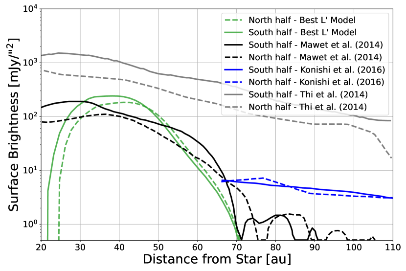
Figure 7: Comparison of our surface brightness measurement (in mJy/(”)²) with literature values in the region around the star between 20 au to 110 au. The dashed green and solid green curves correspond to the north and south region profiles of our best-fit disk model, respectively, measured along the disk major axis using aperture photometry with aperture radii set to $r=\lambda/(2D)\approx 0\hbox{$.\!\!^{\prime\prime}$}06$. The black curves show the published $L^{\prime}$ surface brightness also measured using aperture photometry along the major axis from Mawet et al. (2017). The blue curves show the surface brightness profile measured using broad-band optical imaging from Konishi et al. (2016) and the gray curves illustrate the $8.6\mu$m PAH emission profile from Thi et al. (2014).

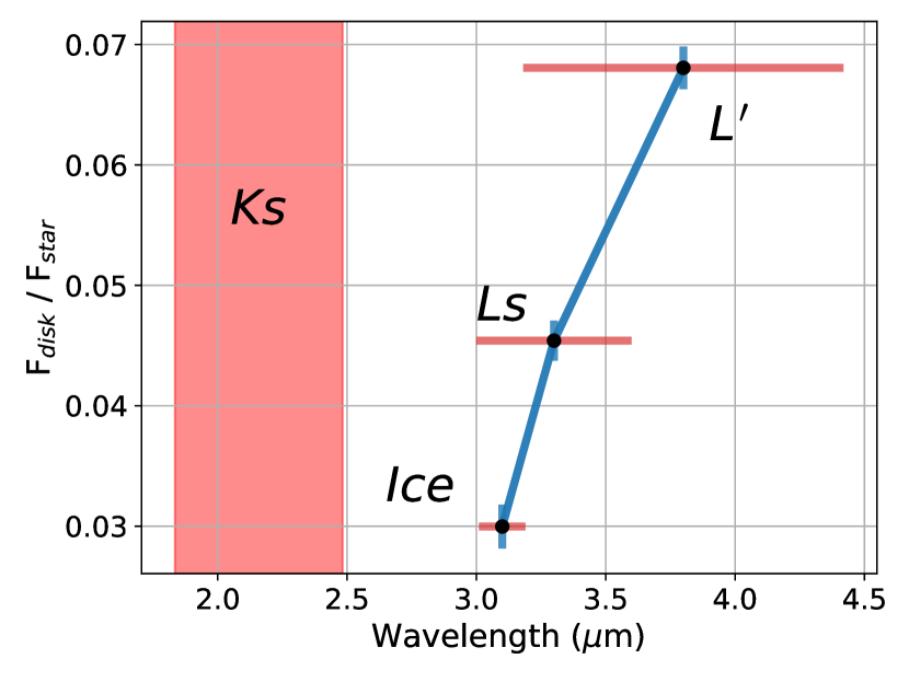
Figure 8: Disk spectrum with respect to the star using our best-fit $L^{\prime}$, $Ls$, and $Ice$ disk models to compute the flux density (see text). The black points denote the disk flux density normalized by the estimated flux density of the star with the vertical blue bars showing the error. The horizontal red lines illustrate the filter bandwidths. We did not detect the disk at $Ks$, but we include the filter bandwidth on the left side of the plot. The flux density decrease from $L^{\prime}$ to $Ice$ bands could indicate absorption of scattered light due to water ice at $3.1\mu$m.

5 Discussion

5.1 Disk Morphology

Our KLIP-RDI images reveal a significant north-south brightness asymmetry in the inner disk, which has also been previously identified (Singh et al. 2021; Bruzzone et al. 2020; Mawet et al. 2017; Perrot et al. 2016); the south half of the disk is brighter. Our model attempts to accommodate this by modifying the sizes of the dust grains to change the amount of forward versus backward scattering of the light and/or altering the irradiance at different regions by applying stellar offsets. We are able to reproduce the observed asymmetry at $L^{\prime}$ and $Ls$ with midplane offsets such that the southwest region of the disk is closest to the star. An eccentric disk could also cause an apparent offset. High eccentricity, (as seen in, e.g., HD 534143; MacGregor et al. 2022) may result from the gravitational influence from nearby or embedded companions. Alternatively, having a higher density of scattering dust in the western half of the disk would make it brighter. The latter notion is consistent with results from Singh et al. (2021), who modeled a higher dust density in the southwest region (roughly $220^{\circ}$ to $238^{\circ}$) to reproduce their polarized intensity images.

The aforementioned brightness asymmetry observed in our $Ice$-band image resulted in a wedged-shaped feature south of the central mask in the S/N of the residuals (bottom right panel of Figure 5; where the S/N peaks at $\sim 3$). To quantify the residual flux, we created a bespoke aperture that was a good match to this feature to measure the residual flux density using the (data - model) image. This procedure yielded about $1.2$ mJy of additional flux density not in the forward model. However, we note that this area is in a region plagued by significant speckle noise in the $L^{\prime}$ and $Ls$ KLIP-RDI images. While we attribute this excess flux to the disk, it is possible that it is just speckle noise.

Our fits to the disk inclination are $\sim 10^{\circ}$ lower than typical literature values (see, e.g., Currie et al. 2016; Perrot et al. 2016; Bruzzone et al. 2020; Singh et al. 2021) though consistent within uncertainties with the results from $L^{\prime}$ image modeling by Mawet et al. (2017). Our model fits may be driven to lower inclination through a combination of factors. First, the noise in the east and west regions close to the star may be underestimated because there are few pixels not containing disk flux with which to measure the noise (see Section 2.2); the zone where $\chi^{2}$ is minimized includes these east-west regions. These minimization zones are illustrated in the third column in Figure 5. Second, as mentioned at the beginning of Section 3, these discrepancies could be a consequence of using a simplistic disk model with some parameters that are not well constrained.

Our KLIP-RDI images at $Ls$ reveal an arc or spiral-like structure at the southeast boundary of the inner disk system; this has been previously noted in the $L^{\prime}$ image studied in (Mawet et al., 2017). Though not explicitly identified, some semblance of this structure is also seen in visible band images (Konishi et al., 2016), and other near-infrared images (Perrot et al., 2016; Currie et al., 2016). Interestingly, our higher quality $Ls$ dataset collected on 2014-Apr-12 (start of night) hints at a point source-like object at the leading tip of the arc or spiral feature, perhaps due to a dust clump. Though this point source-like feature could be the result of the KLIP reduction, we encourage follow-up observations to confirm or rule out this peculiar feature.

The HD 141569A system is well-known for its large two outer rings; the outermost at $\sim 400$ au and the second ring at $\sim 200$ au. These outer disks also have confirmed spiral arms and arcs (e.g., Konishi et al. 2016; Biller et al. 2015), though these outer features curve in the opposing sense to that in the inner region. However, all spiral or arc features currently detected in this system are on the eastern side of the star. The existence of these spirals and arcs perhaps implicate gravitational perturbations either from the two known M dwarf companions or from ongoing planet formation within the disk system.

5.2 Water Ice

We carried out multifilter observations of the inner disk at high S/N at $L^{\prime}$ (3.8 $\mu$m), $Ls$ (3.3 $\mu$m), and narrowband $Ice$ (3.1 $\mu$m). We attempted to observe the disk using a $Ks$ (2.15 $\mu$m) filter, but no disk components were detected in these data. A dip in the brightness of scattered light at $3.1\mu$m should be characteristic of the presence of water ice, as first noted by Inoue et al. (2008). The observed surface brightness in our $Ice$ band KLIP-RDI image might provide clues on the radial distribution of water ice. Figure 6 shows that the $Ice$ KLIP-RDI profile curve for the south disk ansa is comparatively bright closer in towards the star which could be due to a decreasing population of icy grains at smaller stellar distances as seen in HD 100546 (Honda et al., 2009) and AB Aurigae (Betti et al., 2022) (discussed in the following subsection). This same evidence is not seen in the north ansa in our $Ice$ data, however, where the KLIP-RDI image profile indicates that region is dimmer compared to $Ls$ and $L^{\prime}$ at all radial distances. These KLIP-RDI image profiles hint that the disk ansae detected at the $Ice$-band do not scatter less light in comparison to $Ls$ and $L^{\prime}$ until about 40 au (based on this viewing geometry). Nonetheless, considering our extracted surface brightness and total disk flux densities from our modeling (see Section 4.2.3), our results suggest significant absorption due to icy grains at 3.1 $\mu$m.

We only considered silicates in our modeling as we found that constraining an appropriate mix of ice/silicate grains in our scattered light models was difficult, both due to the limited range of scattering angles probed and the limited wavelength range of the data. As such, we leave more concentrated efforts to test mixed grain models to a future study. Despite the absence of a photometric measurement at $Ks$, we do not expect the flux density at this passband to be lower than our $Ice$ measurement. Boccaletti et al. (2003) show that the scattered flux is larger at $1.6\mu$m compared to $2.2\mu$m in the outer two disk components. Moreover, Inoue et al. (2008) show that $K$-band is always brighter relative to $Ice$-band using scattering models. Using our flux density measurements shown in Table 4, we compute a delta magnitude of $(Ice-L^{\prime})=0.51$ mag. Though we lack the $K$-band measurement to directly compare to the color-color diagram in Inoue et al. (2008)’s Figure 5, we expect to be among the optically thin, icy grains classifications.

A simple calculation to get the expected temperature of silicate grains around a star of $T_{\text{eff}}=10000K$ and $L_{\odot}=27.5$ revealed that the water ice sublimation zone terminates at around 6.5 to 12 au depending on the specific grain composition. This is clearly well within our IWA, but one other possibility is that water ice even beyond this estimated sublimation zone is undergoing photodesorption due to UV photons. For disks around Herbig Ae/Be stars, water ice at the surface is expected to have a short lifetime and will readily be destroyed by UV photons (Oka et al., 2012). If we are detecting water ice in the inner disk region of HD 141569A ($\sim 20$ to 70 au) and the disk material is not optically thin to UV flux responsible for quick photodesorption (e.g., Jonkheid et al. 2004), there would need to be some way to explain how the ice is replenished over time. One way ice grains can migrate to the disk surface is through vertical mixing (see, e.g., Takeuchi & Artymowicz 2001), perhaps due to gravitational perturbations on this disk, which is gas-rich (Di Folco et al., 2020).

Detection of water ice has been done using this scattering deficit method for 3 other disk systems: HD 100546 (Honda et al., 2009), HD 142527 (Honda et al., 2016), and AB Aurigae (Betti et al., 2022). We follow with a brief overview of these 3 other icy disk systems.

5.3 Comparing HD 141569 with Other Disks Showing Water Ice Absorption

HD 100546, HD 142527, and AB Aurigae are all Herbig Ae/Be stars (as with HD 141569) whose moderate inclinations allow for comparison of the $\text{H}_{2}$O ice scattering feature in different regions at the disk surface.

5.3.1 Optical Depth Effects

In the case of HD 100546 (Age$\geq 10$ Myr; van den Ancker et al. 1997), Honda et al. (2016) found that the optical depth increases with distance from the star, suggesting a trend of increasing prevalence of icy grains further out from the star which is consistent with our argument presented above. This characteristic was echoed by the recent study of the AB Aurigae system (Age$=4\pm 1$ Myr) by Betti et al. (2022) who also found a lower optical depth at smaller separations from the star, as well as a small asymmetry in optical depth with a higher value along the major axis. However, additional complexity is attributed to the HD 100546 disk considering strong asymmetry found in the absorption feature across the minor axis by Honda et al. (2016) which Tazaki et al. (2021) interpreted as disk subsections possessing higher concentrations of icy grains. Differing optical depths along the major and minor axes were also observed in AB Aurigae by Betti et al. (2022) although the asymmetry was much less pronounced.

5.3.2 Photodesorption

For HD 142527, Honda et al. (2009) performed radiative transfer modeling and concluded that this disk is rather ice rich, with an ice/silicate mass ratio of $\geq 2.2$. However, Tazaki et al. (2021) argued this result to be a consequence of the assumptions made to simplify the modeling such as isotropic scattering. Indeed, as pointed out by Oka et al. (2012), photodesorption of water ice by UV photon exposure at the scattering disk layer makes an ice-heavy composition difficult to maintain. Tazaki et al. (2021) revisited radiative transfer modeling for the HD 142527 disk with added complexity to the scattering and disk geometry assumptions which yielded a lower ice/silicate mass ratio of 0.06 to 0.2 which is consistent with similar modeling efforts for AB Aurigae by Betti et al. (2022) who derived an upper limit on the ice/silicate ratio of $\sim 0.05$. Additionally, Honda et al. (2022) performed a spectropolarimetry analysis on HD 142527 and confirmed the $3.1\mu$m scattering feature in the disk and derived an ice/silicate mass ratio generally consistent with Tazaki et al. (2021). There would be value in similar observations of other Herbig Ae/Be systems since the proximity of these ice/silicate mass ratios begs the question of whether this level of ice composition is a characteristic of them or entirely coincidental.

5.4 Possible Detection of Thermal PAH Emission

We carried out observations at $Ls$ to probe for the $3.3\mu$m PAH emission feature in the HD 141569A disk system and an intriguing result from our forward modeling is the above-mentioned southwestern brightness feature in the best-fit disk models (Figure 5). This brightness enhancement is enigmatic since we assume the east side of the disk is closest to us (see, e.g., Bruzzone et al. 2020) and realistic dust grains tend to forward scatter. One explanation for excess emission from the far side of the disk is PAH emission. This is supported by the brightness of the feature relative to the rest of the disk at $Ls$ when compared to our other models in the adjacent continuum. PAH emission from stochastic, single-photon heating does not have the forward/backward asymmetry that results from scattering (Draine & Li, 2001). PAH emission may be visible in the back scattering regions as well as beyond the peak dust density, providing the PAH grains are illuminated directly by stellar UV and are optically thin to our line of sight.

We attempted a simple experiment to try to constrain the flux density associated with this peculiar brightness feature by generating a $Ls$ disk model with stellar offsets set to zero and subtracting it from the best $Ls$ model displayed in Figure 5. We then integrated the residuals in only this southwest region using an irregular aperture to obtain a flux density estimate of $\sim 2.7$ mJy. Similarly, we repeated these steps, but generated our test model using the parameter solutions for the best $Ice$ model, but retaining the flux scaling parameter for $Ls$ which yielded a flux density estimate of $\sim 4.6$ mJy. Thus if we assume the increase in brightness in the southwestern region is purely due to $3.3\mu$m emission from PAHs, we detect an associated flux density of around 3 – 5 mJy.

We can compare this PAH emission to what might be expected from the disk. First, Geers et al. (2007) found a spectroscopic upper limit to the flux density from $3.3\mu$m PAH emission of $6.9\times 10^{-16}$ W m^-2 for the HD 141569A system. From Castro et al. (2014), we can use a typical line width of $0.03\mu$m for the $3.3\mu$m feature to estimate the total flux density upper limit at 83 mJy. However, we note that this assumes the emitting region was captured within the $0\hbox{$.\!\!^{\prime\prime}$}6$ wide slit used by Geers et al. (2007). Second, the PAH lines at $6.26\mu$m, $7.98\mu$m, and $11.28\mu$m were well-measured in Spitzer spectra (Sloan et al., 2005), with flux ratios reported as $F_{6.2}/F_{7.9}=0.4$ and $F_{11.2}/F_{7.9}=0.04$. We can compare these to the expected flux ratios from PAHs with different sizes and ionization states (Draine et al., 2021). Comparing to Draine et al. (2021)’s Figure 21, HD 141569A has lowest ratios for $F_{6.2}/F_{7.7}=0.28$ and $F_{11.3}/F_{7.7}=0.13$, which indicates small PAHs in a high UV flux. This implies a flux ratio for $F_{3.3}/F_{7.7}$ of 0.1 – 0.2, which in turn gives a flux density prediction of the 3.3 $\mu$m line of 1.7 – $3.4\times 10^{-15}$ W m^-2. We also downloaded a model dust emission spectrum from Draine & Li (2007) corresponding to $U=3\times 10^{5}$, $R_{V}\sim 3.1$ (typical extinction within the Milky Way), and PAH mass fraction $q_{\text{PAH}}=4.48\%$. We subtracted the continuum from small grains before calculating $F_{3.3}/F_{6.6}=0.27$, which then predicts a $3.3\mu$m flux of $1.85\times 10^{-15}$ W m^-2 or 218 mJy using the line width from before. Our estimates are all well below these limits and may point to a stronger PAH abundance interior to our IWA to explain the observationally-inferred value. This idea is supported by the recent detection of a PAH-dominated dusty ring at $\sim 1$ au by GRAVITY (GRAVITY Collaboration et al., 2021).

It has been proposed (Seok & Li 2017, Maaskant et al. 2014, Acke et al. 2010, Keller et al. 2008) that PAHs might trace the geometry of the disk gas. As discussed in Di Folco et al. (2020), the gas around HD 141569A has a flared geometry, which would enable UV photon exposure of the upper disk atmosphere. Additionally, results from Keller et al. (2008) indicate that HD 141569A possesses the most ionized PAH spectrum compared to the other systems surveyed in that study (see their Figure 6). Also suggested in Keller et al. (2008) is the notion that icy mantles on large grains could release PAHs given optical-UV photon exposure, which is consistent with our probable ice detection (see Section 5.2 above). Recent studies using ALMA by Di Folco et al. (2020) and White et al. (2016) found a ¹²CO $J=2\rightarrow 3$ emission asymmetry, with a CO peak in the western region of the disk that is colocated with both the brightness asymmetry we report here as well as the peak dust density region found in Singh et al. (2021). This correspondence between the dust and gas in a restricted location of the disk supports the idea that water ice is resupplied at the surface layer by vertical mixing through drag forces even if the disk is optically thin to the starlight (e.g., Takeuchi & Artymowicz 2001;Lyra & Kuchner 2013). Specifically, collisions between icy planetesimals could release a substantial amount of gas, as has been similarly hypothesized for the $\beta$-Pictoris debris disk (Dent et al., 2014). From the above points, it is possible that our modeling results at $Ls$ and $L^{\prime}$ hint at a complicated spatial distribution of the $3.3\mu$m PAH emission feature. From this, we would also expect a brightness enhancement in the southwestern region in the $Ice$-band image from a deficit of water ice. Figure 5 reveals a significant amount of under-fit flux directly south of the star (bottom right panel), but this location is neither sufficiently far nor close to the peculiar bright region seen in the $Ls$ model to make any definitive conclusions. There would be value in additional observations to test this hypothesis. We encourage more work on constraining the distribution of PAHs in more disk systems to elucidate what exactly they can tell us about the disk environment and ultimately inform us on the stages leading up to early planet formation.

6 Summary & Future Work

We observed HD 141569A using the MagAO+Clio instrument at $L^{\prime}$ ($3.8\mu$m) on UT 2014-04-09, $Ls$ ($3.3\mu$m) on UT 2014-04-11, and narrowband $Ice$ ($3.1\mu$m) on UT 2015-05-29. We performed PSF subtraction using the KLIP-RDI algorithm to detect the inner disk component at S/N of $\sim 10$ at $L^{\prime}$, $\sim 8$ at $Ls$, and $\sim 10$ at $Ice$. We then used our KLIP-RDI images to accomplish simple scattered light disk model fitting using the DiskFM pipeline in pyKLIP. Through our observations we confirmed complex geometrical features such as non-axisymmetric brightness and an arc or spiral feature. We detected a potential point source-like feature at the aforementioned arc’s terminus to which we encourage follow-up observations for confirmation. The best-fit $Ls$ and $L^{\prime}$ models preferentially exhibit peak brightness in the southwest region which could imply the detection of $3.3\mu$m emission due to PAHs. Additionally, a significantly lower surface brightness for our best-fit $Ice$ model compared to our best-fit $L^{\prime}$ model indicates probable detection of water ice in this inner disk region.

Overarching goals for this study included further constraint on the geometrical morphology of the inner disk by forward modeling a simple, scattered light disk model and probing the minimum grain size using a realistic SPF calculated from ADPs (Arnold et al., 2022). Results of these efforts are largely consistent with previous studies with the exception of the disk inclination $i\approx 48^{\circ}$, which is about $10^{\circ}$ less than previous literature values, and a surprisingly high flux from the western half of the disk, despite it being the back-side. One explanation for this western brightness enhancement is the $3.3\mu$m PAH emission feature. This would be co-located with a CO gas enhancement and dust density enhancements seen in other scattered light images (White et al. 2016; Di Folco et al. 2020; Singh et al. 2021). A more complex model is outside the scope of this paper, but may provide answers on which morphological features, if any, are better fit with a combination of scattered light and PAH emission. Furthermore, since our grain size modeling suggests the majority of scattered light detected is from sub-micron grains, it is apparent that the west side of the inner disk presents an ideal opportunity to leverage modeling of the dynamical interactions between the dust and gas, which we encourage as an avenue for future work.

Our analysis of the surface brightness estimates from our best-fitting models suggest significant scattered light absorption at $Ice$ $(3.1\mu$m) perhaps due to icy grains permeating the surface layers of the inner disk. Unfortunately, observations using a bordering $Ks$ filter failed to detect the disk. Additional total intensity observations at $Ks$ or bluer to probe the surface-brightness spectrum are needed to confirm these results and/or characterize the amount of ice. If water ice is present in the upper scattering layers of the inner disk, icy grains would need to be resupplied as their lifetimes in these areas are short due to photodesorption via UV photons exposure. Previously mentioned features such as the spiral or arc-like feature as well as the azimuthal variation of dust and gas hints at gravitational perturbations affecting this inner disk system. To what extent this encourages vertical mixing to cause icy grains to migrate from the midplane to upper disk atmosphere is an analysis saved for a later study.

Appendix A MCMC Modeling Corner Plots

Figures A1, A2, and A3 show corner plots illustrating the output sample posterior distributions from our MCMC runs. The values shown above the histogram plots correspond to those shown in Table 4 . Fitted parameters include the disk critical radius $R_{c}$, inclination $i$, position angle $pa$, x-offset $dx$, y-offset $dy$, a flux scaling parameter $N$, and minimum grain size $a_{\text{min}}$ (see Section 3.1 for further details on the parameters utilized in our modeling). We ran all MCMC runs until the number of iterations exceeded 50 times the maximum autocorrelation time of the walker chains (computed using included functionality of the emcee package; Foreman-Mackey et al. 2013) and discarded the number of initial steps equal twice the autocorrelation time as recommended by the emcee documentation . As a sanity check, visual inspection of the traces of the walker paths showed that the walkers had stabilized well outside of both of these criteria.

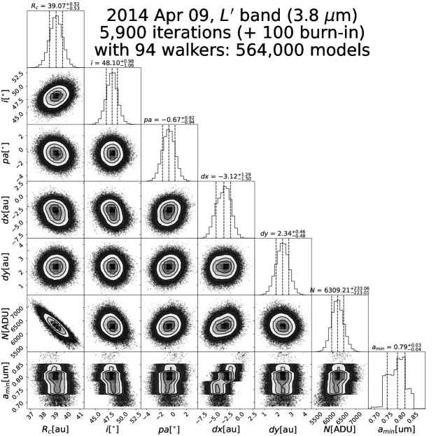
Figure A1: MCMC modeling results using DiskFM for the $L^{\prime}(3.8\mu m)$ band. Histograms on the main diagonal show the posterior probability distributions for each fitted parameter marginalized over all other fitted parameters where the dashed vertical lines show the 16th, 50th, and 84th percentiles. The off-diagonal scatter plots show the joint probability distributions overlaid with contours also representative of the aforementioned percentiles.

References

- Acke et al. (2010) Acke, B., Bouwman, J., Juhász, A., et al. 2010, The Astrophysical Journal, 718, 558, doi: 10.1088/0004-637X/718/1/558
- ALMA Partnership et al. (2015) ALMA Partnership, Brogan, C. L., Pérez, L. M., et al. 2015, The Astrophysical Journall, 808, L3, doi: 10.1088/2041-8205/808/1/L3
- Alvarez & Schuster (1981) Alvarez, M., & Schuster, W. J. 1981, Rev. Mexicana Astron. Astrofis., 6, 163
- Arnold et al. (2022) Arnold, J. A., Weinberger, A. J., Videen, G., & Zubko, E. S. 2022, The Astrophysical Journal, 930, 123, doi: 10.3847/1538-4357/ac63a9
- Augereau et al. (1999) Augereau, J. C., Lagrange, A. M., Mouillet, D., & Ménard, F. 1999, Astronomy & Astrophysics, 350, L51, doi: 10.48550/arXiv.astro-ph/9909423
- Augereau & Papaloizou (2004) Augereau, J. C., & Papaloizou, J. C. B. 2004, Astronomy & Astrophysics, 414, 1153, doi: 10.1051/0004-6361:20031622
- Betti et al. (2022) Betti, S. K., Follette, K., Jorquera, S., et al. 2022, The Astronomical Journal, 163, 145, doi: 10.3847/1538-3881/ac4d9b
- Biller et al. (2015) Biller, B. A., Liu, M. C., Rice, K., et al. 2015, Monthly Notices of the Royal Astronomical Society, 450, 4446, doi: 10.1093/mnras/stv870
- Boccaletti et al. (2003) Boccaletti, A., Augereau, J. C., Marchis, F., & Hahn, J. 2003, ApJ, 585, 494, doi: 10.1086/346019
- Bruzzone et al. (2020) Bruzzone, J. S., Metchev, S., Duchêne, G., et al. 2020, The Astronomical Journal, 159, 53, doi: 10.3847/1538-3881/ab5d2e
- Castro et al. (2014) Castro, A., Miyaji, T., Shirahata, M., et al. 2014, Publications of the Astronomical Society of Japan, 66, 110, doi: 10.1093/pasj/psu096
- Chen et al. (2020) Chen, C., Mazoyer, J., Poteet, C. A., et al. 2020, The Astrophysical Journal, 898, 55, doi: 10.3847/1538-4357/ab9aba
- Clampin et al. (2003) Clampin, M., Krist, J. E., Ardila, D. R., et al. 2003, The Astronomical Journal, 126, 385, doi: 10.1086/375460
- Currie et al. (2016) Currie, T., Grady, C. A., Cloutier, R., et al. 2016, The Astrophysical Journal, 819, L26, doi: 10.3847/2041-8205/819/2/L26
- Cutri et al. (2014) Cutri, R. M., Wright, E. L., Conrow, T., et al. 2014, Vizier Online Data Catalog, 2328, 0
- Dent et al. (2014) Dent, W. R. F., Wyatt, M. C., Roberge, A., et al. 2014, Science, 343, 1490, doi: 10.1126/science.1248726
- Di Folco et al. (2020) Di Folco, E., Péricaud, J., Dutrey, A., et al. 2020, Astronomy & Astrophysics, 635, A94, doi: 10.1051/0004-6361/201732243
- Draine (2003a) Draine, B. T. 2003a, The Astrophysical Journal, 598, 1017, doi: 10.1086/379118
- Draine (2003b) —. 2003b, The Astrophysical Journal, 598, 1026, doi: 10.1086/379123
- Draine & Li (2001) Draine, B. T., & Li, A. 2001, The Astrophysical Journal, 551, 807, doi: 10.1086/320227
- Draine & Li (2007) —. 2007, The Astrophysical Journal, 657, 810, doi: 10.1086/511055
- Draine et al. (2021) Draine, B. T., Li, A., Hensley, B. S., et al. 2021, The Astrophysical Journal, 917, 3, doi: 10.3847/1538-4357/abff51
- Foreman-Mackey et al. (2013) Foreman-Mackey, D., Hogg, D. W., Lang, D., & Goodman, J. 2013, PASP, 125, 306, doi: 10.1086/670067
- Gaia Collaboration et al. (2023) Gaia Collaboration, Vallenari, A., Brown, A. G. A., et al. 2023, Astronomy & Astrophysics, 674, A1, doi: 10.1051/0004-6361/202243940
- Gáspár et al. (2023) Gáspár, A., Wolff, S. G., Rieke, G. H., et al. 2023, Nature Astronomy, 7, 790, doi: 10.1038/s41550-023-01962-6
- Geers et al. (2007) Geers, V. C., van Dishoeck, E. F., Visser, R., et al. 2007, Astronomy & Astrophysics, 476, 279, doi: 10.1051/0004-6361:20078466
- GRAVITY Collaboration et al. (2021) GRAVITY Collaboration, Ganci, V., Labadie, L., et al. 2021, Astronomy & Astrophysics, 655, A112, doi: 10.1051/0004-6361/202141103
- Guizar-Sicairos et al. (2008) Guizar-Sicairos, M., Thurman, S. T., & Fienup, J. R. 2008, Optics Letters, 33, 156, doi: 10.1364/OL.33.000156
- Høg et al. (2000) Høg, E., Fabricius, C., Makarov, V. V., et al. 2000, Astronomy & Astrophysics, 355, L27
- Honda et al. (2009) Honda, M., Inoue, A. K., Fukagawa, M., et al. 2009, The Astrophysical Journall, 690, L110, doi: 10.1088/0004-637X/690/2/L110
- Honda et al. (2016) Honda, M., Kudo, T., Takatsuki, S., et al. 2016, The Astrophysical Journal, 821, 2, doi: 10.3847/0004-637X/821/1/2
- Honda et al. (2022) Honda, M., Tazaki, R., Murakawa, K., et al. 2022, Publications of the Astronomical Society of Japan, 74, 851, doi: 10.1093/pasj/psac041
- Inoue et al. (2008) Inoue, A. K., Honda, M., Nakamoto, T., & Oka, A. 2008, Publications of the Astronomical Society of Japan, 60, 557, doi: 10.1093/pasj/60.3.557
- Jonkheid et al. (2004) Jonkheid, B., Faas, F. G. A., van Zadelhoff, G. J., & van Dishoeck, E. F. 2004, A&A, 428, 511, doi: 10.1051/0004-6361:20048013
- Jonkheid et al. (2006) Jonkheid, B., Kamp, I., Augereau, J. C., & van Dishoeck, E. F. 2006, Astronomy & Astrophysics, 453, 163, doi: 10.1051/0004-6361:20054769
- Keller et al. (2008) Keller, L. D., Sloan, G. C., Forrest, W. J., et al. 2008, The Astrophysical Journal, 684, 411, doi: 10.1086/589818
- Konishi et al. (2016) Konishi, M., Grady, C. A., Schneider, G., et al. 2016, The Astrophysical Journal, 818, L23, doi: 10.3847/2041-8205/818/2/L23
- Lawson et al. (2020) Lawson, K., Currie, T., Wisniewski, J. P., et al. 2020, The Astronomical Journal, 160, 163, doi: 10.3847/1538-3881/ababa6
- Lyra & Kuchner (2013) Lyra, W., & Kuchner, M. 2013, Nature, 499, 184, doi: 10.1038/nature12281
- Maaskant et al. (2014) Maaskant, K. M., Min, M., Waters, L. B. F. M., & Tielens, A. G. G. M. 2014, Astronomy & Astrophysics, 563, A78. https://ui.adsabs.harvard.edu/abs/2014A&A...563A..78M
- MacGregor et al. (2022) MacGregor, M. A., Hurt, S. A., Stark, C. C., et al. 2022, The Astrophysical Journall, 933, L1, doi: 10.3847/2041-8213/ac7729
- Mawet et al. (2017) Mawet, D., Choquet, E., Absil, O., et al. 2017, The Astronomical Journal, 153, 44, doi: 10.3847/1538-3881/153/1/44
- Mazoyer et al. (2020) Mazoyer, J., Arriaga, P., Hom, J., et al. 2020, Proc. SPIE, 11447, 1144759, doi: 10.1117/12.2560091
- Merín et al. (2004) Merín, B., Montesinos, B., Eiroa, C., et al. 2004, Astronomy & Astrophysics, 419, 301, doi: 10.1051/0004-6361:20034561
- Millar-Blanchaer et al. (2015) Millar-Blanchaer, M. A., Graham, J. R., Pueyo, L., et al. 2015, The Astrophysical Journal, 811, 18, doi: 10.1088/0004-637X/811/1/18
- Milli et al. (2012) Milli, J., Mouillet, D., Lagrange, A. M., et al. 2012, Astronomy & Astrophysics, 545, A111, doi: 10.1051/0004-6361/201219687
- Morzinski et al. (2015) Morzinski, K. M., Males, J. R., Skemer, A. J., et al. 2015, The Astrophysical Journal, 815, 108, doi: 10.1088/0004-637X/815/2/108
- Morzinski et al. (2016) Morzinski, K. M., Close, L. M., Males, J. R., et al. 2016, in Society of Photo-Optical Instrumentation Engineers (SPIE) Conference Series, Vol. 9909, Adaptive Optics Systems V, ed. E. Marchetti, L. M. Close, & J.-P. Véran, 990901, doi: 10.1117/12.2233911
- Mouillet et al. (2001) Mouillet, D., Lagrange, A. M., Augereau, J. C., & Ménard, F. 2001, Astronomy & Astrophysics, 372, L61, doi: 10.1051/0004-6361:20010660
- Oka et al. (2012) Oka, A., Inoue, A. K., Nakamoto, T., & Honda, M. 2012, The Astrophysical Journal, 747, 138, doi: 10.1088/0004-637X/747/2/138
- Perrot et al. (2016) Perrot, C., Boccaletti, A., Pantin, E., et al. 2016, Astronomy & Astrophysics, 590, L7, doi: 10.1051/0004-6361/201628396
- Pueyo (2016) Pueyo, L. 2016, The Astrophysical Journal, 824, 117, doi: 10.3847/0004-637X/824/2/117
- Reche et al. (2009) Reche, R., Beust, H., & Augereau, J.-C. 2009, Astronomy & Astrophysics, 493, 661, doi: 10.1051/0004-6361:200810419
- Ren et al. (2019) Ren, B., Choquet, É., Perrin, M. D., et al. 2019, The Astrophysical Journal, 882, 64, doi: 10.3847/1538-4357/ab3403
- Ruane et al. (2019) Ruane, G., Ngo, H., Mawet, D., et al. 2019, The Astronomical Journal, 157, 118, doi: 10.3847/1538-3881/aafee2
- Seok & Li (2017) Seok, J. Y., & Li, A. 2017, The Astrophysical Journal, 835, 291, doi: 10.3847/1538-4357/835/2/291
- Shahar et al. (2019) Shahar, A., Driscoll, P., Weinberger, A., & Cody, G. 2019, Science, 364, 434. https://ui.adsabs.harvard.edu/abs/2019Sci...364..434S
- Siebenmorgen & Heymann (2012) Siebenmorgen, R., & Heymann, F. 2012, Astronomy & Astrophysics, 543, A25, doi: 10.1051/0004-6361/201219039
- Singh et al. (2021) Singh, G., Bhowmik, T., Boccaletti, A., et al. 2021, Astronomy & Astrophysics, 653, A79, doi: 10.1051/0004-6361/202140319
- Skrutskie et al. (2006) Skrutskie, M. F., Cutri, R. M., Stiening, R., et al. 2006, The Astronomical Journal, 131, 1163, doi: 10.1086/498708
- Sloan et al. (2005) Sloan, G. C., Keller, L. D., Forrest, W. J., et al. 2005, The Astrophysical Journal, 632, 956, doi: 10.1086/444371
- Soummer et al. (2012) Soummer, R., Pueyo, L., & Larkin, J. 2012, The Astrophysical Journal, 755, L28, doi: 10.1088/2041-8205/755/2/L28
- Soummer et al. (2014) Soummer, R., Perrin, M. D., Pueyo, L., et al. 2014, The Astrophysical Journall, 786, L23, doi: 10.1088/2041-8205/786/2/L23
- Takeuchi & Artymowicz (2001) Takeuchi, T., & Artymowicz, P. 2001, ApJ, 557, 990, doi: 10.1086/322252
- Tazaki et al. (2021) Tazaki, R., Murakawa, K., Muto, T., Honda, M., & Inoue, A. K. 2021, The Astrophysical Journal, 921, 173, doi: 10.3847/1538-4357/ac1f8c
- Thi et al. (2014) Thi, W.-F., Pinte, C., Pantin, E., et al. 2014, Astronomy & Astrophysics, 561, A50, doi: 10.1051/0004-6361/201322150
- Tielens (2008) Tielens, A. G. G. M. 2008, ARA&A, 46, 289, doi: 10.1146/annurev.astro.46.060407.145211
- van den Ancker et al. (1997) van den Ancker, M. E., The, P. S., Tjin A Djie, H. R. E., et al. 1997, Astronomy & Astrophysics, 324, L33
- Wang et al. (2015) Wang, J. J., Ruffio, J.-B., De Rosa, R. J., et al. 2015, pyKLIP: PSF Subtraction for Exoplanets and Disks (Astrophysics Source Code Library), ascl:1506.001. http://ascl.net/1506.001
- Weinberger et al. (1999) Weinberger, A. J., Becklin, E. E., Schneider, G., et al. 1999, The Astrophysical Journal, 525, L53, doi: 10.1086/312334
- Weinberger et al. (2000) Weinberger, A. J., Rich, R. M., Becklin, E. E., Zuckerman, B., & Matthews, K. 2000, The Astrophysical Journal, 544, 937, doi: 10.1086/317243
- White et al. (2016) White, J. A., Boley, A. C., Hughes, A. M., et al. 2016, The Astrophysical Journal, 829, 6, doi: 10.3847/0004-637X/829/1/6
- Wyatt (2005) Wyatt, M. C. 2005, Astronomy & Astrophysics, 440, 937, doi: 10.1051/0004-6361:20053391
- Wyatt et al. (2015) Wyatt, M. C., Panić, O., Kennedy, G. M., & Matrà, L. 2015, Astrophysics and Space Science, 357, 103, doi: 10.1007/s10509-015-2315-6
- Zubko et al. (2015) Zubko, E., Shkuratov, Y., & Videen, G. 2015, Journal of Quantitative Spectroscopy and Radiative Transfer, 150, 42, doi: 10.1016/j.jqsrt.2014.06.023
- Zuckerman et al. (1995) Zuckerman, B., Forveille, T., & Kastner, J. H. 1995, Nature, 373, 494, doi: 10.1038/373494a0