Data-Driven Modeling and Verification of Perception-Based Autonomous Systems

Abstract

This paper addresses the problem of data-driven modeling and verification of perception-based autonomous systems. We assume the perception model can be decomposed into a canonical model (obtained from first principles or a simulator) and a noise model that contains the measurement noise introduced by the real environment. We focus on two types of noise, benign and adversarial noise, and develop a data-driven model for each type using generative models and classifiers, respectively. We show that the trained models perform well according to a variety of evaluation metrics based on downstream tasks such as state estimation and control. Finally, we verify the safety of two systems with high-dimensional data-driven models, namely an image-based version of mountain car (a reinforcement learning benchmark) as well as the F1/10 car, which uses LiDAR measurements to navigate a racing track.

1 Introduction

From self-driving cars ([waymo]) to taxi helicopters ([volocity]), the last few years have seen the development of a number of impressive autonomous systems. As the complexity of these systems increases, however, so does the concern for their safety. In fact, we have already witnessed accidents involving systems as diverse as autonomous cars (e.g., see the reports by the [tesla_report] and the [uber_report]), chess-playing robots (as reported by [chess_robot]) and autonomous aircraft (analyzed in an [boeing_report] report). Furthermore, the United States government recently recorded 367 crashes involving autonomous cars over a 10-month period ([nhtsa]). In order to prevent such incidents, it is essential that we verify the safety of autonomous systems before they are deployed in the wild.

Unlike classical control systems, modern autonomous systems introduce an extra layer of complexity since they operate in complex environments, which are perceived through high-dimensional measurements such as LiDAR scans and camera images. In turn, these measurements are processed by neural networks (NNs) used for estimation and control. Verifying such a closed-loop system at design-time poses two significant challenges: 1) environment models are difficult to develop from first principles due to unexpected noise, e.g., reflected LiDAR rays ([ivanov20a]); 2) NNs are not robust to even small input perturbations ([szegedy13]) and distribution shifts ([recht19]), which may reduce the utility of verification performed against an imperfect model.

To overcome these challenges, in this paper we propose a compositional verification approach that uses data-driven environment models. We compose two types of models: 1) a canonical environment model (e.g., during daytime with perfect visibility) that is obtained from first principles or through a simulator; 2) a data-driven noise model that is trained on real data to augment the canonical model with data artifacts observed during real system operation (e.g., blurred images or reflected LiDAR rays). This approach is motivated by recent work by [katz22] on developing (and verifying) canonical models from real observations as well as work by [wu23] on using generative models for certifying the robustness of NNs to real-world distribution shifts. The compositional model has several benefits over a single monolithic model: 1) the canonical model need not be data-driven, thereby reducing the data requirements for training the perception model; 2) different noise models can be composed with the canonical model to capture diverse scenarios; 3) individual noise models can be smaller, thereby alleviating verification scalability challenges.

Training noise models presents an interesting challenge since some types of noise are easier to capture using generative models than other types. For example, continuous noise (e.g., blur or contrast) is fairly benign and is easily learned by a generative model. However, discontinuous noise (e.g., reflected LiDAR rays or lens flare) is more adversarial and cannot be perfectly learned using a continuous model. We handle these two cases separately: 1) for benign noise, we use generative models, e.g., variational autoencoders as introduced by [kingma13]; 2) for adversarial noise (defined as high-frequency large deviation from the canonical model), we train classifiers that indicate which part of the canonical measurement is affected and can be replaced with the effect of the adversarial noise. In fact, our experiments suggest that it is exactly the discontinuous noise that causes the largest deviations in control performance as compared to the canonical environment.

To evaluate the compositional data-driven modeling approach, we present two verification case studies: 1) Mountain Car (MC), which is a reinforcement learning (RL) benchmark available in [mc]; 2) the [f1tenth], which is a 1/10-scale autonomous racing car platform. In MC, we train an image-based control pipeline and verify that the car reaches the goal for a range of benign noises, including blur and contrast. In the F1/10 case, we use existing LiDAR traces ([ivanov20a]) to train an adversarial noise classifier. The noise model’s quality is evaluated on the downstream control task, by comparing the control output on real vs. modeled LiDAR scans. Finally, we verify that the F1/10 car, coupled with a robust denoiser, can safely navigate an environment under adversarial LiDAR noise that was shown to be correlated with crashes by [ivanov20a]. In both cases, we performed the verification using our tool, Verisig ([ivanov19, ivanov20, ivanov2021b]).

In summary, the contributions of this paper are as follows: 1) a compositional data-driven method for developing perception models used in verification; 2) a noise-specific approach that uses generative models for benign noise and classifiers for adversarial noise; 3) two verification case studies illustrating the benefit of data-driven modeling and verification.

Related work.

Verification of standard (non-neural) control systems is a mature field. A classical approach to reachability is by using Hamilton-Jacobi methods ([mitchell02, chen18]). Another class of techniques approximate reachable sets using Taylor models ([makino03, chen12], ellipsoids ([althoff15]), and polytopes ([chutinan03]). Finally, there also exist methods that cast the problem as a satisfiability modulo theory program ([gao13, kong15]). More recently, a number of works were developed for open-loop verification of NNs, such as input-output robustness, e.g., works by [dutta18, ehlers17, fazlyab19, gehr18, katz17, wang18, weng18, tran20, wang21]. Methods also exist for verification of closed-loop systems with NN components such as those by [ivanov19, huang19, dutta19, sun19, tran19, bogomolov19, dreossi19].

For systems with high-dimensional perception, [katz22] developed a verification method by training a generative image model using simulated data. [ivanov20a] used a first-principles LiDAR model to verify the safety of the F1/10 car as it navigates a racing track. [hsieh22] verified perception-based systems using approximate abstractions of the perception system. Although these works are good first steps, they do not account for the distribution shift between the canonical model and the real data that would be captured by our noise model. Approaches also exist ([dawson22, robey20, robey21b]) for learning safe barrier certificates from images but these do not provide worst-case guarantees on the learned certificate. Finally, a number of works exist ([hanspal23, robey2020model, wu23]) that use model-based generative NNs for open-loop verification and robustness purposes; we borrow ideas from these approaches (e.g., model-based training) when tackling the closed-loop problem.

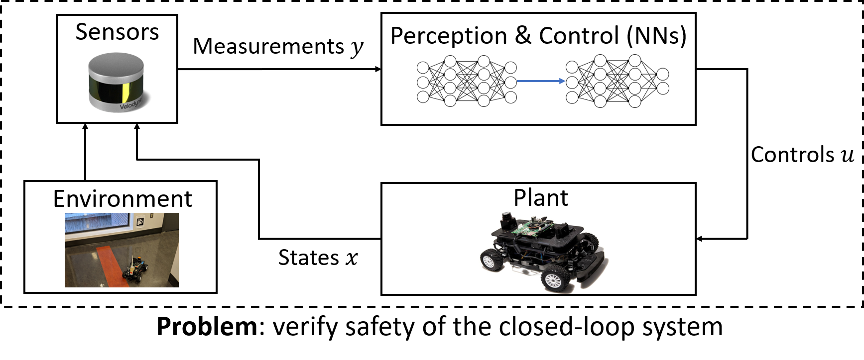
Figure 1: Overview of the problem considered in this paper.

2 Problem Formulation

This section formalizes the problem addressed in this paper. We consider a closed-loop autonomous system, as illustrated in Figure 1. Formally, we are given a dynamical system of the sort:

$$\begin{split}x_{k+1}&=f(x_{k},u_{k})\\ y_{k}&=g(x_{k})=g_{n}(x_{k},\delta_{k})\circ g_{c}(x_{k})\\ u_{k}&=h(y_{k}),\end{split}$$ (1)

where $x\in\mathbb{R}^{n}$ is the system state (e.g., position, velocity), $y\in\mathbb{R}^{m}$ are the measurements (e.g., camera images and LiDAR scans) and $u\in\mathbb{R}^{p}$ are the controls. The dynamics $f$ are known. The observation model $g$ is unknown but we assume it can be represented as the composition of a canonical environment model, $g_{c}$, and a noiser, $g_{n}$. The canonical model is known (either developed from first principles or a simulator); the noiser is unknown as it contains the noise profile of the real environment the system operates in; the parameter $\delta_{k}$ specifies the noise intensity (e.g., blur level). Finally, $h$ encodes the perception/control pipeline and contains one or more NNs.

To train the noise model, we assume we are given a training set $\mathcal{D}=\{(x_{i},y_{i})\}$ of states and measurements. The training set is collected by running the system (e.g., manually) in the real environment. This setting is inspired by the one considered by [dean20], where $\mathcal{D}$ is used to obtain probably approximately correct (PAC) bounds on perception error. An important challenge is developing a metric for evaluating the noise model’s quality; metrics defined on the high-dimensional measurement space may be misleading, as distances (e.g., pixel differences) may not be semantically meaningful. Thus, part of the problem is to develop a semantically meaningful metric to evaluate the noise model. We now state the two problems considered in this work.

Problem 1

Consider the closed-loop system in eq:system_model. Given a training dataset, $\mathcal{D}=\{(x_{i},y_{i})\}$, train a noise model, $g_{n}$. Furthermore, develop a semantically meaningful evaluation metric for $g_{n}$.

Problem 2

Consider the closed-loop system in eq:system_model where $g_{n}$ is well trained. Given an initial set $\mathcal{X}_{0}$, the problem is to verify a safety property $\phi$ (e.g., no collisions) of the reachable states $x_{k}$:

$$(x_{0}\in\mathcal{X}_{0})\Rightarrow\phi(x_{k}),\ \forall k\geq 0.$$ (2)

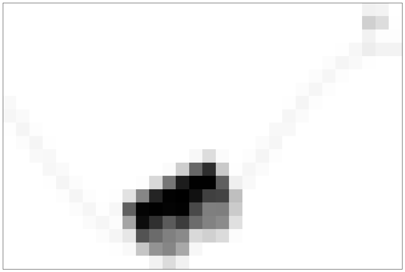
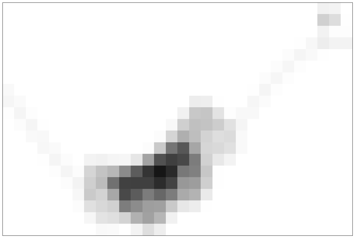
fig:mc_examples [Canonical][b] [Reduced Contrast][b] [Blur][b] [Contrast + Blur][b]

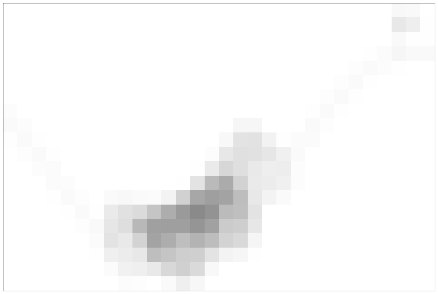
Figure 2: Examples of benign noise in the MC environment.

3 Motivating Examples

This section presents two examples to illustrate different system setups, i.e., an image-based vs. a LiDAR-based system, as well as different noise types, namely benign vs. adversarial. Finally, while the MC example is purely synthetic, the F1/10 case study uses real data to train the noise model.

3.1 Mountain Car: An Image-Based System Operating Under Benign Noise

MC is an RL benchmark where the task is to drive an underpowered car up a hill, as illustrated in Figure 2 (we modified the environment by reducing the image size and making the car bigger). Since the car does not have enough power, it needs to learn to drive up the left hill so as to gather momentum and get to the goal on the right. MC consists of two states, position and velocity, which are both observed by the controller in the original MC environment. In this paper, we consider the case where the controller observes an image (such as the one in Figure 2), coupled with velocity.

Given an image-based controller, we are interested in verifying the system’s robustness to environment noise. As illustrated in Figures 2 and 2, we consider two types of noise, contrast and blur (as well as their combination, shown in Figure 2), that aim to capture realistic operating conditions. Different contrast corresponds to changing lighting conditions, e.g., time of day, whereas blur occurs at higher driving speeds. Both noise types are continuous and are classified as benign. Section 4 presents a method to train and verify a generative model for such types of noise.

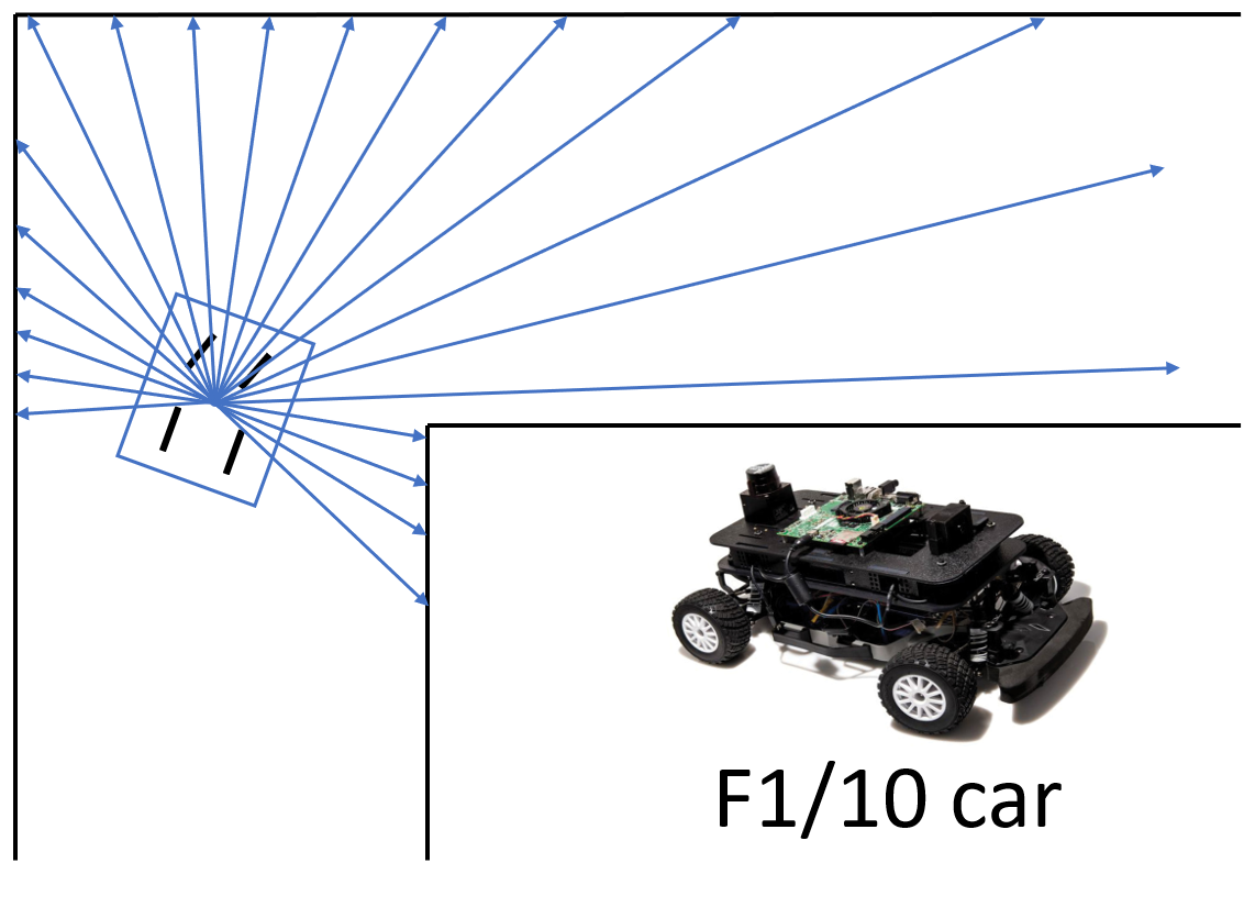
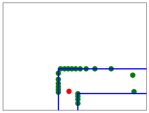
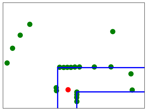
fig:f11_examples [LiDAR illustration][b] [Canonical scan at $x_{k}$][b] [Real scan at $x_{k}$][b] [Real scan at $x_{k+1}$][b]

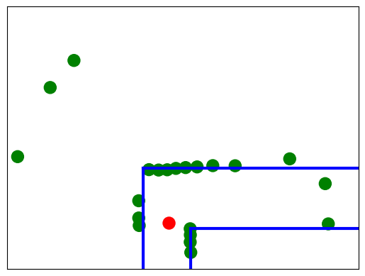
Figure 3: Illustration of the F1/10 car, including canonical and real scans featuring adversarial noise.

3.2 The F1/10 Car: A LiDAR-Based System Operating Under Adversarial Noise

The [f1tenth] is a popular autonomous racing platform. It exhibits a number of the challenges introduced by full scale autonomous cars, such as noisy measurements, adversarial agents, and fast-paced environments. We focus on the case of a single car navigating a square track using LiDAR measurements, as shown in Figure 3. In prior work, [ivanov20a] used RL to train a number of controllers in a simulated environment and subsequently verified that these controllers are safe in the simulated environment. However, [ivanov20a] also demonstrated that the controllers resulted in a number of accidents in the real world, as caused by noisy real data.

A canonical 21-dimensional LiDAR scan for a right-hand turn is illustrated in Figure 3. Figures 3 and 3 show noisy real scans collected by [ivanov20a] in a real environment similar to the simulated one; the car pose is the same (up to estimation error) in both environments. The real data contains reflected LiDAR rays (e.g., due to metallic surfaces), which manifest as perceived gaps in the environment. Such patterns are discontinuous and are classified as adversarial. Indeed, [ivanov20a] showed that the number of accidents is significantly reduced if reflected surfaces are covered, thereby confirming the adversarial nature of LiDAR noise. Section 4 presents a classifier-based approach for modeling adversarial noise for verification purposes.

4 Modeling Framework

This section presents our modeling framework, including the canonical environment model and the two types of noise models. We also present a method for evaluating the quality of these components.

4.1 Canonical Model

We focus on static environments where a first-principles model can describe the main features but may fail to capture environmental noise such as reflective surfaces and changing lighting conditions. Building a (canonical) first-principles model is particularly useful in such a setting as it enables the development of controllers in simulation. Once such a controller is built, deploying the system in the real environment requires only a “de-noiser” for that specific environment, i.e., an additional component that is trained to translate real measurements to canonical ones. Thus, canonical models are by definition modular – the same canonical model can be be composed with different noiser/de-noiser settings and can thus be used for different environments that are the same up to measurement noise (e.g., roads with various degrees of marking degradation). In future work, we will also consider the case where the canonical model is augmented with other agents observed in the real environment.

4.2 Noise Model

When developing a noise model for the purposes of verification, there are two main scalability-related requirements: 1) models should be small and modular; 2) models should not introduce significant spurious (unrealistic) noise, as that greatly complicates the verification task. Training a single model that satisfies both of these requirements is challenging, especially when one considers the types of noise illustrated in Section 3. In particular, such a model would be exceedingly large for verification purposes and would likely introduce a large number of spurious behaviors in order to capture discontinuous noise (NNs are by definition continuous, so the only way to capture discontinuous dynamics is through including all in-between values as well). Thus, we argue that it is necessary to train a separate noise model for each type of noise. In what follows, we define each type of noise formally and describe a training procedure for the corresponding noise model.

Benign Noise.

Intuitively, benign noise is noise that is easy to learn, both to generate and to be robust to. In their seminal paper, [szegedy13] show that NN classifiers are robust to Gaussian noise, even if the noise results in more distorted images than adversarial noise. We observe a similar pattern in the context of the examples considered in this paper: continuous/benign noise is easier to learn than discontinuous/adversarial noise. Formally, we define benign noise as follows.

Definition 4.1 (Benign Noise).

Let $\Delta_{x}=g_{n}(x,g_{c}(x),\delta)-g_{c}(x)$ be the measurement noise introduced by the environment. We classify $\Delta_{x}$ as benign if it changes slowly across the state space $\mathcal{X}$:

$$\forall\varepsilon_{x}>0\ \exists\varepsilon_{\Delta}>0\text{s.t.}\forall x,x^{\prime}\in\mathcal{X},\ \|x-x^{\prime}\|_{\infty}\leq\varepsilon_{x}\Rightarrow\|\Delta_{x}-\Delta_{x^{\prime}}\|_{\infty}\leq\varepsilon_{\Delta}.$$

Definition 4.1 captures not only noise that is small in magnitude, but also noise that may be large in magnitude but is not changing across the state-space (e.g., a change in lighting conditions may result in large noise overall but is easy to learn as it is reasonably constant). This definition captures both types of noise considered in the MC case study, which introduce significant changes to the canonical image but are consistent across states. To train a generative model for benign noise given a training set ${\mathcal{D}=\{(x_{i},y_{i})\}}$, one can use a number of losses, e.g., mean squared error, binary cross entropy (BCE), or reconstruction loss as introduced by [kingma13]. In the experiments, we use BCE with fully-connected NN models as this is the NN architecture supported by Verisig.

Adversarial Noise.

Adversarial noise is high-frequency noise that may change quickly across the state space, as demonstrated in Figures 3 and 3. For example, LiDAR rays are always reflected be some surfaces (or may be reflected by other surfaces only under certain angles). Such noise is similar to the adversarial noise for classification tasks discovered by [szegedy13].

Definition 4.2 (Adversarial Noise.).

We classify $\Delta_{x}$ (introduced in Definition 4.1) as adversarial noise if there exists a subset $\mathcal{X}_{a}\subseteq\mathcal{X}$ such that $\forall x\in\mathcal{X},\forall x_{a}\in\mathcal{X}_{a},\ \|\Delta_{x}-\Delta_{x_{a}}\|_{\infty}>\varepsilon_{a}$ for some $\varepsilon_{a}>0$.

As argued above, training a generative model for adversarial noise is challenging since we are effectively trying to capture a discontinuous space using a continuous model. Thus, we propose to use a classifier, $c_{n}:\mathcal{X}\times\mathcal{Y}\to\{0,1\}^{m}$, that determines whether a measurement (dimension) is corrupted by adversarial noise. If a certain dimension is flagged, then its value is reset to a default value, $y_{a}$, corresponding to the effect of that type of noise (e.g., reflected LiDAR rays are set to the maximum LiDAR range whereas pixels affected by glare can be reset to white). Formally,