Spectral State Space Models

Abstract

This paper studies sequence modeling for prediction tasks with long range dependencies. We propose a new formulation for state space models (SSMs) based on learning linear dynamical systems with the spectral filtering algorithm (Hazan et al., 2017). This gives rise to a novel sequence prediction architecture we call a spectral state space model.

Spectral state space models have two primary advantages. First, they have provable robustness properties as their performance depends on neither the spectrum of the underlying dynamics nor the dimensionality of the problem. Second, these models are constructed with fixed convolutional filters that do not require learning while still outperforming SSMs in both theory and practice.

The resulting models are evaluated on synthetic dynamical systems and long-range prediction tasks of various modalities. These evaluations support the theoretical benefits of spectral filtering for tasks requiring very long range memory.

1 Introduction

Handling long-range dependencies efficiently remains a core problems in sequence prediction/modelling. Recurrent Neural Networks (Hopfield, 1982; Rumelhart et al., 1985; Elman, 1990) are a natural choice for sequence modelling, but are notoriously hard to train; they often suffer from vanishing and exploding gradients (Bengio et al., 1994; Pascanu et al., 2013) and despite techniques to mitigate the issue (Hochreiter & Schmidhuber, 1997; Cho et al., 2014; Arjovsky et al., 2016), they are also hard to scale given the inherently sequential nature of their computation.

In recent years, transformer models (Vaswani et al., 2017) have become the staple of sequence modelling, achieving remarkable success across multiple domains (Brown et al., 2020; Dosovitskiy et al., 2020; Jumper et al., 2021). Transformer models are naturally parallelizable and hence scale significantly better than RNNs. However, the attention layers have memory and computation requirements that scale quadratically with context length. Many approximations to the standard attention layers have been proposed (see (Tay et al., 2022) for a recent survey).

Recurrent Neural Networks have seen a recent resurgence in the form of state space models (SSM) which have shown promise modelling long-range sequences across varied modalities (Gu et al., 2021a; Dao et al., 2022; Gupta et al., 2022; Orvieto et al., 2023; Poli et al., 2023; Gu & Dao, 2023). SSMs use linear dynamical systems (LDS) to model the sequence-to sequence transform by evolving the internal state of a dynamical system according to the dynamics equations

$$x_{t}=Ax_{t-1}+Bu_{t}$$

$$y_{t}=Cx_{t}+Du_{t}.$$

Here $x_{t}\in{\mathbb{R}}^{d}$ is the hidden state of the dynamical system, $u_{t}$ is the input to the system, and $y_{t}$ are observations. The matrices $A,B,C,D$ govern the evolution of the system and are called system matrices. Despite its simplicity, this linear model can capture a rich set of natural dynamical systems in engineering and the physical sciences due to the potentially large number of hidden dimensions. Linear dynamical systems are also attractive as a sequence model because their structure is amenable to both fast inference and fast training via parallel scans (Blelloch, 1989; Smith et al., 2023) or convolutions (Gu et al., 2021a). A rich literature stemming from control theory and recent machine learning interest has given rise to efficient techniques for system identification, filtering, and prediction for linear dynamical systems. For a survey of recent literature see Hazan & Singh (2022).

These techniques make SSMs attractive for sequence tasks which inherently depend on long contexts that scale poorly for transformers. Examples include large language models (Dao et al., 2022), modelling time series (Zhang et al., 2023), and audio generation (Goel et al., 2022). To understand the factors affecting the memory in an SSM or simply a linear dynamical system, we now proceed to delineate how past states and inputs affect the future.

Geometric decay in LDS.

The linear equations governing the dynamics are recursive in nature, and imply that in a noiseless environment, the $t$’th observation can be written as

$$y_{t}=Cx_{t}+Du_{t} =C(Ax_{t-1}+Bu_{t})+Du_{t}=...$$

$$=\sum_{i=0}^{t-1}CA^{i}Bu_{t-i}+Du_{t}$$

The matrix $A$ is asymmetric in general, and can have complex eigenvalues. If the amplitude of these eigenvalues is larger than one, then the the observation $y_{t}$ can grow without bounds. This is called an “explosive” system. In a well-behaved system, the eigenvalues of $A$ have magnitude smaller than one. If the magnitudes are bounded away from one, say $|\lambda_{i}(A)|<1-\delta$, for some small $\delta>0$, then we can write

$$y_{t}=\sum_{i=0}^{k}CA^{i}Bu_{t-i}+\omega_{k}\ \ ,\ \ \|\omega_{k}\|\leq\varepsilon$$

for $k=O(\frac{1}{\delta}\log\frac{1}{\varepsilon})$. This mathematical fact implies that the effective memory of the system is on the order of $\frac{1}{\delta}$. In general, the parameter $\delta$ is unknown apriori and can get arbitrarily small as we approach systems with have long range dependencies leading to instability in training linear dynamical systems with a long context. This issue is specifically highlighted in the work of Orvieto et al. (2023) who observe that on long range tasks learning an LDS directly does not succeed and requires interventions such as stable exponential parameterizations and specific normalization which have been repeatedly used either implicitly or explicitly in the SSM literature (Gu et al., 2021a). Unfortunately these reparametrizations and normalizations come with no theoretical guarantees. In fact this limitation is generally known to be fundamental to the use of linear dynamical systems, and can only be circumvented via a significant increase in sample complexity (Ghai et al., 2020) or via control over the input sequence (Simchowitz et al., 2018).

Spectral filtering for linear dynamical systems.

A notable deviation from the standard theory of linear dynamical systems that allows efficient learning in the presence of arbitrarily long memory is the technique of spectral filtering (Hazan et al., 2017). The idea is to represent previous inputs to the system in a different basis that is inspired by the special structure of powers of the system matrices. In a nutshell, the basic idea is to represent the output as

$${y}_{t}=\sum_{j=1}^{k}M_{j}\left(\sum_{i}\phi_{j}(i)\cdot{u}_{t-i}\right),$$

where $\phi_{j}$ are “spectral filters” which sequence-length sized vectors that can be computed offline, and $M_{j}$ are matrices parameterizing the model. Figure 1 depicts these filters, that are computed as the eigenvectors of a special matrix. For the details of how these filters are derived and their computation, see Section 2 (for further details and background we refer the reader to Hazan & Singh (2022)).

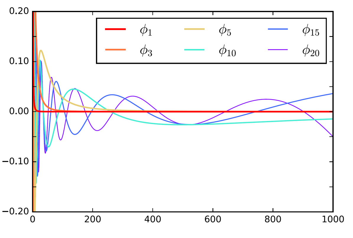
Figure 1: The filters obtained by the eigenvectors of $Z$.

The main advantage of spectral filtering is that for certain types of linear dynamical systems, in particular those with symmetric matrices $A$, the effective memory required to represent an observation at any point in the sequence in the spectral basis is independent of $\delta$!. This guarantee indicates that if we featurize the input into the spectral basis, we can potentially design models that are capable of efficiently and stably representing systems with extremely long memory. This striking fact motivates our derivation of the recurrent spectral architecture, and is the underlying justification for the performance and training stability gains we see in experiments.

1.1 Our Contributions

We start by proposing state space models with learned components that apply spectral filtering for their featurization. We consider two types of spectral filters, which augment the original spectral filters proposed in Hazan et al. (2017) with negative eigenvalues in two different ways.

Our main contribution is a neural architecture that is based on these spectral state space models. This neural architecture can be applied recursively in layers, resulting in an expressive architecture for modeling sequential data.

Finally we implement this neural architecture and apply it towards synthetically generated data as well as the Long Range Arena benchmark (Tay et al., 2021). We demonstrate that spectral state space models can stably and more efficiently learn on sequence modelling tasks with long range dependencies without the need for exponential parameterizations, particular initializations and normalizations.

Main Advantages of Spectral SSM.

Previous convolutional models for sequence modeling, surveyed in the related work section, learn the convolutions from the data. The filters used in Spectral SSM are theoretically-founded and fixed and thus parameter-free. In addition, our models are provably more expressive than Linear Dynamical Systems. The reason is that their expressiveness does not depend on the memory decay, nor on the dimension of the system, which are necessary in all other methods.

1.2 Related work

State space models.

SSMs for learning long range phenomenon have received much attention in the deep learning community in recent years. Gu et al. (2020) propose the HiPPO framework for continuous-time memorization, and shows that with a special class of system matrices $A$ (HiPPO matrices), SSMs have the capacity for long-range memory. Subsequently, Gu et al. (2021b) propose the Linear State-Space Layer (LSSL), where the system matrix is learnable. The LSSL can be viewed as a recurrence in the state domain and a convolution in the time domain, and generalizes particular RNN and CNN architectures. For efficient learning of the system matrices, authors propose learning within a class of structured matrices that contain the HiPPO dynamics, and have efficient convolution schemes. However, the proposed method is numerically unstable in practice as well as memory-intensive. As a result, Gu et al. (2021a) develop the S4 parameterization to address these bottlenecks. The S4 parameterization restricts the system matrices $A$ to be normal plus low-rank, allowing for stable diagonalization of the dynamics. Under this parameterization, authors design memory and computationally efficient methods that are also numerically stable.

The S4 model has been further streamlined in later works. Gupta et al. (2022) simplify the S4 parameterization to diagonal system matrices, and shows that the diagonal state-space model (DSS) is competitive with S4 on several benchmarks. Smith et al. (2023) propose the S5 architecture, which improves upon S4 in two directions: 1) instead of having independent SISO SSMs in the feature dimension, S5 has one MIMO DSS that produces vector-valued outputs; 2) S5 uses efficient parallel scans in place of convolutions, bypassing custom-designed algorithms for computing the convolutional filters.

Motivated by the similarities between SSMs and RNNs, Orvieto et al. (2023) investigate whether deep RNNs can recover the performance of deep SSMs, and provide an affirmative answer. The proposed RNN architecture is a deep model with stacked Linear Recurrent Unit (LRU) layers. Each LRU has linear recurrence specified by a complex diagonal matrix, learned with exponential parameterization and proper normalization techniques. The deep LRU architecture has comparable computational efficiency as SSMs and matches their performance on benchmarks that require long-term memory. However, the paper also shows that without the specific modifications on linear RNNS, namely the stable exponential parameterization, gamma normalization and ring initialization, LRU fails to learn on certain challenging long-context modeling tasks.

Spectral filtering.

The technique of spectral filtering for learning linear dynamical systems was put forth in Hazan et al. (2017). This work studies online prediction of the sequence of observations $y_{t}$, and the goal is to predict as well as the best symmetric LDS using past inputs and observations. Directly learning the dynamics is a non-convex optimization problem, and spectral filtering is developed as an improper learning technique with an efficient, polynomial-time algorithm and near-optimal regret guarantees. Different from regression-based methods that aim to identify the system dynamics, spectral filtering’s guarantee does not depend on the stability of the underlying system, and is the first method to obtain condition number-free regret guarantees for the MIMO setting. Extension to asymmetric dynamical systems was further studied in Hazan et al. (2018).

Convolutional Models for Sequence Modeling

Exploiting the connnection between Linear dynamical systems and convolutions (as highlighted by Gu et al. (2021a)) various convolutional models have been proposed for sequence modelling. Fu et al. (2023) employ direct learning of convolutional kernels directly to sequence modelling but find that they underperform SSMs. They find the non-smoothness of kernels to be the culprit and propose applying explicit smoothing and squashing operations to the kernels to match performance on the Long Range Arena benchmark. The proposed still contains significantly large number of parameters growing with the sequence length. Li et al. (2022) identifies two key characteristics of convolutions to be crucial for long range modelling, decay in filters and small number of parameters parameterizing the kernel. The achieve this via a specific form of the kernel derived by repeating and scaling the kernel in a dyadic fashion. Shi et al. (2023) propose a multiresolution kernel structure inspired from the wavelet transform and multiresolution analysis.

All these methods parameterize the kernels with specific structures and/or add further regularizations to emulate the convolution kernels implied by SSMs. In contrast our proposed kernels are fixed and thereby parameter-free and the number of parameters scale in the number of kernels and not the size of the kernel. Furthermore our kernels are provably more expressive than linear dynamical systems capable of directly capturing and improving the performance of SSMs without the need for specific initializations. Naturally our kernels (see Fig 1) by default satisfy both the smoothness and the decay condition identified (and explicitly enforced) by Li et al. (2022) and Fu et al. (2023).

2 Preliminaries

Online sequential prediction.

Online sequential prediction is a game between a predictor/learner and nature in which iteratively at every time $t\in[L]$, the learner is presented an input $u_{t}\in{\mathbb{R}}^{d_{\mathrm{in}}}$. The learner $A$ then produces a candidate output $\hat{y}_{t}=\hat{y}_{t}(A)$ , and nature reveals the $t^{th}$ element of a target sequence $y_{t}\in{\mathbb{R}}^{d_{\mathrm{out}}}$. The learner then suffers an instantaneous loss

$$\|y_{t}-\hat{y}_{t}\|^{2}.$$

The task of the learner is to minimize regret which is defined as follows

$$\mbox{Regret}=\sum_{t=1}^{L}\|y_{t}-\hat{y}_{t}\|^{2}-\min_{A\in{\mathcal{A}}}\sum_{t=1}^{L}\|y_{t}-\hat{y}_{t}(A)\|^{2},$$

where ${\mathcal{A}}$ is a benchmark set of learning algorithms.

Linear Dynamical Systems:

An example benchmark set of methods is that of linear dynamical systems. Recall that a linear dymamical system (LDS) has four matrix parameters, $A\in{\mathbb{R}}^{N\times N},B\in{\mathbb{R}}^{N\times d_{\mathrm{in}}},C\in{\mathbb{R}}^{d_{\mathrm{out}}\times N},D\in{\mathbb{R}}^{d_{\mathrm{out}}\times d_{\mathrm{in}}}$. The system evolves and generates outputs according to the following equations

$$x_{t} \triangleq Ax_{t-1}+Bu_{t}.$$

$$\hat{y}_{t} \triangleq Cx_{t}+Du_{t}$$ (1)

Thus, an example class of benchmark algorithms ${\mathcal{A}}$ are all predictors that generate $\hat{y}_{t}$ according to these rules, for a fixed set of matrices $A,B,C,D$.

Spectral Filtering:

Another important set of predictors is one which is inspired by spectral filtering. For any $L$ define the following Hankel matrix $Z\in{\mathbb{R}}^{L\times L}$ whose entries are given by

$$Z[i,j]\triangleq\frac{2}{(i+j)^{3}-(i+j)}$$

It can be shown that $Z$ is a real PSD matrix and therefore admits a real spectral decomposition and the (non-negative) eigenvalues can be easily ordered naturally by their value. Let $\{(\sigma_{j}\in{\mathbb{R}},\phi_{j}\in{\mathbb{R}}^{T})\}_{j=1}^{L}$ be the eigenvalue-eigenvector pairs of $Z$ ordered to satisfy $\sigma_{1}\geq\sigma_{2}\geq\ldots\geq\sigma_{d}$. We consider a fixed number $K$ of the above eigenvectors. Algorithms in the spectral filtering class generate $\hat{y}_{t}$ as follows. For each $k\in K$, we first featurize the input sequence by projecting the input sequence until time $t$ on $\phi_{k}$, leading to a sequence $U_{t,k}\in{\mathbb{R}}^{d_{\mathrm{in}}}$ defined as

$$U_{t,k}=\sum_{i=1}^{t}u_{t-i}\cdot\phi_{k}(i).$$

The spectral filtering class is further parameterized by matrices $M^{u}_{1}\in{\mathbb{R}}^{d_{\mathrm{out}}\times d_{\mathrm{in}}}$, $M^{u}_{2}\in{\mathbb{R}}^{d_{\mathrm{out}}\times d_{\mathrm{in}}}$ and a set of matrices $M^{\phi}_{1},...,M^{\phi}_{K}\in{\mathbb{R}}^{d_{\mathrm{out}}\times d_{\mathrm{in}}}$. The output at time $t$ is then given by

$$\hat{y}_{t}=y_{t-1}+M^{u}_{1}u_{t}+M^{u}_{2}u_{t-1}+\sum_{k=1}^{K}M^{\phi}_{k}U_{t,k}.$$ (2)

Note that given an input sequence $u_{1:L}$ for any $k$, the $d_{\mathrm{in}}\times T$ matrix $U_{1:L,k}$ can be efficiently computed via convolutions along the time dimension $L$ in total time $O(d_{\mathrm{in}}\cdot L\log(L))$. The following theorem (proved in Hazan et al. (2017)) establishes that the spectral filtering class of predictors approximately contains bounded linear dynamical systems with positive semi-definite $A$.

Theorem 2.1.

Given any $A,B,C,D$ such that $A$ is a PSD matrix with $\|A\|\leq 1$ and given any numbers $K\in\mathbb{I}^{+},a\in{\mathbb{R}}^{+}$, there exists matrices $M^{u}_{1},M^{u}_{2},M^{\phi}_{1},...,M^{\phi}_{K}$, such that for all $L$ and all sequences $u_{1:L}$ satisfying $\|u_{t}\|\leq a$ for all $t\in[L]$ the following holds. Let $y^{\mathrm{LDS}}_{1:L}$ be the sequence generated by execution of the LDS given by $A,B,C,D$ (via (2)) and $y^{\mathrm{SF}}_{1:L}$ be the sequence generated by Spectral Filtering (via (2)) using the matrices $M^{u}_{1},M^{u}_{2},M^{\phi}_{1},...,M^{\phi}_{K}$. Then for all $t\in[L]$, we have that

$$\|y^{\mathrm{LDS}}_{t}-y^{\mathrm{SF}}_{t}\|^{2}\leq c_{1}\cdot L^{2.5}\cdot(c_{2}^{-\log(L)/K})$$

where $c_{1}$ depends upon $A,B,C,D,a$ and $c_{2}$ is a universal constant.

In the next section we build upon this predictor class to create neural networks that are sequential predictors with a special structure.

3 Spectral Transform Unit(STU)

In this section we use the Spectral Filtering class to create a neural network layer which is a sequence to sequence map, i.e. given an input sequence $\{u_{1}\ldots u_{L}\}\in{\mathbb{R}}^{d_{\mathrm{in}}}$, it produces an output sequence $\{y_{1}\ldots y_{L}\}\in{\mathbb{R}}^{d_{\mathrm{out}}}$.

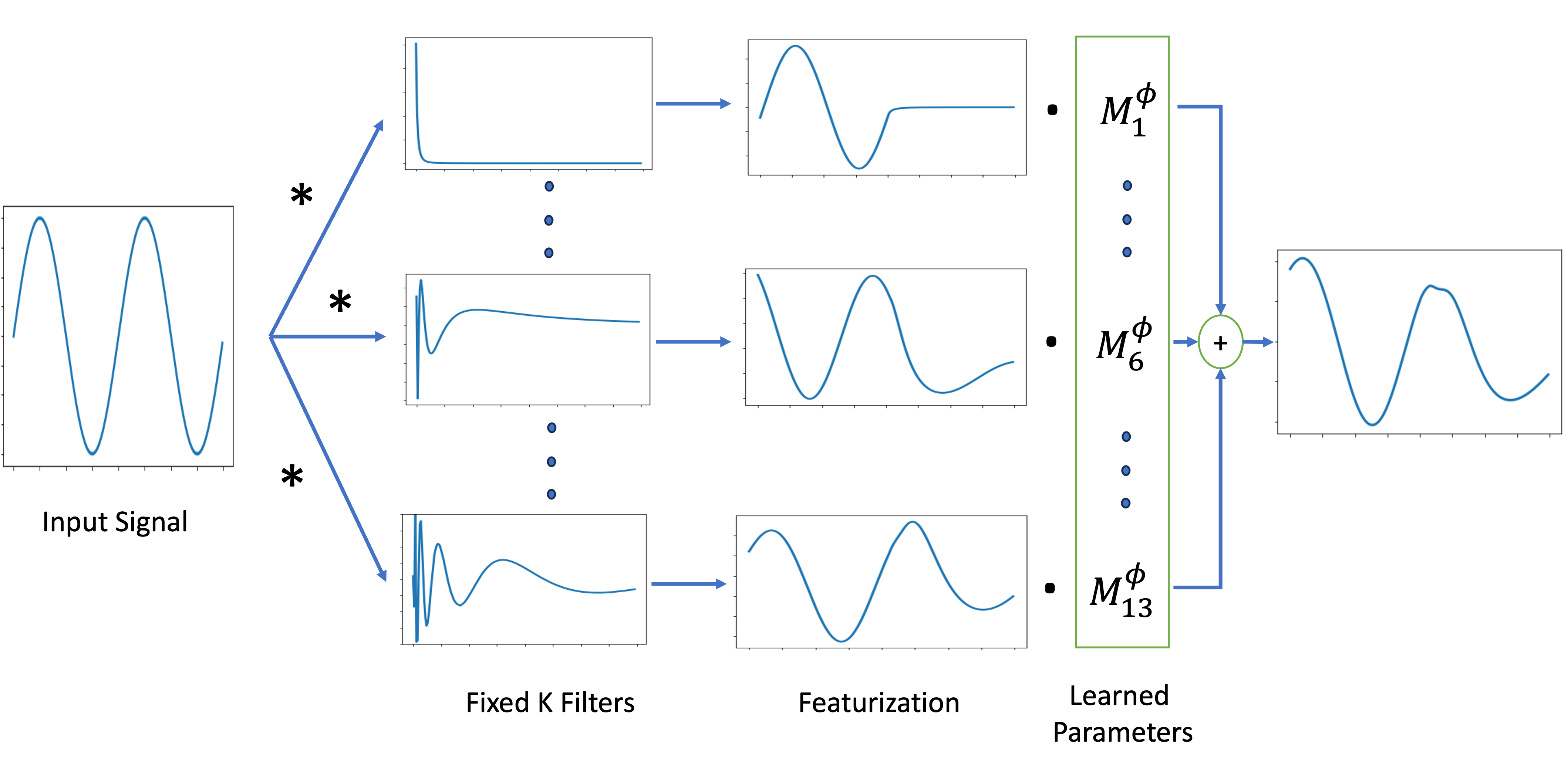
Figure 2: Schematic showing the spectral projection of the input sequence and how these features are used to produce the spectral component in the STU output (4). For simplicity we consider only the uni-dimensional input and output case but the operation is applied in parallel across every input dimension.

A single layer of STU (depicted in Figure 2) is parameterized by a number $K$, denoting the number of eigenfactors and matrices $M^{\phi+}_{1}\ldots M^{\phi+}_{K},M^{\phi-}_{1}\ldots M^{\phi-}_{K}\in{\mathbb{R}}^{d_{\mathrm{out}}\times d_{\mathrm{in}}},$ and $M^{u}_{1},M^{u}_{2},M^{u}_{3}\in{\mathbb{R}}^{d_{\mathrm{out}}\times d_{\mathrm{in}}}$. The matrices form the params of the layer. Further recall the Hankel matrix $Z\in{\mathbb{R}}^{L\times L}$ whose entries are given by

$$Z[i,j]\triangleq\frac{2}{(i+j)^{3}-(i+j)}.$$ (3)

and let $\{(\sigma_{j}\in{\mathbb{R}},\phi_{j}\in{\mathbb{R}}^{L})\}_{j=1}^{L}$ be the eigenvalue-eigenvector pairs of $Z$ ordered to satisfy $\sigma_{1}\geq\sigma_{2}\geq\ldots\sigma_{d}$.

Given an input sequence $\{u_{1}\ldots u_{L}\}\in{\mathbb{R}}^{d_{\mathrm{in}}}$, we first featurize the input sequence as follows. For any $t,k$, we begin by projecting the input sequence till time $t$ on fixed filters $\phi_{k}$, leading to two feature vectors $U^{+}_{t,k},U^{-}_{t,k}\in{\mathbb{R}}^{d_{\mathrm{in}}}$ defined as

$$U_{t,k}^{+}=\sum_{i=0}^{t-1}u_{t-i}\cdot\phi_{k}(i)\qquad U_{t,k}^{-}=\sum_{i=0}^{t-1}u_{t-i}\cdot(-1)^{i}\cdot\phi_{k}(i).$$

Note that for every $k$, the sequence of features $U_{1:L,k}$ can be computed efficiently via convolution. The output sequence $\{y_{1}\cdots y_{L}\}$ is then given by

$$\hat{y}_{t} =\underbrace{\vrule width=0.0pt,height=0.0pt,depth=13.77771pt\hat{y}_{t-2}+\sum_{i=1}^{3}M^{u}_{i}u_{t+1-i}}_{\mathrm{Auto-regressive\;Component}}+$$

$$\underbrace{\sum_{k=1}^{K}M^{\phi+}_{k}\sigma_{k}^{1/4}U^{+}_{t-2,k}+\sum_{k=1}^{K}M^{\phi-}_{k}\sigma_{k}^{1/4}U^{-}_{t-2,k}}_{\mathrm{Spectral\;Component}}.$$ (4)

The above output contains a small auto-regressive component that essentially allows for stable learning of the spectral component as the memory grows. The primary differences we observe from the original spectral filtering class (2) are the introduction of a negative part in the spectral component and the slight change in the auto-regressive component. Both of these changes are necessitated by the requirement to capture negative eigenvalues of $A$. Note that (4) corresponds to the specification of the algorithm presented in Hazan et al. (2018), when the eigenvalues are known to be real numbers. For completeness and ease of discourse we prove the following representation theorem in the Appendix which shows that the above class approximately contains any marginally-stable LDS with symmetric $A$.

Theorem 3.1.

Given any $A,B,C,D$ such that $A$ is a symmetric matrix with $\|A\|\leq 1$ and given any numbers $K\in\mathbb{I}^{+},a\in{\mathbb{R}}^{+}$, there exists matrices $M^{u}_{1},M^{u}_{2},M^{u}_{3},M^{\phi+}_{1}\ldots M^{\phi+}_{K},M^{\phi-}_{1}\ldots M^{\phi-}_{K}\in{\mathbb{R}}^{d_{\mathrm{out}}\times d_{\mathrm{in}}}$, such that for all $L$ and all sequences $u_{1:L}$ satisfying $\|u_{t}\|\leq a$ for all $t\in[L]$ the following holds. Let $y^{\mathrm{LDS}}_{1:L}$ be the sequence generated by execution of the LDS given by $A,B,C,D$ (via (2)) and $y^{\mathrm{SF}}_{1:L}$ be the sequence generated by Spectral Filtering (via (4)) using the matrices $M^{u}_{1},M^{u}_{2},M^{u}_{3},M^{\phi+}_{1}\ldots M^{\phi+}_{K},M^{\phi-}_{1}\ldots M^{\phi-}_{K}$. Then for all $t\in[T]$, we have that

$$\|y^{\mathrm{LDS}}_{t}-y^{\mathrm{SF}}_{t}\|^{2}\leq c_{1}\cdot L^{3.5}\cdot c_{2}^{-\log(L)/K}$$

where $c_{1}$ depends upon $A,B,C,D,a$ and $c_{2}$ is a universal constant.

The proof of the above theorem is provided in the appendix along with an alternative version of spectral filtering using slightly modified filters which also provide the same guarantee.

Remark 3.2.

Comparing Theorem 3.1 (our contribution) and Theorem 2.1 (Theorem 1 from (Hazan et al., 2017)), we note the following differences. Firstly the theorem holds for symmetric matrices and not just PSD matrices. In the paper (Hazan et al., 2017), the authors allude to a direct extension for the symmetric case but we believe that extension is not fully correct. We use a similar idea to prove this theorem. Secondly a minor difference is that in the sequential prediction setting the prediction is auto-regressive, i.e. uses its own $y$ to make the future predictions.

Computational complexity

- As noted before the features $U^{+}$ and $U^{-}$ can be computed efficiently in total time $O(k\cdot L\cdot d_{\mathrm{in}}\log(L))$. Further computation of the spectral component takes $O(K\cdot L\cdot d_{\mathrm{in}}\cdot d_{\mathrm{out}})$ and the autoregressive part can be implemented in total time $O(L\cdot d_{\mathrm{in}}\cdot d_{\mathrm{out}})$. Therefore the overall runtime is $O(k\cdot L\cdot d_{\mathrm{in}}\cdot(\log(L)+d_{\mathrm{out}}))$.

3.1 Experiment: Learning a marginally-stable LDS

We provide a simple synthetic evaluation of the stability and training efficiency afforded by the STU. We consider a low-dimensional linear system $A,B,C,D$ generated as follows. $B\in{\mathbb{R}}^{4\times 3},C\in{\mathbb{R}}^{3\times 4}$ are matrices with iid unit Gaussian entries. $D$ is a diagonal matrix with iid unit Gaussian entries and $A$ is a diagonal matrix with $A_{ii}\sim 0.9999*Z$ where $Z$ is a random sign. By design this is a system with a very high stability constant ($\sim 10^{4}$). As a training dataset we generated $\{(u_{i},y_{i})\}$ where $u_{i}$ is a random input sequence and $y_{i}$ is the output generated by applying the linear dynamical system on $u_{i}$. We perform mini-batch (batch size 1) training with the l2 loss. As comparison we perform the same procedure with an LRU (Linear Recurrent Unit) layer as proposed by Orvieto et al. (2023) which directly parameterizes the linear system. The results of the training loss as seen by the two systems are presented in Figure 3.

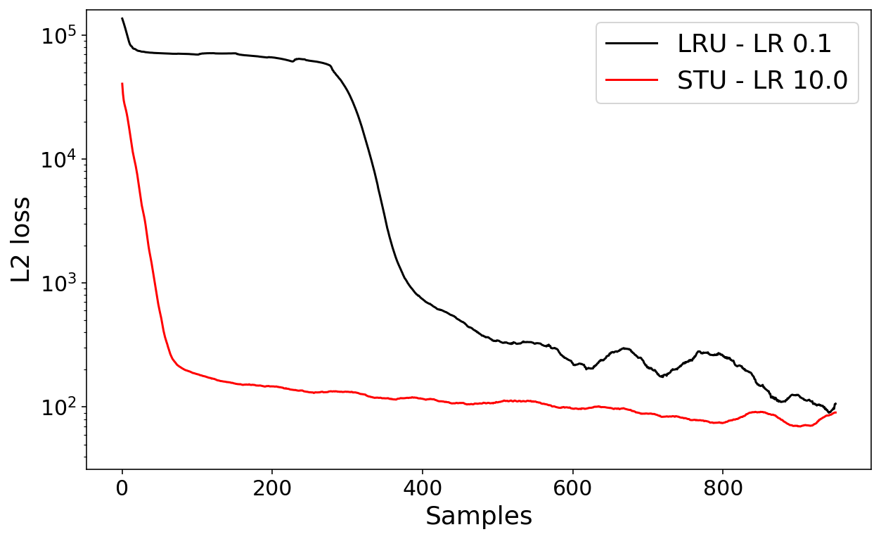
Figure 3: Dynamics for learning a marginally stable LDS: (Smoothed) Learning curves for single STU (red) vs single LRU layer (black). Learning rate was tuned for both models.

We use all the initialization/normalization techniques as recommended by Orvieto et al. (2023) for LRU including the stable exponential parameterization, $\gamma$-normalization and ring-initialization. Indeed we find that all these tricks were necessary to learn this system at all. We provide more details about the ablations and other hyperparameter setups in the appendix. We observe that the STU is significantly more efficient at learning the LDS as opposed to the LRU. We further find that there is a wide range of LRs where the STU has a stable optimization trajectory and the loss decreases continuously highlighting the advantages of a convex parameterization. On the other hand, LRU is able to eventually learn the system at the right learning rates, it requires almost 8x the number of samples to get to a system with non-trivial accuracy. More details can be found in the appendix. Curiously we observe that for the LRU training plateaus completely for the first 50% of training highlighting the difficulty of optimization via a non-convex landscape.

The STU layer in the previous experiment employs $K=25$. In Figure 4 we plot the performance of STU at various levels of $K$. As predicted by the theory we observe an exponential decay in the error as $K$ increases with the error effectively plateauing after $K\geq 15$.

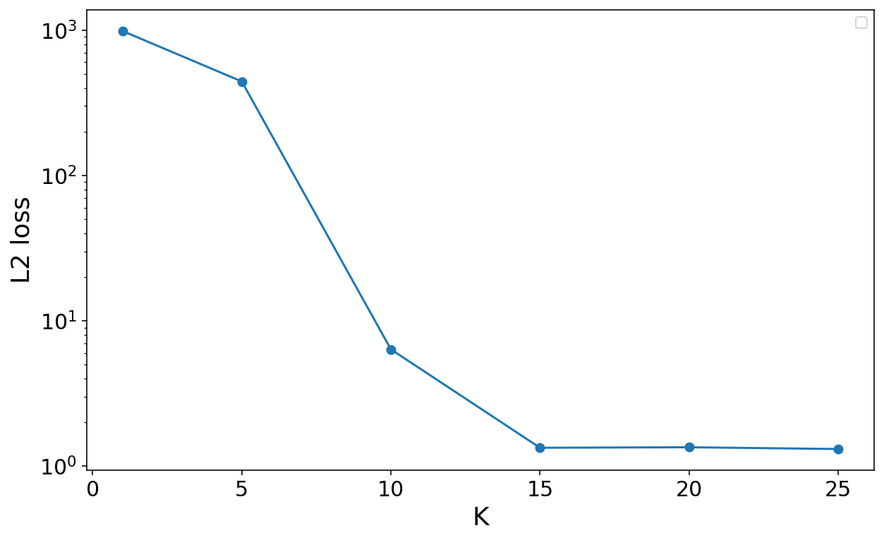
Figure 4: Error obtained by an STU layer as a function of the model parameter K. We observe an exponential drop in the reconstruction loss as predicted by the analysis.

4 Stacked STU

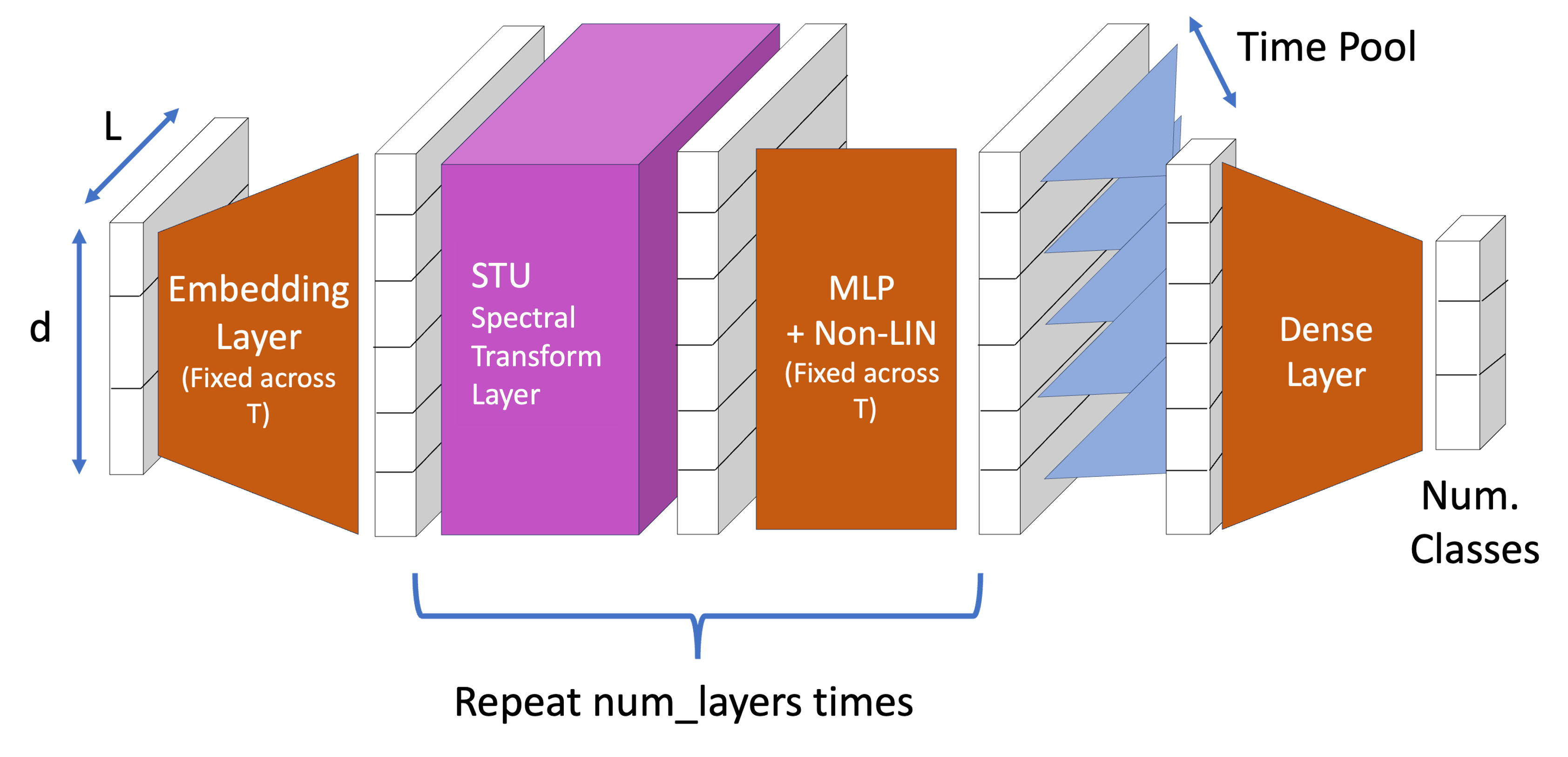
Figure 5: Schematic displaying a multi-layer STU model. Following the approach in the SSM literature non-linearities have been separated from the sequence to sequence transform to allow for efficient training and inference.

To increase the representation capacity and to maintain the efficiency of prediction through linear dynamical systems, proposed models in the SSM literature take the form of stacking these sequence to sequence transforms into multiple layers. Non-linearities in the model can then be introduced by sandwiching them as layers lying in between these sequence to sequence transforms.

In this paper we closely follow the stacking approach followed by Orvieto et al. (2023), replacing the LRU layers appropriately by STU layers. A schematic for the resultant multi-layer model is displayed in Figure 5. In a nutshell, the input sequence is first embedded via a time-invariant embedding function followed by multiple repetitions of alternating STU layers and non-linearities (in particular we use GLU). Finally the resulting output is time-pooled followed by a final readout layer according to the task at hand. This composite model can now be trained in a standard fashion via back-propagation and other commonly used deep-learning optimization techniques.

4.1 Experiments on Long Range Arena (Tay et al., 2021)

We evaluate the stacked STU model on the Long Range Arena (LRA) benchmark (Tay et al., 2021). This benchmark aims to assess the performance of sequence prediction models in long-context scenarios and consists of six tasks of various modalities, including text and images. The context length for the tasks ranges from 1K to 16K, and the tasks require capabilities such as hierarchical reasoning, matching and retrieval, and visual-spatial understanding. SSMs (Gu et al., 2021a) have shown significantly superior performance on most of the tasks compared to Transformer architectures. In particular for the hardest task in the suite, PathX (image classification with a context length of 16K), no transformer model has been able to achieve anything beyond the accuracy of random guessing. We provide the evaluation of the stacked STU model on the two hardest tasks namely PathFinder and PathX in the table below.

We compare our performance against the ablation carried out by Orvieto et al. (2023) who find that ring initialization, stable exponential parameterization and $\gamma$-normalization are all crucial towards learning these tasks. In particular as reported by Orvieto et al. (2023) all three of the above interventions were necessary to learn on PathX to any non-trivial accuracy. This is a result of the much larger context length of 16K employed by the PathX task. On the other hand we find that the the stacked STU (with the STU component exactly as represented by (4)) is sufficient to learn on both these tasks to relatively high accuracies. Notably we do not require any other normalizations or initialization techniques (we randomly initialize our M matrices using standard Glorot initialization). This result in particular confirms and highlights the theoretical stability afforded by the STU even under learning tasks involving large sequence lengths.

Model	Specification	Pathfinder	PathX
STU	Eqn (4) (K=16)	91.23	87.2
LRU	Complex Dense A	✗	✗
	$\Lambda$ Exp. Param.	65.4	✗
	$\Lambda$ Stable Exp. Param.	93.5	✗
	+ Ring Init.	94.4	✗
	+ $\gamma$-Norm.	95.1	94.2

Table 1: Comparison of the basic stacked STU model against LRU ablations in Orvieto et al. (2023)

In the next section we highlight a simple technique towards significantly improving the achieved accuracy for the stacked STU model.

5 Hybrid Temporal and Spectral Units

	CIFAR	ListOps	Text	Retrieval	Pathfinder	PathX
S4	91.1	59.6	86.8	90.9	94.2	96.4
S4D - LEGS	89.9	60.5	86.2	89.5	93.1	91.9
S5	90.1	62.2	89.3	91.4	95.3	98.6
LRU	89	60.2	89.4	89.9	95.1	94.2
AR-STU	91.3	60.33	89.6	90.0	95.6	90.1

Table 2: Comparison of the STU model against various proposed SSM models on the LRA benchmark: Bold values indicate the best for that task. We find that STU is competitive across all the workloads without the need for carefully designed initializations, discretizations or normalizations. We report the median over 5 trials for our experiments.

A simple extension to the STU model (Equation (4)) is to parameterize the dependence of $y_{t}$ on $y_{t-2}$ with a parameter $M_{y}$, leading to the following prediction model

$$\hat{y}_{t} =\underbrace{\vrule width=0.0pt,height=0.0pt,depth=13.77771pt\boldsymbol{M^{y}}\hat{y}_{t-2}+\sum_{i=1}^{3}M^{u}_{i}u_{t+1-i}}_{\mathrm{Auto-regressive\;Component}}+$$

$$\underbrace{\sum_{k=1}^{K}M^{\phi+}_{k}\sigma_{k}^{1/4}U^{+}_{t-2,k}+\sum_{k=1}^{K}M^{\phi-}_{k}\sigma_{k}^{1/4}U^{-}_{t-2,k}}_{\mathrm{Spectral\;Component}}.$$ (5)

Setting $M^{y}=I$ we recover the guarantees afforded by Theorem 3.1 and thus the above model is strictly more powerful. We find that the above change leads to significant improvements over the accuracy achieved by the simple STU model. We can further extend the auto-regression to depend on multiple previous $y$ as opposed to just $y_{t-2}$. Indeed as the following theorem shows adding sufficiently long auto-regression is powerful enough to capture any LDS.

Theorem 5.1.

Given an LDS parameterized by $A\in{\mathbb{R}}^{d\times d},B,C,D$, there exist coefficients $\alpha_{1:d}$ and matrices $\Gamma_{0:d}$ such that given any input sequence $u_{1:L}$, the output sequence $y_{1:L}$ generated by the action of the LDS on the input satisfies for all $t$

$$y_{t}=\sum_{i=1}^{d}\alpha_{i}y_{t-i}+\sum_{i=0}^{d}\Gamma_{i}u_{t-i}$$

This is a well-known observation and we provide a proof in the appendix (Section D). Motivated by the above theorem we modify the definition of AR-STU to add auto-regression over the previously produced outputs. In particular given a parameter $k_{y}$ we define AR-STU the model as

$$\hat{y}_{t} =\underbrace{\vrule width=0.0pt,height=0.0pt,depth=13.77771pt\sum_{i=1}^{k_{y}}\boldsymbol{M^{y}_{i}}\hat{y}_{t-i}+\sum_{i=1}^{3}M^{u}_{i}u_{t+1-i}}_{\mathrm{Auto-regressive\;Component}}+$$

$$\underbrace{\sum_{k=1}^{K}M^{\phi+}_{k}\sigma_{k}^{1/4}U^{+}_{t-2,k}+\sum_{k=1}^{K}M^{\phi-}_{k}\sigma_{k}^{1/4}U^{-}_{t-2,k}}_{\mathrm{Spectral\;Component}}.$$ (6)

In Table 2, we evaluate the performance of AR-STU. For most tasks including including ListOps, Text, Retrieval and PathX we find that setting $k_{y}=2$ is sufficient to get optimal results. For two tasks, CIFAR and Pathfinder, we found that $k_{y}=32$ led to significant performance gains. We initialize the $M^{y}_{i}$ parameters to be such that they recover the STU model at initialization, i.e. we set $M^{y}_{2}=\alpha\cdot I$ and $M^{y}_{i}=0$ for all $i\neq 2$ at initialization (where $\alpha$ is a hyper-parameter, but we find the choice of $\alpha=0.9$ to be uniformly optimal). Overall we find that the STU model is competitive with state space models across the entire variety of tasks in the Long Range Arena without the need for specific initializations, discretizations and normalizations. We provide details of our experimental setup and more results in the appendix.

6 Conclusion

Insprired by the success of State Space Models, we present a new theoretically-founded deep neural network architecture, Spectral SSM, for sequence modelling based on the Spectral Filtering algorithm for learning Linear Dynamical Systems. The SSM performs a reparameterization of the LDS and is guaranteed to learn even marginally stable symmetric LDS stably and efficiently. We demonstrate the core advantages of the Spectal SSM, viz. robustness to long memory through experiments on a synthetic LDS and the Long Range Arena benchmark. We find that the Spectral SSM is able to learn even in the presence of large context lengths/memory without the need for designing specific initializations, discretizations or normalizations which were necessary for existing SSMs to learn in such settings.

Impact statement

This paper presents work whose goal is to advance the field of Machine Learning. There are many potential societal consequences of our work, none which we feel must be specifically highlighted here.

Appendix A Proof of Theorem 3.1

We begin by observing that without loss of generality we can assume that $A$ is a real-diagonal matrix. This can be ensured by performing a spectral decomposition of $A=U\Sigma U^{\top}$ and absorbing the $U,U^{\top}$ by redefining the system. Before continuing with the proof, we will provide some requisite definitions and lemmas. Define the following vector for any $\alpha\in{\mathbb{R}}$, $\mu(\alpha)\in{\mathbb{R}}^{L}$, with $\mu(\alpha)(i)=(\alpha-1)\alpha^{i-1}$. Further define the Hankel matrix $H$ as

$$Z\triangleq\int_{0}^{1}\mu(\alpha)\mu(\alpha)^{\top}d\alpha.$$

As the following lemma shows the Hankel matrix $Z$ above is the same Hankel matrix defined in the definition of STU (3).

Lemma A.1.

$Z$ is a Hankel matrix with entries given as

$$Z(i,j)=\frac{2}{(i+j)^{3}-(i+j)}$$

Lemma A.2.

We have that the following statements hold regarding $\mu(\alpha)$ for any $\alpha\in[0,1]$,

• $|\mu(\alpha)|^{2}\leq 1$

• For any $\alpha\in[0,1]$ and any unit vector $v$ we have that

  $$(\mu(\alpha)^{\top}v)^{2}\leq 12(v^{\top}Hv)$$

Lemma A.3.

For any $\alpha\in[0,1]$, let $\tilde{\mu}(\alpha)$ be the projection of $\mu(\alpha)$ on the subspace spanned by top $k$ eigenvectors of $Z$, then we have that

$$\|\mu(\alpha)-\tilde{\mu}(\alpha)\|^{2}\leq 12\sum_{i=k+1}^{L}\sigma_{i}$$

Finally the following lemma from (Hazan et al., 2017) shows that the spectrum of the matrix $Z$ decays exponentially.

Lemma A.4 (Lemma E.3 (Hazan et al., 2017)).

Let $\sigma_{j}$ be the top $j^{th}$ eigenvalue of $Z$. Then we have that

$$\sigma_{j}\leq\min\left(3/4,\Gamma c^{-j/\log(L)}\right)$$

where $c=e^{\pi^{2}/4}$ and $\Gamma\leq 10^{-6}$ is an absolute constant.

We now move towards proving Theorem 3.1. Consider the following calculation for the LDS sequence $y_{t}^{\mathrm{LDS}}$

$$y_{t}^{\mathrm{LDS}}=\sum_{i=0}^{T}CA^{i}Bu_{t-i}+Du_{t},$$

and therefore we have that

$$y_{t}^{\mathrm{LDS}}-y_{t-2}^{\mathrm{LDS}}=(CB+D)u_{t}+CABu_{t-1}-Du_{t-2}+\underbrace{\sum_{i=0}^{T}C(A^{i+2}-A^{i})Bu_{t-2-i}}_{\mathrm{Term\;of\;Interest}}$$

For any $t_{1}\geq t_{2}$ we define the matrix $\bar{U}_{\{t_{1}:t_{2}\}}\in{\mathbb{R}}^{d_{\mathrm{out}}\times t_{1}-t_{2}+1}$ whose $i^{th}$ column is the input vector $u_{t_{1}-i+1}$. We allow $t_{2}$ to be negative and by convention assume $u_{t}=0$ for any $t\leq 0$. Denote the diagonal entries of $A$ by $\{\alpha_{l}\}_{l=1}^{d_{h}}$, i.e. $\alpha_{l}=A(l,l)$. The term of interest above can then be written as

$$\sum_{i=0}^{L}C(A^{i+2}-A^{i})Bu_{t-2-i}$$

$$=\sum_{l=1}^{d_{h}}(c_{l}\otimes b_{l})\left(\sum_{i=0}^{L}(\alpha_{l}^{i+2}-\alpha_{l}^{i})u_{t-2-i}\right)$$

$$=\sum_{l:\alpha_{l}\geq 0}(c_{l}\otimes b_{l})\left(\sum_{i=0}^{L}(\alpha_{l}^{2}-1)\alpha_{l}^{i}u_{t-2-i}\right)+\sum_{l:\alpha_{l}<0}(c_{l}\otimes b_{l})\left(\sum_{i=0}^{L}(\alpha_{l}^{2}-1)\alpha_{l}^{i}u_{t-2-i}\right)$$

$$=\sum_{l:\alpha_{l}\geq 0}(\alpha_{l}+1)(c_{l}\otimes b_{l})\left(\sum_{i=0}^{L}(\alpha_{l}-1)\alpha_{l}^{i}u_{t-2-i}\right)+\sum_{l:\alpha_{l}<0}(1+|\alpha_{l}|)(c_{l}\otimes b_{l})\left(\sum_{i=0}^{L}(|\alpha_{l}|-1)|\alpha_{l}|^{i}(-1)^{i}u_{t-2-i}\right)$$

$$=\sum_{l:\alpha_{l}\geq 0}(\alpha_{l}+1)(c_{l}\otimes b_{l})\left(\bar{U}_{\{t-2:t-1-L\}}\mu(\alpha)\right)+\sum_{l:\alpha_{l}<0}(|\alpha_{l}|+1)(c_{l}\otimes b_{l})\left(\bar{U}_{\{t-2:t-1-L\}}\odot\mathbf{1}^{\pm}\right)\mu(|\alpha_{l}|)$$

where $\mathbf{1}^{\pm}\in{\mathbb{R}}^{d_{\mathrm{out}}\times L}$ is defined as the matrix whose every row is the alternating sign vector $[1,-1,1,-1\ldots]$) and $\odot$ is Hadamard product (i.e. entry-wise multiplication).

$$y_{t}^{\mathrm{LDS}}-y_{t-2}^{\mathrm{LDS}} =(CB+D)u_{t}+CABu_{t-1}-Du_{t-2}+\underbrace{\sum_{l:\alpha_{l}\geq 0}(\alpha_{l}+1)(c_{l}\otimes b_{l})\left(\bar{U}_{\{t-2:t-1-L\}}\mu(\alpha)\right)}_{PositivePart}$$

$$+\underbrace{\sum_{l:\alpha_{l}<0}(|\alpha_{l}|+1)(c_{l}\otimes b_{l})\left(\bar{U}_{\{t-2:t-1-L\}}\odot\mathbf{1}^{\pm}\right)\mu(|\alpha_{l}|)}_{NegativePart}$$

Recall that we defined the sequence $\{\sigma_{k},\phi_{k}\}_{k=1}^{L}$ to be the eigenvalue and eigenvector pairs for the Hankel matrix $Z$. For any $\alpha$ we define the projection of $\mu(\alpha)$ on the top $k$ eigenvectors as $\tilde{\mu}(\alpha)$, i.e. $\tilde{\mu}(\alpha)=\sum_{k=1}^{K}(\mu(\alpha_{l})^{\top}\phi_{k})\phi_{k}$. Further define STU parameters as follows

$$M_{1}^{u}=CB+D,M_{2}^{u}=CAB,M_{3}^{u}=-D$$

$$M_{k}^{\phi+}=\sum_{l:\alpha_{l}\geq 0}(\alpha_{l}+1)(\mu(\alpha_{l})^{\top}\phi_{k})\sigma_{k}^{-1/4}(c_{l}\otimes b_{l})$$

$$M_{k}^{\phi-}=\sum_{l:\alpha_{l}<0}(|\alpha_{l}|+1)(\mu(|\alpha_{l}|)^{\top}\phi_{k})\sigma_{k}^{-1/4}(c_{l}\otimes b_{l})$$

The definition of STU prediction (4), using the above parameters, implies that the predicted sequence satisfies

$$y_{t}^{\mathrm{STU}}-y_{t-2}^{\mathrm{STU}}=(CB+D)u_{t}+CABu_{t-1}-Du_{t-2} +\sum_{l:\alpha_{l}\geq 0}(\alpha_{l}+1)(c_{l}\otimes b_{l})\left(\bar{U}_{\{t-2:t-1-L\}}\right)\left(\underbrace{\sum_{k=1}^{K}(\mu(\alpha_{l})^{\top}\phi_{k})\phi_{k}}_{=\tilde{\mu}(\alpha)}\right)$$

$$+\sum_{l:\alpha_{l}<0}(|\alpha_{l}|+1)(c_{l}\otimes b_{l})\left(\bar{U}_{\{t-2:t-1-L\}}\odot\mathbf{1}^{\pm}\right)\left(\underbrace{\sum_{k=1}^{K}(\mu(|\alpha_{l}|)^{\top}\phi_{k})\phi_{k}}_{=\tilde{\mu}(|\alpha_{l}|)}\right)$$

Combining the above displays we get that

$$y_{t}^{\mathrm{LDS}}-y_{t}^{\mathrm{STU}}=y_{t-2}^{\mathrm{LDS}}-y_{t-2}^{\mathrm{STU}} +\sum_{l:\alpha_{l}\geq 0}(\alpha_{l}+1)(c_{l}\otimes b_{l})\left(\bar{U}_{\{t-2:t-1-L\}}\right)\left(\mu(\alpha)-\tilde{\mu}(\alpha)\right)$$

$$+\sum_{l:\alpha_{l}<0}(|\alpha_{l}|+1)(c_{l}\otimes b_{l})\left(\bar{U}_{\{t-2:t-1-L\}}\odot\mathbf{1}^{\pm}\right)\left(\mu(|\alpha_{l}|)-\tilde{\mu}(|\alpha_{l}|)\right)$$

Using triangle inequality, the fact that the input and the system are bounded and Lemma A.3 we get that there exists a universal constant $c$ such that

$$\|y_{t}^{\mathrm{LDS}}-y_{t}^{\mathrm{STU}}\|\leq\|y_{t-2}^{\mathrm{LDS}}-y_{t-2}^{\mathrm{STU}}\|+c\cdot L^{2}\sqrt{\sum_{i=K+1}^{L}\sigma_{i}}$$

Applying the above equation recursively and Lemma A.4 we get that there exists a universal constant $c$ such that

$$\|y_{t}^{\mathrm{LDS}}-y_{t}^{\mathrm{STU}}\|\leq O\left(L^{3}\sqrt{\sum_{i=K+1}^{L}\sigma_{i}}\right)\leq O\left(L^{3.5}\cdot c^{-K/\log(L)}\right),$$

which finishes the proof of the theorem.

A.1 Proofs of Lemmas

Proof of Lemma A.1.

The lemma follows from the following simple calculations.

$$Z(i,j)=\int_{0}^{1}(\alpha-1)^{2}\alpha^{i+j-2}d\alpha=\int_{0}^{1}\left(\alpha^{i+j}+\alpha^{i+j-2}-2\alpha^{i+j-1}\right)d\alpha =\frac{1}{(i+j+1)}+\frac{1}{(i+j-1)}-\frac{2}{(i+j)}$$

$$=\frac{2}{(i+j)^{3}-(i+j)}$$

∎

Lemma A.3 is immediate from the second part of Lemma A.2. We show Lemma A.2 below.

Proof of Lemma A.2.

By definition $\mu(\alpha)=0$ for $\alpha\in\{0,1\}$. Otherwise we have that for all $\alpha\in(0,1)$,

$$|\mu(\alpha)|^{2}=\sum_{i=1}^{T}(\alpha-1)^{2}\alpha^{2i-2}\leq\frac{(\alpha-1)^{2}}{(1-\alpha^{2})}\leq\frac{1-\alpha}{1+\alpha}\leq 1-\alpha$$

To prove the second part we consider drawing $\alpha$ from the uniform distribution between $[0,1]$. We get that

$$E[(\mu(\alpha)^{\top}v)^{2}]=v^{\top}Zv$$

We now show that the worst case value is not significantly larger than the expectation. To this end we consider the function $f(\alpha)=(\mu(\alpha)^{\top}v)^{2}$ and we show that this is a 6-Lipschitz function. To this end consider the following,

$$\left\|\frac{\partial\mu(\alpha)}{\partial\alpha}\right\|_{2}^{2} =\sum_{i=0}^{T-1}\left\{\left|\frac{\partial}{\partial{\alpha}}(1-\alpha)\alpha^{i}\right|^{2}\right\}$$

$$=\sum_{i=0}^{T-1}\left((1-\alpha)i\alpha^{i-1}-\alpha^{i}\right)^{2}$$

$$\leq 2(1-\alpha)^{2}\sum_{i=1}^{T-1}i^{2}\alpha^{2(i-1)}+2\sum_{i=0}^{T-1}\alpha^{2i} (a+b)^{2}\leq 2(a^{2}+b^{2})$$

$$\leq 2(1-\alpha)^{2}\left(\frac{1}{(1-\alpha^{2})^{2}}+\frac{2\alpha^{2}}{(1-\alpha^{2})^{3}}\right)+\frac{2}{1-\alpha^{2}} \sum_{i=1}^{\infty}i^{2}\beta^{i-1}=\frac{1}{(1-\beta)^{2}}+\frac{2\beta}{(1-\beta)^{3}}$$

$$=\frac{2}{(1+\alpha)^{2}}+\frac{4\alpha^{2}}{(1-\alpha^{2})(1+\alpha)^{2}}+\frac{2}{1-\alpha^{2}}.$$

Therefore we have that for all $\alpha\in[0,1]$,

$$\frac{\partial f(\alpha)}{\partial\alpha} =2(\mu(\alpha)^{\top}v)\left(\frac{\partial\mu(\alpha)^{\top}}{\partial\alpha}v\right)\leq 2\|\mu(\alpha)\|\|v\|^{2}\|\frac{\partial\mu(\alpha)}{\partial\alpha}\|$$

$$\leq 2\sqrt{(1-\alpha)*\left(\frac{2}{(1+\alpha)^{2}}+\frac{4\alpha^{2}}{(1-\alpha^{2})(1+\alpha)^{2}}+\frac{2}{1-\alpha^{2}}\right)}$$

$$\leq 2\sqrt{\left(\frac{2(1-\alpha)}{(1+\alpha)^{2}}+\frac{4\alpha^{2}}{(1+\alpha)^{3}}+\frac{2}{1+\alpha}\right)}\leq 6.$$

Now for the positive function $f(\alpha)$ which is $6$-Lipschitz on $[0,1]$ let the maximum value be $R$. It can be seen the lowest expected value of $f(\alpha)$ over the uniform distribution over $[0,1]$, one can achieve is $R^{2}/2*6$ and therefore we have that

$$R^{2}/12\leq v^{\top}Zv\Rightarrow R\leq\sqrt{12v^{\top}Hv},$$

which finishes the proof.

∎

Appendix B Alternative Representation for capturing negative eigenvalues

In this section we setup an alternative version of STU wherein a different Hankel matrix is used but one can get a similar result. As before a single layer of STU (depicted in figure 2) is parameterized by a number $K$, denoting the number of eigenfactors and matrices $M^{\phi}_{1}\ldots M^{\phi}_{K}\in{\mathbb{R}}^{d_{\mathrm{out}}\times d_{\mathrm{in}}},$ and $M^{u}_{1},M^{u}_{2},M^{u}_{3}\in{\mathbb{R}}^{d_{\mathrm{out}}\times d_{\mathrm{in}}}$. The matrices form the params of the layer. We use a different Hankel matrix $Z_{L}\in{\mathbb{R}}^{L\times L}$ whose entries are given by

$$Z_{L}[i,j]\triangleq((-1)^{i+j-2}+1)\cdot\frac{8}{(i+j+3)(i+j-1)(i+j+1)}.$$ (7)

and let $\{(\sigma_{j}\in{\mathbb{R}},\phi_{j}\in{\mathbb{R}}^{T})\}_{j=1}^{T}$ be the eigenvalue-eigenvector pairs of $Z_{L}$ ordered to satisfy $\sigma_{1}\geq\sigma_{2}\ldots\sigma_{d}$.

Given an input sequence $\{u_{1}\ldots u_{L}\}\in{\mathbb{R}}^{d_{\mathrm{in}}}$, as before we first featurize the input sequence by projecting the input sequence till time $t$ on fixed filters $\phi_{k}$. The main difference is that we do not need to create a negative featurization now. We define

$$X_{t,k}=\sum_{i=0}^{t-1}u_{t-i}\cdot\phi_{k}(i).$$

Note that for every $k$, the sequence of features $X_{1:T,k}$ can be computed efficiently via convolution. The output sequence $\{y_{1}\cdots y_{T}\}$ is then given by

$$\hat{y}_{t}=\underbrace{\vrule width=0.0pt,height=0.0pt,depth=13.77771pt\hat{y}_{t-2}+\sum_{i=1}^{3}M^{u}_{i}u_{t+1-i}}_{\mathrm{Auto-regressive\;Component}}+\underbrace{\sum_{k=1}^{K}M^{\phi}_{k}\sigma_{k}^{1/4}X_{t-2,k}}_{\mathrm{Spectral\;Component}}.$$ (8)

We prove the following representation theorem which shows that the above class approximately contains any marginally-stable LDS with symmetric $A$.

Theorem B.1.

Given a bounded input sequence $u_{1:L}$ and given any bounded matrices $A,B,C,D$ with $A$ being a symmetric matrix let $y^{\mathrm{LDS}}_{1:L}$ be the sequence generated by execution of the LDS given by $A,B,C,D$ (via (2)). There exists matrices $M^{u}_{1},M^{u}_{2},M^{u}_{3},M^{\phi}_{1}\ldots M^{\phi}_{K}\in{\mathbb{R}}^{d_{\mathrm{out}}\times d_{\mathrm{in}}}$ such that the outputs $y^{\mathrm{SF}}_{1:T}$ generated by Spectral Filtering (via (4)) satisfies for all $t\in[L]$,

$$\|y^{\mathrm{LDS}}_{t}-y^{\mathrm{SF}}_{t}\|^{2}\leq O(L^{3.5}\cdot c^{-K/\log(L)})$$

where c is a universal constant.

In the following we prove the above theorem.

B.1 Proof of Theorem B.1

Without loss of generality we assume that $A$ is a real-diagonal matrix. Before continuing with the proof, we will provide some requisite definitions and lemmas. Define the following vector for any $\alpha$, $\mu(\alpha)\in{\mathbb{R}}^{T}$, with $\mu(\alpha)(i)=(\alpha^{2}-1)\alpha^{i-1}$. Further define the Hankel matrix $H$ as

$$Z\triangleq\int_{-1}^{1}\mu(\alpha)\mu(\alpha)^{\top}d\alpha$$

As the following lemma shows the Hankel matrix $Z$ above is the same Hankel matrix $Z_{L}$ defined in the definition of STU (7).

Lemma B.2.

$Z$ is a Hankel matrix with entries given as

$$Z(i,j)=((-1)^{i+j-2}+1)\cdot\frac{8}{(i+j+3)(i+j-1)(i+j+1)}$$

Proof.

Consider the following simple computations

$$H(i,j) =\int_{-1}^{1}(\alpha^{2}-1)^{2}\alpha^{i+j-2}d\alpha$$

$$=\int_{-1}^{0}(\alpha^{2}-1)^{2}\alpha^{i+j-2}d\alpha+\int_{0}^{1}(\alpha^{2}-1)^{2}\alpha^{i+j-2}d\alpha$$

$$=\int_{-1}^{0}(|\alpha|^{2}-1)^{2}(-1)^{i+j-2}|\alpha|^{i+j-2}d\alpha+\int_{0}^{1}(\alpha^{2}-1)^{2}\alpha^{i+j-2}d\alpha$$

$$=\int_{0}^{1}(\alpha^{2}-1)^{2}(-1)^{i+j-2}\alpha^{i+j-2}d\alpha+\int_{0}^{1}(\alpha^{2}-1)^{2}\alpha^{i+j-2}d\alpha$$

$$=((-1)^{i+j-2}+1)\int_{0}^{1}(\alpha^{2}-1)^{2}\alpha^{i+j-2}d\alpha$$

$$=((-1)^{i+j-2}+1)\cdot\frac{8}{(i+j+3)(i+j-1)(i+j+1)}$$

∎

Lemma B.3.

We have that the following statements hold regarding $\mu(\alpha)$ for any $\alpha\in[-1,1]$,

• $|\mu(\alpha)|^{2}\leq 1$

• For any $\alpha\in[-1,1]$ and any unit vector $v$ we have that

  $$(\mu(\alpha)^{\top}v)^{2}\leq 6(v^{\top}Zv)$$

Proof.

By definition $\mu(\alpha)=0$ for $\alpha\in\{-1,1\}$. Otherwise we have that for all $\alpha\in(-1,1)$,

$$|\mu(\alpha)|^{2}=\sum_{i=1}^{T}(\alpha^{2}-1)^{2}\alpha^{2i-2}\leq\frac{(\alpha^{2}-1)^{2}}{(1-\alpha^{2})}=1-\alpha^{2}\leq 1.$$

To prove the second part we consider drawing $\alpha$ from the uniform distribution between $[-1,1]$. We get that

$$E[(\mu(\alpha)^{\top}v)^{2}]=\frac{v^{\top}Zv}{2}$$

We now show that the worst case value is not significantly larger than the expectation. To this end we consider the function $f(\alpha)=(\mu(\alpha)^{\top}v)^{2}$ and we show that this is a 6-Lipschitz function. To this end consider the following,

$$\left\|\frac{\partial\mu(\alpha)}{\partial\alpha}\right\|_{2}^{2} =\sum_{i=0}^{T-1}\left\{\left|\frac{\partial}{\partial{\alpha}}(1-\alpha^{2})\alpha^{i}\right|^{2}\right\}$$

$$=\sum_{i=0}^{T-1}\left((1-\alpha^{2})i\alpha^{i-1}-2\alpha^{i+1}\right)^{2}$$

$$\leq 2(1-\alpha^{2})^{2}\sum_{i=1}^{T-1}i^{2}\alpha^{2(i-1)}+4\sum_{i=0}^{T-1}\alpha^{2i+2} (a+b)^{2}\leq 2(a^{2}+b^{2})$$

$$\leq 2(1-\alpha^{2})^{2}\left(\frac{1}{(1-\alpha^{2})^{2}}+\frac{2\alpha^{2}}{(1-\alpha^{2})^{3}}\right)+\frac{4\alpha^{2}}{1-\alpha^{2}} \sum_{i=1}^{\infty}i^{2}\beta^{i-1}=\frac{1}{(1-\beta)^{2}}+\frac{2\beta}{(1-\beta)^{3}}$$

$$=2+\frac{8\alpha^{2}}{(1-\alpha^{2})}.$$

Therefore we have that for all $\alpha\in[-1,1]$,

$$\frac{\partial f(\alpha)}{\partial\alpha} =2(\mu(\alpha)^{\top}v)\left(\frac{\partial\mu(\alpha)^{\top}}{\partial\alpha}v\right)\leq 2\|\mu(\alpha)\|\|v\|^{2}\|\frac{\partial\mu(\alpha)}{\partial\alpha}\|$$

$$\leq 2\sqrt{(1-\alpha^{2})*\left(2+\frac{8\alpha^{2}}{(1-\alpha^{2})}\right)}$$

$$\leq 2\sqrt{2+6\alpha^{2}}\leq 6.$$

Now for the positive function $f(\alpha)$ which is $6$-Lipschitz on $[-1,1]$ let the maximum value be $R$. It can be seen the lowest expected value of $f(\alpha)$ over the uniform distribution over $[0,1]$, one can achieve is $R^{2}/2*6$ and therefore we have that

$$R^{2}/12\leq\frac{v^{\top}Zv}{2}\Rightarrow R\leq\sqrt{6v^{\top}Zv},$$

which finishes the proof. ∎

A direct consequence of the above lemma is the following.

Lemma B.4.

For any $\alpha\in[0,1]$, let $\tilde{\mu}(\alpha)$ be the projection of $\mu(\alpha)$ on the subspace spanned by top $k$ eigenvectors of $Z$, then we have that

$$\|\mu(\alpha)-\tilde{\mu}(\alpha)\|^{2}\leq 6\sum_{i=k+1}^{L}\sigma_{i}$$

Finally the following lemma with a proof similar to A.3 shows that the spectrum of the matrix $Z$ decays exponentially.

Lemma B.5.

Let $\sigma_{j}$ be the top $j^{th}$ eigenvalue of $Z$. Then we have that

$$\sigma_{j}\leq\min\left(2,\Gamma c^{-j/\log(L)}\right)$$

where $c=e^{\pi^{2}/4}$ and $\Gamma\leq 10^{-6}$ is an absolute constant.

We now move towards proving Theorem B.1. Consider the following calculation for the LDS sequence $y_{t}^{\mathrm{LDS}}$

$$y_{t}^{\mathrm{LDS}}=\sum_{i=0}^{T}CA^{i}Bu_{t-i}+Du_{t},$$

and therefore we have that

$$y_{t}^{\mathrm{LDS}}-y_{t-2}^{\mathrm{LDS}}=(CB+D)u_{t}+CABu_{t-1}-Du_{t-2}+\underbrace{\sum_{i=0}^{T}C(A^{i+2}-A^{i})Bu_{t-2-i}}_{\mathrm{Term\;of\;Interest}}$$

For any $t_{1}\geq t_{2}$ we define the matrix $U_{t_{1}:t_{2}}\in{\mathbb{R}}^{d_{\mathrm{out}}\times t_{1}-t_{2}+1}$ whose $i^{th}$ column is the input vector $u_{t_{1}-i+1}$. We allow $t_{2}$ to be negative and by convention assume $u_{t}=0$ for any $t\leq 0$. Denote the diagonal entries of $A$ by $\{\alpha_{l}\}_{l=1}^{d_{h}}$, i.e. $\alpha_{l}=A(l,l)$. The term of interest above can then be written as

$$\sum_{i=0}^{L}C(A^{i+2}-A^{i})Bu_{t-2-i} =\sum_{l=1}^{d_{h}}(c_{l}\otimes b_{l})\left(\sum_{i=0}^{L}(\alpha_{l}^{i+2}-\alpha_{l}^{i})u_{t-2-i}\right)$$

$$=\sum_{l=1}^{d_{h}}(c_{l}\otimes b_{l})\left(\sum_{i=0}^{L}(\alpha_{l}^{2}-1)\alpha_{l}^{i}u_{t-2-i}\right)$$

$$=\sum_{l=1}^{d_{h}}(c_{l}\otimes b_{l})\left(U_{\{t-2:t-1-L\}}\mu(\alpha)\right).$$

Therefore we get that

$$y_{t}^{\mathrm{LDS}}-y_{t-2}^{\mathrm{LDS}} =(CB+D)u_{t}+CABu_{t-1}-Du_{t-2}+\sum_{l=1}^{d_{h}}(c_{l}\otimes b_{l})\left(U_{\{t-2:t-1-L\}}\mu(\alpha)\right).$$

Recall that we defined the sequence $\{\sigma_{k},\phi_{k}\}_{k=1}^{L}$ to be the eigenvalue and eigenvector pairs for the Hankel matrix $Z$. For any $\alpha$ we define the projection of $\mu(\alpha)$ on the top $k$ eigenvectors as $\tilde{\mu}(\alpha)$, i.e. $\tilde{\mu}(\alpha)=\sum_{k=1}^{K}(\mu(\alpha_{l})^{\top}\phi_{k})\phi_{k}$. Further define STU parameters as follows

$$M_{1}^{u}=CB+D,M_{2}^{u}=CAB,M_{3}^{u}=-D$$

$$M_{k}^{\phi}=\sum_{l}(\mu(\alpha_{l})^{\top}\phi_{k})\sigma_{k}^{-1/4}(c_{l}\otimes b_{l})$$

The definition of STU prediction (using the above parameters) implies that the predicted sequence satisfies

$$y_{t}^{\mathrm{STU}}-y_{t-2}^{\mathrm{STU}}=(CB+D)u_{t}+CABu_{t-1}-Du_{t-2} +\sum_{l}(c_{l}\otimes b_{l})\left(U_{\{t-2:t-1-L\}}\right)\left(\underbrace{\sum_{k=1}^{K}(\mu(\alpha_{l})^{\top}\phi_{k})\phi_{k}}_{=\tilde{\mu}(\alpha)}\right).$$

Combining the above displays we get that

$$y_{t}^{\mathrm{LDS}}-y_{t}^{\mathrm{STU}}=y_{t-2}^{\mathrm{LDS}}-y_{t-2}^{\mathrm{STU}} +\sum_{l}(c_{l}\otimes b_{l})\left(U_{\{t-2:t-1-L\}}\right)\left(\mu(\alpha)-\tilde{\mu}(\alpha)\right).$$

Using triangle inequality, the fact that the input and the system are bounded and Lemma B.4 we get that there exists a universal constant $c$ such that

$$\|y_{t}^{\mathrm{LDS}}-y_{t}^{\mathrm{STU}}\|\leq\|y_{t-2}^{\mathrm{LDS}}-y_{t-2}^{\mathrm{STU}}\|+c\cdot L^{2}\sqrt{\sum_{i=K+1}^{L}\sigma_{i}}$$

Applying the above equation recursively and Lemma B.5 we get that there exists a universal constant $c$ such that

$$\|y_{t}^{\mathrm{LDS}}-y_{t}^{\mathrm{STU}}\|\leq O\left(L^{3}\sqrt{\sum_{i=K+1}^{L}\sigma_{i}}\right)\leq O\left(L^{3.5}\cdot c^{-K/\log(L)}\right),$$

which finishes the proof of the theorem.

Appendix C Experiment Details

C.1 Synthetic Experiments with a marginally-stable LDS

The random system we generated for the experiments displayed in Figure 3 is as follows -

$$A=\begin{bmatrix}-0.9999&0.&0.&0.\\ 0.&0.9999&0.&0.\\ 0.&0.&-0.9999&0.\\ 0.&0.&0.&0.9999\\ \end{bmatrix},\qquad B=\begin{bmatrix}0.36858183&-0.34219486&0.1407376\\ 0.18933886&-0.1243964&0.21866894\\ 0.14593862&-0.5791096&-0.06816235\\ -0.3095346&-0.21441863&0.08696061\\ \end{bmatrix}$$

$$C=\begin{bmatrix}0.5528727&-0.51329225&0.21110639&0.2840083\\ -0.18659459&0.3280034&0.21890792&-0.8686644\\ -0.10224352&-0.46430188&-0.32162794&0.1304409\\ \end{bmatrix},\qquad D=\begin{bmatrix}1.5905786&0.&0.\\ 0.&-0.45901108&0.\\ 0.&0.&0.3238576\\ \end{bmatrix}$$

Hyperparameters for STU:

We only tuned the learning rate in the set ($[5e-2,1e-1,5e-1,1,5,10]$) for vanilla STU and used $K=25$.

Hyperparameters for LRU:

• Model Hyperparameters (Orvieto et al., 2023) provide a few recommendations for the model. We enabled the stable exp-parameterization, used $\gamma$-normalization and ring-initialization and attempted reducing the phase initialization. We found the stable exp-parameterization and $\gamma$-normalization to be essential for training in this problem. We did not observe any particular benefit of ring initialization or reducing the phase initialization (we set them to defaults eventually).

• Optimization Hyperparameters Given the comparatively slow training of the LRU model we employed standard deep-learning optimization tricks like tuning weight-decay as well as applying a cosine learning rate schedule with warmup. These optimization tricks did not lead to gains over standard training with Adam and a fixed learning rate in this problem. We tuned the learning rate in the set ($[5e-2,1e-1,5e-1,1,5,10]$).

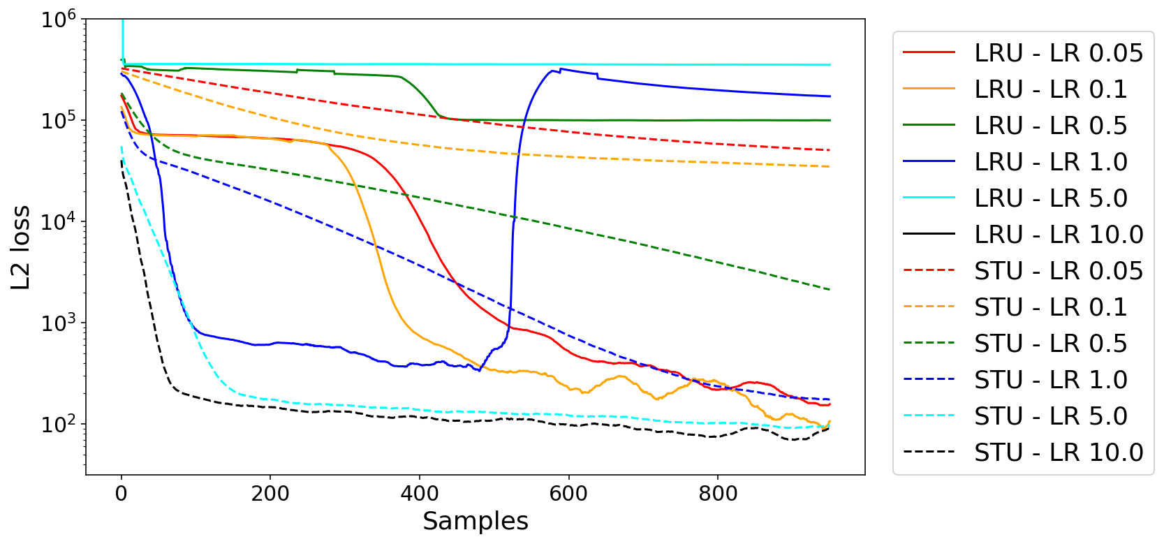
Figure 6: (Smoothed) Learning curves for learning a marginally stable LDS for a single STU layer (dashed) vs a single LRU layer (solid). Different colors represent different learning rates highlighting that the training becomes unstable for LRUs quickly as LR increases while the STU trains at much higher learning rates. Curiously at stable LRs we observe that LRUs show a platea-ing of learning for a large fraction of the training time.

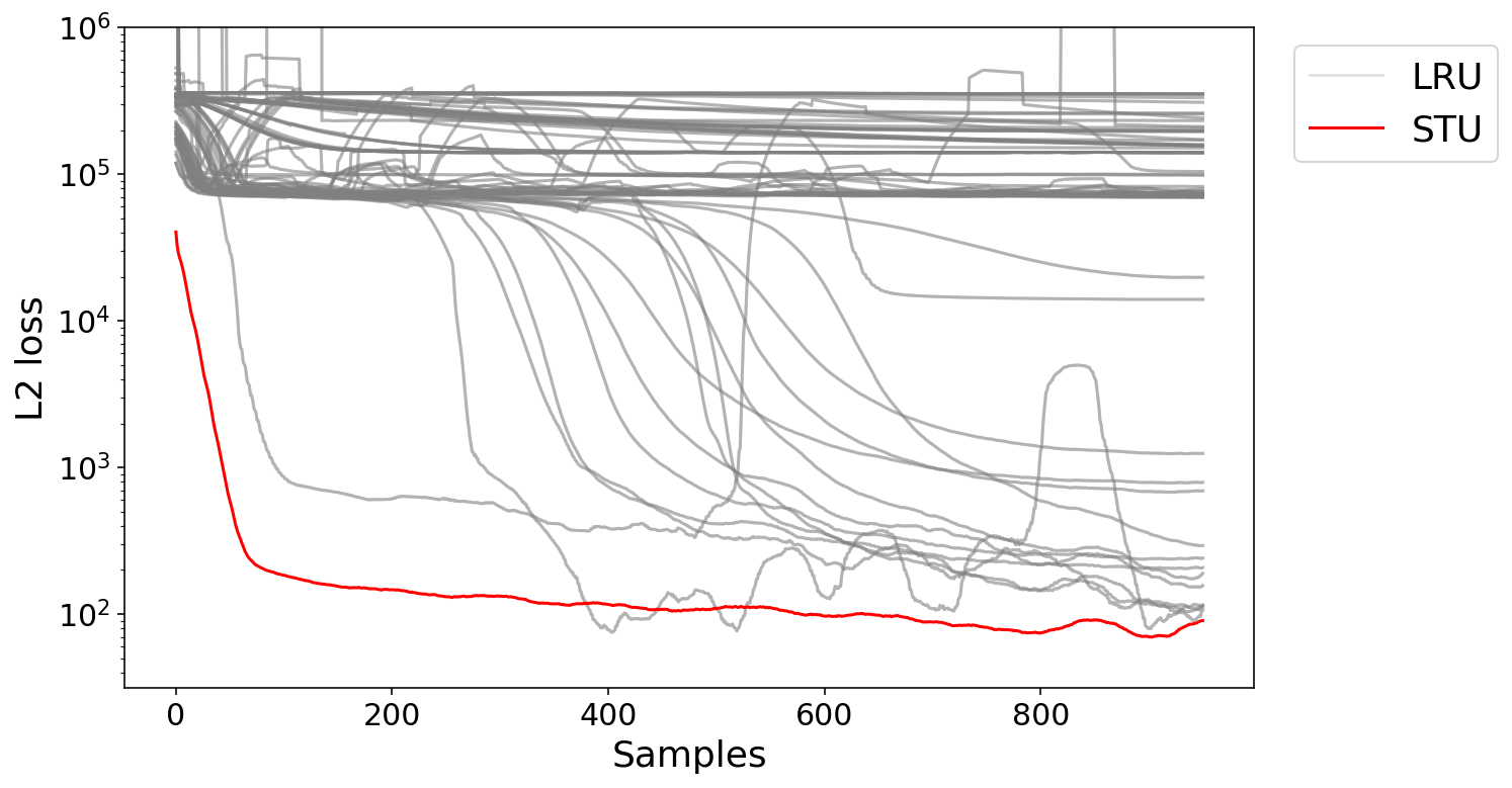
Figure 7: LRU Hparam search vs STU. All the gray curves represent the hyperparameters for LRU we tried. The STU curve is the best taken from Figure 6. For LRU we searched over choices of enabling stable exp-parameterization, gamma-normalization, ring-initialization, phase-initialization, learning rate, weight decay and constant vs warmup+cosine decay lr schedule.

C.2 Experimental setup for LRA experiments

Our training setup closely follows the experimental setup used by Orvieto et al. (2023). We use the same batch sizes and training horizons for all the tasks as employed by Orvieto et al. (2023).

Hyperparameter tuning For all of our experiments on the LRA benchmark for both the vanilla STU model and the auto-regressive AR-STU model we tune the learning rate in the set $\{1e-4,3e-4,5e-4,1e-3,2.5e-3,5e-3\}$ and tune the weight decay in the set $\{1e-3,1e-2,1e-1\}$. We fix the number of filters $K$ to be $24$. We use Adam as the training algorithm with other optimization hyperparameters set to their default values. We use the same learning rate schedule as Orvieto et al. (2023), i.e. 10% warmup followed by cosine decay to 0. For the AR-STU model we used the default value of $k_{y}=2$ but also tried $k_{y}=32$ on certain workloads. In Table 3 we present a comparison of performance gains afforded by $k_{y}=32$ where applicable.

Initialization For the STU model we initialized the $M$ matrices at 0. We found random initialization to also perform similarly. For the AR-STU model we initialize the $M^{y}$ matrices such that at initialization the model mimics the standard STU model, i.e. $M^{y}_{2}=\alpha\cdot I$ and $M^{y}_{i}=0$ otherwise. We found setting $\alpha<1$ to be better with respect to stability of the overall model. We tried a couple of values for the $\alpha$ parameter such as $0.9,0.75$ but found it to have negligible impact on performace. We suggest using either of these values.

Finally while training the AR-STU model as employed by the training setup of (Orvieto et al., 2023) we found using a smaller value of LR specifically for $M^{y}$ matrices to be useful. We decreased the value of LR by a factor $0.1$ or $0.05$ and tuned over this parameter.

	CIFAR	ListOps	Text	Retrieval	Pathfinder	PathX
AR-STU ($k_{y}=2$)	85.7	60.33	89.6	90.0	94.15	89.9
AR-STU ($k_{y}=32$)	91.3	–	–	–	95.6	–

Table 3: Comparison of $k_{y}=2$ and $k_{y}=32$ for AR-STU

Appendix D Power of Auto-regression: Dimension-dependent representation for LDS

In this section we give a short proof that any partially-observed LDS can be perfectly predicted via a linear predictor acting over at most $d$ of its past inputs and outputs where $d$ is the hidden-state dimensionality (i.e. $A\in{\mathbb{R}}^{d\times d}$). In particular

Theorem D.1.

Given an LDS parameterized by $A\in{\mathbb{R}}^{d\times d},B,C,D$, there exist coefficients $\alpha_{1:d}$ and matrices $\Gamma_{0:d}$ such that given any input sequence $u_{1:L}$, the output sequence $y_{1:L}$ generated by the action of the LDS on the input satisfies for all $t$

$$y_{t}=\sum_{i=1}^{d}\alpha_{i}y_{t-i}+\sum_{i=0}^{d}\Gamma_{i}u_{t-i}$$

Proof.

By unrolling the LDS we have that $y_{t}=\sum_{i=0}^{t}CA^{i}Bu_{t-i}+Du_{t}.$. By the Cayley Hamilton theorem, the matrix $A$ has a characteristic polynomial $p$ of degree $d$, namely there exists $d$ numbers $c_{1:d}$ such that

$$p(z)=\sum_{i=0}^{d}c_{i}z^{i}$$

satisfies $p(A)=0$. Without loss of generality we can assume the constant term in the polynomial is 1. We can now consider the series for $y_{t},y_{t-1},...$ as

$$\begin{matrix}y_{t}-Du_{t}&=&CBu_{t}&CABu_{t-1}&...&CA^{t}Bu_{1}\\ y_{t-1}-Du_{t-1}&=&0&CBu_{t-1}&...&CA^{t-1}Bu_{1}\\ \vdots\\ y_{t-d}-Du_{t-d}&=&0&0&...&CA^{t-d}Bu_{1}\\ \end{matrix}$$

Now, if we take the combination of the above rows according to the coefficients of the characteristic polynomial, we get that

$$\sum_{i=0}^{d}c_{i}y_{t-i}=\sum_{j=0}^{t}R_{j}+\sum_{i=0}^{d}Du_{t-i}$$ (9)

where $R_{j}$ is the appropriate sum along the $j^{\prime}th$ column of the matrix above. For all $j>d$, this amounts to an expression of the form:

$$j>d\ \ \Rightarrow\ \ R_{j}=\sum_{i=0}^{d}c_{i}CA^{i}\cdot A^{t-j}Bu_{t-j}=C(\sum_{i=0}^{d}c_{i}A^{i})\cdot A^{t-j}Bu_{t-j}=C\cdot p(A)\cdot A^{t-j}Bu_{t-j}=0.$$

Since all but the first $d$ columns are zero, rearranging (9) and collecting terms, we get that there exists coefficients $\alpha_{1:d}$ and matrices $\Gamma_{0:d}$ such that

$$y_{t}=\sum_{i=1}^{d}\alpha_{i}y_{t-i}+\sum_{j=0}^{d}\Gamma_{j}u_{t-j}.$$

∎

References

- Arjovsky et al. (2016) Arjovsky, M., Shah, A., and Bengio, Y. Unitary evolution recurrent neural networks. In International conference on machine learning, pp. 1120–1128. PMLR, 2016.
- Bengio et al. (1994) Bengio, Y., Simard, P., and Frasconi, P. Learning long-term dependencies with gradient descent is difficult. IEEE transactions on neural networks, 5(2):157–166, 1994.
- Blelloch (1989) Blelloch, G. E. Scans as primitive parallel operations. IEEE Transactions on computers, 38(11):1526–1538, 1989.
- Brown et al. (2020) Brown, T., Mann, B., Ryder, N., Subbiah, M., Kaplan, J. D., Dhariwal, P., Neelakantan, A., Shyam, P., Sastry, G., Askell, A., et al. Language models are few-shot learners. Advances in neural information processing systems, 33:1877–1901, 2020.
- Cho et al. (2014) Cho, K., Van Merriënboer, B., Gulcehre, C., Bahdanau, D., Bougares, F., Schwenk, H., and Bengio, Y. Learning phrase representations using rnn encoder-decoder for statistical machine translation. arXiv preprint arXiv:1406.1078, 2014.
- Dao et al. (2022) Dao, T., Fu, D. Y., Saab, K. K., Thomas, A. W., Rudra, A., and Ré, C. Hungry hungry hippos: Towards language modeling with state space models. arXiv preprint arXiv:2212.14052, 2022.
- Dosovitskiy et al. (2020) Dosovitskiy, A., Beyer, L., Kolesnikov, A., Weissenborn, D., Zhai, X., Unterthiner, T., Dehghani, M., Minderer, M., Heigold, G., Gelly, S., et al. An image is worth 16x16 words: Transformers for image recognition at scale. arXiv preprint arXiv:2010.11929, 2020.
- Elman (1990) Elman, J. L. Finding structure in time. Cognitive science, 14(2):179–211, 1990.
- Fu et al. (2023) Fu, D. Y., Epstein, E. L., Nguyen, E., Thomas, A. W., Zhang, M., Dao, T., Rudra, A., and Ré, C. Simple hardware-efficient long convolutions for sequence modeling. arXiv preprint arXiv:2302.06646, 2023.
- Ghai et al. (2020) Ghai, U., Lee, H., Singh, K., Zhang, C., and Zhang, Y. No-regret prediction in marginally stable systems. In Conference on Learning Theory, pp. 1714–1757. PMLR, 2020.
- Goel et al. (2022) Goel, K., Gu, A., Donahue, C., and Ré, C. It’s raw! audio generation with state-space models. In International Conference on Machine Learning, pp. 7616–7633. PMLR, 2022.
- Gu & Dao (2023) Gu, A. and Dao, T. Mamba: Linear-time sequence modeling with selective state spaces. arXiv preprint arXiv:2312.00752, 2023.
- Gu et al. (2020) Gu, A., Dao, T., Ermon, S., Rudra, A., and Ré, C. Hippo: Recurrent memory with optimal polynomial projections. In Larochelle, H., Ranzato, M., Hadsell, R., Balcan, M., and Lin, H. (eds.), Advances in Neural Information Processing Systems, volume 33, pp. 1474–1487. Curran Associates, Inc., 2020.
- Gu et al. (2021a) Gu, A., Goel, K., and Ré, C. Efficiently modeling long sequences with structured state spaces. arXiv preprint arXiv:2111.00396, 2021a.
- Gu et al. (2021b) Gu, A., Johnson, I., Goel, K., Saab, K., Dao, T., Rudra, A., and Ré, C. Combining recurrent, convolutional, and continuous-time models with linear state space layers. Advances in neural information processing systems, 34:572–585, 2021b.
- Gupta et al. (2022) Gupta, A., Gu, A., and Berant, J. Diagonal state spaces are as effective as structured state spaces. In Oh, A. H., Agarwal, A., Belgrave, D., and Cho, K. (eds.), Advances in Neural Information Processing Systems, 2022. URL https://openreview.net/forum?id=RjS0j6tsSrf.
- Hazan & Singh (2022) Hazan, E. and Singh, K. Introduction to online nonstochastic control. arXiv preprint arXiv:2211.09619, 2022.
- Hazan et al. (2017) Hazan, E., Singh, K., and Zhang, C. Learning linear dynamical systems via spectral filtering. In Advances in Neural Information Processing Systems, pp. 6702–6712, 2017.
- Hazan et al. (2018) Hazan, E., Lee, H., Singh, K., Zhang, C., and Zhang, Y. Spectral filtering for general linear dynamical systems. In Advances in Neural Information Processing Systems, pp. 4634–4643, 2018.
- Hochreiter & Schmidhuber (1997) Hochreiter, S. and Schmidhuber, J. Long short-term memory. Neural computation, 9(8):1735–1780, 1997.
- Hopfield (1982) Hopfield, J. J. Neural networks and physical systems with emergent collective computational abilities. Proceedings of the national academy of sciences, 79(8):2554–2558, 1982.
- Jumper et al. (2021) Jumper, J., Evans, R., Pritzel, A., Green, T., Figurnov, M., Ronneberger, O., Tunyasuvunakool, K., Bates, R., Žídek, A., Potapenko, A., et al. Highly accurate protein structure prediction with alphafold. Nature, 596(7873):583–589, 2021.
- Li et al. (2022) Li, Y., Cai, T., Zhang, Y., Chen, D., and Dey, D. What makes convolutional models great on long sequence modeling? arXiv preprint arXiv:2210.09298, 2022.
- Orvieto et al. (2023) Orvieto, A., Smith, S. L., Gu, A., Fernando, A., Gulcehre, C., Pascanu, R., and De, S. Resurrecting recurrent neural networks for long sequences. arXiv preprint arXiv:2303.06349, 2023.
- Pascanu et al. (2013) Pascanu, R., Mikolov, T., and Bengio, Y. On the difficulty of training recurrent neural networks. In International conference on machine learning, pp. 1310–1318. Pmlr, 2013.
- Poli et al. (2023) Poli, M., Massaroli, S., Nguyen, E., Fu, D. Y., Dao, T., Baccus, S., Bengio, Y., Ermon, S., and Ré, C. Hyena hierarchy: Towards larger convolutional language models. arXiv preprint arXiv:2302.10866, 2023.
- Rumelhart et al. (1985) Rumelhart, D. E., Hinton, G. E., Williams, R. J., et al. Learning internal representations by error propagation, 1985.
- Shi et al. (2023) Shi, J., Wang, K. A., and Fox, E. Sequence modeling with multiresolution convolutional memory. In International Conference on Machine Learning, pp. 31312–31327. PMLR, 2023.
- Simchowitz et al. (2018) Simchowitz, M., Mania, H., Tu, S., Jordan, M. I., and Recht, B. Learning without mixing: Towards a sharp analysis of linear system identification. In Conference On Learning Theory, pp. 439–473. PMLR, 2018.
- Smith et al. (2023) Smith, J. T., Warrington, A., and Linderman, S. Simplified state space layers for sequence modeling. In The Eleventh International Conference on Learning Representations, 2023.
- Tay et al. (2021) Tay, Y., Dehghani, M., Abnar, S., Shen, Y., Bahri, D., Pham, P., Rao, J., Yang, L., Ruder, S., and Metzler, D. Long range arena : A benchmark for efficient transformers. In International Conference on Learning Representations, 2021. URL https://openreview.net/forum?id=qVyeW-grC2k.
- Tay et al. (2022) Tay, Y., Dehghani, M., Bahri, D., and Metzler, D. Efficient transformers: A survey. ACM Comput. Surv., 55(6), dec 2022. ISSN 0360-0300. doi: 10.1145/3530811. URL https://doi.org/10.1145/3530811.
- Vaswani et al. (2017) Vaswani, A., Shazeer, N., Parmar, N., Uszkoreit, J., Jones, L., Gomez, A. N., Kaiser, Ł., and Polosukhin, I. Attention is all you need. Advances in neural information processing systems, 30, 2017.
- Zhang et al. (2023) Zhang, M., Saab, K. K., Poli, M., Dao, T., Goel, K., and Ré, C. Effectively modeling time series with simple discrete state spaces. arXiv preprint arXiv:2303.09489, 2023.