A local study of dynamo action driven by precession

Abstract

We demonstrate an efficient magnetic dynamo due to precession-driven hydrodynamic turbulence in the local model. Dynamo growth rate increases with Poincaré and magnetic Prandtl numbers. Spectral analysis shows that the dynamo acts over a broad range of scales: at large (system size) and intermediate scales it is driven by 2D vortices and shear of the background precessional flow, while at smaller scales it is mainly driven by 3D inertial waves. These results are important for understanding magnetic field generation and amplification in precessing planets and stars.

Understanding the generation, amplification and self-sustenance of magnetic fields in astrophysical and geophysical objects is the endeavour of dynamo theory Roberts (1994); Moffatt and Dormy (2019). From the magnetic field of our planet to distant stars and galaxies, magnetohydrodynamic (MHD) dynamo models offer insights into complex interplay between flows of conducting fluids and fields, leading to the growth of the latter. To achieve this, dynamo must be sufficiently efficient in transforming kinetic energy of a flow into magnetic energy, which in turn requires a strong driving mechanism of the flow.

Among the known driving mechanisms for planetary dynamos, precession-powered motion is a complementary candidate Malkus (1968); Vanyo (1991) to a more generally accepted convection Landeau et al. (2022). Precession takes place when the rotation axis of a system changes its orientation, producing a volume force that drives a flow in the (liquid) interior of the precessing body Lagrange et al. (2011). Precession-driven flows are potentially able to convert large amounts of kinetic energy (up to $10^{11}-10^{21}$ W Loper (1975); Rochester et al. (1975); Vanyo (1991)) to sustain the geomagnetic field Malkus (1968). This conversion is due to instabilities Lagrange et al. (2011); Giesecke et al. (2015) that give rise to vortex tangles and may also induce turbulence within superfluid neutron stars Glampedakis et al. (2008, 2009).

Precession-driven flows have been studied both numerically Tilgner (2005); Giesecke et al. (2018); Pizzi et al. (2021, 2021); Cébron et al. (2019); Kong et al. (2015); Goepfert and Tilgner (2016); Lin et al. (2016) and experimentally Noir et al. (2001); Meunier et al. (2008); Goto et al. (2014); Kumar et al. (2023) and their ability to drive dynamo was demonstrated for laboratory flows in a specific parameter regime Giesecke et al. (2018); Kumar et al. (2023). In astrophysics and geophysics, precessing flows are studied using a widely employed local model Mason and Kerswell (2002); Barker (2016); Khlifi et al. (2018); Pizzi et al. (2022a), which describes a small segment of a celestial body (stars, gaseous planets or the liquid cores of rocky planets) in a Cartesian coordinate frame $(x,y,z)$ rotating around the $z$-axis and precessing around another tilted axis with angular velocities $\Omega$ and ${\rm Po}\cdot\Omega$, respectively, where ${\rm Po}$ is Poincaré number characterizing precession strength. In this local frame, the precession-driven flow has a linear shear along the vertical $z$-axis, which oscillates in time and is proportional to $\rm Po$, $\bm{U}_{0}=-2\Omega\cdot{\rm Po}\cdot z(\sin(\Omega t),\cos(\Omega t),0)^{T}$ Mason and Kerswell (2002); Barker (2016); Pizzi et al. (2022a). This background flow is subject to a precessional instability and breaks down into a nonlinear (turbulent) state consisting of 2D vortices and 3D inertial waves Barker (2016); Khlifi et al. (2018); Pizzi et al. (2022a).

In this Letter, following our hydrodynamical study Pizzi et al. (2022a), we consider the MHD case and demonstrate a magnetic dynamo action powered by the precession-driven turbulence resulting from the nonlinear saturation of the precessional instability. Previous studies Tilgner (2005); Goepfert and Tilgner (2016); Lin et al. (2016); Cébron et al. (2019); Giesecke et al. (2018); Pizzi et al. (2022b) on the precession dynamo in global settings, mostly in the context of laboratory experiments, emphasized the significance of large-scale vortices as a primary driver for large-scale magnetic field amplification, suggesting that the nature of the dynamo is closely linked to this flow pattern. This work, going beyond those findings, demonstrates for the first time the strong influence of the precession on the dynamo properties over a much broader range of scales not captured in the current global models. Focusing on the kinematic stage, we show a remarkable transition from a vortex-driven large-scale dynamo at small $\rm Po$ to a more complex type driven both by vortices and waves at different scales at higher ${\rm Po}$. These two regimes of the dynamo are governed by the intrinsic dynamics of precession-driven flows, namely their transition from the dominant geostrophic vortices to 3D inertial wave turbulence with increasing $\rm Po$ Pizzi et al. (2022a).

Consider a velocity perturbation $\bm{u}$ about the background flow $\bm{U}_{0}$ in the rotating and precessing frame. The main MHD equations for a conducting incompressible fluid in this local frame are Barker (2016); Pizzi et al. (2022a)

$$(\partial_{t}+\bm{U}_{0}\cdot\bm{\nabla}+\bm{u}\cdot\bm{\nabla})\bm{u}=-\frac{1}{\rho}\bm{\nabla}\Pi+\frac{1}{\rho}(\bm{B}\cdot\bm{\nabla})\bm{B}+\nu\bm{\nabla}^{2}\bm{u}-\\ 2\Omega\bm{e}_{z}\times\bm{u}-2\Omega\bm{\varepsilon}(t)\times\bm{u}+2\Omega u_{z}\bm{e}_{z}\times\bm{\varepsilon}(t),$$ (1)

$$(\partial_{t}+\bm{U}_{0}\cdot\bm{\nabla})\bm{B}=\nabla\times(\bm{u}\times\bm{B})+\eta\bm{\nabla}^{2}\bm{B}-2\Omega B_{z}\bm{e}_{z}\times\bm{\varepsilon}(t),$$ (2)

supplemented with $\bm{\nabla}\cdot\bm{u}=\bm{\nabla}\cdot\bm{B}=0$, where $\rho$ is the constant density of the fluid, $\Pi$ is the sum of thermal and magnetic pressures, $\bm{B}$ is the magnetic field, $\nu$ is the kinematic viscosity, $\eta$ is the magnetic diffusivity and the vector $\bm{\varepsilon}(t)={\rm Po}(\cos(\Omega t),-\sin(\Omega t),0)^{T}$ describes the effects of precession in these equations. Specifically, Coriolis acceleration due to precession, $-2\Omega\bm{\varepsilon}(t)\times\bm{u}$, and the stretching term $2\Omega u_{z}\bm{e}_{z}\times\bm{\varepsilon}(t)$ of the perturbation velocity due to the shear of the base flow in Eq. (1) jointly give rise to the precessional instability Kerswell (1993); Salhi et al. (2010). A similar stretching term $-2\Omega B_{z}\bm{e}_{z}\times\bm{\varepsilon}(t)$ in Eq. (2) describes the growth of the magnetic field due to the shear.

The flow is considered in a periodic cubic box with the length $L$ in each direction, $L_{x}=L_{y}=L_{z}=L$. We normalize time by $\Omega^{-1}$, length by $L$, velocity by $\Omega L$ and pressure as well as kinetic $E_{v}=\rho\bm{u}^{2}/2$ and magnetic $E_{m}=\bm{B}^{2}/2$ energy densities by $\rho L^{2}\Omega^{2}$. The main parameters are the Poincaré, ${\rm Po}$, the Reynolds, ${\rm{Re}}=\Omega L^{2}/\nu$, and magnetic Prandtl, ${\rm{Pm}}=\nu/\eta$, numbers. Below we fix ${\rm Re}=3\times 10^{4}$ and explore a broad range of ${\rm Po}=0.075-0.4$ and ${\rm Pm}=10^{-1}-10$.

We solve Eqs. (1) and (2) using the spectral code SNOOPY Lesur and Longaretti (2005) adapted to the local precessional flow Barker (2016). Resolution for $\rm Pm<1$, i.e., when the viscous scales are shortest, is set as in Pizzi et al. (2022a): $(N_{x},N_{y},N_{z})=(128,128,128)$ at $\rm Po\leq 0.125$ and $(256,256,256)$ at $\rm Po>0.125$, while for $\rm Pm>1$, when resistive scales are shortest instead, it is increased by a factor ${\rm Pm}^{1/2}$. Random velocity perturbations with rms $\left<\bm{u}^{2}\right>^{1/2}=1.12\times 10^{-4}$ and a very weak random magnetic field with rms $\left<\bm{B}^{2}\right>^{1/2}=10^{-12}$, are imposed initially, so that the back-reaction of the magnetic field on the flow is negligible.

Figure 1 shows the evolution of the volume-averaged kinetic $\left<E_{v}\right>$ and magnetic $\left<E_{m}\right>$ energies at different $\rm Po$ and $\rm Pm$, which indicates a two-staged dynamo process. In the beginning, the kinetic energy grows exponentially as a result of the linear precessional instability, while the magnetic energy decreases. After several precession times $\sim(\epsilon\Omega)^{-1}$, the exponential growth saturates due to nonlinearity [advection ($\bm{u}\cdot\bm{\nabla})\bm{u}$ in Eq. (1)] and the flow settles down into a quasi-steady turbulence composed of 2D vortices and 3D inertial waves Barker (2016); Pizzi et al. (2022a). Remarkably, the dynamo action – exponential growth of the magnetic field – starts only after saturation of the precession instability and is driven by the nonlinear (turbulent) velocity perturbations. After several hundred orbits, the magnetic field growth saturates nonlinearly due to the back-reaction of Lorentz force on the flow, which is discernible by the small drop in $\left<E_{v}\right>$ at the saturation point of $\left<E_{m}\right>$ (Fig. 1). The growth rate of the magnetic energy, $\gamma=d~{}{\rm ln}\langle E_{m}\rangle/dt$, in the kinematic regime and its nonlinear saturation level increase, and hence the dynamo is more efficient, with increasing $\rm Po$ and/or $\rm Pm$. This dependence on $\rm Po$ and $\rm Pm$ is further explored in Fig. 2, which shows $\gamma$ in the $(\rm{Po,Pm})$-plane and summarizes all our runs. Note that the critical $\rm Po_{c}$ for the dynamo onset decreases with increasing $\rm Pm$.

Figure 3 shows the structures of the vertical vorticity $\omega_{z}=(\nabla\times\bm{u})_{z}$ in physical space at $\rm Po=0.15$ and, at the same instants, the induced vertical field $B_{z}$ during the kinematic stage in two runs at $\rm Pm=3$ and $7$. We observe vertically nearly uniform larger-scale columnar vortices embedded in a sea of smaller-scale 3D inertial waves, as typical of precession-driven turbulence Barker (2016); Khlifi et al. (2018); Pizzi et al. (2022a). The traces of these vortices are visible in the magnetic field, since vortices are in fact the main drivers of the dynamo at this small $\rm Po$ (see Fig. 5). Note the decrease in characteristic length of $B_{z}$ structures as $\rm Pm$ increases.

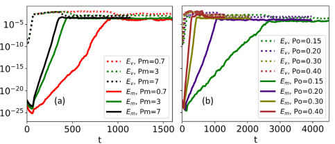
Figure 1: Evolution of the volume-averaged kinetic $\left<E_{v}\right>$ (dotted) and magnetic $\left<E_{m}\right>$ (solid) energies at $\rm Re=3\times 10^{4}$ for (a) different $\rm Pm$ at $\rm Po=0.3$ and (b) different $\rm Po$ at $\rm Pm=3$.

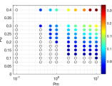
Figure 2: Dynamo growth rate $\gamma$ in the ${\rm(Pm,Po)}-$plane indicated by color points, whereas there is no dynamo at empty points. Both color and empty points represent all the simulations done.

To analyse dynamo action across length-scales, we decompose the magnetic field into Fourier modes Barker (2016); Pizzi et al. (2022a)

$$\bm{B}\left(\bm{r},t\right)=\sum_{\bm{k}}\bar{\bm{B}}\left(\bm{k}(t),t\right)e^{i\bm{k}(t)\cdot\bm{r}},$$ (3)

where $\bm{k}(t)=(k_{x},~{}k_{y},~{}k_{z}(t))^{T}$ is the wavevector with $k_{z}(t)=k_{z0}+2{\rm Po}(-k_{x}{\rm cos}(t)+k_{y}{\rm sin}(t))$ oscillating in time about a constant $k_{z0}$ due to the periodic time-variation of the background flow $\bm{U}_{0}$.

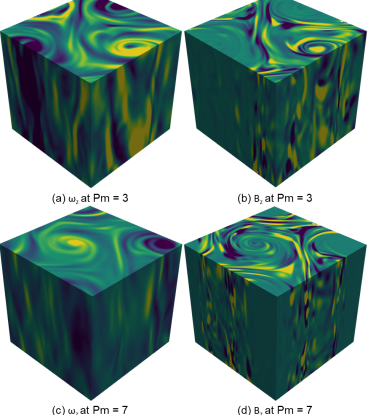
Figure 3: Spatial structures of the vertical vorticity $\omega_{z}=(\nabla\times\bm{u})_{z}$ at $\rm Po=0.15$ in two runs at (a) $\rm Pm=3$ and (c) $\rm Pm=7$ alongside the corresponding induced vertical field $B_{z}$ in (b) and (d), respectively. For each $\rm Pm$, the snapshots of $\omega_{z}$ and $B_{z}$ are shown at equal instants during the kinematic regime.

Figure 4 shows the shell-averaged magnetic energy spectrum, ${\cal E}_{m}=|\bar{\bm{B}}|^{2}/2$, in the middle of and at the end of the kinematic stage together with the corresponding growth rate $\gamma(k)$ versus wavenumber $k=|\bm{k}|$ at different $\rm Po$ and $\rm Pm$. Note that in all the cases, the growth rate is nearly constant and positive, $\gamma(k)>0$, at lower and intermediate $k\lesssim 200$, indicating the dynamo action at these wavenumbers, and decreases, turning negative, at higher $k$ due to resistivity. At small $\rm Po=0.15$, the growth rate weakly increases with $\rm Pm$, mostly at higher wavenumbers [Fig. 4(a)]. As a result, the energy spectra at $\rm Pm=3$ and 7 have nearly the same shape and magnitude at small and intermediate wavenumbers, both during and at the end of the growth, while high wavenumbers have more power for $\rm Pm=7$ than that for $\rm Pm=3$. The magnetic energy spectrum and $\gamma(k)$ depend more strongly on $\rm Pm$ at higher $\rm Po=0.3$ and 0.4, as seen in Figs. 4(b) and 4(c), respectively. For a given $\rm Po$, the positive growth rate (nearly independent of $k$ at lower $k$) increases with $\rm Pm$ and extends to higher $k$’s the larger $\rm Pm$ is, so the spectrum grows faster at high $k$ with increasing $\rm Pm$ and hence is less steep.

Figure 4: (Top row) Shell-averaged magnetic energy spectra in the middle (dashed) and at the end (solid) of the kinematic stage of the dynamo at various $\rm Pm$ for (a) $\rm Po=0.15$, (b) 0.3 and (c) 0.4. (Bottom row) The corresponding growth rate $\gamma(k)$ of the spectral magnetic energy. There is no dynamo at $\rm Po=0.15$ and $\rm Pm=0.7$, hence the yellow curve is absent in panel (a).

Comparing now the spectral behavior for different $\rm Po$ and given $\rm Pm$ in Fig. 4, we notice that with increasing $\rm Po$, $\gamma(k)$ moderately increases, although the maximum $k$ where there is still a dynamo does not appear to change much from $\rm Pm=0.7$ to 3. This threshold wavenumber increases with $\rm Po$ at higher $\rm Pm=7$, being associated with driving by small-scale waves at high $k$ (see below). As a result, the magnetic energy spectra are shallower at high $k$ for $\rm Po=0.4$ and 0.3 than those for $\rm Po=0.15$.

The precession-driven hydrodynamic turbulence, as noted above, consists of 2D vortices and 3D inertial waves Barker (2016); Khlifi et al. (2018); Pizzi et al. (2022a) similar to classical (forced) rotating turbulence Buzzicotti et al. (2018); Alexakis and Biferale (2018). The slow 2D vortical mode varies only in the horizontal $(x,y)$-plane and is uniform along the $z$-axis, having $k_{z}=0$. The velocity of this mode, denoted as $\bm{u}_{2D}$, has the dominant horizontal component $u_{h}=(u_{x}^{2}+u_{y}^{2})^{\nicefrac{{1}}{{2}}}\gg u_{z}$. On the other hand, the fast 3D inertial wave mode with nonzero frequency $\pm 2\Omega k_{z}/k$, varies along the $z$-axis, $k_{z}\neq 0$, and its velocity $\bm{u}_{3D}$ has comparable horizontal and vertical components, $u_{h}\sim u_{z}$. We will show that these modes play a crucial role in the dynamo action and its dependence on ${\rm{Po}}$.

To understand the roles of the background flow $\bm{U}_{0}$ as well as the vortices and inertial waves in driving the precession dynamo, we first obtain the equation for the magnetic energy spectrum ${\cal E}_{M}$ by substituting transformation (3) into Eq. (2) and multiplying by conjugate $\bar{\bm{B}}^{\ast}$. Then, in the electromotive force (EMF) $\nabla\times(\bm{u}\times\bm{B})$, the velocity is divided into vortical $\bm{u}_{2D}$ and wave $\bm{u}_{3D}$ components, $\bm{u}=\bm{u}_{2D}+\bm{u}_{3D}$, giving

$$\frac{d{\cal E}_{M}}{dt}=P+D_{M}+I_{2D}+I_{3D},$$ (4)

where $P=\Omega(\bar{\bm{B}}^{\ast}\bar{B}_{z}+\bar{\bm{B}}\bar{B}_{z}^{\ast})(\bm{\varepsilon}(t)\times\bm{e}_{z})$ describes energy exchange between magnetic field and the background flow due to shear; when $P>0$ energy is injected from the flow into the field. The second term $D_{M}=-2k^{2}{\cal E}_{M}/(Re\cdot Pm)<0$ is resistive dissipation. The third $I_{2D}$ and fourth $I_{3D}$ terms related to $\bm{u}_{2D}$ and $\bm{u}_{3D}$ in the Fourier transform of EMF (denoted with bar) are given by $I_{2D}={\rm i}[\bar{\bm{B}}^{\ast}\bm{k}\times\overline{(\bm{u}_{2D}\times\bm{B})}-\bar{\bm{B}}\bm{k}\times\overline{(\bm{u}_{2D}\times\bm{B})}^{\ast}]/2$ and $I_{3D}={\rm i}[\bar{\bm{B}}^{\ast}\bm{k}\times\overline{(\bm{u}_{3D}\times\bm{B})}-\bar{\bm{B}}\bm{k}\times\overline{(\bm{u}_{3D}\times\bm{B})}^{\ast}]/2$ and describe magnetic energy production, respectively, by vortices and inertial waves.

Figure 5: Shell-averaged spectra of the dynamical terms in Eq. (4): energy injection from the flow, $P$, resistive dissipation, $D_{M}$, and the contributions from 2D vortices, $I_{2D}$, and 3D inertial waves, $I_{3D}$, in the middle of the kinematic stage at (a) Po = 0.15, Pm = 3; (b) Po = 0.15, Pm = 7; (c) Po = 0.3, Pm = 3 and (d) Po = 0.3, Pm = 7.

Figure  5 shows the shell-averaged spectra of these four terms in the middle of the kinematic stage. Depending on $\rm Po$ and $\rm Pm$, either only vortices, or cooperatively vortices and waves are mainly responsible for the magnetic field amplification. At the lowest $\rm Po=0.15$, both for $\rm Pm=3$ and $7$, the dynamo is mainly driven by vortices, because $I_{2D}$ is positive and much larger than $I_{3D}$ and $P$ [Figs. 5(a) and 5(b)]. As $\rm Pm$ increases, $I_{2D}$ extends a bit to higher $k$, although its dependence on $\rm Pm$ seems to be weak at this $\rm Po$, consistent with the behavior in Fig. 4(a). At higher $\rm Po=0.3$ the role of inertial waves in driving the dynamo becomes more appreciable: $I_{3D}$ is now comparable to $I_{2D}$ and $P$, but mostly operates at higher $k\gtrsim 100$ than the latter two terms (since the relevant waves are of small-scale), as seen in Figs. 5(c) and 5(d) for the same $\rm Pm$. With increasing $\rm Pm$, $I_{3D}$ dominates over $I_{2D}$ and $P$ at large $k$, so the 3D waves become the main drivers of the dynamo at small scales, while the vortices and injection from the base flow dominate at lower $k$, i.e., larger scales [Fig. 5(d)].

To conclude, we revealed and analyzed dynamo action powered by precession-driven turbulence, which is capable of exponentially amplifying magnetic field. Although our model is local, it captures two basic ingredients of the turbulence: large-scale 2D vortices and smaller-scale 3D inertial waves. This model covers thus a broader range of length-scales – from the system size to the shortest dissipation scales – than existing global models of precessional flows Tilgner (2005); Giesecke et al. (2018); Pizzi et al. (2021, 2021); Cébron et al. (2019); Kong et al. (2015); Goepfert and Tilgner (2016); Lin et al. (2016), thereby providing deeper insights into the precession dynamo properties (growth rate, energy spectra, driving mechanism) over these scales. We showed that during the kinematic stage, the growth rate of the dynamo increases with the Poincaré ($\rm Po$) and the magnetic Prandtl ($\rm Pm$) numbers. The critical $\rm Pm_{c}$ for the dynamo onset also increases with decreasing $\rm Po$. At small $\rm Po\lesssim 0.15$ the dynamo is mainly driven by 2D vortices at large (system size) and intermediate scales, being therefore less sensitive to ${\rm Pm}$. At larger $\rm Po\gtrsim 0.15$, driving by waves at smaller scales becomes important and hence the dynamo growth rate increases with $\rm Pm$ and $\rm Po$, while at larger scales the dynamo is still driven by 2D vortices and the shear of the background precessional flow.

Finally, we note the sequence of processes leading to the dynamo action here (a precessional flow subject to instability $\rightarrow$ turbulence $\rightarrow$ vortices $\rightarrow$ dynamo) resembles that taking place in rotating convection. As shown in Guervilly et al. (2015), thermal convection in the presence of rotation leads to turbulence and formation of large-scale vortices, which in turn amplify large-scale magnetic field. Thus, these two different (convection and precession) processes share a common generic mechanism – vortex-induced dynamo, which we have analyzed here. Thus, this study can be important not only for understanding the magnetic dynamo action in precessing planets and stars, but also in a more general context of flow systems where vortices emerge and govern the flow dynamics.