Gravitational Rényi entropy from corner terms

Abstract

We provide a consistent first principles prescription to compute gravitational Rényi entropy using Hayward corner terms. For Euclidean solutions to Einstein gravity, we compute Rényi entropy of Hartle–Hawking and fixed–area states by cutting open a manifold containing a conical singularity into a wedge with a corner. The entropy functional for fixed–area states is equal to the corner term itself, having a flat-entanglement spectrum, while extremization of the functional follows from the variation of the corner term under diffeomorphisms. Notably, our method does not require regularization of the conical singularity, and naturally extends to higher-curvature theories of gravity.

Introduction. Gravity has an information theoretic character. Evidence for this is captured by the Ryu–Takayanagi prescription for computing entanglement entropy of holographic conformal field theories (CFT) [1, 2],

$$S_{\text{EE}}(A)=\underset{\mathcal{C}\,\sim\,\partial A}{\text{min}}\frac{\text{Area}\,(\mathcal{C})}{4G_{\text{N}}}\;.$$ (1)

Namely, entanglement entropy of a holographic CFT state reduced to a (spatial) subregion $A$ of the boundary of anti-de Sitter (AdS) space equals the area of a bulk minimal surface $\mathcal{C}$ anchored to boundary $\partial A$ and homologous to $A$. The relation (1) generalizes the Bekenstein–Hawking entropy formula [3, 4, 5, 6], revealing surfaces other than horizons carry entropy. Further, a possible microscopic interpretation of gravitational entropy is that it measures entangled degrees of freedom of a dual CFT.

The prescription (1) has a well-known derivation at the level of the gravitational path integral [7]. To wit, consider a CFT living on the boundary $B$ of AdS. Then invoke the ‘replica trick’: glue together integer $n$-copies of $B$, producing an $n$-fold cover $B_{n}$ with partition function $Z[B_{n}]$. The entanglement entropy of a quantum state reduced to a boundary subregion $A$ is given by the analytic continuation $n\to 1$ of the $n$th Rényi entropy,

$$S_{\text{EE}}(A)=-\partial_{n}(\log Z[B_{n}]-n\log Z[B])|_{n=1}\;.$$ (2)

Via AdS/CFT, the boundary partition function $Z[B_{n}]$ may be evaluated in the saddle-point approximation by the on-shell action $I_{\mathcal{M}_{n}}[\mkern 1.5mu\overline{\mkern-1.5mug\mkern-1.5mu}\mkern 1.5mu_{n}]$ of a regular bulk solution $(\mathcal{M}_{n},\mkern 1.5mu\overline{\mkern-1.5mug\mkern-1.5mu}\mkern 1.5mu_{n})$ to the bulk field equations with boundary $B_{n}$. For Hartle–Hawking states (defined below) and assuming $\mkern 1.5mu\overline{\mkern-1.5mug\mkern-1.5mu}\mkern 1.5mu_{n}$ preserves the $\mathbb{Z}_{n}$ permutation symmetry of $n$-replicas, the entropy (2) can be computed by

$$S_{\text{EE}}(A)=\partial_{n}I_{\mathcal{M}_{n}/\,\mathbb{Z}_{n}}[\mkern 1.5mu\overline{\mkern-1.5mug\mkern-1.5mu}\mkern 1.5mu_{n}]\big{|}_{n=1}\;.$$ (3)

Here the orbifold $(\mathcal{M}_{n}/\,\mathbb{Z}_{n},\mkern 1.5mu\overline{\mkern-1.5mug\mkern-1.5mu}\mkern 1.5mu_{n})$ is regular everywhere except along a bulk codimension-2 surface $\mathcal{C}$ with a conical defect due to the fixed points of $\mathbb{Z}_{n}$. For Einstein gravity, (3) returns (1), where the area and its minimization are computed in the solution $(\mathcal{M},\mkern 1.5mu\overline{\mkern-1.5mug\mkern-1.5mu}\mkern 1.5mu)$ with boundary $B$ [7].

In this letter we present a new method of deriving gravitational entropy using a technique we call the ‘corner method’. Key to our approach is to recognize the conical singularity arising from the replica trick as a corner: a codimension-2 surface at the intersection of two codimension-1 boundaries. We cut open the conical singularity into a wedge whose boundaries meet at a corner, such that a Hayward corner term is required to have a well-posed variational problem [8]. This cutting has no effect on the value of the gravitational action, such that the Euclidean action of the wedge entirely encodes the gravitational entropy functional, and is consistent with the extremization prescription. Alternatively, our observation provides a rigorous definition of the action of a conical singularity that does not require regularization.

Historically, corner terms have been used to compute entropy of stationary black holes [9, 10, 11, 12]. i.e., solutions whose Euclideanization have a $U(1)$ Killing symmetry with the bifurcate Killing horizon being a fixed point of the $U(1)$ isometry. Our approach thus extends these computations to backgrounds without a $U(1)$ symmetry, analogous to how [7] generalizes the Gibbons–Hawking derivation of black hole thermodynamics [13].

There are three notable features of our approach. First, we directly compute entropy functionals and their extremization for Hartle–Hawking and fixed–area states. For fixed–area states, area minimization follows from varying the Einstein action of the wedge under transverse diffeomorphisms of the corner. Second, unlike derivations [7, 14], we need not regularize any conical singularity. Thirdly, our method extends to higher-curvature theories. In Lovelock gravity, for example, fixed–area states generalize to fixed Jacobson–Myers functional states, having a flat entanglement spectrum [15].

Set-up and gravitational states. While motivated by AdS/CFT, our approach applies more broadly. Let $(\mathcal{M},g)$ be a $D$-dimensional Riemannian manifold endowed with a Euclidean metric $g$, and $(B,\gamma)$ be its $(D-1)$-dimensional boundary with topology $B=S^{1}\times Y$ and metric $\gamma$. Another codimension-1 manifold $(B_{n},\gamma)$ is constructed by cutting and cyclically pasting together positive integer $n$-copies of $(B,\gamma)$ along $Y$. We will look for bulk solutions $(\mathcal{M}_{n},\mkern 1.5mu\overline{\mkern-1.5mug\mkern-1.5mu}\mkern 1.5mu)$ with boundary $(B_{n},\gamma)$. Further, let $\tau\in(0,2\pi)$ be the Euclidean time coordinate parametrizing the circle $S^{1}$. Then the cutting-gluing surgery extends this range to $\tau\in(0,2\pi n)$, keeping the metric $\gamma$ fixed in these coordinates. Moreover, $B_{n}$ has a $\mathbb{Z}_{n}$ replica symmetry owed to the cyclical gluing.

We define the (refined) gravitational Rényi entropy

$$\widetilde{S}_{n}\equiv(n\partial_{n}-1)\,I_{\mathcal{M}_{n}}[\mkern 1.5mu\overline{\mkern-1.5mug\mkern-1.5mu}\mkern 1.5mu]\;.$$ (4)

To determine the solution $\mkern 1.5mu\overline{\mkern-1.5mug\mkern-1.5mu}\mkern 1.5mu$, we must specify the gravitational state. We are interested in two types of states:

1. Hartle–Hawking (HH) states, prepared by a Euclidean gravity path integral over all metrics with fixed asymptotics at infinity.

2. Fixed–area states, prepared by a Euclidean gravity path integral over metrics with a given fixed area $\mathcal{A}$ on a codimension-2 surface $\mathcal{C}$ in the interior and fixed asymptotics at infinity.

More carefully, a fixed–area state is defined as follows [16]. Gauge-fix a Cauchy slice $\Sigma$ such that it passes through a codimension-2 surface $\mathcal{C}$ and fixes the location of $\mathcal{C}$ on $\Sigma$. This defines a state with $\mathcal{C}$ of fixed area $\mathcal{A}$. The associated bulk wavefunctional is found by restricting the Hartle-Hawking wavefunctional characterizing the HH state on a $\Sigma$ which gives $\mathcal{C}$ area $\mathcal{A}$. In the path integral this amounts to fixing the induced metric on $\Sigma$ to yield area $\mathcal{A}$ for $\mathcal{C}$ in addition to the same asymptotics.

Thus, gravitational states (i) and (ii) induce different boundary conditions at the codimension-2 surface $\mathcal{C}$ where the Euclidean time circle shrinks to zero size. In particular, let $\rho>0$ be a radial coordinate where $\mathcal{C}$ is located at $\rho=0$. For $\tau\sim\tau+2\pi n$, the boundary conditions associated to states (i) and (ii) result in the following metric expansions near $\mathcal{C}$:

1. Fixed-periodicity boundary condition

   $$ds^{2}=d\rho^{2}+\frac{\rho^{2}}{n^{2}}\,d\tau^{2}+\sigma_{AB}(\hat{x})\,d\hat{x}^{A}d\hat{x}^{B}+\ldots$$ (5)

   This boundary condition is used in the proof of prescription (1) by Lewkowycz and Maldacena [7].

2. Fixed-area boundary condition

   $$ds^{2}=d\rho^{2}+\rho^{2}d\tau^{2}+\sigma_{AB}(\hat{x})\,d\hat{x}^{A}d\hat{x}^{B}+\ldots$$ (6)

   with the area $\int_{\mathcal{C}}d^{D-2}x\sqrt{\sigma}\equiv\mathcal{A}$ fixed.

The ellipsis denote subleading terms in $\rho$ and $\hat{x}^{A}$ are $D-2$ worldvolume coordinates of $\mathcal{C}$. A metric $g_{n}$ obeying (5) has no conical singularity, while a metric $g_{\mathcal{A}}$ with (6) has a conical excess. The fixed-area condition was used in Fursaev’s attempted proof of prescription (1) [14], but was shown to have a flat spectrum [17].

Given boundary conditions (i) or (ii), the bulk field equations, in principle, can be solved for $\mkern 1.5mu\overline{\mkern-1.5mug\mkern-1.5mu}\mkern 1.5mu_{n}$ and $\mkern 1.5mu\overline{\mkern-1.5mug\mkern-1.5mu}\mkern 1.5mu_{\mathcal{A}}$ order by order in proper distance away from $\mathcal{C}$. In practice, however, extracting the on-shell form of the subleading terms in the HH state (5) for $n>1$ is non-trivial and known as the splitting problem [18, 19, 20]. We review its resolution in Einstein gravity in [15]. There is no splitting problem for fixed–area states (as there is no $n$ in (6)).

For states (i), the (proper) circumference of the Euclidean time circle is fixed to be $2\pi$ such that the manifold $(\mathcal{M}_{n},g_{n})$ near $\mathcal{C}$ is regular (without an angular deficit). From a solution $\mkern 1.5mu\overline{\mkern-1.5mug\mkern-1.5mu}\mkern 1.5mu_{n}$ the on-shell value $\mkern 1.5mu\overline{\mkern-1.5mu\sigma\mkern-1.5mu}\mkern 1.5mu_{n}$ of the induced metric $\sigma$ of $\mathcal{C}$ is determined. Meanwhile, for states (ii), the area of $\mathcal{C}$ is fixed and the bulk near $\mathcal{C}$ is locally a replicated manifold $(\mathcal{M}_{n},g_{\mathcal{A}})$ with conical singularity of angular excess $\Delta\tau=2\pi\,(n-1)$ at $\mathcal{C}$. See Fig. 1.

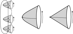
Figure 1: Left: Replicated $n$-manifold $(\mathcal{M}_{n},\mkern 1.5mu\overline{\mkern-1.5mug\mkern-1.5mu}\mkern 1.5mu_{\mathcal{A}})$ preparing fixed–area states. Center: Manifold $(\mathcal{M}_{n},\mkern 1.5mu\overline{\mkern-1.5mug\mkern-1.5mu}\mkern 1.5mu_{n})$ preparing Hartle–Hawking states. Right: The quotient geometry $(\mathcal{M}_{n}/\,\mathbb{Z}_{n},\mkern 1.5mu\overline{\mkern-1.5mug\mkern-1.5mu}\mkern 1.5mu_{n})$ for computation of HH entropy.

The entropy of each state is computed differently. First consider Hartle–Hawking states obeying boundary condition (5). Now assume the on-shell metric $\mkern 1.5mu\overline{\mkern-1.5mug\mkern-1.5mu}\mkern 1.5mu_{n}$ preserves replica symmetry [7], via $\tau\rightarrow\tau+2\pi k$ for integer $k\geq 1$. To perform the analytic continuation of $n$, it is useful to work with the orbifold $\mathcal{M}_{n}/\,\mathbb{Z}_{n}$, where now $\tau$ has identification $\tau\sim\tau+2\pi$. Equally, $\mathcal{M}_{n}/\,\mathbb{Z}_{n}=\mathcal{M}\,\backslash\,\mathcal{C}$ with $\tau\sim\tau+2\pi$ and $\mathcal{C}$ removed. Thence, $I_{\mathcal{M}_{n}}[\mkern 1.5mu\overline{\mkern-1.5mug\mkern-1.5mu}\mkern 1.5mu_{n}]=n\,I_{\mathcal{M}\,\backslash\,\mathcal{C}}[\mkern 1.5mu\overline{\mkern-1.5mug\mkern-1.5mu}\mkern 1.5mu_{n}]$, and the entropy (4) becomes

$$\widetilde{S}_{n}=n^{2}\partial_{n}\,I_{\mathcal{M}\,\backslash\,\mathcal{C}}[\mkern 1.5mu\overline{\mkern-1.5mug\mkern-1.5mu}\mkern 1.5mu_{n}],\quad(\text{HH state}).$$ (7)

As the integration region on $\mathcal{M}\,\backslash\,\mathcal{C}$ is independent of $n$, the $n$-derivative acts only on components of $\mkern 1.5mu\overline{\mkern-1.5mug\mkern-1.5mu}\mkern 1.5mu_{n}$, i.e., an on-shell variation of the action. This requires an analytic continuation of the on-shell action to non-integer $n$.

Alternatively, the solution $\mkern 1.5mu\overline{\mkern-1.5mug\mkern-1.5mu}\mkern 1.5mu_{\mathcal{A}}=\mkern 1.5mu\overline{\mkern-1.5mug\mkern-1.5mu}\mkern 1.5mu_{1}$ obeying the fixed-area condition (6) is independent of $n$ but depends on the area $\mathcal{A}$ of $\mathcal{C}$. Thus, the Rényi entropy (4) is

$$\widetilde{S}_{n}=(n\partial_{n}-1)\,I_{\mathcal{M}_{n}}[\mkern 1.5mu\overline{\mkern-1.5mug\mkern-1.5mu}\mkern 1.5mu_{\mathcal{A}}],\quad(\text{fixed-area state}),$$ (8)

with $\partial_{n}$ only acting on the integration region $\mathcal{M}_{n}$.

A distinction between the Rényi entropies of the Hartle–Hawking and fixed–area states is that the former is $n$-dependent while the latter is $n$-independent. Hence, the entanglement spectrum of a fixed–area state is ‘flat’ [22, 16]: the reduced density matrix describing the state is (approximately) proportional to the identity operator.

Entropy of Hartle–Hawking states. Let $g_{n}$ be an off-shell metric obeying (5) on $\mathcal{M}\,\backslash\,\mathcal{C}$ with $\tau\sim\tau+2\pi$. Notice that cutting $\mathcal{M}\,\backslash\,\mathcal{C}$ open along a codimension-1 surface $\mathcal{B}$, such that $\partial\mathcal{B}=\mathcal{C}$, produces a wedge shaped space $\mathcal{W}$ with two boundaries $\mathcal{B}_{\alpha}$ (with $\alpha=1,2$) meeting at a corner $\mathcal{C}=\mathcal{B}_{1}\cap\mathcal{B}_{2}$. See Fig. 2. Boundaries $\mathcal{B}_{1}$ and $\mathcal{B}_{2}$ are located at $\tau=0$ and $\tau=2\pi$, respectively. We emphasize, as a topological space, we treat $\mathcal{W}$ as an open set such that $\mathcal{B}_{\alpha}$ and $\mathcal{C}$ are not included in $\mathcal{W}$.

Notably, cutting has no effect on the value of the action as it only removes a sliver of measure zero from the integration region on $\mathcal{M}$. Thus,

$$I_{\mathcal{M}\,\backslash\,\mathcal{C}}[g_{n}]=I_{\mathcal{W}}[g_{n}].$$ (9)

The action of the wedge $\mathcal{W}$ is (in units $16\pi G_{\text{N}}=1$)

$$I_{\mathcal{W}}[g_{n}]=-\int_{\mathcal{W}}d^{D}x\sqrt{g_{n}}\,R-\sum_{\alpha=1}^{2}\int_{\mathcal{B}_{\alpha}}d^{D-1}x\sqrt{h_{\alpha}}\,2K_{\alpha}.$$ (10)

Here $h_{\alpha ij}$ is the induced metric on $\mathcal{B}_{\alpha}$, $K_{\alpha ij}=h_{\alpha i}^{k}h_{\alpha j}^{l}\nabla_{k}n_{\alpha l}$ is its extrinsic curvature with outward-pointing unit normal $n_{\alpha}^{a}$ to $\mathcal{B}_{\alpha}$. Despite $\mathcal{W}$ not including boundaries $\mathcal{B}_{\alpha}$, we have included a Gibbons–Hawking–York (GHY) term on each boundary. This is allowed to because the induced metrics and extrinsic curvatures of $\mathcal{B}_{\alpha}$ obey (the relative minus sign is due to oppositely pointing normals $n_{1,2}$),

$$h_{1ab}\lvert_{\mathcal{B}_{1}}\,=h_{2ab}\lvert_{\mathcal{B}_{2}},\quad K_{1ab}\lvert_{\mathcal{B}_{1}}\,=-K_{2ab}\lvert_{\mathcal{B}_{2}},$$ (11)

for integer $n\geq 1$ due to replica symmetry $\tau\sim\tau+2\pi k$ of $g_{n}$. Thus, the boundary terms cancel in (10) provided $n$ is an integer. For non-integer $n$, however, replica symmetry is broken, resulting in a discontinuity in the derivative of the metric when identifying the $\tau=0,2\pi$ surfaces. Thus, we work at integer $n$ and only analytically continue values of on-shell actions at the end.

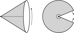
Figure 2: Cutting the manifold $(\mathcal{M}_{n}/\,\mathbb{Z}_{n},g_{n})$ into a wedge.

Varying the action (10) with respect to the metric without imposing any boundary conditions yields

$$\begin{split}&\delta_{g}I_{\mathcal{W}}=-\int_{\mathcal{W}}d^{D}x\sqrt{g}\,G_{ab}\,\delta g^{ab}+2\int_{\mathcal{C}}d^{D-2}x\sqrt{\sigma}\,\delta_{g}\Theta_{n}\\ &-\sum_{\alpha=1}^{2}\int_{\mathcal{B}_{\alpha}}d^{D-1}x\sqrt{h_{\alpha}}\,\widetilde{T}_{\alpha ab}\,\delta h^{ab}_{\alpha},\end{split}$$ (12)

where $G_{ab}$ is the Einstein tensor, $\widetilde{T}_{\alpha ab}=K_{\alpha ab}-K_{\alpha}h_{\alpha ab}$ is the boundary stress-tensor, and the corner angle is given by $\cos{\Theta_{n}}=g_{nab}\,n_{1}^{a}n_{2}^{b}$. Since the embedding of the first boundary is $\tau=0$ and the second is $\tau=2\pi$, explicitly we find $\Theta_{n}=\pi\,(1-2n^{-1})$.

Via the identity (9), we can obtain expressions for the action on the manifold $(\mathcal{M}\,\backslash\,\mathcal{C},g_{n})$ and its variation. Imposing periodic boundary conditions

$$\delta h_{1}^{ab}|_{\mathcal{B}_{1}}=\delta h_{2}^{ab}|_{\mathcal{B}_{2}},$$ (13)

such that the metric variation is continuous across the cut, the second line of variation (12) is cancelled when $n\geq 1$ is an integer. Since we want to extremize the action over metrics satisfying fixed-periodicity boundary condition (i) (5) at $\mathcal{C}$, the metric variation is such that $\delta n=0$. Thus, $\delta_{g}I_{\mathcal{M}\,\backslash\,\mathcal{C}}[g_{n}]=0$ imposes Einstein’s equations $G_{nab}=0$ on the metric $g_{n}$ everywhere outside $\mathcal{C}$.

Without going into detail (see [20, 15]), imposing Einstein’s equations provides a condition constraining $\mathcal{C}$. Namely, expanding the Ricci tensor near $\mathcal{C}$ yields

$$\mkern 1.5mu\overline{\mkern-1.5mu\sigma\mkern-1.5mu}\mkern 1.5mu_{1}^{ab}\,\mkern 1.5mu\overline{\mkern-1.5muL\mkern-1.5mu}\mkern 1.5mu_{\alpha ab}=\mkern 1.5mu\overline{\mkern-1.5mu\sigma\mkern-1.5mu}\mkern 1.5mu_{1}^{ab}\,\mkern 1.5mu\overline{\mkern-1.5muQ\mkern-1.5mu}\mkern 1.5mu_{\alpha ab}=0,$$ (14)

where $\mkern 1.5mu\overline{\mkern-1.5mu\sigma\mkern-1.5mu}\mkern 1.5mu_{1ab}$ is the induced metric and $\mkern 1.5mu\overline{\mkern-1.5muL\mkern-1.5mu}\mkern 1.5mu_{\alpha ab},\mkern 1.5mu\overline{\mkern-1.5muQ\mkern-1.5mu}\mkern 1.5mu_{\alpha ab}$ are extrinsic curvatures

$$L_{ab}=\sigma_{a}^{c}\,\sigma_{b}^{d}\,\nabla_{c}n_{\alpha d},\quad Q_{ab}=\sigma_{a}^{c}\,\sigma_{b}^{d}\,\nabla_{c}r_{\alpha d}.$$ (15)

of $\mathcal{C}$ in the solution $\mkern 1.5mu\overline{\mkern-1.5mug\mkern-1.5mu}\mkern 1.5mu_{1}$. Here $r_{\alpha}$ is a vector tangent to $\mathcal{B}_{\alpha}$ obeying $r_{\alpha}\cdot r_{\alpha}=1$ and $r_{\alpha}\cdot n_{\alpha}=0$. Thus, $\mathcal{C}$ is constrained to be a minimal area surface in $\mkern 1.5mu\overline{\mkern-1.5mug\mkern-1.5mu}\mkern 1.5mu_{1}$, and the variational principle for the HH metric fixes the embedding of $\mathcal{C}$.

Let us now determine the entropy functional. Working on-shell and using periodic boundary conditions (13),

$$\delta_{g}I_{\mathcal{M}\,\backslash\,\mathcal{C}}[\mkern 1.5mu\overline{\mkern-1.5mug\mkern-1.5mu}\mkern 1.5mu_{n}]=2\int_{\mathcal{C}}d^{D-2}x\sqrt{\mkern 1.5mu\overline{\mkern-1.5mu\sigma\mkern-1.5mu}\mkern 1.5mu_{n}}\,\delta_{g}\mkern 1.5mu\overline{\mkern-1.5mu\Theta\mkern-1.5mu}\mkern 1.5mu_{n},$$ (16)

where $n\geq 1$ is an integer to ensure cancellation of boundary terms via (11). To compute the entropy (7), however, we consider metric variations corresponding to $\delta n$, requiring analytic continuation of $n$ to real values. Extending to non-integer $n$, then using (16), the entropy (7) is

$$\widetilde{S}_{n}=2n^{2}\int_{\mathcal{C}}d^{D-2}x\sqrt{\mkern 1.5mu\overline{\mkern-1.5mu\sigma\mkern-1.5mu}\mkern 1.5mu_{n}}\,\partial_{n}\mkern 1.5mu\overline{\mkern-1.5mu\Theta\mkern-1.5mu}\mkern 1.5mu_{n}=4\pi\int_{\mathcal{C}}d^{D-2}x\sqrt{\mkern 1.5mu\overline{\mkern-1.5mu\sigma\mkern-1.5mu}\mkern 1.5mu_{n}}\;,$$ (17)

the area functional of the corner $\mathcal{C}$ in $\mkern 1.5mu\overline{\mkern-1.5mug\mkern-1.5mu}\mkern 1.5mu_{n}$. Further, the limit $n\to 1$ recovers prescription (1) with minimization determined by Einstein’s equations, (14), as in [7].

Entropy of fixed–area states. Consider an off-shell metric $g_{\mathcal{A}}$ obeying boundary condition (ii) (6). We cut the replicated manifold $(\mathcal{M}_{n},g_{\mathcal{A}})$ open, producing a manifold $(\mathcal{W}_{n},g_{\mathcal{A}})$ with boundaries $\mathcal{B}_{\alpha}$ (now at $\tau=0$ and $\tau=2\pi n$) meeting at a corner $\mathcal{C}$. The action satisfies

$$I_{\mathcal{M}_{n}}[g_{\mathcal{A}}]=I_{\mathcal{W}_{n}}[g_{\mathcal{A}}]+I_{\mathcal{C}}[g_{\mathcal{A}}],$$ (18)

where $I_{\mathcal{W}_{n}}$ is given by (10). We include a corner term to have a well-posed variational problem for fixed-area boundary conditions as $(\mathcal{W}_{n},g_{\mathcal{A}})$ has a corner in its interior (see below). It can be understood as the energy density supporting the conical excess present on $(\mathcal{M}_{n},g_{\mathcal{A}})$.

Unlike HH states, Einstein’s equations for $g_{\mathcal{A}}$ do not constrain the embedding of $\mathcal{C}$ for fixed-area states (see below). We thus derive fixed-area state entropy in three steps: (1) variational principle for the metric, (2) variational principle for the embedding of $\mathcal{C}$, and (3) show the entropy functional is the on-shell action of such solutions.

Variational principle for fixed–area metrics. The variational principle under area-preserving metric variations on the manifold $(\mathcal{M}_{n},g_{\mathcal{A}})$ is not well defined because of the angular excess at $\mathcal{C}$. Indeed, after the cutting procedure (18), the metric variation of the action includes a term localized at $\mathcal{C}$ which must be cancelled by the variation of $I_{\mathcal{C}}[g_{\mathcal{A}}]$ to make the variational problem well defined. This is achieved by the Hayward corner term [8]

$$I_{\mathcal{C}}[g_{\mathcal{A}}]=-2\int_{\mathcal{C}}d^{D-2}x\sqrt{\sigma}\,(\Theta_{1/n}+\pi).$$ (19)

Despite $g_{\mathcal{A}}$ being $n$-independent, the corner angle $\cos{\Theta_{1/n}}=g_{\mathcal{A}ab}\,n_{1}^{a}n_{2}^{b}$ is since the embedding of $\mathcal{B}_{2}$ depends on $n$; the two boundaries are at $\tau=0$ and $\tau=2\pi n$, giving $\Theta_{1/n}=\pi\,(1-2n)$. We have also included a corner “counterterm” proportional to $2\pi\mathcal{A}$ in (19), with a coefficient uniquely fixed such that the total corner term vanishes at $n=1$ (when there is no corner).

Equation (18) allows us to obtain the action of the replicated manifold $(\mathcal{M}_{n},g_{\mathcal{A}})$ from the wedge action (19). Via periodic boundary conditions, the codimension-1 boundary terms in (10) cancel for integer $n$, giving

$$I_{\mathcal{M}_{n}}[g_{\mathcal{A}}]=-n\int_{\mathcal{M}\,\backslash\,\mathcal{C}}d^{D}x\sqrt{g_{\mathcal{A}}}\,R-4\pi\,(1-n)\int_{\mathcal{C}}d^{D-2}x\sqrt{\sigma}\ .\hskip 2.84544pt$$ (20)

where we have used replica symmetry to pull out the factor of $n$ in the bulk integral. We have thus recovered the distributional contribution of a squashed conical excess to the Ricci scalar originally derived in [23]. There a regularization scheme was employed, including regularization dependent terms that enter at higher orders in $n-1\ll 1$ (except in two dimensions or when the extrinsic curvatures vanish). Notably, our corner method does not produce such terms.

We now extremize the action (20) over metrics with fixed area at $\mathcal{C}$. The variation of (20) follows from (18) and the variation of the wedge action (10) and the corner term (19). Under periodic boundary conditions we find

$$\begin{split}\delta_{g}I_{\mathcal{M}_{n}}=-\int_{\mathcal{M}_{n}}d^{D}x\sqrt{g_{\mathcal{A}}}\,G_{ab}\,\delta g^{ab}-\int_{\mathcal{C}}d^{D-2}x\sqrt{\sigma}\,\widehat{T}_{ab}\,\delta\sigma^{ab}\end{split}$$ (21)

with corner stress tensor $\widehat{T}_{ab}=-(\Theta_{1/n}+\pi)\,\sigma_{ab}$. The second term vanishes for area-preserving (traceless) variations $\delta\sigma^{ab}$ so that the variational principle imposes Einstein’s equations $G_{ab}=0$ on $g_{\mathcal{A}}$ everywhere on the replica manifold. So, the Hayward term, which was originally included to make the Dirichlet problem well defined, also makes the fixed-area variational problem well defined.

Extremization from variational problem of embedding. Einstein’s equations for $g_{\mathcal{A}}$ do not give constraints on the embedding of $\mathcal{C}$: since $n=1$ in (6), the Ricci tensor responsible for constraints (14) is zero. Thus, the variational problem for the embedding in the on-shell metric $\mkern 1.5mu\overline{\mkern-1.5mug\mkern-1.5mu}\mkern 1.5mu_{\mathcal{A}}$ is to be considered separately.

Recall $\mathcal{M}_{n}$ consists of $n$-copies of $\mathcal{M}$ cyclically glued together around $\mathcal{C}\subset\mathcal{M}$. Denote the embedding of $\mathcal{C}$ in $\mathcal{M}$ as $x^{a}=E^{a}(\hat{x})$ and define tangent vectors $e^{a}_{A}=\partial_{A}E^{a}$ that can be used to pull-back tensors to $\mathcal{C}$. Rather than directly varying the embedding, we keep the embedding fixed $\delta e^{a}_{A}=0$ and instead vary the background metric in the wedge $\mathcal{W}$ by an infinitesimal diffeomorphism

$$\delta_{\xi}g^{ab}=\nabla^{a}\xi^{b}+\nabla^{b}\xi^{a},\quad\xi^{a}=\xi^{n}n^{a}+\xi^{r}r^{a},$$ (22)

where we take the vector field $\xi$ to be normal to $\mathcal{C}$. We assume $\xi$ and its derivative are continuous across the cut so that the diffeomorphism descends to a transverse variation of the embedding of $\mathcal{C}$ in $\mathcal{M}_{n}$.

Under (22), the induced metric of $\mathcal{C}$ changes as [24]

$$\sigma_{c}^{a}\sigma_{d}^{b}\,\delta_{\xi}\sigma^{cd} =2\,\xi^{n}L^{ab}+2\,\xi^{r}Q^{ab}$$ (23)

for extrinsic curvatures of $\mathcal{C}$ in $\mkern 1.5mu\overline{\mkern-1.5mug\mkern-1.5mu}\mkern 1.5mu_{\mathcal{A}}$ (15). Applying the diffeomorphism (22) to the general variation (21) when the metric is on-shell $\mkern 1.5mu\overline{\mkern-1.5mug\mkern-1.5mu}\mkern 1.5mu_{\mathcal{A}}$ gives

$$\delta_{\xi}I_{\mathcal{M}_{n}}=-8\pi\,(1-n)\int_{\mathcal{C}}d^{D-2}x\sqrt{\sigma}\,(\xi^{n}\sigma_{ab}\,L^{ab}+\xi^{r}\sigma_{ab}\,Q^{ab}).$$ (24)

Requiring the variation to vanish gives the minimal surface condition (14) in $\mkern 1.5mu\overline{\mkern-1.5mug\mkern-1.5mu}\mkern 1.5mu_{\mathcal{A}}$, and is equivalent to the condition found by extremizing the area functional in $\mkern 1.5mu\overline{\mkern-1.5mug\mkern-1.5mu}\mkern 1.5mu_{\mathcal{A}}$ (cf. (26) below). Thus, the area extremization prescription for fixed-area states follows from varying the Einstein action via transverse diffeomorphisms of $\mathcal{C}$. This extremization coincides with the vanishing of the Hamiltonian charge generating $\xi$ [25].

Entropy functional. The above two variational principles determine the on-shell fixed-area metric $\mkern 1.5mu\overline{\mkern-1.5mug\mkern-1.5mu}\mkern 1.5mu_{\mathcal{A}}$ and the on-shell embedding of $\mathcal{C}$ in $\mathcal{M}$. Using (20) on-shell gives

$$I_{\mathcal{M}_{n}}[\mkern 1.5mu\overline{\mkern-1.5mug\mkern-1.5mu}\mkern 1.5mu_{\mathcal{A}}]=n\,I_{\mathcal{M}\,\backslash\,\mathcal{C}}[\mkern 1.5mu\overline{\mkern-1.5mug\mkern-1.5mu}\mkern 1.5mu_{\mathcal{A}}]-4\pi\,(1-n)\,\mathcal{A}.$$ (25)

where we used $\mkern 1.5mu\overline{\mkern-1.5mug\mkern-1.5mu}\mkern 1.5mu_{\mathcal{A}}=\mkern 1.5mu\overline{\mkern-1.5mug\mkern-1.5mu}\mkern 1.5mu_{1}$ respects replica symmetry. Consequently, the refined Rényi entropy (8) is

$$\widetilde{S}_{n}=4\pi\,\mathcal{A},$$ (26)

which is independent of $n$, corresponding to the flat entanglement spectrum of fixed-area states.

Discussion. Using Hayward corner terms, we developed a first principles prescription to compute gravitational Rényi entropy of Hartle–Hawking and fixed–area states in Einstein gravity. Via AdS/CFT duality, where the bulk is taken to be asymptotically AdS, our bulk computations directly translate to (refined) Rényi entropies of holographic CFTs. When $n\to 1$, we recover the Ryu–Takayanagi relation (1) for Hartle–Hawking states, and the analog for states of fixed–area/flat entanglement spectrum [14]. Previous work used the Hayward term to construct entropy functionals of fixed–area states [26], and Rényi entropy in Einstein and Jackiw–Teitelboim gravity [27, 28], but a complete consideration of variational problems for the metric and the corner embedding was lacking. Our formulation based on (9) and (18) allows for a careful treatment of the variational principle. Another appealing feature of our approach is that it readily extends to higher-curvature theories of gravity [15].

For example, for Lovelock gravity [29], which has a known corner term [30], the entropy functional of HH states is given by the Jacobson–Myers (JM) entropy [31], even when extrinsic curvatures are present. The variational principle of the wedge action is well-posed, giving Lovelock’s field equations, which provide a constraint for $\mathcal{C}$ coinciding with extremization of the JM functional. Moreover using the Lovelock corner term, fixed–area states generalize to fixed-JM states, where the Jacobson–-Myers functional of $\mathcal{C}$ is fixed. Thus, the entropy functional of a fixed-JM state is the Jacobson–-Myers functional with a flat spectrum. The extremization prescription arises from the variation of the Lovelock action of the wedge and coincides with the extremization of the JM functional. For arbitrary $F$(Riemann) gravity, corner terms are not known to exist assuming Dirichlet boundary conditions alone (this is also the case for GHY-like terms, cf. [32, 33, 34, 35, 36]). Hence, the variational problem in the presence of corners is not well-posed, and our method suggests fixed–area state analogs do not exist in such theories. For HH states, under special periodic boundary conditions, we can recover the Dong–Lewkowycz entropy [37], though it has not been proven if this is equal to the Camps–Dong prescription [38, 39]. We explain this extension and its limitations in [15].

Lastly, our analysis has been at the classical level. It would be interesting to generalize our approach to include bulk quantum corrections, along the lines of [40, 37]. Moreover, it would be worth extending the corner method to the covariant setting [41], where both timelike and spacelike Hayward terms are needed. We leave these extensions for future work.

Acknowledgements. We are grateful to Pablo Bueno, Luca Ciambelli, Elena Cáceres, Xi Dong, and Alejandro Vilar López for useful correspondence. We thank Manus Visser for many fruitful discussions and initial collaboration. JK is supported by the Deutsche Forschungsgemeinschaft (DFG, German Research Foundation) under Germany’s Excellence Strategy through the Würzburg-Dresden Cluster of Excellence on Complexity and Topology in Quantum Matter - ct.qmat (EXC 2147, project-id 390858490), as well as through the German-Israeli Project Cooperation (DIP) grant ‘Holography and the Swampland’. JK thanks the Osk. Huttunen foundation and the Magnus Ehrnrooth foundation for support during earlier stages of this work. AS is supported by STFC consolidated grant ST/X000753/1 and was partially supported by the Simons Foundation via It from Qubit Collaboration and by EPSRC when this work was initiated. AS thanks the Isaac Newton Institute for Mathematical Sciences, Cambridge, for support and hospitality during the program Black holes: bridges between number theory and holographic quantum information (supported by EPSRC grant no EP/R014604/1) as this work was being completed.

References

- Ryu and Takayanagi [2006a] S. Ryu and T. Takayanagi, Phys. Rev. Lett. 96, 181602 (2006a), arXiv:hep-th/0603001 .
- Ryu and Takayanagi [2006b] S. Ryu and T. Takayanagi, JHEP 08, 045, arXiv:hep-th/0605073 .
- Bekenstein [1972] J. D. Bekenstein, Lett. Nuovo Cim. 4, 737 (1972).
- Bekenstein [1973] J. D. Bekenstein, Phys. Rev. D 7, 2333 (1973).
- Hawking [1975] S. W. Hawking, Commun. Math. Phys. 43, 199 (1975), [Erratum: Commun.Math.Phys. 46, 206 (1976)].
- Hawking [1976] S. W. Hawking, Phys. Rev. D 13, 191 (1976).
- Lewkowycz and Maldacena [2013] A. Lewkowycz and J. Maldacena, JHEP 08, 090, arXiv:1304.4926 [hep-th] .
- Hayward [1993] G. Hayward, Phys. Rev. D 47, 3275 (1993).
- Banados et al. [1994] M. Banados, C. Teitelboim, and J. Zanelli, Phys. Rev. Lett. 72, 957 (1994), arXiv:gr-qc/9309026 .
- Hawking et al. [1995] S. W. Hawking, G. T. Horowitz, and S. F. Ross, Phys. Rev. D 51, 4302 (1995), arXiv:gr-qc/9409013 .
- Teitelboim [1995] C. Teitelboim, Phys. Rev. D 51, 4315 (1995), [Erratum: Phys.Rev.D 52, 6201 (1995)], arXiv:hep-th/9410103 .
- Teitelboim [1994] C. Teitelboim, in Cornelius Lanczos International Centenary Conference (NCSU 93) (1994) arXiv:hep-th/9405199 .
- Gibbons and Hawking [1977] G. W. Gibbons and S. W. Hawking, Phys. Rev. D 15, 2752 (1977).
- Fursaev [2006] D. V. Fursaev, JHEP 09, 018, arXiv:hep-th/0606184 .
- Kastikainen and Svesko [2023] J. Kastikainen and A. Svesko, (2023), arXiv:2312.13357 [hep-th] .
- Dong et al. [2019] X. Dong, D. Harlow, and D. Marolf, JHEP 10, 240, arXiv:1811.05382 [hep-th] .
- Headrick [2010] M. Headrick, Phys. Rev. D 82, 126010 (2010), arXiv:1006.0047 [hep-th] .
- Miao and Guo [2015] R.-X. Miao and W.-z. Guo, JHEP 08, 031, arXiv:1411.5579 [hep-th] .
- Miao [2015] R.-X. Miao, JHEP 10, 049, arXiv:1503.05538 [hep-th] .
- Camps [2016] J. Camps, JHEP 09, 139, arXiv:1605.08588 [hep-th] .
- Note [1] A remark on notation. It is common practice to write on the left-hand side of Eq. (4). We prefer because we treat topologically as a punctured disc (integrals range over , the surface is removed). This is consistent with [38].
- Akers and Rath [2019] C. Akers and P. Rath, JHEP 05, 052, arXiv:1811.05171 [hep-th] .
- Fursaev et al. [2013] D. V. Fursaev, A. Patrushev, and S. N. Solodukhin, Phys. Rev. D 88, 044054 (2013), arXiv:1306.4000 [hep-th] .
- Bhattacharyya and Sharma [2014] A. Bhattacharyya and M. Sharma, JHEP 10, 130, arXiv:1405.3511 [hep-th] .
- Balasubramanian and Cummings [2023] V. Balasubramanian and C. Cummings, (2023), arXiv:2312.08434 [hep-th] .
- Takayanagi and Tamaoka [2020] T. Takayanagi and K. Tamaoka, JHEP 02, 167, arXiv:1912.01636 [hep-th] .
- Botta-Cantcheff et al. [2020] M. Botta-Cantcheff, P. J. Martinez, and J. F. Zarate, JHEP 07 (07), 227, arXiv:2005.11338 [hep-th] .
- Arias et al. [2022] R. Arias, M. Botta-Cantcheff, and P. J. Martinez, JHEP 04, 130, arXiv:2112.10799 [hep-th] .
- Lovelock [1971] D. Lovelock, J. Math. Phys. 12, 498 (1971).
- Cano [2018] P. A. Cano, Phys. Rev. D 97, 104048 (2018), arXiv:1803.00172 [gr-qc] .
- Jacobson and Myers [1993] T. Jacobson and R. C. Myers, Phys. Rev. Lett. 70, 3684 (1993), arXiv:hep-th/9305016 .
- Dyer and Hinterbichler [2009] E. Dyer and K. Hinterbichler, Phys. Rev. D 79, 024028 (2009), arXiv:0809.4033 [gr-qc] .
- Deruelle et al. [2010] N. Deruelle, M. Sasaki, Y. Sendouda, and D. Yamauchi, Prog. Theor. Phys. 123, 169 (2010), arXiv:0908.0679 [hep-th] .
- Guarnizo et al. [2010] A. Guarnizo, L. Castaneda, and J. M. Tejeiro, Gen. Rel. Grav. 42, 2713 (2010), arXiv:1002.0617 [gr-qc] .
- Teimouri et al. [2016] A. Teimouri, S. Talaganis, J. Edholm, and A. Mazumdar, JHEP 08, 144, arXiv:1606.01911 [gr-qc] .
- Liu et al. [2017] H.-S. Liu, H. Lu, and C. N. Pope, JHEP 09, 146, arXiv:1708.02329 [hep-th] .
- Dong and Lewkowycz [2018] X. Dong and A. Lewkowycz, JHEP 01, 081, arXiv:1705.08453 [hep-th] .
- Dong [2014] X. Dong, JHEP 01, 044, arXiv:1310.5713 [hep-th] .
- Camps [2014] J. Camps, JHEP 03, 070, arXiv:1310.6659 [hep-th] .
- Faulkner et al. [2013] T. Faulkner, A. Lewkowycz, and J. Maldacena, JHEP 11, 074, arXiv:1307.2892 [hep-th] .
- Hubeny et al. [2007] V. E. Hubeny, M. Rangamani, and T. Takayanagi, JHEP 07, 062, arXiv:0705.0016 [hep-th] .