Localization of overdamped bosonic modes and transport in strange metals

Abstract

A recent theory described strange metal behavior in a model of a Fermi surface coupled a two-dimensional quantum critical bosonic field with a spatially random Yukawa coupling. With the assumption of self-averaging randomness, similar to that in the Sachdev-Ye-Kitaev model, numerous observed properties of a strange metal were obtained for wide range of intermediate temperatures, including the linear-in-temperature resistivity. The Harris criterion implies that spatial fluctuations in the local position of the critical point must dominate at lower temperatures. For an $M$-component boson with $M\geq 2$, we use multiple graphics processing units (GPUs) to compute the real frequency spectrum of the boson propagator in a self-consistent mean-field treatment of the boson self-interactions, but an exact treatment of multiple realizations of the spatial randomness from the random boson mass. We find that Landau damping from the fermions leads to the emergence of the physics of the random transverse-field Ising model at low temperatures, as has been proposed by Hoyos, Kotabage, and Vojta. This regime is controlled by localized overdamped eigenmodes of the bosonic scalar field, also has a resistivity which is nearly linear-in-temperature, and extends into a ‘quantum critical phase’ away from the quantum critical point, as observed in several cuprates. For the $M=1$ Ising scalar, the mean-field treatment is not applicable, and so we use Hybrid Monte Carlo simulations running on multiple GPUs; we find a rounded transition and localization physics, with strange metal behavior in an extended region around the transition.

This manuscript was compiled on

arXiv:2312.06751

Strange metals are an unusual state of quantum matter invariably present above the critical temperature of correlated electron superconductors, including the cuprate high temperature superconductors (1). They are characterized by numerous properties which deviate from the Fermi liquid description of conventional metals: most prominent among these are the linear-in-temperature resistivity, and the $1/\omega$ tail in the optical conductivity (2), where $\omega$ is frequency.

A recent work (3) proposed a universal theory of strange metals by considering the influence of spatially random electron-electron interactions on the theory of quantum phase transitions in metals (4). The spatial randomness was treated in a self-averaging manner, similar to the methods employed in the solution of the infinite-range Sachdev-Ye-Kitaev (SYK) models (5). This universal theory was found to be a good description of observations in a widening fan of temperatures emerging from the zero temperature quantum critical point (QCP).

However, strange metal behavior is often observed over wider regions of the phase diagram, and can appear in an extended region at low temperatures ($T$) away from the $T=0$ QCP (6, 7). Bashan et al. (8) postulated a non-zero density of two-level systems which resonantly scatter electrons, and argued that they can led to the needed extended quantum critical phase at low $T$. Here, we show that the self-averaging assumed in the universal theory (3) breaks down at very low $T$, and there is eventually a crossover to a regime where the overdamped bosonic modes of the quantum critical theory spatially localize. These localized bosonic modes are the analog of the two-level systems of Bashan et al. (8), and lead to an extended low $T$ quantum critical phase with a nearly linear in $T$ resistivity. We emphasize that our localized, overdamped bosonic modes are not postulated degrees of freedom, but emerge naturally in the existing theory after the flow to strong disorder at low $T$ is accounted for. We also note earlier works (9, 10, 11, 12) in which localized bosonic modes played an important role in other metallic correlated electron systems.

Section 1 describes an effective theory for the bosonic modes alone, and we present numerical results on its properties for $M\geq 2$ boson flavors in Section 2. The derivation of the effective boson only theory from the original fermion-boson theory of Ref. (3) is presented in Section 3, along with a description of electrical transport. We treat the $M=1$ Ising scalar case separately using an alternative technique in Section 4.

1 Effective theory for overdamped bosonic modes

We begin by considering a spatially random version of the Hertz-Millis theory of metallic QCPs (13) for a $M$-component bosonic field $\phi_{ja}(\tau)$ with action $\mathcal{S}_{\phi}+\mathcal{S}_{\phi d}$:

$$\mathcal{S}_{\phi}= \int d\tau\Bigl{[}\frac{J}{2}\sum_{\langle ij\rangle}\sum_{a}\left(\phi_{ia}-\phi_{ja}\right)^{2}$$

$$\leavevmode\nobreak\ \leavevmode\nobreak\ \leavevmode\nobreak\ \leavevmode\nobreak\ \leavevmode\nobreak\ \leavevmode\nobreak\ \leavevmode\nobreak\ \leavevmode\nobreak\ \leavevmode\nobreak\ \leavevmode\nobreak\ \leavevmode\nobreak\ \leavevmode\nobreak\ \leavevmode\nobreak\ \leavevmode\nobreak\ +\sum_{j}\bigl{(}\frac{\lambda+\lambda^{\prime}_{j}}{2}\sum_{a}\phi_{ja}^{2}+\frac{u}{4M}\left(\sum_{a}\phi_{ja}^{2}\right)^{2}\bigr{)}\Bigr{]}$$

$$\mathcal{S}_{\phi d}= \frac{T}{2}\sum_{\Omega}\sum_{j}\sum_{a}\left(\gamma|\Omega|+\Omega^{2}/c^{2}\right)|\phi_{ja}(i\Omega)|^{2}\,,$$ (1)

in two spatial dimensions. Here $a=1\ldots M$, $j$ labels the sites of a square lattice, $\tau$ is imaginary time, and $\Omega$ is Matsubara frequency. The action $\mathcal{S}_{\phi}+\mathcal{S}_{\phi d}$ can obtained by integrating out the fermions from the universal theory of Patel et al. (3) (see Eq. [10]). All couplings in $\mathcal{S}_{\phi}+\mathcal{S}_{\phi d}$ would then be spatially random, but we have only retained the spatial randomness in the tuning parameter $\lambda$ because that is the most relevant form of disorder by the Harris criterion (3, 13)—we have included a spatially random $\lambda_{j}^{\prime}$, whose disorder averages obey

$$\overline{\lambda_{j}^{\prime}}=0\quad,\quad\overline{\lambda_{j}^{\prime}\lambda_{k}^{\prime}}=\delta_{jk}\lambda^{\prime 2}\,.$$ (2)

The coupling $\gamma>0$ in $\mathcal{S}_{\phi d}$ is the Landau damping induced by the fermions, and the repulsive self-interaction $u>0$ plays an important role in stabilizing the theory in regions where $\lambda_{j}$ is very negative.

The bosonic field $\phi$ can represent a symmetry-breaking order parameter (such as a spin density wave or Ising nematic order), or a fractionalized field (such as a hybridization boson in Fermi volume changing transitions (14, 15, 16)).

For the case of $M\geq 2$ the global O($M$) symmetry is continuous, and important results for the properties of $\mathcal{S}_{\phi}+\mathcal{S}_{\phi d}$ were obtained by Hoyos et al. (17, 18), building on earlier work (19, 20, 21). Assuming that the renormalization group flow of $\lambda_{j}^{\prime}$ (and also of a spatially random addition to $J$) was towards a broad distribution, Hoyos et al. reached the remarkable conclusion that the low temperature properties near the QCP $\lambda=\lambda_{c}$ were the same as that of the random transverse field Ising model for insulators without any fermion-induced Landau damping. This random Ising model was shown to be described by infinite randomness fixed points by Fisher (22, 23) in $d=1$ spatial dimension; numerical studies in $d=2$ (24, 25) also support infinite randomness fixed points. The argument of Hoyos et al. relies on the fact that the $|\Omega|$ Landau damping term in $\mathcal{S}_{\phi d}$ is equivalent to a long-range $\phi$-$\phi$ interaction which decays as $1/\tau^{2}$ in imaginary time. Then the quantum dynamics of a droplet which is nearly ordered can be mapped on to the statistical mechanics of a one-dimensional chain of O($M$) spins with an inverse-square interaction; this classical model has no phase transition, but a correlation length which diverges exponentially with the inverse classical ‘temperature’ (26). This exponentially large correlation length is similar to the exponentially large correlation length of classical Ising chains with short-range interactions (27), and hence the mapping of Hoyos et al.. This mapping can be understood as a compensation between the enhancement of local quantum fluctuations in a droplet by the continuous symmetry, and the suppression of quantum fluctuations by the fermion-induced dissipation, leading to a mapping to a non-dissipative quantum system with a discrete symmetry. For the case of $M=1$, the ordered droplets have no additional fluctuations, leading to the destruction of the Griffiths phase and a smearing of the QCP (28, 29).

2 Numerical results for the bosonic theory

We have obtained numerical results for the properties of $\mathcal{S}_{\phi}+\mathcal{S}_{\phi d}$. When $M\geq 2$, we follow the analysis of Del Maestro et al. (30) for the same theory in a different context in $d=1$. We solve the large $M$ saddle-point equations in a finite sample exactly in the presence of specific realizations of disorder. Modern computing hardware makes such a numerical solution possible for large systems in $d=2$, as we will describe below. The large $M$ method makes it possible to perform exact analytic continuation to real time, and that will be important for our computation of the fermion spectrum and transport properties. Moreover, we expect the large $M$ method to accurately capture the physics of the infinite disorder physics because the exponential divergence of the droplet correlation time is also present in the classical limit. We note that the numerical large $M$ solutions in $d=1$ were in excellent agreement (30) with exact theoretical predictions for the critical properties (22, 23).

The large $M$ saddle point equations amount to replacing $\mathcal{S}_{\phi}$ by

$$\overline{\mathcal{S}}_{\phi}= \int d\tau\Bigl{[}\frac{J}{2}\sum_{\langle ij\rangle}\left(\phi_{ia}-\phi_{ja}\right)^{2}+\sum_{j}\frac{\overline{\lambda}^{\prime}_{j}}{2}\phi_{ja}^{2}\Bigr{]}$$ (3)

$$\overline{\lambda}^{\prime}_{j}=\lambda+\lambda^{\prime}_{j}+\frac{u}{M}\sum_{a}\left\langle\phi_{ja}^{2}\right\rangle_{\overline{\mathcal{S}}_{\phi}+\mathcal{S}_{\phi d}}$$ (4)

The numerical solution of this equation involves diagonalization of the boson propagator implied by $\overline{\mathcal{S}}_{\phi}$. At a given $\lambda$, we then compute self-consistent renormalized ‘mass’ $\overline{\lambda}_{j}$ by updating it iteratively using Eq. [4].

We used $J=1,\leavevmode\nobreak\ \gamma=1,\leavevmode\nobreak\ c^{2}=10$, and $u=1$ throughout this work, with the variance of the random mass, i.e. ${\lambda^{\prime}}^{2}$, taken to be $0.25$. The size of the $L\times L$ systems was set to $L=160$ unless otherwise mentioned, with periodic boundary conditions. The main challenge in obtaining a numerical solution of Eq. [4] is that the eigenvalues of the self-consistent boson propagator must be positive, or else the solution is unphysical. We therefore started from a value of $\lambda$ far from criticality in the disordered phase, which allowed for a positive definite self-consistent boson propagator, and then pushed $\lambda$ towards criticality using solutions at previous values of $\lambda$ as initial conditions.

The allowed $\lambda$ step size to retain positive-definiteness of the boson propagator became progressively smaller as the critical point was approached. Therefore, getting data in the critical regime for the parameter values we analyzed required up to order 10,000 matrix diagonalizations of 25,600$\times$25,600 matrices per disorder realization, as well as the same number of frequency summations over up to order 10,000 Matsubara frequencies per eigenvalue of the matrices and per disorder realization. We executed these operations in a massively parallel manner on a graphics processing unit (GPU), and also utilized multiple GPUs to execute multiple disorder realizations in parallel for high throughput. The use of GPUs reduced matrix diagonalization times down from tens of minutes to just a few seconds, and frequency summation times from tens of seconds to just milliseconds, which made solving the problem possible on a reasonable timescale.

We computed the boson correlator

$$D_{ij}(i\Omega)=\frac{1}{M}\left\langle\phi_{ia}(i\Omega)\phi_{ja}(-\Omega)\right\rangle=\sum_{\alpha}\frac{\psi_{\alpha i}\psi_{\alpha j}}{\gamma|\Omega|+\Omega^{2}/c^{2}+e_{\alpha}}\,$$ (5)

where $e_{\alpha}$ and $\psi_{\alpha j}$ are eigenvalues and eigenfunctions of the $\phi$ quadratic form in $\overline{\mathcal{S}}_{\phi}$, labeled by the index $\alpha=1\ldots L^{2}$ for a $L\times L$ sample. We also computed the spatial Fourier transform

$$D({\bm{q}}_{1},{\bm{q}}_{2},i\Omega)=\frac{1}{L^{4}}\sum_{i,j}D_{ij}(i\Omega)e^{i{\bm{q}}_{1}\cdot{\bm{r}}_{i}-i{\bm{q}}_{2}\cdot{\bm{r}}_{j}}\,.$$ (6)

where ${\bm{r}}_{j}$ is spatial co-ordinate of site $j$, and ${\bm{q}}_{1,2}$ are two-dimensional momenta.

From fitting the decay of the spatially averaged $D_{ij}(i\Omega)$ at large $|{\bm{r}}_{i}-{\bm{r}}_{j}|$ to $e^{-|{\bm{r}}_{i}-{\bm{r}}_{j}|/\xi}$, we obtained the correlation length $\xi$, shown in Fig 1.

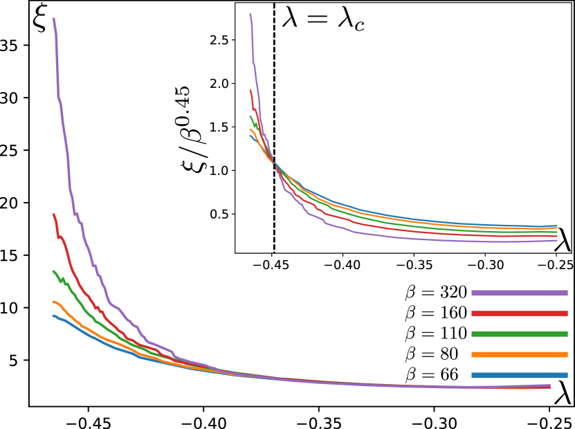
Figure 1: Correlation length as a function of the tuning parameter $\lambda$, for different values of $\beta=1/T$. (inset) The crossing point where $\xi$ scales as a power law in $\beta$ ($\xi\sim\beta^{0.45}$) estimates the position of the critical point $\lambda_{c}\approx-0.447$. There is long-range order in $\phi$ for $\lambda<\lambda_{c}$ at $T=0$.

A strong $T$ dependence of $\xi$ appears only for smaller values of $\lambda$, and from this we identify the position of the $T=0$ QCP $\lambda=\lambda_{c}$ as the point where the correlation length can be best described to be a power law in the inverse temperature $\beta$, i.e. $\xi\sim\beta^{m}$. There is long-range order in $\phi$ for $\lambda<\lambda_{c}$ at $T=0$.

We examine the frequency and momentum dependencies of $D^{-1}({\bm{q}},{\bm{q}},i\Omega)$ at the QCP $\lambda=\lambda_{c}$ in Fig 2. We find a $|\Omega|$ frequency dependence and a $q^{2}$ momentum dependence at all non-zero Matsubara frequencies (Fig. 2a,b), as expected from the averaged theory (3). However, at $\Omega=0$ we find a noisy momentum dependence that is strongly sensitive to the chosen disorder sample, indicating the influence of localized modes at low energies (Fig. 2b). This is confirmed by an examination of $D({\bm{q}}_{1},{\bm{q}}_{2},i\Omega)$ with unequal ${\bm{q}}_{1,2}$: while the $\Omega\neq 0$ results are strongly peaked at ${\bm{q}}_{1}={\bm{q}}$, the $\Omega=0$ results have large off-diagonal components (Fig. 2c). The frequency dependence also shows a downturn at the zeroth Matsubara frequency, which indicates a change of physics from that of the averaged theory at low energies (Fig. 2a).

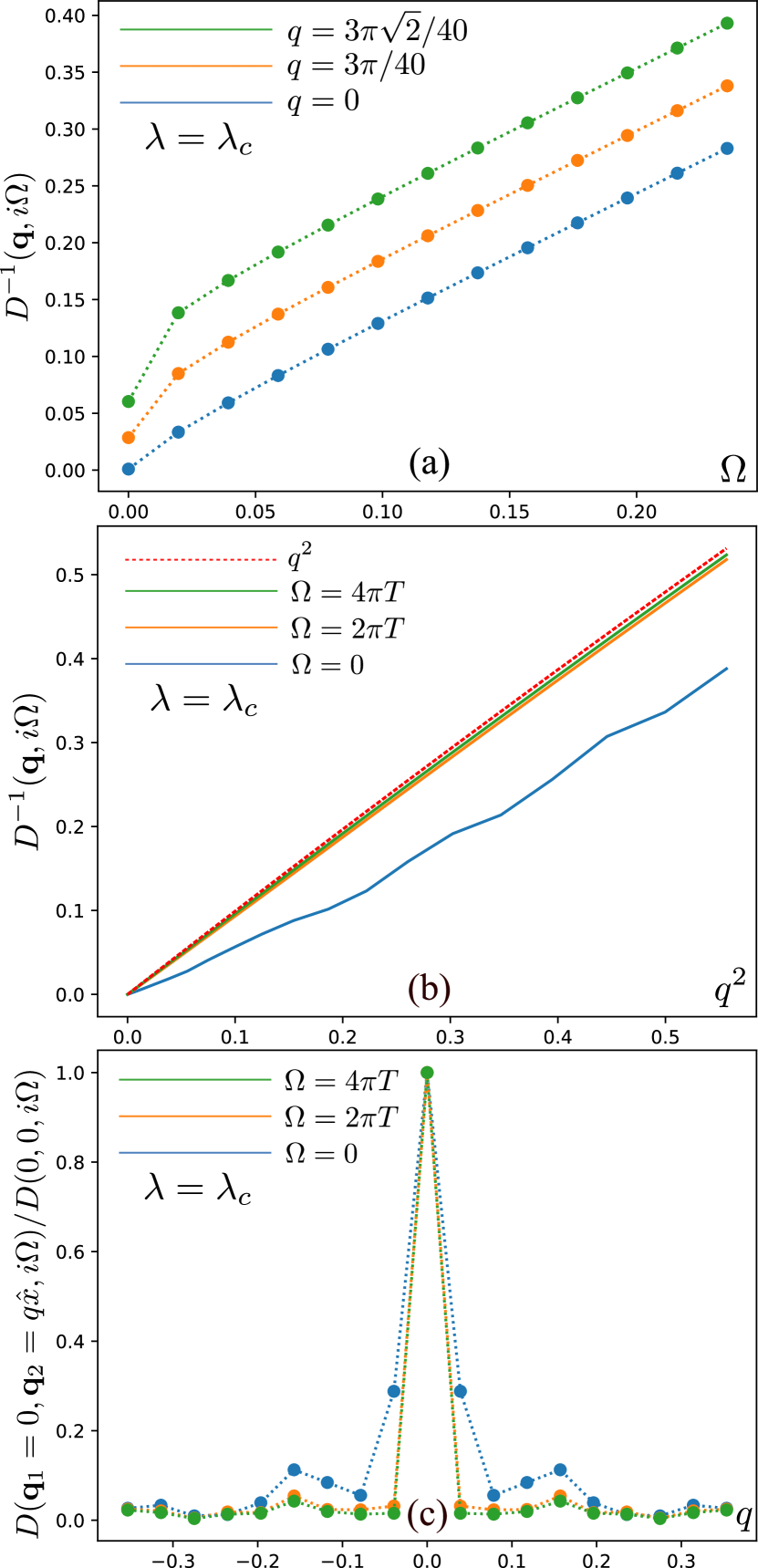
Figure 2: (a) Frequency dependence of $D({\bm{q}},i\Omega)\equiv D({\bm{q}},{\bm{q}},i\Omega)$ at the quantum critical coupling $\lambda=\lambda_{c}$. Results for other values of $\lambda$ appear in SI Appendix Fig. LABEL:fig:boson_prop_w_supp. (b) Momentum dependence of $D({\bm{q}},i\Omega)$ for different Matsubara frequencies, at the quantum critical coupling $\lambda=\lambda_{c}$. Results for other values of $\lambda$ appear in SI Appendix Fig. LABEL:fig:boson_prop_supp. (c) Momentum off-diagonal components of $D({\bm{q}}_{1}=0,{\bm{q}}_{2},i\Omega)$ for different Matsubara frequencies, again at $\lambda=\lambda_{c}$. The zeroth Matsubara frequency shows a significant off-diagonal component. These results were obtained for a single disorder sample at $\beta=320$.

A more explicit demonstration of the localization of the low energy modes is presented in Fig. 3.

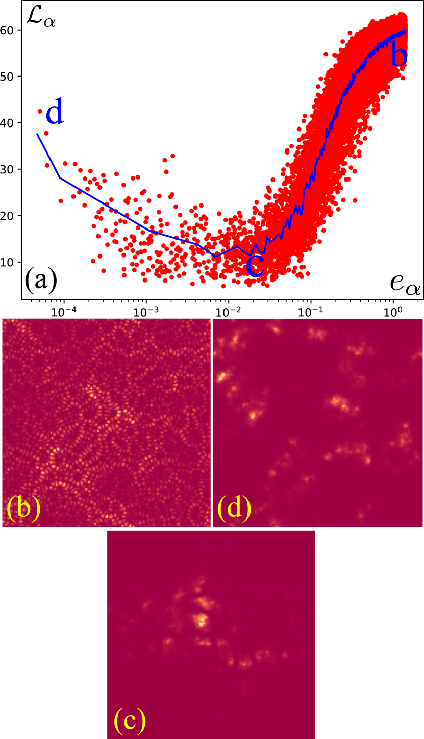
Figure 3: (a) Localization lengths $\mathcal{L}_{\alpha}$ of the overdamped bosonic modes in a collection of 10 disorder samples as a function of the eigenvalue $e_{\alpha}$ of the inverse bosonic propagator, at $\lambda=\lambda_{c}$ and $\beta=800$. The blue curve denotes the average localization length across samples in a given eigenvalue bin. Results for other values of $\lambda$ appear in SI Appendix Fig. LABEL:fig:loc_length_supp. (b, c, d) Plot of the bosonic eigenstates, $\psi_{\alpha j}$ as a function of ${\bm{r}}_{j}$. The corresponding eigenvalue is noted in (a). The delocalized states with higher $e_{\alpha}$ are superpositions of plane waves, as is apparent from the interference patterns in (b). These transition into strongly localized lower energy states in (c), and start to delocalize again at very low energies in (d). However, the delocalized states in (d) are not wave-like and break translational invariance strongly, as evidenced by the lack of interference patterns.

We compute the localization length by determining the localization volume to be equal to the reciprocal of the inverse participation ratio ($\mathcal{I}_{\alpha}$) of the normalized low energy eigenvectors $\psi_{\alpha}$ of $D^{-1}$; the localization length ($\mathcal{L}_{\alpha}$) is then obtained from the localization volume by assuming an isotropic exponential decay of the eigenvectors:

$$\mathcal{I_{\alpha}}\equiv\sum_{j}\psi_{\alpha j}^{4},\leavevmode\nobreak\ \leavevmode\nobreak\ \mathcal{L_{\alpha}}\equiv\frac{1}{\sqrt{2\mathcal{I_{\alpha}}}}.$$ (7)

The higher energy modes have a localization length of $\mathcal{O}(L/2)$, as is expected for fully delocalized states in a system with periodic boundary conditions. We expect the universal SYK-type theory of Patel et al. (3) to apply at such energies. But at lower energies, Fig. 3a shows a minimum of the localization length, and a slow subsequent increase of the localization length at the lowest energies. This non-monotonic behavior, and the lowest energy increase of the localization length, is just as expected from the physics of the random transverse field Ising model. In the real-space Dasgupta-Ma renormalization group procedure (31), higher energy localized modes renormalized the couplings of lower energy modes at lower energy, leading to the activated dynamic scaling of the localization length with damping rate $e_{\alpha}$ (22, 23, 24)

$$\mathcal{L}_{\alpha}\sim\left[\ln(1/e_{\alpha})\right]^{\mu}\,,$$ (8)

where $\mu$ is an exponent. This logarithmic dependence of length scale on energy is consistent with slow increase of the localization length in Fig. 3a at the lowest energy.

We also show a plot of the averaged density of states of eigenmodes of the boson propagator

$$\rho(\omega)=\overline{\delta(\omega-e_{\alpha})}$$ (9)

in Fig. 4.

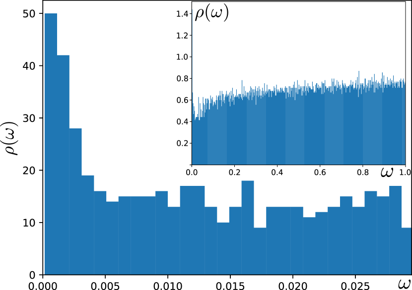
Figure 4: Density of states of boson eigenmodes $\rho(\omega)$ averaged over 10 disorder samples. A larger $\omega$ range is shown in the inset. The localized boson eigenmodes lead to an increase in $\rho(\omega)$ at the lowest energies. These results were obtained at $\beta=320$ and $\lambda=\lambda_{c}$.

The density of states is roughly constant for most of the energy range, as is expected for a $q^{2}$ boson dispersion in $d=2$, but increases as $\omega\rightarrow 0$, where the localized lowest-energy eigenvectors are clustered.

3 Fermion and transport properties

We now turn to the full model which includes fermionic degrees of freedom. The model underlying $\mathcal{S}_{\phi}+\mathcal{S}_{\phi d}$ in Eq. [1] is that examined by Patel et al. (3), and involves electrons $c_{i}$ (we do not write out the electron spin components) coupled to the bosonic modes with imaginary time action

$$\mathcal{S}= \mathcal{S}_{\phi}+\mathcal{S}_{c}+\mathcal{S}_{Y}$$

$$\mathcal{S}_{c}= \int d\tau\sum_{{\bm{k}}}c_{{\bm{k}}}^{\dagger}\left(\frac{\partial}{\partial\tau}+\varepsilon_{{\bm{k}}}\right)c_{{\bm{k}}}$$

$$\mathcal{S}_{Y}= \int d\tau\sum_{j}(g+g^{\prime}_{j})\,\phi_{ja}c_{j}^{\dagger}\sigma^{a}_{j}c_{j}\,.$$ (10)

Here ${\bm{k}}$ is a two-dimensional momentum, $\varepsilon_{\bm{k}}$ is the electron dispersion with a simple convex Fermi surface, $\sigma^{a}_{j}$ is a fixed coupling matrix depending upon the nature of the field $\phi$, and the Yukawa coupling $g+g_{j}^{\prime}$ has a spatially random component obeying

$$\overline{g_{j}^{\prime}}=0\quad,\quad\overline{g_{j}^{\prime}g_{k}^{\prime}}=\delta_{jk}g^{\prime 2}\,.$$ (11)

Patel et al. (3) argued that the spatial randomness in $\lambda+\lambda_{j}^{\prime}$ could be ‘gauged away’ by rescaling $\phi_{j}$, and then analyzed $\mathcal{S}$ with a spatially independent $\lambda$, averaging over the disorder $g_{j}^{\prime}$ along the lines of the Yukawa-SYK model (32, 33). We expect that this procedure should be applicable as long as we are in the regime with extended bosonic eigenmodes, above the minimum in Fig. 3a. But we do not expect it to be applicable in the strong disorder regime associated with the localized bosonic eigenmodes below the minimum in Fig. 3a.

Here, we wish to describe the consequences of the crossover in the bosonic eigenmodes in Fig. 3 in the electronic spectrum. To this end, we will use the bosonic eigenmodes of Section 2 to compute the electron self energy perturbatively in $g+g_{j}^{\prime}$, assuming that the electronic eigenmodes remain extended. For the extended bosonic eigenmodes, it has been argued (3) that the fermion self energy due to the spatially uniform coupling $g$ cancels in the computation of transport properties. For the localized bosonic modes, the influence of $g$ and $g_{j}^{\prime}$ in the electronic self energy should be similar, as the randomness in the eigenfunctions $\psi_{\alpha j}$ ensures lack of momentum conservation. So for transport properties, it is adequate to follow the simpler procedure of computing the electronic self energy only from $g_{j}^{\prime}$, and using the imaginary part of the retarded self energy as a proxy for the transport scattering rate. We therefore compute the average perturbative electronic self energy via

$$\Sigma(i\omega) =-i\pi g^{\prime 2}\mathcal{N}_{0}\frac{T}{L^{2}}\sum_{j,\Omega}\mbox{sgn}(\omega+\Omega)D_{jj}(i\Omega)$$

$$=-i\pi g^{\prime 2}\mathcal{N}_{0}\frac{T}{L^{2}}\sum_{\alpha,\Omega}\frac{\mbox{sgn}(\omega+\Omega)}{\gamma|\Omega|+\Omega^{2}/c^{2}+e_{\alpha}},$$ (12)

where $\mathcal{N}_{0}$ is the density of electronic states at the Fermi level, associated with the dispersion $\varepsilon_{\bm{k}}$. The last expression is only valid for the large $M$ self-consistent approach, and now the Matsubara summation can be performed exactly in closed form (see SI Appendix Eq. [LABEL:analytical_self_en]), with the sum over eigenvalues $e_{\alpha}$ subsequently performed numerically. Therefore, an important advantage of this computational procedure is that we can perform an exact analytic continuation to real frequencies, $i\omega\rightarrow\omega+i0^{+}$, and then obtain the retarded fermion self energy $\Sigma^{R}(\omega)$ on the real frequency axis. Taking the imaginary part of $\Sigma^{R}(\omega)$, we obtain the results for the $\omega$ dependence of the transport scattering rate shown in Fig. 5. We find a power-law dependence on $\omega$ for $\omega\gg T$. The exponent $n$ of the power law is approximately $1$ for a range of $\lambda>\lambda_{c}$, indicating the extension of the strange metal (which is defined by an exponent $n=1$ in the transport scattering rate) into a ‘quantum critical phase’ away from the QCP.

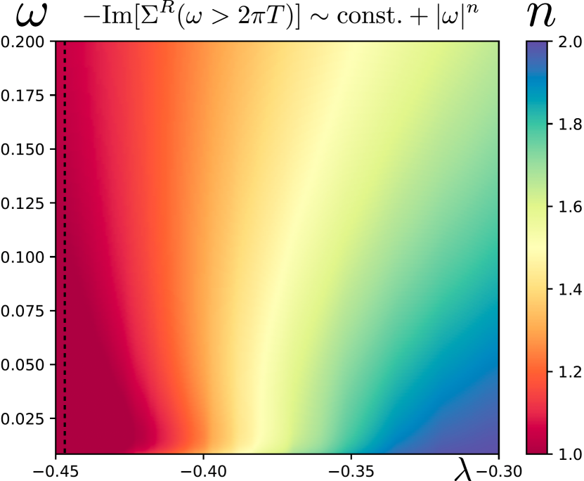
Figure 5: Power-law scaling in the frequency ($\omega\gg T$) dependence of the transport scattering rate inferred from the contribution to the single particle self energy from spatially random ($g^{\prime}$) interactions. The dashed line represents $\lambda=\lambda_{c}$. These results were obtained at $\beta=800$ and are an average over $10$ disorder samples. An exponent $n\sim 1$ is seen over an extended region away from the QCP that becomes wider in $\lambda$ at lower energy scales, thereby resembling the results of Ref. (6). The exponent $n$ is determined using $n=-d\ln(\mathrm{Im}[\Sigma^{R}(\omega)]-\mathrm{Im}[\Sigma^{R}(0)])/d\ln\omega$.

Finally, we compute the DC resistivity $\rho_{\mathrm{DC}}$ from $\mathrm{Im}[\Sigma^{R}(\omega)]$, using the standard relation (34) that is valid for transport determined by the non-momentum conserving scattering arising from the spatially random part $g^{\prime}$ of the Yukawa coupling:

$$\frac{1}{\rho_{\mathrm{DC}}(T)}=\frac{\pi v_{F}^{2}\mathcal{N}_{0}}{8T}\int_{-\infty}^{\infty}\frac{d\omega}{2\pi}\mathrm{sech}^{2}\left(\frac{\omega}{2T}\right)\frac{1}{\mathrm{Im}[\Sigma^{R}(\omega)]},$$ (13)

where $v_{F}$ is the average Fermi velocity of the electrons. We plot the $T$-dependence of the DC resistivity in Fig. 6. A linear temperature dependence of the resistivity is seen for a significant range of $\lambda>\lambda_{c}$, again indicating a ‘quantum critical phase’. Eventually, for $\lambda\gg\lambda_{c}$, the temperature dependence crosses over to the quadratic scaling expected in a Fermi liquid. Interestingly, we also observe a finite residual resistivity, that becomes significant as $\lambda\rightarrow\lambda_{c}$. Its origin can be traced back to the large boson density of states at $\omega\rightarrow 0$ shown in Fig. 4. From Eq. [12], a cluster of near-zero eigenvalues $e_{\alpha}$ can be seen to produce a nearly $\omega$-independent offset in $\Sigma(i\omega)$ and $\mathrm{Im}[\Sigma^{R}(\omega)]$, which translates into a residual resistivity through Eq. 13. The physical interpretation of this effect is simple - the lowest energy boson eigenstates are localized in nature and are also nearly frozen with very slow dynamics, and therefore simply act as local elastic impurity scatterers of the electrons, giving rise to a residual resistivity.

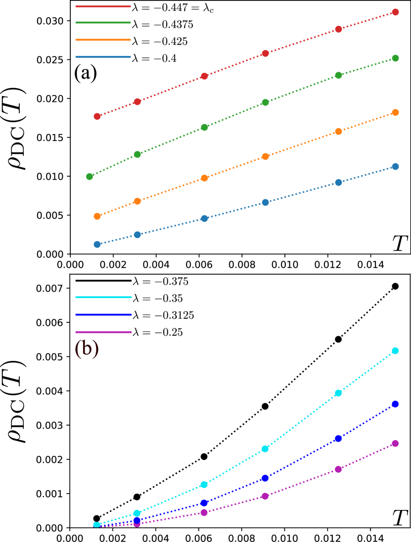
Figure 6: (a) DC resistivity $\rho_{\mathrm{DC}}(T)$ vs temperature $T$. A roughly linear dependence on $T$ is seen over an extended region away from the QCP, along with a residual resistivity, thereby resembling the results of Ref. (6). (b) DC resistivity further away from the QCP, showing superlinear scaling in $T$, and eventually transitioning into the Fermi-liquid $T^{2}$ scaling far away from the QCP. These results were obtained by averaging over 10 disorder samples.

4 $M=1$ Ising scalar

When $M=1$, the large $M$ saddle point Eqs. (4) are no longer applicable. We therefore simulate the theory of Eq. (1) using a Hybrid Monte Carlo (HMC) algorithm. We use a HMC method recently developed for critical fermionic theories (35), but without the fermions, running on multiple GPUs to sample over many disorder configurations. We find that the sharp QCP becomes smeared over some region of $\lambda$, as indicated by the correlation length and the susceptibility and shown in Fig. 7.

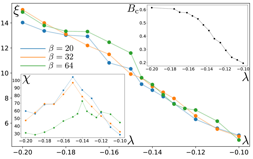
Figure 7: Observables describing the rounded phase transition for the $M=1$ Ising scalar. The main figure shows the correlation length of the equal-time propagator, $\xi$, plotted as a function of $\lambda$, for an $L=80$ system and with $40$ disorder configurations. Unlike the $M\geq 2$ case, $\xi$ does not diverge (or even change) with temperature in the entire critical region, indicating the absence of a sharp transition. The inset in the upper right corner shows the Binder cumulant, $B_{c}=1-\overline{\langle\Phi^{4}\rangle/(3\langle\Phi^{2}\rangle^{2})}$, where $\Phi\equiv\phi(\Omega=0,\bm{q}=0)$, plotted as a function of $\lambda$, for $L=64,\beta=32$ and with $120$ disorder configurations. The shape of the curve tells us the approximate ‘smeared critical’ region, as well as the $\lambda$ beyond which $B_{c}$ is close to the limiting value of $0.66$ and can be considered ‘ordered’. We plot only one value of $\beta,L$ as no crossing point will occur in this case. The inset in the lower left corner shows the uniform static susceptibility $\chi$. All curves are for $L=80$, and the $\beta=20,32$ ($\beta=64$) curves use $100-200$ ($40$) disorder configurations. As expected, the susceptibility peak does not become sharper with lower $T$, as is the case for QCPs. However, the presence of a peak indicates a smaller region of $\lambda$ where we expect the most critical-like behavior.

This is consistent with the predictions of Refs. (28, 29). In this ‘smeared critical’ region, the disorder variance is significantly enhanced compared to the $M\geq 2$ case, with hundreds of disorder configurations required to smooth out many of the observables for which only a few configurations were sufficient at large $M$. The wavefunction localization lengths $\mathcal{L}_{\alpha}$ are shown in SI Appendix Fig. LABEL:fig:LLs_supp and behave largely the same as in Fig. 3a, but with a few differences: there are significantly fewer localized eigenmodes, and the de-localized but translation-symmetry breaking lowest eigenmodes get spectrally separated from the localized ones as $\lambda$ is lowered. The former is again consistent with the absence of a Griffiths phase where a large density of localized eigenmodes give a critical spectral density at low energies. The latter is a novel observation, and we attribute these states to ordered puddles which are no longer fluctuating do to the discrete symmetry breaking. More plots of bosonic properties are shown in the SI Appendix.

Although the HMC solution does not enable us to analytically continue the fermion self-energy, we can still evaluate it on the Matsubara axis using the first expression of Eq. [12]. In the entire ‘smeared critical’ region, we observe a very distinct marginal Fermi-liquid (MFL) scaling of $\mathrm{Im}[\Sigma(i\omega)]$, as shown in Fig. 8.

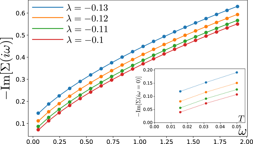
Figure 8: The fermion self-energy $-\mathrm{Im}[\Sigma(i\omega)]$ as a function of Matsubara frequency $\omega$, in the ‘smeared critical’ region for $M=1$. All curves are for an $L=80$ system at $\beta=64$, using an average over $100$-$200$ disorder realizations. The lines are fits to the MFL form $a\,\omega\log(b/|\omega|)+c$, which has a UV cutoff $b$ and a $\omega=0$ scattering rate $c$. The MFL form is very well fit for all $\lambda$ values shown, with coefficients for all curves in the ranges: $0.083<a<0.088$, $41<b<46$, and $0.04<c<0.12$ (increasing with decreasing $\lambda$). (inset) The extrapolated value of $-\mathrm{Im}[\Sigma(i\omega=0)]$ from the MFL fit vs temperature $T$, showing a $T$ dependence of roughly $-T\ln T$ along with a residual scattering rate, as expected for a MFL.

Based on the arguments of Patel et al. (3) and those in the previous section, upon analytic continuation to real frequencies this MFL self energy is what leads to strange metal behavior with linear-in-temperature and linear-in-frequency transport scattering rates.

5 Discussion

The recent universal theory of strange metals by Patel et al. (3) considered the action $\mathcal{S}$ in Eq. [10] of electrons $c_{j}$ coupled to quantum critical bosonic scalars $\phi_{ja}$. They argued that the random ‘mass’ spatial disorder $\lambda_{j}^{\prime}$ in Eq. [1] could be absorbed by a rescaling of the scalar fields $\phi_{ja}$, resulting in an enhancement of the spatial disorder in the Yukawa coupling $g_{j}^{\prime}$ in Eq. [10]. They performed a self-consistent and self-averaging analysis of the resulting action, similar to that required for the exact solution of the SYK model (5). This theory matched numerous observations in strange metals, including the $T$-linear resistivity, the Planckian relaxation time, the $T\ln(1/T)$ specific heat, and the $1/\omega$ optical conductivity.

The present paper has focused closer attention on the role of the random mass spatial disorder $\lambda_{j}^{\prime}$. We have shown that the rescaling procedure of Patel et al. (3) remains valid in an intermediate temperature regime where the eigenmodes of the zero frequency boson propagator remain extended. However, new physics emerges at low temperatures when the boson eigenmodes localize, resulting in an extended regime of strange metal behavior away from the QCP. This extended regime is proposed as an explanation of observations by Cooper et al. (6) and Greene et al. (7).

Our key results for the localization of the boson eigenmodes for $M\geq 2$ appear in Fig. 3. At higher energies, the bosonic eigenmodes are extended, as in Fig. 3b. The extended bosonic eigenmodes have a density of states which is independent of energy, as shown in Fig. 4, and as found in the SYK-type analysis by Patel et al. (3). This constant density of states results in a linear-in-$T$ resistivity (Fig. 6), that we found to extend away from QCP. Fig. 3a shows a minimum in the localization length below which the localization length shows a logarithmically slow increase with decreasing energy. We have argued that this low energy regime is described (17, 18) by the strong-disorder Griffiths regime of the random transverse field Ising model (22, 23). We computed the effect of these localized eigenmodes on electronic transport perturbatively, and showed that they produce a significant contribution the residual resistivity as the QCP is approached. However, it would be worthwhile to examine the contributions of the localized modes more completely in future work.

For the case of the $M=1$ Ising scalar, the localized modes are far fewer in number, which leads to an absence of a Griffiths phase and a ‘smeared critical’ region which replaces the sharp QCP of $M\geq 2$. Like in the $M\geq 2$ case, this region also shows strange metal behavior at finite energies over an extended range of the critical tuning parameter. However, due to the finite correlation length, we expect the strange metal behavior to not extend all the way down to zero temperature, and instead give way to Fermi liquid behavior at the lowest energy scales, unlike in the $M\geq 2$ case. This is of direct relevance to experiments on strange metals near possible Ising-nematic QCPs such as those in FeSe studied in Ref. (36). Ref. (36) suggests that the low temperature strange metal behavior observed in FeSe might be due to antiferromagnetic ($M=3$) fluctuations, rather than Ising-nematic ($M=1$) fluctuations, which would be in alignment with our conclusions about a Fermi liquid ground state for $M=1$.

It would also be interesting to directly observe the dynamics of the localized overdamped eigenmodes in strange metals. These eigenmodes resemble ‘two-level systems’ in glasses, and perhaps similar experimental methods can be used (8, 37, 38), or those used to image nanoscale electron flow (39). Additionally, it might be possible to see indirect signatures of these modes in low energy dynamical structure factors $S^{R}(\mathbf{q},\omega)$ (which could be in either spin or charge channels depending upon the physical origin of the bosonic modes). We would expect, for instance, the wavevector-integrated structure factor $\mathrm{Im}[S^{R}(\omega)]\equiv\int d^{2}\mathbf{q}\leavevmode\nobreak\ \mathrm{Im}[S^{R}(\mathbf{q},\omega)]$ to show an upturn like in Fig. 4 starting at around $\omega\sim 0.1-1$ meV, going by the energy scales in Ref. (6). Such upturns should also occur in structure factors $S^{R}(\mathbf{q},\omega)$ measured at a fixed wavevector $\mathbf{q}$.

Acknowledgements

We thank Erez Berg, Hitesh Changlani, Sankar Das Sarma, Adrian Del Maestro, Yu He, Steve Kivelson, Akshat Pandey, Sri Raghu, Jörg Schmalian, and T. Senthil for valuable discussions. This research was supported by the U.S. National Science Foundation grant No. DMR-2245246, the Harvard Quantum Initiative Postdoctoral Fellowship in Science and Engineering, and by the Simons Collaboration on Ultra-Quantum Matter which is a grant from the Simons Foundation (651440, S.S.). The Flatiron Institute is a division of the Simons Foundation. This research was supported in part by grant NSF PHY-1748958 to the Kavli Institute for Theoretical Physics (KITP).

See pages 1 of SI2 See pages 2 of SI2 See pages 3 of SI2 See pages 4 of SI2 See pages 5 of SI2 See pages 6 of SI2 See pages 7 of SI2

References

- (1) S.A. Hartnoll and A.P. Mackenzie, Colloquium: Planckian dissipation in metals, Rev. Mod. Phys. 94 (2022) 041002 [2107.07802].
- (2) B. Michon, C. Berthod, C.W. Rischau, A. Ataei, L. Chen, S. Komiya et al., Reconciling scaling of the optical conductivity of cuprate superconductors with Planckian resistivity and specific heat, Nature Communications 14 (2023) 3033 [2205.04030].
- (3) A.A. Patel, H. Guo, I. Esterlis and S. Sachdev, Universal theory of strange metals from spatially random interactions, Science 381 (2023) abq6011 [2203.04990].
- (4) H.V. Löhneysen, A. Rosch, M. Vojta and P. Wölfle, Fermi-liquid instabilities at magnetic quantum phase transitions, Rev. Mod. Phys. 79 (2007) 1015 [cond-mat/0606317].
- (5) D. Chowdhury, A. Georges, O. Parcollet and S. Sachdev, Sachdev-Ye-Kitaev models and beyond: Window into non-Fermi liquids, Rev. Mod. Phys. 94 (2022) 035004 [2109.05037].
- (6) R.A. Cooper, Y. Wang, B. Vignolle, O.J. Lipscombe, S.M. Hayden, Y. Tanabe et al., Anomalous Criticality in the Electrical Resistivity of La2-xSrxCuO4, Science 323 (2009) 603.
- (7) R.L. Greene, P.R. Mandal, N.R. Poniatowski and T. Sarkar, The Strange Metal State of the Electron-Doped Cuprates, Annual Review of Condensed Matter Physics 11 (2020) 213 [1905.04998].
- (8) N. Bashan, E. Tulipman, J. Schmalian and E. Berg, Tunable non-Fermi liquid phase from coupling to two-level systems, arXiv e-prints (2023) arXiv:2310.07768 [2310.07768].
- (9) M. Milovanović, S. Sachdev and R.N. Bhatt, Effective-field theory of local-moment formation in disordered metals, Phys. Rev. Lett. 63 (1989) 82.
- (10) R.N. Bhatt and D.S. Fisher, Absence of spin diffusion in most random lattices, Phys. Rev. Lett. 68 (1992) 3072.
- (11) V. Dobrosavljević and E. Miranda, Absence of Conventional Quantum Phase Transitions in Itinerant Systems with Disorder, Phys. Rev. Lett. 94 (2005) 187203 [cond-mat/0408336].
- (12) D. Tanasković, V. Dobrosavljević and E. Miranda, Spin-Liquid Behavior in Electronic Griffiths Phases, Phys. Rev. Lett. 95 (2005) 167204 [cond-mat/0412100].
- (13) T. Vojta, Phases and phase transitions in disordered quantum systems, in Lectures on the Physics of Strongly Correlated Systems XVII: Seventeenth Training Course in the Physics of Strongly Correlated Systems, A. Avella and F. Mancini, eds., vol. 1550 of American Institute of Physics Conference Series, pp. 188–247, Aug., 2013, DOI [1301.7746].
- (14) D. Chowdhury and S. Sachdev, Higgs criticality in a two-dimensional metal, Phys. Rev. B 91 (2015) 115123 [1412.1086].
- (15) E.E. Aldape, T. Cookmeyer, A.A. Patel and E. Altman, Solvable theory of a strange metal at the breakdown of a heavy Fermi liquid, Phys. Rev. B 105 (2022) 235111 [2012.00763].
- (16) S. Sachdev, Quantum statistical mechanics of the Sachdev-Ye-Kitaev model and strange metals, 2305.01001.
- (17) J.A. Hoyos, C. Kotabage and T. Vojta, Effects of Dissipation on a Quantum Critical Point with Disorder, Phys. Rev. Lett. 99 (2007) 230601 [0705.1865].
- (18) T. Vojta, C. Kotabage and J.A. Hoyos, Infinite-randomness quantum critical points induced by dissipation, Phys. Rev. B 79 (2009) 024401 [0809.2699].
- (19) A.H. Castro Neto and B.A. Jones, Non-fermi-liquid behavior in u and ce alloys: Criticality, disorder, dissipation, and griffiths-mccoy singularities, Phys. Rev. B 62 (2000) 14975.
- (20) A.J. Millis, D.K. Morr and J. Schmalian, Quantum Griffiths effects in metallic systems, Phys. Rev. B 66 (2002) 174433 [cond-mat/0208396].
- (21) T. Vojta and J. Schmalian, Quantum Griffiths effects in itinerant Heisenberg magnets, Phys. Rev. B 72 (2005) 045438 [cond-mat/0405609].
- (22) D.S. Fisher, Random transverse field Ising spin chains, Phys. Rev. Lett. 69 (1992) 534.
- (23) D.S. Fisher, Critical behavior of random transverse-field Ising spin chains, Phys. Rev. B 51 (1995) 6411.
- (24) O. Motrunich, S.-C. Mau, D.A. Huse and D.S. Fisher, Infinite-randomness quantum Ising critical fixed points, Phys. Rev. B 61 (2000) 1160 [cond-mat/9906322].
- (25) A. Pandey, A. Mahadevan and A. Cowsik, Random geometry at an infinite-randomness fixed point, Phys. Rev. B 108 (2023) 064201 [2304.10564].
- (26) J.M. Kosterlitz, Phase transitions in long-range ferromagnetic chains, Phys. Rev. Lett. 37 (1976) 1577.
- (27) E. Ising, Beitrag zur theorie des ferromagnetismus, Zeitschrift für Physik 31 (1925) 253.
- (28) T. Vojta, Disorder-induced rounding of certain quantum phase transitions, Phys. Rev. Lett. 90 (2003) 107202.
- (29) J.A. Hoyos and T. Vojta, Theory of smeared quantum phase transitions, Phys. Rev. Lett. 100 (2008) 240601.
- (30) A. Del Maestro, B. Rosenow, M. Müller and S. Sachdev, Infinite Randomness Fixed Point of the Superconductor-Metal Quantum Phase Transition, Phys. Rev. B 101 (2008) 035701 [0802.3900].
- (31) C. Dasgupta and S.-k. Ma, Low-temperature properties of the random Heisenberg antiferromagnetic chain, Phys. Rev. B 22 (1980) 1305.
- (32) Y. Wang, Solvable Strong-coupling Quantum Dot Model with a Non-Fermi-liquid Pairing Transition, Phys. Rev. Lett. 124 (2020) 017002 [1904.07240].
- (33) I. Esterlis and J. Schmalian, Cooper pairing of incoherent electrons: an electron-phonon version of the Sachdev-Ye-Kitaev model, Phys. Rev. B 100 (2019) 115132 [1906.04747].
- (34) A.A. Patel, J. McGreevy, D.P. Arovas and S. Sachdev, Magnetotransport in a model of a disordered strange metal, Phys. Rev. X 8 (2018) 021049.
- (35) P. Lunts, M.S. Albergo and M. Lindsey, Non-Hertz-Millis scaling of the antiferromagnetic quantum critical metal via scalable Hybrid Monte Carlo, Nature Communications 14 (2023) 2547.
- (36) S. Licciardello, J. Buhot, J. Lu, J. Ayres, S. Kasahara, Y. Matsuda et al., Electrical resistivity across a nematic quantum critical point, Nature 567 (2019) 213.
- (37) M.D. Ediger, M. Gruebele, V. Lubchenko and P.G. Wolynes, Glass dynamics deep in the energy landscape, The Journal of Physical Chemistry B 125 (2021) 9052.
- (38) H.A. Nguyen, C. Liao, A. Wallum, J. Lyding and M. Gruebele, Multi-scale dynamics at the glassy silica surface, The Journal of Chemical Physics 151 (2019) 174502.
- (39) M.J.H. Ku, T.X. Zhou, Q. Li, Y.J. Shin, J.K. Shi, C. Burch et al., Imaging viscous flow of the Dirac fluid in graphene, Nature 583 (2020) 537 [1905.10791].