MonoNPHM: Dynamic Head Reconstruction from Monocular Videos

Abstract

We present Monocular Neural Parametric Head Models (MonoNPHM) for dynamic 3D head reconstructions from monocular RGB videos. To this end, we propose a latent appearance space that parameterizes a texture field on top of a neural parametric model. We constrain predicted color values to be correlated with the underlying geometry such that gradients from RGB effectively influence latent geometry codes during inverse rendering. To increase the representational capacity of our expression space, we augment our backward deformation field with hyper-dimensions, thus improving color and geometry representation in topologically challenging expressions. Using MonoNPHM  as a learned prior, we approach the task of 3D head reconstruction using signed distance field based volumetric rendering. By numerically inverting our backward deformation field, we incorporated a landmark loss using facial anchor points that are closely tied to our canonical geometry representation. To evaluate the task of dynamic face reconstruction from monocular RGB videos we record 20 challenging Kinect sequences under casual conditions. MonoNPHM  outperforms all baselines with a significant margin, and makes an important step towards easily accessible neural parametric face models through RGB tracking.

1 Introduction

Tracking, animation, and reconstruction of human faces and heads under complex facial movements are fundamental problems in many applications such as computer games, movie production, telecommunication, and AR/VR settings. In particular, obtaining high-fidelity 3D head reconstructions from monocular input videos is a common scenario in many practical settings, e.g., when only a commodity webcam is available.

Recovering the 3D head geometry throughout a monocular RGB video, however, is inherently under-constrained. The task is further complicated in the presence of depth ambiguity, complex facial movements, and strong lighting and shadow effects. Therefore, to disambiguate the 3D scene dynamics, it is common to introduce a set of assumptions about plausible facial structure, expressions, and appearance, often in the form of a model prior.

To regularize this otherwise heavily under-constrained problem, the most widely adopted model-prior, are 3D morphable models (3DMMs) [7], which capture shape, expression, and appearance variations through the use of principal component analysis (PCA) over a dataset of 3D scans that have been registered with a template mesh. Therefore, their expressiveness is often limited by the underlying (multi-)linear statistical model, the resolution of the template mesh, and its topology. Recent neural variants of mesh-based 3DMMs [66, 27, 82, 78, 43] and neural-field-based parametric face models [85, 88, 26, 86, 47] constitute more detailed model priors, but so far do not tackle 3D head reconstruction from monocular RGB videos.

In this work, we propose MonoNPHM, a neural parametric head model tailored towards monocular 3D reconstruction from RGB videos. We model an appearance field, coupled with a signed distance field (SDF) that represents the geometry, in canonical space. Facial expressions are represented using a backward deformation field that establishes correspondences from posed space into the canonical space. Additionally, we augment our backward deformation model using hyper-dimensions [58], in order to increase the dynamic capacity of our model. Building on top of our parametric model, we perform photometric 3D head tracking, by optimizing for latent geometry, appearance, and expression codes. To establish an RGB loss, we utilize SDF-based volumetric rendering [79] of rays in posed space which are backward-warped into canonical space. To account for different lighting conditions we incorporate spherical harmonics shading [64] into the volumetric rendering. Additionally, we find that a landmark loss is crucial for robust tracking through extreme facial movements. We use a discrete set of facial anchor points that is tightly coupled with our geometry representation [26]. We forward-warp the anchors by numerically inverting our backward deformation field using iterative root finding [16] and project them into image space to compute our landmark loss.

Compared to our strongest baselines we improve the reconstruction fidelity, measured by unidirectional chamfer distance, by 20%.

To sum up our contributions are as follows:

• We introduce MonoNPHM, a neural parametric head model that jointly models appearance, geometry, and expression and is augmented with hyper-dimensions for an increased dynamics capacity.

• We tightly condition our appearance network on the underlying geometry, to allow for meaningful gradients during inverse rendering, which we formulate based on dynamic volume rendering of implicit surfaces.

• We introduce a landmark loss using discrete facial anchor points that are tightly coupled with our implicit geometry.

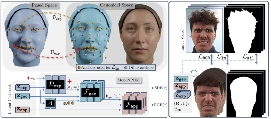
a) MonoNPHM

b) Tracking

Figure 2: Method overview: (a) Shows how MonoNPHM operates: First, points $x_{p}$ in posed-space are backward-warped through $\mathcal{F}_{\texttt{exp}}$ into canonical space (indicated by red star and arrow). Our canonical geometry and appearance fields are conditioned on facial anchors $\mathbf{a}_{c}$ (yellow and gray points in canonical space). Instead of conditioning $\mathcal{F}_{\texttt{app}}$ on canonical coordinates $(x_{c},\omega)$, we use hidden features $\mathbf{h}_{\texttt{geo}}$ extracted from the geometry network. (b) We approach tracking using SDF-based volumetric rendering [79] to build phomoetric and silhoutte terms. Additionally, we enforce a landmark loss by numerically inverting $\mathcal{F}_{\texttt{exp}}$ using iterative root finding (as indicated by the yellow arrow on the left).

2 Related Work

Mesh-based face models

Starting with the seminal work on 3DMMs [7], template-mesh-based PCA models [61, 46, 4, 87, 8] have been widely used for many application in computer graphics and vision. To relax the rigid linear assumption of PCA, subsequent efforts utilized variation auto-encoders(VAEs) [40], generative adversarial networks (GANs) [28], and diffusion models [30] to replace the PCA-basis underlying classical mesh-based 3DMMs [66, 27, 82, 78, 43, 23, 55].

3D face reconstruction from RGB

Reconstructing the 3D geometry of a head from RGB images or videos is a fundamental problem in computer vision. Standard approaches optimize the parameters of a 3DMM based on the 2D input [3, 25, 82, 76]. Optimizing the parameters from arbitrary poses, especially in the presence of occlusions and strong shadows, is a very challenging problem. Learning-based methods address this issue by training neural networks to predict the face representation from the input images [17, 70, 75, 48, 19]. In order to model details beyond the 3DMM template, such as wrinkles, several efforts utilize shape-from-shading [24, 33, 72] while others model facial details as displacements maps [14, 20, 44, 35]. Instead of relying on a fixed-topology template mesh, we approach 3D reconstruction from RGB inputs using neural-field-based parametric head models, allowing for the representation of complete human heads with varying topologies.

Neural field-based face models

Recent advances on neural fields [81], have shown impressive results on geometry reconstruction and generation [56, 51, 62, 83, 79], neural radiance fields (NeRFs) [52, 53, 15, 38], and dynamic scene reconstructions [57, 58, 42, 71, 2, 32]. Such techniques have been recently used in the context of 3D generative models [11, 12, 80, 5], and NeRF-based parametric models [77, 31, 94, 9, 10] to generate high-fidelity heads that can be rendered from different views. Others have focused on highly detailed geometry representation [85, 88, 26, 86, 89], design a diffusion prior for robust reconstruction from depth sensors [73], and facilitate few-shot 3D reconstruction from RGB images using a mixture of model-based fitting and test-time fine-tuning of model parameters [65, 47, 9]. Closer to our work, [47] is able to reconstruct an animatable head avatar from a single image in the wild. In this work, however, we focus on dynamic 3D reconstruction from monocular RGB videos by explicitly modeling the deformations, which allows us to obtain correspondences across the video.

Person-specific head avatars

To escape the limitation of generalizing parameter space, methods for person-specific avatars from monocular videos, have shown impressive results. These methods usually incorporate a 3DMM to introduce control in the neural implicit representation [22, 1, 96, 90, 93, 50, 63]. However, they lack generalization and as such, require to be trained per video, in contrast, to our method that generalizes across identities and expressions.

A different line of work focuses on the construction of photo-realistic avatars from abundant multi-view video recordings [50, 63, 41, 69].

3 MonoNPHM

Our work aims at dynamic 3D Face reconstruction in monocular RGB videos. We approach this heavily under-constrained task using model-based photometric tracking through inverse SDF-based rendering. In this section we describe the construction of our underlying, neural field-based model, MonoNPHM, illustrated in Fig. 2, along with its disentangled parametric spaces for shape (Sec. 3.1), appearance (Sec. 3.2) and expression information (Sec. 3.3). In Sec. 4 we propose a model-based dynamic 3D reconstruction algorithm, based on MonoNPHM.

3.1 Canonical Geometry Representation

We represent the head geometry in canonical facial expression, as described by latent code $\mathbf{z}_{\texttt{geo}}$, using a neural SDF

$$\mathcal{F}_{\texttt{geo}}:\mathbb{R}^{3+d_{\texttt{geo}}}\rightarrow\mathbb{R}^{1},x_{c}\mapsto\text{SDF}(x_{c}),$$ (1)

operating on points $x_{c}$ in canonical space. Such an implicit representation provides the necessary topological flexibility to describe complete heads, including hair.

We follow NPHM [26] and compose $\mathcal{F}_{\texttt{geo}}$ as an ensemble of local MLPs

$$\mathcal{F}_{\texttt{geo}}(x_{c},\mathbf{z}_{\texttt{geo}})\!=\!\sum_{k\in\mathcal{N}_{x_{c}}}w_{k}(x_{c},\mathbf{a}_{c}^{k})f_{\texttt{geo}}^{k}(x_{c}\!-\!\mathbf{a}^{k}_{c};\mathbf{z}_{\texttt{geo}}),$$ (2)

which are centered around facial anchor points $\mathbf{a}_{c}^{k}=\mathcal{A}(\mathbf{z}_{\texttt{geo}})\in\mathbb{R}^{65\times 3},$ that are predicted by a small MLP $\mathcal{A}$ based on the geometry code $\mathbf{z}_{\texttt{geo}}$. Therefore, the anchor positions constitute an integral part of the pipeline and provide an important discrete structure which we leverage as a landmark loss for monocular tracking in Sec. 4.4.

For this purpose we design an anchor layout consisting of $65$ points, s.t. the most important landmarks of common detectors coincide with anchor points, as shown in Fig. 2. To account for the increased number of anchors, we restrict the computation to the bipartite $k$NN-graph from $x_{c}$ to its $8$ nearest anchors $\mathcal{N}_{x_{c}}$, Compared to NPHM, which evaluates all local MLPs, in this case 65, this is more than an eight-fold reduction in memory. To account for the non-uniform spatial arrangement of anchors, we re-scale $w_{k}$ for each neighborhood separately. Details are provided in our supplementary material.

3.2 Canonical Appearance Representation

We model appearance changes between subjects using separate latent codes $\mathbf{z}_{\texttt{app}}$, that condition a texture field $\mathcal{F}_{\texttt{app}}$.

To emphasize the dependence of appearance on the geometry, we incorporate a strong connection between the two networks, similar to PhoMoH [86]. Our motivations come from the fact that an appearance space, which is completely independent of the geometry, could reconstruct the observed color images without providing meaningful gradients for the latest geometry codes.

To this end, we condition our texture field $\mathcal{F}_{\texttt{app}}$, on features $\mathbf{h}_{\texttt{geo}}(x_{c})\in\mathbb{R}^{16}$ which are extracted from the last layer of the geometry MLP $\mathcal{F}_{\texttt{geo}}$ using two narrow linear layers. As illustrated in Fig. 2, $\mathcal{F}_{\texttt{app}}$ follows the same local structure as our geometry network, i.e. local appearance MLPs

$$f_{\texttt{app}}^{k}(\mathbf{h}_{\texttt{geo}}^{k}(x_{c});\mathbf{z}_{\texttt{app}})\in[0,255]^{3}$$ (3)

are blended using the same weights as in Eq. 2. As we will show later in Sec. 5.4, removing the dependence of $\mathcal{F}_{\texttt{app}}$ on spatial coordinates $x_{c}$ and using features $\mathbf{h}_{\texttt{geo}}(x_{c})$ instead, is beneficial for RGB-based 3D reconstruction.

3.3 Representing Dynamics

While both previous components operate in canonical space, it is the task of our deformation network

$$D_{\texttt{exp}}:\mathbb{R}^{3+d_{\texttt{exp}}+d_{\texttt{geo}}}\rightarrow\mathbb{R}^{3},x_{p}\mapsto x_{c}$$ (4)

to backward-warp points $x_{p}$ in posed space into canonical coordinates $x_{c}$. Such a formulation implies that all changes in the geometry and appearance fields between two expressions can be explained through a deformation of space.

To relieve this strong assumption, we relax the formulation by adding hyper-dimensions, or ambient dimensions, [58] to the output of the deformation network, i.e. $D_{\texttt{exp}}(x_{p};\mathbf{z}_{\texttt{exp}},\mathbf{z}_{\texttt{geo}})=(x_{c},\omega)\in\mathbb{R}^{3+h}$, where $h$ is the number of hyper-dimensions (in practice we use $h=2$). Consequently, $\mathcal{F}_{\texttt{geo}}$ is provided with canonical coordinates and hyper-coordinates $\omega$, which increase the dynamic capacity of the overall network. Fig. 5 demonstrates the topological issues that arise without using hyper-dimensions.

Following previous work [54, 26], $\mathcal{F}_{\texttt{exp}}$ is conditioned on both $\mathbf{z}_{\texttt{exp}}$ and $\mathbf{z}_{\texttt{geo}}$ since the identity information is relevant to find correct correspondences between $x_{p}$ and $x_{c}$.

3.4 Training

We train all model components and latent codes end-to-end using an auto-decoder formulation [56]. Given a public dataset consisting of high-quality textured 3D scans [26], we sample points $x_{p}$ near the mesh surface and pre-compute $\text{SDF}(x_{p})$ and $\text{RGB}(x_{p})$ values for direct supervision of our geometry and color fields. Conceptually, we optimize for model parameters $\Theta$ and latent codes $\mathcal{Z}$

$$\underset{\mathcal{Z},\Theta}{\mathrm{argmin}}\! \sum\limits_{s\in S,e\in E_{s}}\lambda_{\text{SDF}}|\mathcal{F}_{\texttt{geo}}(\mathcal{F}_{\texttt{exp}}(x_{p}))-\text{SDF}(x_{p})|+$$ (5)

$$\lambda_{\text{RGB}}|\mathcal{F}_{\texttt{app}}(\mathbf{h}_{\texttt{geo}}(x_{c}))-\text{RGB}(x_{p})|+\lambda_{\text{reg}}\mathcal{L}_{\text{reg}},\quad$$

where $\mathcal{L}_{\textbf{reg}}$, among others, imposes regularization on all latent codes, supervises anchor predictions, and regularizes deformations and predicted hyper-dimensions to be small. We provide more details about the training and network architectures in our supplementary document.

4 3D Dynamic Face Reconstruction

Our main goal is tracking heads in the parametric space of MonoNPHM, in the case of a single, monocular RGB input video. In such a challenging scenario, it is essential that a strong, but expressive, model-prior can guide the optimization through the often under-constrained task. We conceptually visualize this task in Fig. 2. Given a video sequence of RGB frames $\{I_{1},\dots I_{T}\}_{t=1}^{T}$, associated silhouettes $\{S_{1},\dots S_{T}\}_{t=1}^{T}$ and 2D facial landmarks $\{L_{1},\dots,L_{T}\}_{t=1}^{T}$ we aim to reconstruct model parameters $\phi=\{\mathbf{z}_{\texttt{app}},\mathbf{z}_{\texttt{geo}}\}\cup\{\mathbf{z}_{\texttt{exp}}\}_{t=1}^{T}$, composed of time-invariant codes $\mathbf{z}_{\texttt{geo}}$ and $\mathbf{z}_{\texttt{app}}$, as well as, per frame expression codes $\mathbf{z}_{\texttt{exp}}^{t}$. We solve the tracking task by minimizing the energy

$$\underset{\phi,\zeta,\Pi}{\mathrm{argmin}}\sum_{t=1}^{T}\mathcal{L}_{\texttt{RGB}}^{t}+\lambda_{\texttt{sil}}\mathcal{L}_{\texttt{sil}}^{t}+\lambda_{\texttt{lm}}\mathcal{L}_{\texttt{lm}}^{t}+\lambda_{\texttt{reg}}\mathcal{L}_{\texttt{reg}}^{t}$$ (6)

with respect to latent codes $\phi$, head poses $\Pi=\{\mathbf{R}_{t},\mathbf{t}_{t}\}_{t=1}^{T}$, as well as, lighting parameters $\zeta\in\mathbb{R}^{9}$ of a 3-band spherical harmonics approximation [64].

The data term of our energy contains a pixel-level RGB loss $\mathcal{L}_{\texttt{RGB}}$ and silhouette loss $\mathcal{L}_{S}$, as explain in Secs. 4.1, 4.2 and 4.3, and a landmark loss $\mathcal{L}_{\texttt{lm}}$ for coarse guidance of the expression (see Sec. 4.4). We describe our regularization term and optimization strategy in Sec. 4.5 and Sec. 4.6, respectively.

4.1 Rendering Formulation

To relate the 3D neural field, parameterized by the latent codes, with the 2D observations, we perform volumetric rendering in posed space. Given intrinsic camera parameters $K$, we transfer the head pose into an extrinsics matrix $E_{t}=[\mathbf{R}_{t}|\mathbf{t}_{t}]$, and shoot a ray $r_{p}(\tau)=o+\tau\cdot d$ into the scene at time $t$. Samples along the ray are warped into canonical space

$$r_{c}(\tau)=D_{\texttt{exp}}(r_{p}(\tau);\mathbf{z}_{\texttt{exp}}^{t},\mathbf{z}_{\texttt{geo}}).$$ (7)

Consequently, we infer SDF values $\mathcal{F}_{\texttt{geo}}(r_{c}(\tau);\mathbf{z}_{\texttt{geo}})$ in caonical space. For volume rendering, we rely on the formulation of NeuS [79] to transfer SDF values along a ray into rendering densities $\sigma(r_{c}(\tau))$. In total, predicted RGB values $c(\tau)$ along a ray are aggregated into pixel colors

$$\hat{I}_{t}(r)\!=\!\int_{\tau_{n}}^{\tau_{f}}\!w(\tau)c(\tau)\!d\tau$$ (8)

using volume rendering [36, 52]. Here, rendering weights $w(\tau)$ and the accumulated transmittance $T(\tau)$ are defined as follows:

$$w(\tau)=T(\tau)\sigma(r_{c}(\tau)),~{}\text{and}~{}T(\tau)=e^{-\int_{\tau_{n}}^{\tau}\sigma(r_{c}(s))ds}.$$ (9)

4.2 Spherical Harmonics Shading

To bridge the domain gap between our albedo appearance space, and in-the-wild lighting effects, we include a 3-bands spherical harmonics as a simple approximation for the scene lighting [64]. Thus, we obtain shaded RGB predictions

$$c(\tau)=\text{SH}_{\zeta}(n(\tau))\mathcal{F}_{\texttt{app}}\!\left(\textbf{h}_{\texttt{geo}}(r_{c}(\tau));\mathbf{z}_{\texttt{app}}\right)$$ (10)

by multiplying predicted colors with the spherical harmonics term, parameterized by $\zeta\in\mathbb{R}^{9}$. For this, we use world space normals

$$n(\tau)=\mathbf{R}_{t}\nabla_{x_{p}}\mathcal{F}_{\texttt{geo}}(x_{c};\mathbf{z}_{\texttt{geo}}),$$ (11)

where the dependence on $x_{p}$ is included in the relation $x_{c}=\mathcal{F}_{\texttt{exp}}(x_{p};\mathbf{z}_{\texttt{exp}},\mathbf{z}_{\texttt{geo}})$. We show the importance of accounting for lighting effects in Sec. 5.4.

4.3 Rendering Losses

The most important term in our inverse rendering is the color loss $\mathcal{L}_{\texttt{RGB}}^{t}=\operatorname{MAE}(\hat{I}_{t},I_{t})$, which measures the average L1-loss over all pixels in the foreground region, between predicted image colors $\hat{I}_{t}$ and observed images $I_{t}$.

Additionally, we supervise the silhouette $S_{t}$ using an average binary cross-entropy loss $\mathcal{L}_{\texttt{sil}}^{t}=\operatorname{BCE}(\hat{S}_{t}(r),S_{t}(r))$ over all pixels, with predicted forground

$$\hat{S}_{t}=\int_{\tau_{n}}^{\tau_{f}}w(\tau)d\tau.$$ (12)

4.4 Landmark Loss

Next to the above-mentioned rendering losses we observe that the optimization can get stuck in local minima for extreme mouth movements. We address this issue by incorporating a landmark loss, a common practice in face tracking.

For this purpose, we exploit the structure of the underlying NPHM model that is offered through its anchor points $\mathcal{A}(\mathbf{z}_{\texttt{geo}})=\mathbf{a}_{c}$. We determine the anchor positions $\mathbf{a}_{p}^{t}$ in posed space that satisfy

$$0={\mathbf{a}_{c}^{t}}-\mathcal{D}_{\texttt{exp}}({\mathbf{a}_{p}^{t}};\mathbf{z}_{\texttt{exp}},\mathbf{z}_{\texttt{geo}})$$ (13)

using iterative root finding [16], i.e. the backward deformation field is inverted through a numerical procedure. To coarsely guide $\mathbf{z}_{\texttt{exp}}$ during tracking we enforce

$$\mathcal{L}_{\text{lm}}=\operatorname{MSE}(\pi_{K,E_{t}}({\mathbf{a}_{p}^{t}}),L_{t}),$$ (14)

which measures the screen-space distance between detected landmarks $L_{t}$ and projected posed anchors, where $\pi_{K,E_{t}}$ denotes a perspective projection using camera intrinsics $K$ and extrinsics $E_{t}$.

4.5 Regularization

We encourage the latent codes to stay within a well-behaved parameter range, which is also enforced during training:

$$\mathcal{L}_{\text{prior}}=\|\mathbf{z}_{\texttt{geo}}\|^{2}+\lambda_{\texttt{app}}\|\mathbf{z}_{\texttt{app}}\|^{2}+\frac{\lambda_{\texttt{exp}}}{T}\sum_{t}\|\mathbf{z}_{\texttt{exp}}\|^{2}.$$ (15)

Additionally, we use the symmetry loss from NPHM [26] on the local latent codes contained in $\mathbf{z}_{\texttt{geo}}$ and $\mathbf{z}_{\texttt{app}}$, and enforce temporal smoothness on time-dependent parameters

$$\mathcal{L}_{\text{smooth}}=\text{TV}(\mathbf{z}_{\texttt{exp}})+\lambda_{\text{rot}}\text{TV}(\mathbf{R}_{t})+\lambda_{\text{trans}}\text{TV}(\mathbf{t}_{t}).$$ (16)

4.6 Optimization Strategy

We optimize Eq. 6 using stochastic gradient descent (SGD) and the Adam optimizer [39]. We initialize all latent codes as zeros, $\zeta$ is initialized as uniform lighting from all directions, and head poses $\mathbf{R}_{t},\mathbf{t}_{t}$ are initialized from a tracked FLAME model.

We start our optimization by separately optimizing the first frame, and then optimize for the remaining frames sequentially in a frame-by-frame fashion, where $\mathbf{z}_{\texttt{geo}}$, $\mathbf{z}_{\texttt{app}}$, and $\zeta$ remain frozen. This strategy provides good estimates over all parameters and serves as initialization for our main stage, where we optimize over all parameters jointly. For each optimization step a random timestep $t$ and random rays for the rendering losses are sampled. Our smoothness loss is computed between the neighboring frames $t-1$ and $t+1$.

5 Results

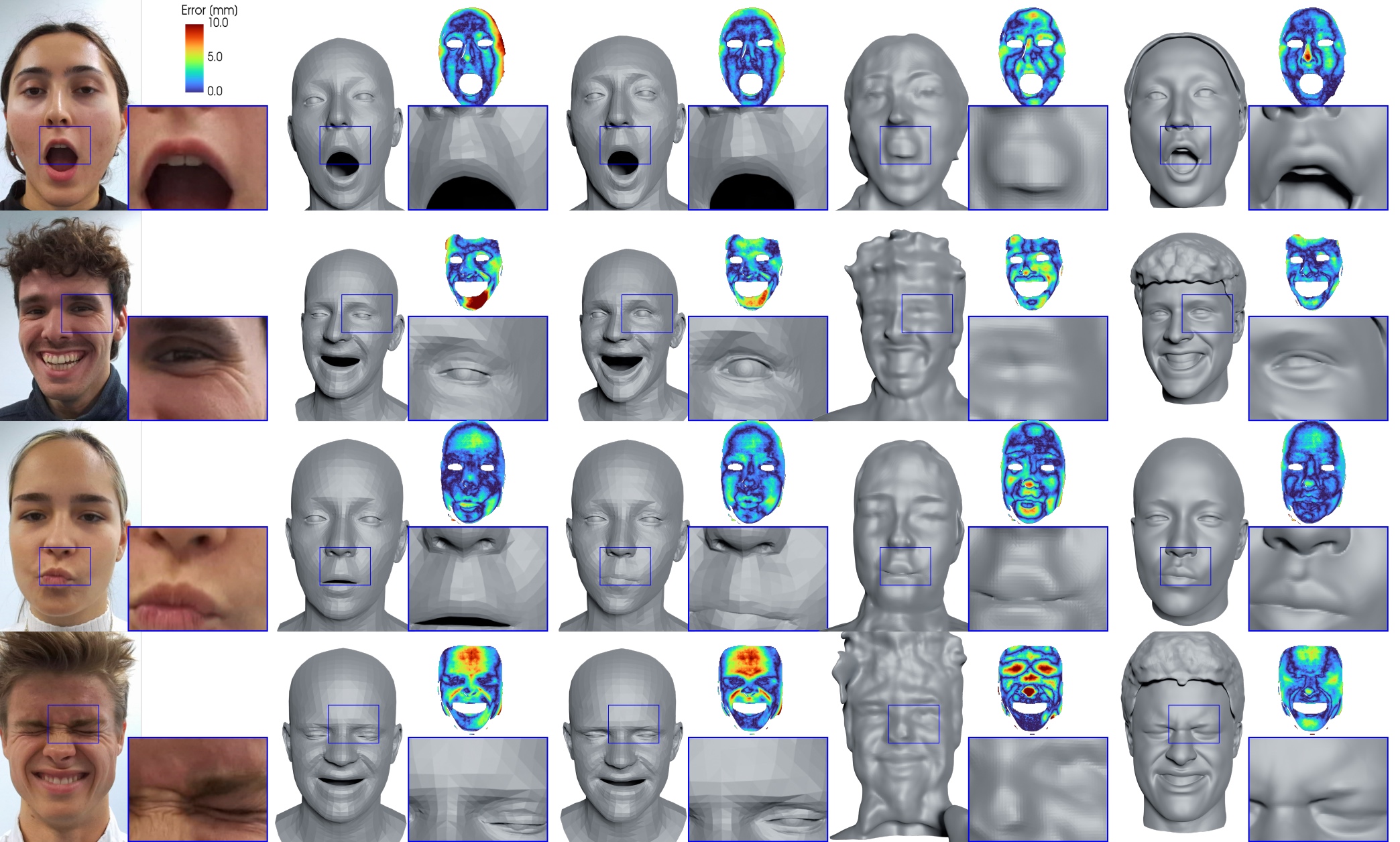
Input RGB Frame

DECA [19]

MICA Tracker [95]

IMavatar [90]

Ours

Figure 3: Comparison of the 3D reconstruction quality from monocular RGB videos against our baseline. We show error maps with color-coded point-to-mesh distance from ground truth Kinect depth to the reconstructed meshes.

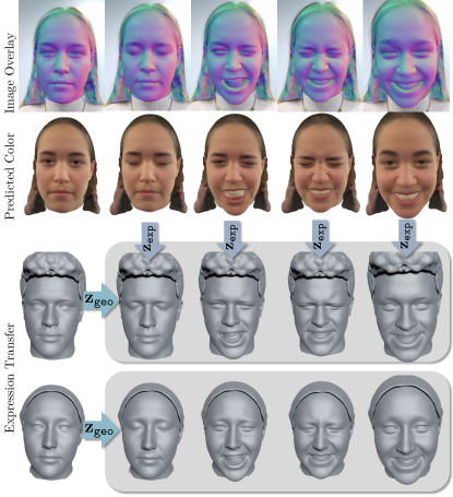
Figure 4: Temporal Reconstructions: We show five reconstructions from same sequence (top two rows). A 50-50 overlay (top row) between reconstructed normals and the input images demonstrates accurate alignment in the image space. The bottom two rows show cross-reenactment by transferring the reconstructed expression codes to two previously reconstructed subjects.

To evaluate our goal of dynamic face reconstruction, we record 20 Kinect sequences in a casual setting, for a lack of publicly available alternatives. The RGB sensor serves as input, while the depth sensor allows for a geometric evaluation. We record 5 participants (3 female, 2 male) under a wide range of facial expressions, emotions and include one talking sequence. All participants signed agreements compliant with GDPR requirements. We record each sequence for 12 seconds at 15 frames per second, resulting in 180 frames per sequence.

5.1 Metrics

We report unidirectional $L_{1}$-Chamfer distance in meters from the back-projected depth map to the reconstructions, which cover the complete head. Similarly, we report the unidirectional cosine-similarity of normals. Additionally, we measure the recall [74], i.e. the percentage of ground truth points that are covered by at least one point on the reconstruction w.r.t. to a given threshold distance.

Evaluation Protocol   To eliminate any remaining depth ambiguity, we optimize for a similarity transform from reconstructed mesh to ground truth point cloud using ICP [6]. To exclude the sensor noise of the regions inside the mouth and eyes and to account for differences between the compared methods, we remove these regions, as well as the hair and neck region, using facial segmentation [92]. We visualize the resulting ground truth point clouds in Fig. 3, which are color-coded according to the Chamfer distance.

5.2 Baselines

MICA tracker [95] Using a 3DMM as a model prior is the most prominent approach to 3D face tracking. We use the state-of-the-art facer tracker from MICA [95], which is based on FLAME [46], as a representative of PCA-based tracking approaches.

DECA [19] DECA is a feed-forward CNN that predicts FLAME parameters and offsets, and is trained in a self-supervised fashion on in-the-wild images, thereby obtaining robustness to real-world lighting conditions.

IMavatar [90] IMavatar is representative of the per-scene avatar reconstruction methods. Similar to our method, IMavatar uses neural fields to explain details beyond the capabilities of the underlying FLAME model. It merely uses a tracked FLAME model as guidance during optimization.

5.2.1 Implementation Details

Training MonoNPHM We implement our model in Pytorch [59] and utilize PytorchGeometric [21] to restrict computations in canonical space to the $k$ nearest anchors. We follow NPHM [26] and use 64 dimensions for the global latent codes involved in $\mathbf{z}_{\texttt{app}}$ and $\mathbf{z}_{\texttt{exp}}$. For the local codes we use 32 dimensions. For the expression codes $\mathbf{z}_{\texttt{exp}}$ we use 100 dimensions. We train our model for 2500 epochs, use a batch size of 64, and a learning rate of $5e^{-4}$ for the networks and $2e^{-3}$ for the latent codes. We train on the NPHM dataset  [26] using 4 NVIDIA RTX2080 GPUs with 12GB of VRAM taking roughly 52 hours until convergence. More details are provided in our supplementary.

Data Pre-Processing We perform several common pre-processing steps to remove parts of the observed images that are not included in our learned prior and detect landmarks. Namely, we rely on face detection [18], facial landmark detection [34], semantic segmentation to remove the torso [92], as well as, video matting [37] to remove the background. For all baselines, we follow their proposed pre-processing pipeline.

Tracking For each step of SGD we randomly sample 500 rays. During volume rendering, we randomly sample 32 coarse samples, and additional 32 samples using importance sampling. We start with a large variance for the NeuS [79] rendering, which is decayed over time to concentrate tightly around the surface. We perform 250 optimization steps for the first frame, and 60 steps per frame otherwise. To build forward correspondences for our landmark loss, we use 5 random initializations for iterative root finding. More details are provided in the supplementary.

Our optimization operates at roughly 1.2 frames per minute. As a comparison, the MICA tracker can track 2 frames per minute using the default settings, and IMavatar operates at roughly 0.4 frames per minute.

Method	$L_{1}$-Chamfer $\downarrow$	N. C. $\uparrow$	Recall@2.5mm $\uparrow$
DECA [19]	$0.0034$	$0.917$	$0.644$
MICATracker [95]	$0.0030$	$0.932$	$0.654$
IMavatar [90]	$0.0054$	$0.888$	$0.625$
Ours	0.0024	$\mathbf{0.940}$	$\mathbf{0.785}$

Table 1: Comparison of 3D face reconstruction from monocular RGB videos. The chamfer distance is reported in meters.

5.3 Tracking Results

We compare MonoNPHMto our baselines by fitting each model to all the 20 monocular RGB sequences individually. We report quantitative and qualitative results in Tab. 1 and Fig. 3, respectively. For results on the complete sequences, we kindly refer to our supplementary video. Fig. 3 shows that MonoNPHM reconstructs important details about the face shape and expressions, that significantly help to recognize the identity and interpret the reconstructed emotion correctly. Compared to the 3DMM-based approaches, DECA and the MICA tracker, MonoNPHM is capable of reconstructing complete heads, including the mouth inside and hair. IMavatar, on the other hand, suffers from its increased representational capacity compared to FLAME, due to the difficulty of task. The quantitative evaluation reported in Tab. 1 confirms these findings.

Additionally, we show qualitative results for five frames of the same sequence in Fig. 4, to demonstrate temporal consistency and the alignment of our reconstructed geometry against the input sequence in screen space. Alongside, we show the predicted color images $\hat{I}$ of MonoNPHM, to give further insights into our rendering loss $\mathcal{L}_{\texttt{RGB}}$, which mainly drives our optimization. Finally, we perform cross-reenactment by transferring the reconstructed latent codes $\mathbf{z}_{\texttt{exp}}$ to the identity codes $\mathbf{z}_{\texttt{geo}}$ and $\mathbf{z}_{\texttt{app}}$ from another participant. Visually, the resulting reenactments capture the contents of the original expression to a high degree.

5.4 Ablations

Method	$L_{1}$-Chamfer $\downarrow$	N. C. $\uparrow$	Recall@2.5mm $\uparrow$
w/ sphere tracing	$0.0033$	$0.905$	$0.674$
w/o spher. harm.	$0.0028$	$0.923$	$0.718$
w/o $\mathcal{L}_{\texttt{lm}}$	$0.0027$	$0.939$	$0.745$
w/o color comm.	$0.0028$	$0.933$	$0.735$
w/ global MLP	$0.0026$	$\mathbf{0.940}$	$0.768$
Ours	0.0024	$\mathbf{0.940}$	$\mathbf{0.785}$

Table 2: Ablation experiments isolating single components of our tracking approach (first 3 rows), and of our architecture (second section). See Sec. 5.4 for details on the individual experiments.

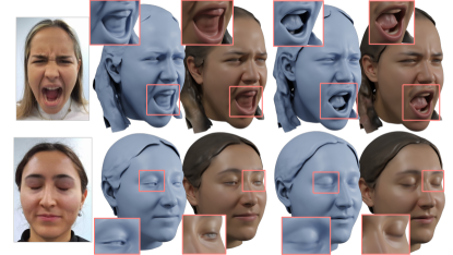
RGB

wo/ hyper-dims.

w/ hyper-dims.

Figure 5: Effect of Hyper-Dimensions: Without the addition of hyper-dimensions, the backward deformation model cannot accurately reconstruct geometry and color for topologically challenging expressions, e.g. opening of mouth and closing of eyes.

We support several of our claims by ablating individual components on the same 20 Kinect sequences. We report quantitative results in Tab. 2 and refer to our supplementary for a qualitative comparison.

Tracking Algorithm   Firstly, we show that NeuS-style volume rendering [79], instead of the sphere-tracing-based rendering of implicit surfaces [83], is essential for the success of our tracking approach. Second, the use of spherical harmonics is crucial to account for lighting conditions that vastly differ from our training data. Otherwise, the RGB loss is dominated by lighting effects that our model cannot explain. Lastly, we note that without using the landmark loss $\mathcal{L}_{\texttt{lm}}$ our optimization often performs similarly well, but tends to get stuck in local minima, if large and fast mouth movements, e.g. during shouting, are encountered.

The effect of $\mathbf{h}_{\texttt{geo}}$   Furthermore, we show the significance of removing the communication channel between geometry and color networks. To this end, we train a model that uses canonical coordinates $x_{c}$ instead of $\mathbf{h}_{\texttt{geo}}(x_{c})$ as input to the local color MLPs defined in Eq. 3. We hypothesize that for such a model, gradients through our most important loss $\mathcal{L}_{\texttt{RGB}}$ are less informative for $\mathbf{z}_{\texttt{geo}}$ and $\mathbf{z}_{\texttt{exp}}$.

Local vs Global MLPs   Additionally, we ablate the effect of using the local MLP ensemble from NPHM [26] against a simpler architecture, that represents $\mathcal{F}_{\texttt{geo}}$ and $\mathcal{F}_{\texttt{app}}$ using a global MLP. To account for good tracking of extreme expressions, we find that the landmark loss is equally important for this global architecture. To this end, we include the anchor prediction MLP $\mathcal{A}$ into this ablation experiment, such that the usage of $\mathcal{L}_{\texttt{lm}}$ becomes viable. Doing so, we are able to associate $\mathbf{a}_{c}$ with $\mathbf{z}_{\texttt{geo}}$, and achieve good tracking performance, with slightly fewer geometric details, as reflected in the metrics.

Effect of Hyper-Dimensions.   Finally, in Fig. 5 we highlight the importance of using hyper-dimensions for correctly representing topologically challenging expressions, such as the closing of the eyes and opening of the mouth.

6 Limitations

In our experiments, we show that MonoNPHM can reconstruct high-quality human heads from monocular videos; however, at the same time, we believe that there are still several limitations and opportunities for future work. For instance, while spherical harmonics can be used to account for simple lighting conditions without increasing the model complexity, we believe that reconstructions could be improved by addressing lighting and shadows more thoroughly. Possible options are the inclusion of a more advanced shading model during volume rendering  [67], image-space delighting [84], as well as, CNN-based image encoders [19, 13]. Another limitation is our tracking speed. While this is partially explained by our unoptimized implementation that runs a full optimization for each frame, we believe that several advances can be made, e.g. using CNN-based initialization [60], coarse-to-fine optimization, faster neural-field backbones [53, 15] and second-order optimization for tracking [76].

7 Conclusion

In this work we have introduced MonoNPHM, a neural-field-based parametric face model, that represents faces using an SDF and texture field in canonical space, and represents movements using backward deformations, augmented with hyper-dimensions. We enforce a tight communication between appearance and geometry to facilitate efficient inverse rendering. By including explicit control points in our implicit geometry representation, we have developed a highly accurate 3D face tracking algorithm based on volumetric rendering for implicit surfaces. MonoNPHM achieves significantly more accurate 3D reconstruction on challenging monocular RGB videos, compared to all our baselines. We believe that our work makes the use of neural parametric head models much more accessible for many downstream tasks. We hope that our work inspires more research to explore the use of neural-field-based parametric models and develop the necessary toolsets that are already available for classical 3DMMs.

Acknowledgements

This work was funded by Synthesia and supported by the ERC Starting Grant Scan2CAD (804724), the German Research Foundation (DFG) Research Unit “Learning and Simulation in Visual Computing”. We would like to thank our research assistants Mohak Mansharamani and Kevin Qu, and Angela Dai for the video voice-over.

Appendix

Appendix A Overview

This supplementary document provides additional implementation details on our network architecture (Secs. B.1 and B.2), training (Sec. B.3) and tracking strategy (Sec. B.4).

Additionally, we present more qualitative results (Appendix C) and discuss our ablation experiments (Sec. C.2).

We kindly suggest the reviewers watch our supplementary video, for a temporally complete visualization of the tracked sequences.

Appendix B Implementation Details

In Sec. B.1 we provide details about the individual network components of MonoNPHM. Sec. B.2 describes how we implement a memory efficient variant of the MLP ensemble proposed in [26].

B.1 Network Architectures

Some of mentioned details in this subsection require detailed knowledge about NPHM [26].

Expression Network

To represent our backward deformation field $\mathcal{F}_{\texttt{exp}}$ we use a 6-layer MLP with a width of 400. The expression codes $\mathbf{z}_{\texttt{exp}}$ are 100 dimensional. The dependence on $\mathbf{z}_{\texttt{geo}}$ is bottlenecked by a linear projection to 16 dimensions, as proposed in [26].

Geometry Network

Our local geometry MLPs $f_{\texttt{geo}}^{k}$ have 4 layers and a width of 200. Out of the 65 anchors, 30 are symmetric, meaning that the ensemble consists of $64-30=34$ MLPs. Note, however, that the spatial input of $f_{\texttt{geo}}^{k}$ is augmented with the predicted hyper-dimensions.

Appearance Network

Our appearance MLPs $f_{\texttt{app}}^{k}$ follow the same structure as $f_{\texttt{geo}}^{k}$, but receive extracted geometry features $\mathbf{h}_{\texttt{geo}}(x_{c})$ as input. $\mathbf{h}_{\texttt{geo}}$ is a two-layer MLP (widths 100 and 16), that maps the hidden features of the last layers of $f_{\texttt{geo}}^{k}$ to 16 dimensions.

Anchor Prediction

Compared to the anchor layout used in NPHM [26], we increase the number of anchors from 39 to 65, and rearrange them, such that the anchors coincide with the most important facial landmarks for tracking. Fig. 6 shows our anchor layout. The anchor prediction MLP $\mathcal{A}$ consists of 3 linear layers and has a hidden dimension of 64.

B.2 Efficient Implementation

To account for the computational burden of the increased number of anchors and added appearance MLPs, we prune the computations of the local MLP ensemble.

$k$NN Pruning

NPHM executes every MLP $f_{\texttt{geo}}^{k}$ for each query point $x_{c}$. Instead, we use Pytorch3D [68] to compute the 8 nearest neighbors $\mathcal{N}_{x_{c}}$ for each query. Then, we conceptualize the execution of local MLPs as a graph convolution, implemented using PytorchGeometric [21]. The graph convolution is restricted to $\mathcal{N}_{x_{c}}$ (see Eq. 2). In practice, this decreases the number of MLP executions for each query from 65 to 8 (the number of nearest neighbors). Hence, GPU memory demand is roughly reduced 8-fold

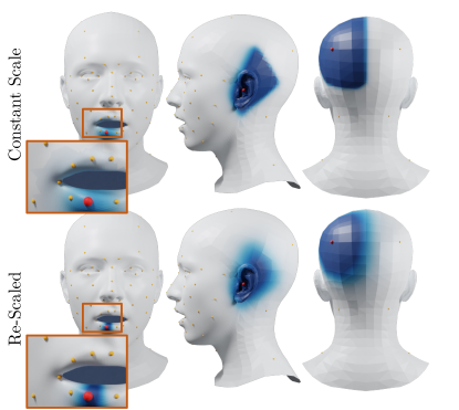
Figure 6: Re-Scaling $w_{k}$: We show weights $w_{k}$ for three different anchors (red) among all the 65 anchors (orange). The mesh surface is colored according to $w_{k}$ where white corresponds to a low value and blue to a large value. The bottom row shows our re-scaled weights compared to a constant scale (top row). Note the discontinuities on the top left, and the sharp decay on the top right.

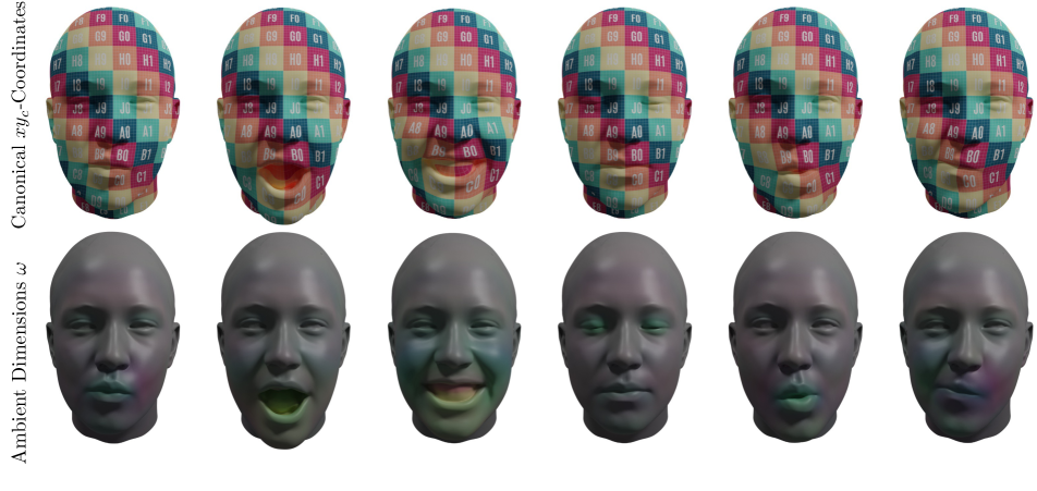
Figure 7: Deformation Consistency: We illustrate the behavior of our deformation network $\mathcal{F}_{\texttt{exp}}$, by visualizing the predicted canonical coordinates $x_{c}$ (top row) and hyper dimensions $\omega$ (bottom row) for 6 diverse frames of one tracked sequence. We use the $x$ and $y$ components of $x_{c}$ to index a checkerboard image, demonstrating that the semantics of the face’s surface are consistently deformed. To visualize $\omega\in\mathbb{R}^{2}$ we map it to the red and green channels, where $0$ corresponds to gray.

Re-Scaling $w_{k}$

For a given query point $x_{c}$ and local MLP associated to the anchor point $\mathbf{a}_{k}$, NPHM uses weights

$$w_{k}^{*}(x_{c},\mathbf{a}_{k})=\text{exp}\left(\frac{-\|x_{c}-\mathbf{a}_{k}\|_{2}}{2\sigma}\right),$$ (17)

and normalizes them to $w_{k}$ in order to blend the predictions of the individual MLPs. However, when restricting the computations to the set of nearest neighbors, such a constant-scale Gaussian weighting results in discontinuous for points on the boundary of Voronoi cells, i.e. when the set of nearest neighbors changes.

As demonstrated in the top left of Fig. 6, the influence of the highlighted anchor point exhibits a sharp boundary. This effect can be mitigated by reducing $\sigma$ to be significantly smaller than the size of the Voronoi cells. However, due to the non-uniform spatial arrangement of anchors, finding a single $\sigma$ that ensures smooth boundaries for all anchors is impossible.

Consequently, we vary

$$\sigma(x_{c})=\frac{1}{4}\underset{x\in\mathcal{N}_{x_{c}}}{\mathrm{max}}\|x_{c}-x\|_{2}$$ (18)

according to the set of nearest neighbors of $\mathcal{N}_{x_{c}}$. Doing so ensures that $w_{k}^{*}(x_{c},\mathbf{a}_{k})$ decays quickly enough to zero when approaching the boundaries of its Voronoi cell.

B.3 Training Details

B.3.1 Data Preparation

We use the 3D textured scans of the NPHM dataset [26] for training. To this and we sample points on the surface $\mathcal{S}_{\text{surf}}$ and near the surface $\mathcal{S}_{\text{near}}$, and define $\mathcal{S}_{\text{all}}=\mathcal{S}_{\text{surf}}\cup\mathcal{S}_{\text{near}}$. For $x_{p}\in\mathcal{S}_{\text{all}}$ we precompute its normal $n(x_{p})$ and color $\text{RGB}(x_{p})$. Additionally, we precompute samples $(x_{p},x_{c})\in\mathcal{S}_{\text{corr}}$ of corresponding points in posed and canonical space following [54] and using the provided registered meshes in the NPHM dataset.

B.3.2 Loss Functions

We train MonoNPHM in an end-to-end fashion, similar to ImFace [88] which jointly trains geometry and expression networks.

Geometry Supervision

The employed losses are similar to [29], however, adopted to dynamic objects similarly to [88]. Hence, the main losses for the geometry and expression supervision put constraints on the zero-level set through

$$\mathcal{L}_{\text{level-set}}=\sum_{x_{p}\in\mathcal{S}_{\text{surf}}}\|\mathcal{F}_{\texttt{geo}}(\mathcal{F}_{\texttt{exp}}(x_{p}))\|_{1}$$ (19)

and on the surface normals through

$$\mathcal{L}_{\text{n}}=\sum_{x_{p}\in\mathcal{S}_{\text{surf}}}\|\nabla_{x_{p}}\mathcal{F}_{\texttt{geo}}(\mathcal{F}_{\texttt{exp}}(x_{p}))-n(x_{p})\|_{2},$$ (20)

where we omit the dependence on latent codes for brevity. Additionally, we enforce the eikonal constraint

$$\mathcal{L}_{\text{eik}}=\sum_{x_{p}\in\mathcal{S}_{\text{all}}}\|\nabla_{x_{p}}\mathcal{F}_{\texttt{geo}}(\mathcal{F}_{\texttt{exp}}(x_{p}))-1\|_{2}.$$ (21)

To guide $\mathcal{F}_{\texttt{exp}}$ during the first half of training we include a correspondence loss

$$\mathcal{L}_{\text{corr}}=\sum_{(x_{p},x_{c})\in\mathcal{S}_{\text{corr}}}\|\mathcal{F}_{\texttt{exp}}(x_{p})-x_{c}\|_{1}.$$ (22)

On one side this provides direct expression supervision. On the other side $\mathcal{L}_{\text{corr}}$ also enforces the first 3 dimensions of the canonical space to behave as Euclidean as possible. This is not only desirable but also extremely important for the landmark loss $\mathcal{L}_{\texttt{lm}}$ to work. For the same reason, we regularize predicted hyper-dimensions $\omega=[{\mathcal{F}_{\texttt{exp}}}(x_{p})]_{\omega}$ to be small using

$$\mathcal{L}_{\text{hyper}}=\sum_{x_{p}\in\mathcal{S}_{\text{all}}}\|~{}[{\mathcal{F}_{\texttt{exp}}}_{\omega}(x_{p})]_{\omega}~{}\|_{2}.$$ (23)

In a similar fashion, we regularize predicted deformations to be small

$$\mathcal{L}_{\text{def}}=\sum_{x_{p}\in\mathcal{S}_{\text{surf}}}\|\mathcal{F}_{\texttt{exp}}(x_{p})-x_{p}\|_{2}.$$ (24)

Finally, we include the same regularization terms as [26], i.e. we constrain the norm of $\mathbf{z}_{\texttt{geo}}$ and $\mathbf{z}_{\texttt{exp}}$ and apply a symmetry loss on the symmetric parts of $\mathbf{z}_{\texttt{geo}}$.

Anchor Supervision

Anchor positions are directly supervised using

$$\mathcal{L}_{\mathcal{A}}=\|\mathbf{a}_{\text{gt}}-\mathcal{A}(\mathbf{z}_{\texttt{geo}})\|_{F}$$ (25)

where the ground truth anchor positions $\mathbf{a}_{\text{gt}}$ are extracted from the registered meshes in FLAME [46] topology, as provided by the NPHM dataset. Therefore, the anchors are supervised to follow the Euclidean coordinate system of the FLAME model. While this seems obvious, we note that without the necessary precautions imposed by $\mathcal{L}_{\text{corr}}$, $\mathcal{L}_{\text{def}}$, and $\mathcal{L}_{\text{hyper}}$, our canonical space becomes non-euclidean, similarly to [49, 45, 93].

Appearance Supervision

The appearance codes $\mathbf{z}_{\texttt{app}}$ and network $\mathcal{F}_{\texttt{app}}$ are jointly optimized alongside the geometry, by including

$$\mathcal{L}_{\text{app}}=\sum_{x_{p}\in\mathcal{S}_{\text{all}}}\|\mathcal{F}_{\texttt{app}}(\mathbf{h}_{\texttt{geo}}(\mathcal{F}_{\texttt{exp}}(x_{p}))-\text{RGB}(x_{p})\|_{1}$$ (26)

into our training. Similarly as before, we also regularize the norm of $\mathbf{z}_{\texttt{app}}$. We do not include a perceptual loss during training, as done in [86, 47], since we are focused on geometry reconstruction via inverse rendering, instead of photorealistic appearance.

B.3.3 Training Strategy

Using the above-mentioned losses, we train all networks and latent codes jointly in an auto-decoder fashion [56]. We use the Adam optimizer [39], and periodically divide the learning rates by half every 500 epochs, for a total of 2500 epochs and use a batch size of 64. We start with $lr_{\text{networks}}=0.0005$, $lr_{\text{lat-can}}=0.002$ and $lr_{\text{lat-exp}}=0.01$, for the network parameters, latent codes for canonical space and latent expression codes, respectively.

B.4 Tracking Details

We perform iterative root finding using 5 random samples normally distributed around the canonical anchor $\mathbf{a}_{k}$ of interest, as we experience similar convergence issues to [16] that are dependent on the initial position.

Since the inside of the mouth is subject to extreme shadows, far beyond what our simple lighting assumptions can explain, we use the predicted facial segmentation masks [91] to down-weigh the color loss $\mathcal{L}_{\texttt{RGB}}$ by a factor of 25 for that region.

Furthermore, we employ several mechanisms to encourage a coarse-to-fine optimization. First, we decay all learning rates of the employed Adam optimizer periodically throughout the optimization. The learning rate for the head pose and spherical harmonics parameters $\zeta$ start larger and decay faster compared to the learning rate of the latent codes. Second, we increase the inverse standard deviation from the NeuS [79] volume rendering formulation from $0.3$ to $0.8$. Therefore, the rendering densities are initially distributed widely around the surface, allowing for a large volume that receives gradients in the coarser stages of optimization. Third, the influence of the landmark loss $\mathcal{L}_{\texttt{lm}}$ is strongly decayed throughout the optimization progress. Initial epochs strongly rely on landmark guidance, while later ones are barely affected by it anymore. Additionally, we weigh the landmarks of the eyes, mouth and chin $100$ more then the remaining ones.

Appendix C Additional Qualitative Results

C.1 Additional Comparisons

Next to the results in the main paper and our supplementary video, we show additional qualitative comparisons against our baselines in Fig. 8. Note that each row shows a frame from a different sequence, which are reconstructed separately.

C.2 Ablations

While our main document only reported quantitative results of our ablation experiments, due to space reasons, Fig. 9 and our supplementary video show qualitative results. In the following we highlight some key insights from our ablation experiments:

Effect of $\mathcal{L}_{\texttt{lm}}$

Generally, our tracking performs well even when the landmark loss is disabled. However, some extreme expressions are completely missed without it, see the second column in Fig. 9.
Additionally, utilizing a landmark detector trained on large image collections of in-the-wild images provides some robustness against lighting and shadow effects.

Volume Rendering vs. Sphere Tracing

Utilizing sphere tracing [83], instead of a volumetric formulation [79], for differentiable SDF-based rendering results in reconstructions that are perceptively dissimilar to the subject. Additionally, we note that the sphere tracing sometimes gets stuck in local minima, where it is not able to remove hair geometry in front of the forehead, see columns four and five.

Spherical Harmonics

Since our model is trained on 3D scans, with albedo-like texture, accounting for lighting effects is important. Removing the spherical harmonics term, makes the task slightly ill-posed and generally results in worse reconstruction quality.

Color Communication

Conditioning the color MLP $\mathcal{F}_{\texttt{app}}$ directly on canonical spatial coordinates $x_{c}$ instead of geometry features $\mathbf{h}_{\texttt{geo}}(x_{c})$, gives the model extra freedom since both outputs are less correlated. For example in column 3 this results in a failure to separate the hair and cheek. Additionally, such a communication bottleneck was found to be beneficial for disentangling the geometry and appearance latent spaces [86].

Local vs. Global MLPs

Our MLPs modeling the SDF and texture field follow the local structure proposed in [26], i.e. we use an ensemble of local MLPs, each centered around its specific facial anchor points. Additionally, symmetric face regions are represented using the same MLP, but with mirrored coordinates. Our main motivation for choosing such an architecture are the facial anchors, which we exploit to formulate our landmark loss. We realized that it is also possible to use the same landmark loss while using global MLPs for both SDF and texture field. To this end, it is necessary to add the anchor prediction network $\mathcal{A}$ to the architecture, although the predicted anchors are not used anywhere else in that architecture. We find that training such a model is still capable of successfully associating the geometry code $\mathbf{z}_{\texttt{geo}}$ with plausible facial anchors. Nevertheless, the local MLP ensemble still learns a more detailed latent representation, which, for example, shows in the slightly blurry eye reconstructions in columns three and five.

Figure 8: Tracking Comparison: We show additional qualitative results of the monocular 3D reconstruction task. The error maps show the color-coded point-to-mesh distance from the back-projected Kinect depth to the reconstruction.

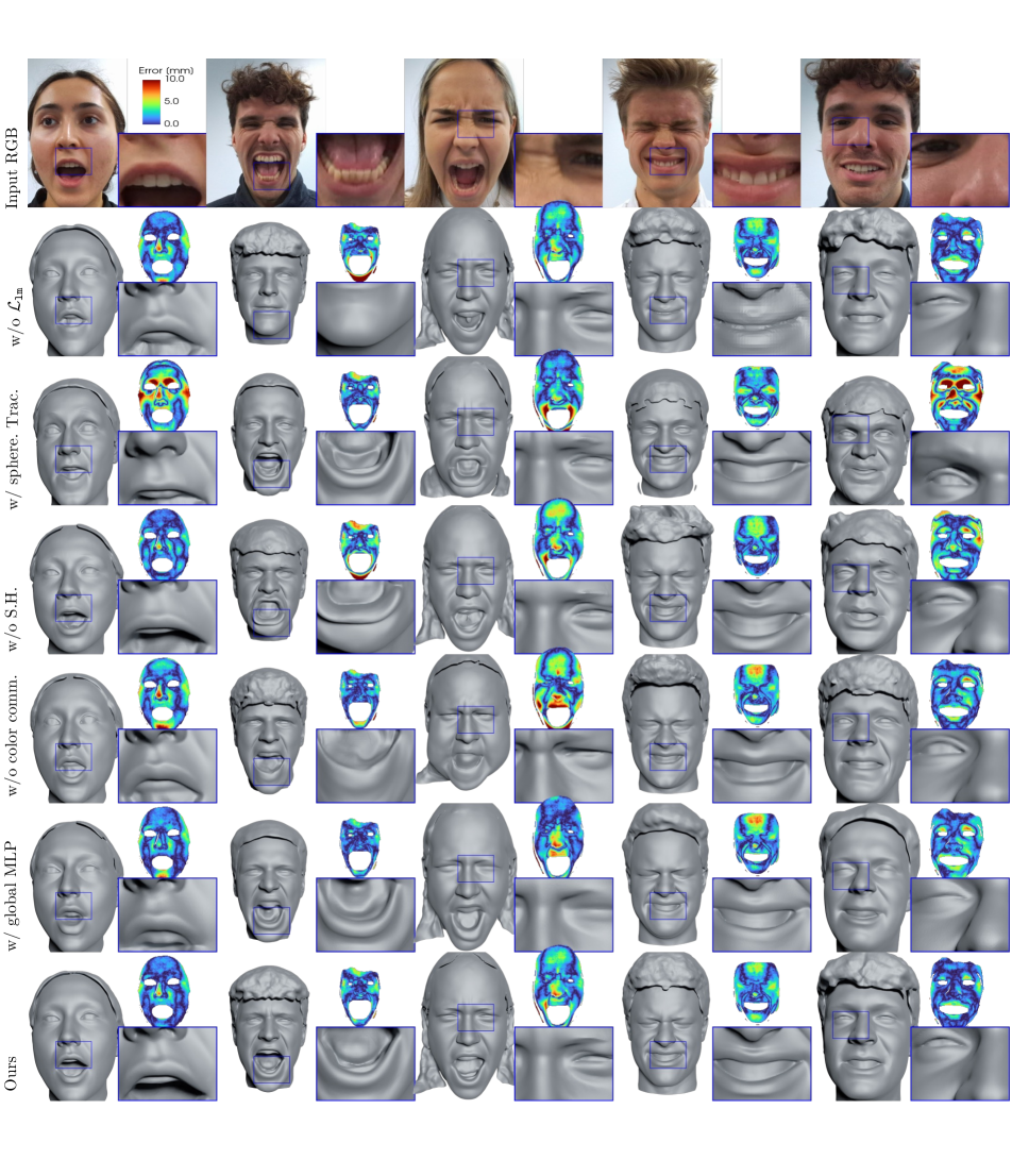
Figure 9: Ablation Results: Qualitative comparison of our ablation experiments, as quantitatively reported in 2. Rows and columns are transposed compared to our other result figures. The error maps show the color-coded point-to-mesh distance from the back-projected Kinect depth to the reconstruction. See Sec. C.2 for a description of our findings.

References

- Athar et al. [2022] ShahRukh Athar, Zexiang Xu, Kalyan Sunkavalli, Eli Shechtman, and Zhixin Shu. Rignerf: Fully controllable neural 3d portraits. In Proceedings of the IEEE/CVF Conference on Computer Vision and Pattern Recognition (CVPR), pages 20364–20373, 2022.
- Attal et al. [2023] Benjamin Attal, Jia-Bin Huang, Christian Richardt, Michael Zollhoefer, Johannes Kopf, Matthew O’Toole, and Changil Kim. HyperReel: High-fidelity 6-DoF video with ray-conditioned sampling. In Conference on Computer Vision and Pattern Recognition (CVPR), 2023.
- Bai et al. [2023] Haoran Bai, Di Kang, Haoxian Zhang, Jinshan Pan, and Linchao Bao. Ffhq-uv: Normalized facial uv-texture dataset for 3d face reconstruction. In Proceedings of the IEEE/CVF Conference on Computer Vision and Pattern Recognition, pages 362–371, 2023.
- Bao et al. [2021] Linchao Bao, Xiangkai Lin, Yajing Chen, Haoxian Zhang, Sheng Wang, Xuefei Zhe, Di Kang, Haozhi Huang, Xinwei Jiang, Jue Wang, Dong Yu, and Zhengyou Zhang. High-fidelity 3d digital human head creation from rgb-d selfies. ACM Transactions on Graphics, 2021.
- Bergman et al. [2022] Alexander W. Bergman, Petr Kellnhofer, Wang Yifan, Eric R. Chan, David B. Lindell, and Gordon Wetzstein. Generative neural articulated radiance fields. In NeurIPS, 2022.
- Besl and McKay [1992] P.J. Besl and Neil D. McKay. A method for registration of 3-d shapes. IEEE Transactions on Pattern Analysis and Machine Intelligence, 14(2):239–256, 1992.
- Blanz and Vetter [1999] Volker Blanz and Thomas Vetter. A morphable model for the synthesis of 3d faces. In Proceedings of the 26th annual conference on Computer graphics and interactive techniques, pages 187–194, 1999.
- Booth et al. [2018] James Booth, Anastasios Roussos, Allan Ponniah, David Dunaway, and Stefanos Zafeiriou. Large scale 3d morphable models. International Journal of Computer Vision, 126(2):233–254, 2018.
- Bühler et al. [2023] Marcel C. Bühler, Kripasindhu Sarkar, Tanmay Shah, Gengyan Li, Daoye Wang, Leonhard Helminger, Sergio Orts-Escolano, Dmitry Lagun, Otmar Hilliges, Thabo Beeler, and Abhimitra Meka. Preface: A data-driven volumetric prior for few-shot ultra high-resolution face synthesis. In Proceedings of the IEEE/CVF International Conference on Computer Vision (ICCV), pages 3402–3413, 2023.
- Cao et al. [2022] Chen Cao, Tomas Simon, Jin Kyu Kim, Gabe Schwartz, Michael Zollhoefer, Shun-Suke Saito, Stephen Lombardi, Shih-En Wei, Danielle Belko, Shoou-I Yu, Yaser Sheikh, and Jason Saragih. Authentic volumetric avatars from a phone scan. ACM Trans. Graph., 41(4), 2022.
- Chan et al. [2020] Eric Chan, Marco Monteiro, Petr Kellnhofer, Jiajun Wu, and Gordon Wetzstein. pi-gan: Periodic implicit generative adversarial networks for 3d-aware image synthesis. In arXiv, 2020.
- Chan et al. [2022] Eric R. Chan, Connor Z. Lin, Matthew A. Chan, Koki Nagano, Boxiao Pan, Shalini De Mello, Orazio Gallo, Leonidas Guibas, Jonathan Tremblay, Sameh Khamis, Tero Karras, and Gordon Wetzstein. Efficient geometry-aware 3D generative adversarial networks. In CVPR, 2022.
- Chandran et al. [2023] Prashanth Chandran, Gaspard Zoss, Paulo F. U. Gotardo, and Derek Bradley. Continuous landmark detection with 3d queries. In IEEE/CVF Conference on Computer Vision and Pattern Recognition, CVPR 2023, Vancouver, BC, Canada, June 17-24, 2023, pages 16858–16867. IEEE, 2023.
- Chen et al. [2019] Anpei Chen, Zhang Chen, Guli Zhang, Kenny Mitchell, and Jingyi Yu. Photo-realistic facial details synthesis from single image. In Proceedings of the IEEE/CVF International Conference on Computer Vision, pages 9429–9439, 2019.
- Chen et al. [2022] Anpei Chen, Zexiang Xu, Andreas Geiger, Jingyi Yu, and Hao Su. Tensorf: Tensorial radiance fields. In European Conference on Computer Vision (ECCV), 2022.
- Chen et al. [2021] Xu Chen, Yufeng Zheng, Michael J Black, Otmar Hilliges, and Andreas Geiger. Snarf: Differentiable forward skinning for animating non-rigid neural implicit shapes. In International Conference on Computer Vision (ICCV), 2021.
- Daněček et al. [2022] Radek Daněček, Michael J Black, and Timo Bolkart. Emoca: Emotion driven monocular face capture and animation. In Proceedings of the IEEE/CVF Conference on Computer Vision and Pattern Recognition, pages 20311–20322, 2022.
- Deng et al. [2020] Jiankang Deng, Jia Guo, Evangelos Ververas, Irene Kotsia, and Stefanos Zafeiriou. Retinaface: Single-shot multi-level face localisation in the wild. In Proceedings of the IEEE/CVF Conference on Computer Vision and Pattern Recognition, pages 5203–5212, 2020.
- Feng et al. [2021a] Yao Feng, Haiwen Feng, Michael J. Black, and Timo Bolkart. Learning an animatable detailed 3D face model from in-the-wild images. ACM Transactions on Graphics (ToG), Proc. SIGGRAPH, 40(4):88:1–88:13, 2021a.
- Feng et al. [2021b] Yao Feng, Haiwen Feng, Michael J Black, and Timo Bolkart. Learning an animatable detailed 3d face model from in-the-wild images. ACM Transactions on Graphics (ToG), 40(4):1–13, 2021b.
- Fey and Lenssen [2019] Matthias Fey and Jan E. Lenssen. Fast graph representation learning with PyTorch Geometric. In ICLR Workshop on Representation Learning on Graphs and Manifolds, 2019.
- Gafni et al. [2021] Guy Gafni, Justus Thies, Michael Zollhöfer, and Matthias Nießner. Dynamic neural radiance fields for monocular 4d facial avatar reconstruction. In Proceedings of the IEEE/CVF Conference on Computer Vision and Pattern Recognition (CVPR), pages 8649–8658, 2021.
- Galanakis et al. [2023] Stathis Galanakis, Alexandros Lattas, Stylianos Moschoglou, and Stefanos Zafeiriou. Fitdiff: Robust monocular 3d facial shape and reflectance estimation using diffusion models, 2023.
- Garrido et al. [2016] Pablo Garrido, Michael Zollhöfer, Dan Casas, Levi Valgaerts, Kiran Varanasi, Patrick Pérez, and Christian Theobalt. Reconstruction of personalized 3d face rigs from monocular video. ACM Transactions on Graphics (TOG), 35(3):1–15, 2016.
- Gecer et al. [2019] Baris Gecer, Stylianos Ploumpis, Irene Kotsia, and Stefanos Zafeiriou. Ganfit: Generative adversarial network fitting for high fidelity 3d face reconstruction. In Proceedings of the IEEE/CVF conference on computer vision and pattern recognition, pages 1155–1164, 2019.
- Giebenhain et al. [2023] Simon Giebenhain, Tobias Kirschstein, Markos Georgopoulos, Martin Rünz, Lourdes Agapito, and Matthias Nießner. Learning neural parametric head models. In Proc. IEEE Conf. on Computer Vision and Pattern Recognition (CVPR), 2023.
- Gong et al. [2019] Shunwang Gong, Lei Chen, Michael Bronstein, and Stefanos Zafeiriou. Spiralnet++: A fast and highly efficient mesh convolution operator. In Proceedings of the IEEE International Conference on Computer Vision Workshops, pages 0–0, 2019.
- Goodfellow et al. [2014] Ian Goodfellow, Jean Pouget-Abadie, Mehdi Mirza, Bing Xu, David Warde-Farley, Sherjil Ozair, Aaron Courville, and Yoshua Bengio. Generative adversarial nets. In Advances in neural information processing systems, pages 2672–2680, 2014.
- Gropp et al. [2020] Amos Gropp, Lior Yariv, Niv Haim, Matan Atzmon, and Yaron Lipman. Implicit geometric regularization for learning shapes. arXiv preprint arXiv:2002.10099, 2020.
- Ho et al. [2020] Jonathan Ho, Ajay Jain, and Pieter Abbeel. Denoising diffusion probabilistic models. arXiv preprint arxiv:2006.11239, 2020.
- Hong et al. [2022] Yang Hong, Bo Peng, Haiyao Xiao, Ligang Liu, and Juyong Zhang. Headnerf: A real-time nerf-based parametric head model. In IEEE/CVF Conference on Computer Vision and Pattern Recognition (CVPR), 2022.
- Işık et al. [2023] Mustafa Işık, Martin Rünz, Markos Georgopoulos, Taras Khakhulin, Jonathan Starck, Lourdes Agapito, and Matthias Nießner. Humanrf: High-fidelity neural radiance fields for humans in motion. arXiv preprint arXiv:2305.06356, 2023.
- Jiang et al. [2018] Luo Jiang, Juyong Zhang, Bailin Deng, Hao Li, and Ligang Liu. 3d face reconstruction with geometry details from a single image. IEEE Transactions on Image Processing, 27(10):4756–4770, 2018.
- Jin et al. [2021] Haibo Jin, Shengcai Liao, and Ling Shao. Pixel-in-pixel net: Towards efficient facial landmark detection in the wild. International Journal of Computer Vision, 129(12):3174–3194, 2021.
- Kajiya and Von Herzen [1984a] James T. Kajiya and Brian P Von Herzen. Ray tracing volume densities. SIGGRAPH Comput. Graph., 18(3):165–174, 1984a.
- Kajiya and Von Herzen [1984b] James T. Kajiya and Brian P Von Herzen. Ray tracing volume densities. In Proceedings of the 11th Annual Conference on Computer Graphics and Interactive Techniques, page 165–174, New York, NY, USA, 1984b. Association for Computing Machinery.
- Ke et al. [2022] Zhanghan Ke, Jiayu Sun, Kaican Li, Qiong Yan, and Rynson W. H. Lau. Modnet: Real-time trimap-free portrait matting via objective decomposition, 2022.
- Kerbl et al. [2023] Bernhard Kerbl, Georgios Kopanas, Thomas Leimkühler, and George Drettakis. 3d gaussian splatting for real-time radiance field rendering. ACM Transactions on Graphics, 42(4), 2023.
- Kingma and Ba [2014] Diederik P. Kingma and Jimmy Ba. Adam: A method for stochastic optimization, 2014. cite arxiv:1412.6980Comment: Published as a conference paper at the 3rd International Conference for Learning Representations, San Diego, 2015.
- Kingma and Welling [2014] Diederik P. Kingma and Max Welling. Auto-Encoding Variational Bayes. In 2nd International Conference on Learning Representations, ICLR 2014, Banff, AB, Canada, April 14-16, 2014, Conference Track Proceedings, 2014.
- Kirschstein et al. [2023a] Tobias Kirschstein, Simon Giebenhain, and Matthias Nießner. Diffusionavatars: Deferred diffusion for high-fidelity 3d head avatars, 2023a.
- Kirschstein et al. [2023b] Tobias Kirschstein, Shenhan Qian, Simon Giebenhain, Tim Walter, and Matthias Nießner. Nersemble: Multi-view radiance field reconstruction of human heads. ACM Trans. Graph., 42(4), 2023b.
- Lattas et al. [2023] Alexandros Lattas, Stylianos Moschoglou, Stylianos Ploumpis, Baris Gecer, Jiankang Deng, and Stefanos Zafeiriou. Fitme: Deep photorealistic 3d morphable model avatars. In Proceedings of the IEEE/CVF Conference on Computer Vision and Pattern Recognition (CVPR), pages 8629–8640, 2023.
- Lei et al. [2023] Biwen Lei, Jianqiang Ren, Mengyang Feng, Miaomiao Cui, and Xuansong Xie. A hierarchical representation network for accurate and detailed face reconstruction from in-the-wild images. In Proceedings of the IEEE/CVF Conference on Computer Vision and Pattern Recognition, pages 394–403, 2023.
- Lei and Daniilidis [2022] Jiahui Lei and Kostas Daniilidis. Cadex: Learning canonical deformation coordinate space for dynamic surface representation via neural homeomorphism. In Proceedings of the IEEE/CVF Conference on Computer Vision and Pattern Recognition, 2022.
- Li et al. [2017] Tianye Li, Timo Bolkart, Michael. J. Black, Hao Li, and Javier Romero. Learning a model of facial shape and expression from 4D scans. ACM Transactions on Graphics, (Proc. SIGGRAPH Asia), 36(6):194:1–194:17, 2017.
- Lin et al. [2023] Connor Z. Lin, Koki Nagano, Jan Kautz, Eric R. Chan, Umar Iqbal, Leonidas Guibas, Gordon Wetzstein, and Sameh Khamis. Single-shot implicit morphable faces with consistent texture parameterization. In ACM SIGGRAPH 2023 Conference Proceedings, 2023.
- Lin et al. [2020] Jiangke Lin, Yi Yuan, Tianjia Shao, and Kun Zhou. Towards high-fidelity 3d face reconstruction from in-the-wild images using graph convolutional networks. In Proceedings of the IEEE/CVF Conference on Computer Vision and Pattern Recognition, pages 5891–5900, 2020.
- Lombardi et al. [2019] Stephen Lombardi, Tomas Simon, Jason Saragih, Gabriel Schwartz, Andreas Lehrmann, and Yaser Sheikh. Neural volumes: Learning dynamic renderable volumes from images. ACM Trans. Graph., 38(4):65:1–65:14, 2019.
- Lombardi et al. [2021] Stephen Lombardi, Tomas Simon, Gabriel Schwartz, Michael Zollhoefer, Yaser Sheikh, and Jason Saragih. Mixture of volumetric primitives for efficient neural rendering. ACM Transactions on Graphics (ToG), 40(4):1–13, 2021.
- Mescheder et al. [2019] Lars Mescheder, Michael Oechsle, Michael Niemeyer, Sebastian Nowozin, and Andreas Geiger. Occupancy networks: Learning 3d reconstruction in function space. In Proceedings of the IEEE/CVF conference on computer vision and pattern recognition, pages 4460–4470, 2019.
- Mildenhall et al. [2021] Ben Mildenhall, Pratul P Srinivasan, Matthew Tancik, Jonathan T Barron, Ravi Ramamoorthi, and Ren Ng. Nerf: Representing scenes as neural radiance fields for view synthesis. Communications of the ACM, 65(1):99–106, 2021.
- Müller et al. [2022] Thomas Müller, Alex Evans, Christoph Schied, and Alexander Keller. Instant neural graphics primitives with a multiresolution hash encoding. ACM Trans. Graph., 41(4):102:1–102:15, 2022.
- Palafox et al. [2021] Pablo Palafox, Aljaž Božič, Justus Thies, Matthias Nießner, and Angela Dai. Npms: Neural parametric models for 3d deformable shapes. In Proceedings of the IEEE/CVF International Conference on Computer Vision (ICCV), pages 12695–12705, 2021.
- Paraperas Papantoniou et al. [2023] Foivos Paraperas Papantoniou, Alexandros Lattas, Stylianos Moschoglou, and Stefanos Zafeiriou. Relightify: Relightable 3d faces from a single image via diffusion models. In Proceedings of the IEEE/CVF International Conference on Computer Vision (ICCV), 2023.
- Park et al. [2019] Jeong Joon Park, Peter Florence, Julian Straub, Richard Newcombe, and Steven Lovegrove. Deepsdf: Learning continuous signed distance functions for shape representation. In Proceedings of the IEEE/CVF conference on computer vision and pattern recognition, pages 165–174, 2019.
- Park et al. [2021a] Keunhong Park, Utkarsh Sinha, Jonathan T Barron, Sofien Bouaziz, Dan B Goldman, Steven M Seitz, and Ricardo Martin-Brualla. Nerfies: Deformable neural radiance fields. In Proceedings of the IEEE/CVF International Conference on Computer Vision, pages 5865–5874, 2021a.
- Park et al. [2021b] Keunhong Park, Utkarsh Sinha, Peter Hedman, Jonathan T. Barron, Sofien Bouaziz, Dan B Goldman, Ricardo Martin-Brualla, and Steven M. Seitz. Hypernerf: A higher-dimensional representation for topologically varying neural radiance fields. ACM Trans. Graph., 40(6), 2021b.
- Paszke et al. [2019] Adam Paszke, Sam Gross, Francisco Massa, Adam Lerer, James Bradbury, Gregory Chanan, Trevor Killeen, Zeming Lin, Natalia Gimelshein, Luca Antiga, Alban Desmaison, Andreas Kopf, Edward Yang, Zachary DeVito, Martin Raison, Alykhan Tejani, Sasank Chilamkurthy, Benoit Steiner, Lu Fang, Junjie Bai, and Soumith Chintala. Pytorch: An imperative style, high-performance deep learning library. In Advances in Neural Information Processing Systems 32, pages 8024–8035. Curran Associates, Inc., 2019.
- Pavllo et al. [2023] Dario Pavllo, David Joseph Tan, Marie-Julie Rakotosaona, and Federico Tombari. Shape, pose, and appearance from a single image via bootstrapped radiance field inversion. In IEEE/CVF Conference on Computer Vision and Pattern Recognition (CVPR), 2023.
- Paysan et al. [2009] Pascal Paysan, Reinhard Knothe, Brian Amberg, Sami Romdhani, and Thomas Vetter. A 3d face model for pose and illumination invariant face recognition. In 2009 sixth IEEE international conference on advanced video and signal based surveillance, pages 296–301. Ieee, 2009.
- Peng et al. [2020] Songyou Peng, Michael Niemeyer, Lars Mescheder, Marc Pollefeys, and Andreas Geiger. Convolutional occupancy networks. In European Conference on Computer Vision, pages 523–540. Springer, 2020.
- Qian et al. [2023] Shenhan Qian, Tobias Kirschstein, Liam Schoneveld, Davide Davoli, Simon Giebenhain, and Matthias Nießner. Gaussianavatars: Photorealistic head avatars with rigged 3d gaussians, 2023.
- Ramamoorthi and Hanrahan [2001] Ravi Ramamoorthi and Pat Hanrahan. An efficient representation for irradiance environment maps. In Proceedings of the 28th Annual Conference on Computer Graphics and Interactive Techniques, page 497–500, New York, NY, USA, 2001. Association for Computing Machinery.
- Ramon et al. [2021] Eduard Ramon, Gil Triginer, Janna Escur, Albert Pumarola, Jaime Garcia, Xavier Giro-i Nieto, and Francesc Moreno-Noguer. H3d-net: Few-shot high-fidelity 3d head reconstruction. In Proceedings of the IEEE/CVF International Conference on Computer Vision, pages 5620–5629, 2021.
- Ranjan et al. [2018] Anurag Ranjan, Timo Bolkart, Soubhik Sanyal, and Michael J. Black. Generating 3D faces using convolutional mesh autoencoders. In European Conference on Computer Vision (ECCV), pages 725–741, 2018.
- Ranjan et al. [2023] Anurag Ranjan, Kwang Moo Yi, Jen-Hao Rick Chang, and Oncel Tuzel. Facelit: Neural 3d relightable faces. In CVPR, 2023.
- Ravi et al. [2020] Nikhila Ravi, Jeremy Reizenstein, David Novotny, Taylor Gordon, Wan-Yen Lo, Justin Johnson, and Georgia Gkioxari. Accelerating 3d deep learning with pytorch3d. arXiv:2007.08501, 2020.
- Saito et al. [2023] Shunsuke Saito, Gabriel Schwartz, Tomas Simon, Junxuan Li, and Giljoo Nam. Relightable gaussian codec avatars, 2023.
- Sanyal et al. [2019] Soubhik Sanyal, Timo Bolkart, Haiwen Feng, and Michael J Black. Learning to regress 3d face shape and expression from an image without 3d supervision. In Proceedings of the IEEE/CVF Conference on Computer Vision and Pattern Recognition, pages 7763–7772, 2019.
- Song et al. [2023] Liangchen Song, Anpei Chen, Zhong Li, Zhang Chen, Lele Chen, Junsong Yuan, Yi Xu, and Andreas Geiger. Nerfplayer: A streamable dynamic scene representation with decomposed neural radiance fields. IEEE Transactions on Visualization and Computer Graphics, 29(5):2732–2742, 2023.
- Suwajanakorn et al. [2014] Supasorn Suwajanakorn, Ira Kemelmacher-Shlizerman, and Steven M Seitz. Total moving face reconstruction. In Computer Vision–ECCV 2014: 13th European Conference, Zurich, Switzerland, September 6-12, 2014, Proceedings, Part IV 13, pages 796–812. Springer, 2014.
- Tang et al. [2023] Jiapeng Tang, Angela Dai, Yinyu Nie, Lev Markhasin, Justus Thies, and Matthias Niessner. Dphms: Diffusion parametric head models for depth-based tracking, 2023.
- Tatarchenko* et al. [2019] Maxim Tatarchenko*, Stephan R. Richter*, René Ranftl, Zhuwen Li, Vladlen Koltun, and Thomas Brox. What do single-view 3d reconstruction networks learn? 2019.
- Tewari et al. [2017] Ayush Tewari, Michael Zollhofer, Hyeongwoo Kim, Pablo Garrido, Florian Bernard, Patrick Perez, and Christian Theobalt. Mofa: Model-based deep convolutional face autoencoder for unsupervised monocular reconstruction. In Proceedings of the IEEE international conference on computer vision workshops, pages 1274–1283, 2017.
- Thies et al. [2016] J. Thies, M. Zollhöfer, M. Stamminger, C. Theobalt, and M. Nießner. Face2face: Real-time face capture and reenactment of rgb videos. In Proc. Computer Vision and Pattern Recognition (CVPR), IEEE, 2016.
- Wang et al. [2022a] Daoye Wang, Prashanth Chandran, Gaspard Zoss, Derek Bradley, and Paulo Gotardo. Morf: Morphable radiance fields for multiview neural head modeling. In ACM SIGGRAPH 2022 Conference Proceedings, New York, NY, USA, 2022a. Association for Computing Machinery.
- Wang et al. [2022b] Lizhen Wang, Zhiyua Chen, Tao Yu, Chenguang Ma, Liang Li, and Yebin Liu. Faceverse: a fine-grained and detail-controllable 3d face morphable model from a hybrid dataset. In IEEE Conference on Computer Vision and Pattern Recognition (CVPR2022), 2022b.
- Wang et al. [2021] Peng Wang, Lingjie Liu, Yuan Liu, Christian Theobalt, Taku Komura, and Wenping Wang. Neus: Learning neural implicit surfaces by volume rendering for multi-view reconstruction. NeurIPS, 2021.
- Wang et al. [2023] Tengfei Wang, Bo Zhang, Ting Zhang, Shuyang Gu, Jianmin Bao, Tadas Baltrusaitis, Jingjing Shen, Dong Chen, Fang Wen, Qifeng Chen, and Baining Guo. Rodin: A generative model for sculpting 3d digital avatars using diffusion. In Proceedings of the IEEE/CVF Conference on Computer Vision and Pattern Recognition (CVPR), pages 4563–4573, 2023.
- Xie et al. [2022] Yiheng Xie, Towaki Takikawa, Shunsuke Saito, Or Litany, Shiqin Yan, Numair Khan, Federico Tombari, James Tompkin, Vincent Sitzmann, and Srinath Sridhar. Neural fields in visual computing and beyond. Computer Graphics Forum, 2022.
- Yang et al. [2020] Haotian Yang, Hao Zhu, Yanru Wang, Mingkai Huang, Qiu Shen, Ruigang Yang, and Xun Cao. Facescape: A large-scale high quality 3d face dataset and detailed riggable 3d face prediction. In IEEE/CVF Conference on Computer Vision and Pattern Recognition (CVPR), 2020.
- Yariv et al. [2021] Lior Yariv, Jiatao Gu, Yoni Kasten, and Yaron Lipman. Volume rendering of neural implicit surfaces. In Thirty-Fifth Conference on Neural Information Processing Systems, 2021.
- Yeh et al. [2022] Yu-Ying Yeh, Koki Nagano, Sameh Khamis, Jan Kautz, Ming-Yu Liu, and Ting-Chun Wang. Learning to relight portrait images via a virtual light stage and synthetic-to-real adaptation. ACM Transactions on Graphics (TOG), 2022.
- Yenamandra et al. [2021] Tarun Yenamandra, Ayush Tewari, Florian Bernard, Hans-Peter Seidel, Mohamed Elgharib, Daniel Cremers, and Christian Theobalt. i3dmm: Deep implicit 3d morphable model of human heads. In Proceedings of the IEEE/CVF Conference on Computer Vision and Pattern Recognition, pages 12803–12813, 2021.
- Zanfir et al. [2022] Mihai Zanfir, Thiemo Alldieck, and Cristian Sminchisescu. Phomoh: Implicit photorealistic 3d models of human heads. CoRR, abs/2212.07275, 2022.
- Zhang et al. [2023] Longwen Zhang, Zijun Zhao, Xinzhou Cong, Qixuan Zhang, Shuqi Gu, Yuchong Gao, Rui Zheng, Wei Yang, Lan Xu, and Jingyi Yu. Hack: Learning a parametric head and neck model for high-fidelity animation. ACM Trans. Graph., 42(4), 2023.
- Zheng et al. [2022a] Mingwu Zheng, Hongyu Yang, Di Huang, and Liming Chen. Imface: A nonlinear 3d morphable face model with implicit neural representations. In Proceedings of the IEEE/CVF Conference on Computer Vision and Pattern Recognition, 2022a.
- Zheng et al. [2023a] Mingwu Zheng, Haiyu Zhang, Hongyu Yang, Liming Chen, and Di Huang. Imface++: A sophisticated nonlinear 3d morphable face model with implicit neural representations, 2023a.
- Zheng et al. [2021a] Yufeng Zheng, Victoria Fernández Abrevaya, Xu Chen, Marcel C. Bühler, Michael J. Black, and Otmar Hilliges. I M avatar: Implicit morphable head avatars from videos. CoRR, abs/2112.07471, 2021a.
- Zheng et al. [2021b] Yinglin Zheng, Hao Yang, Ting Zhang, Jianmin Bao, Dongdong Chen, Yangyu Huang, Lu Yuan, Dong Chen, Ming Zeng, and Fang Wen. General facial representation learning in a visual-linguistic manner. arXiv preprint arXiv:2112.03109, 2021b.
- Zheng et al. [2022b] Yinglin Zheng, Hao Yang, Ting Zhang, Jianmin Bao, Dongdong Chen, Yangyu Huang, Lu Yuan, Dong Chen, Ming Zeng, and Fang Wen. General facial representation learning in a visual-linguistic manner. In Proceedings of the IEEE/CVF Conference on Computer Vision and Pattern Recognition, pages 18697–18709, 2022b.
- Zheng et al. [2023b] Yufeng Zheng, Wang Yifan, Gordon Wetzstein, Michael J. Black, and Otmar Hilliges. Pointavatar: Deformable point-based head avatars from videos. In Proceedings of the IEEE/CVF Conference on Computer Vision and Pattern Recognition (CVPR), 2023b.
- Zhuang et al. [2022] Yiyu Zhuang, Hao Zhu, Xusen Sun, and Xun Cao. Mofanerf: Morphable facial neural radiance field. In European Conference on Computer Vision, 2022.
- Zielonka et al. [2022a] Wojciech Zielonka, Timo Bolkart, and Justus Thies. Towards metrical reconstruction of human faces. In European Conference on Computer Vision (ECCV). Springer International Publishing, 2022a.
- Zielonka et al. [2022b] Wojciech Zielonka, Timo Bolkart, and Justus Thies. Instant volumetric head avatars, 2022b.