Counterfactual World Modeling for Physical Dynamics Understanding

Abstract

The ability to understand physical dynamics is essential to learning agents acting in the world. This paper uses Counterfactual World Modeling (CWM), a candidate pure vision foundational model, for physical dynamics understanding. CWM consists of three basic concepts. The first is a simple and powerful temporally-factored masking policy for masked prediction of video data, which encourages the model to learn disentangled representations of scene appearance and dynamics. Second, as a result of the factoring, CWM is capable of generating counterfactual next-frame predictions by manipulating a few patch embeddings to exert meaningful control over scene dynamics. Third, the counterfactual modeling capability enables the design of counterfactual queries to extract vision structures similar to keypoints, optical flows, and segmentations, which are useful for dynamics understanding. Here, we show that zero-shot readouts of these structures extracted by the counterfactual queries attain competitive performance to prior methods on real-world datasets. Finally, we demonstrate that CWM achieves state-of-the-art performance on the challenging Physion benchmark for evaluating physical dynamics understanding.

1 Introduction

At a glance, humans rapidly estimate physical dynamics in everyday tasks, such as predicting ball trajectories while catching, assessing stability in plate stacking, and gauging vehicle speeds during highway merging. The ability to understand physical dynamics is fundamental to how we interact with the physical world. Building vision algorithms that learn physical dynamics from real-world data remains a critical challenge for learning agents acting in the world, such as robots and autonomous vehicles. Research [9] has shown that current vision algorithms are lacking in understanding the physical dynamics of scenarios such as objects colliding, falling, or bouncing.

One class of existing methods for learning physics depends on structured object representations such as object segmentations and particle graphs [8, 54, 44, 7, 77, 70, 55, 2, 73, 92, 66]. While these methods have been shown to accurately predict physical scene dynamics, they depend on simulated or manually annotated datasets. The scalability of these approaches to large-scale, real-world data is limited due to the impracticality of acquiring manual annotations. While unsupervised methods aimed at extracting intermediates for these structured representations have been proposed [46, 14, 42, 72, 93, 23, 94, 13], these methods have had limited success generalizing robustly to complex real-world scenarios.

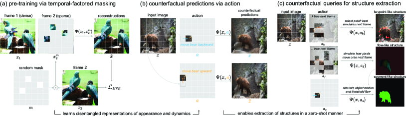
Figure 1: Core concepts of CWM framework (a) Pre-training via temporal-factored masking policy. Given a frame pair input, we train an autoencoder that takes in dense visible patches from the first frame, and only a sparse subset of patches from the second frame as inputs. The model learns to predict the masked patches in second frame. This policy encourages the model to learn disentangled representations of appearance and dynamics. (b) Counterfactual simulation via sampling actions. We can sample an action, specified by one or a few visual patches, to meaningfully control scene dynamics and steer the prediction of the model. (c) Counterfactual queries for structure extraction. The pre-trained model and a set of simple actions constitute the basic ingredients for designing counterfactual queries that extract useful vision structures like keypoints, optical flow, and segmentation in a zero-shot manner.

A contrasting class of approaches avoids the use of structured intermediates by learning to predict raw pixels of future video frames [1, 28, 4, 37, 29, 36, 64, 90]. These approaches are directly applicable to any video input, eliminating the need for annotations. However, learning to predict future frame pixels poses many challenges due to the high-dimensionality of image pixels and the stochasticity of real-world physical dynamics, and the joint learning of scene parsing and prediction can make it more difficult to learn useful scene representations. Previous work [9] indicates that methods with unstructured video prediction tend to underperform compared to methods with structured object-centric representations, and substantially lag behind particle-based methods that have direct access to 3D physical state information.

Beyond task-specific methods for physical dynamics prediction, recent years have seen substantial progress in learning general task-agnostic visual representations [12, 39, 79], following the paradigm shift to foundational models in Natural Language Processing (NLP) [19, 40, 80]. These models leverage large quantities of internet data to learn visual representations that transfer well to downstream vision tasks. Methods including but not limited to DINO [12, 60], masked autoencoder (MAE) [39], and VideoMAE [27, 79, 84] are promising early efforts towards pure vision foundation models. Although they focus on core traditional vision tasks such as image classification, action recognition, and semantic segmentation, their learned representations are potentially useful for dynamics understanding.

Besides learning useful representations, it is promising that vision structures such as segmentations could potentially emerge from this class of vision foundation models [12, 60]. These intermediate structures are useful for dynamics understanding [54, 66, 92, 73]. However, these models are mostly used in the paradigm of transfer learning or finetuning. They cannot be prompted like a Large Language Model (LLM) to extract meaningful structures without model re-training.

One potential workaround for this shortcoming is Vision-Language models [3, 71, 24, 15], which utilize the prompting capabilities of an LLM to answer questions about visual embeddings. However, low-level descriptions of physical dynamics are almost never present in internet-scale vision-text corpora. Thus we cannot expect such models to contain dynamics understanding capabilities.

It would be desirable to have a pure vision foundation model that can be pre-trained on real-world video data and queried visually to extract structures useful for dynamics understanding. In this paper, we use a simple, effective, and scalable framework, called Counterfactual World Modeling (CWM) [10]. Figure 1 illustrates the three core concepts of the CWM framework. First, we pre-train the model with a temporal-factored masking policy for structured masked prediction of video data . Given an input frame pair, we train a masked autoencoder to predict the second frame given only a few patches of it, along with a fully visible first frame [10]. This design is motivated by the observation that the transition between a frame pair can often be explained by a few latent causes (e.g. the motion of an object or a camera pan). As a result, we can simply modify those patches to exert meaningful control on scene dynamics. Second, by virtue of these few embeddings representing latent causes, CWM is capable of generating counterfactual next-frame predictions by taking actions, specified as changes to the corresponding patches. Third, we design unified counterfactual queries for extracting useful vision structures similar to keypoints, optical flows, and segmentations, which are useful for dynamics understanding. We show that the zero-shot readouts of vision structures extracted by CWM attain competitive performance on real-world datasets. Further, we demonstrate that CWM achieves state-of-the-art performance on the challenging Physion benchmark for physical scene understanding.

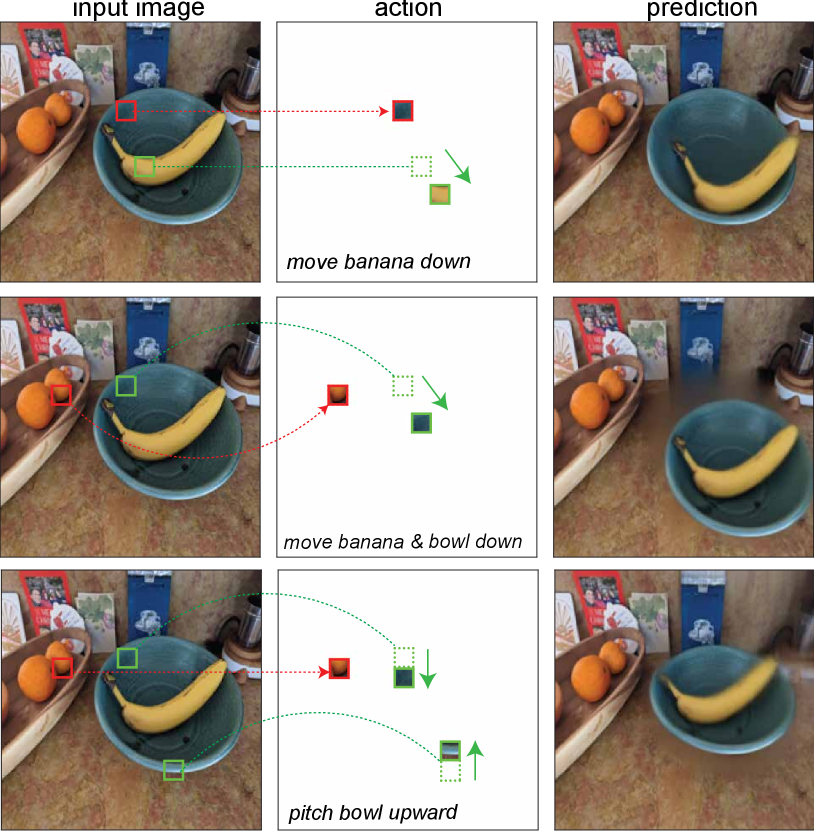
Figure 2: A small number of visual patches exert meaningful control of scene dynamics. Each triplet shows the input image (left), an action constructed from the input image (middle), and the counterfactual prediction of the model (right). Each action is constructed by copying 2-3 patches from the input image. A red patch in the action is copied from the input image into the same location as its source. This prompts the predictor to simulate the appearance of holding an object fixed. A green patch is copied from the input image, but into a different location at an offset from the source location. This simulates the appearance of an apparent object motion.

2 Related Works

Structured dynamics prediction

Researchers in the past decade have made progress in physical dynamics prediction using structured object representations such as segmentations and particle graphs as inputs [8, 54, 44, 7, 77, 70, 55, 2, 73, 92, 66]. The scalability of these approaches on real-world unlabelled data remains limited.

Video prediction

One class of approaches [1, 28, 4, 37, 29, 36, 64, 90] learns general physics understanding through future frame pixel prediction on large unstructured videos of real-world scenes [81]. Recent video diffusion models [82, 49, 41, 18] and transformer-based prediction models [35, 95] have made progress towards more realistic pixel prediction of future video frames.

Self-supervised visual representation learning

from large-scale unlabeled image or video data has drawn increasing attention in recent years. These methods learn to generate visual features that transfer well to downstream vision tasks. One school of works leverages different pretext tasks for pre-training [21, 57, 85, 96, 62, 32]. The recent family of contrastive learning methods models image similarity and dissimilarity between augmented views of an image [89, 58, 38, 17] and different clips of a video [67, 97, 20].

Mask visual modeling

approaches learn effective visual representations via masking and reconstruction of visual tokens. iGPT [16] and ViT [22] pioneer this direction by training transformers on pixel or patch tokens and exploring masked prediction with patches. MAE [39] introduces autoencoding with an asymmetric encoder-decoder architecture and empirically shows that a high masking ratio is crucial for image tasks. VideoMAE [79, 27] extends to the video domains and shows that an even higher masking ratio leads to strong performance for activity recognition tasks.

3 Method

In this section we discuss in generality the three core concepts of CWM (as originally introduced in [10]): (a) pre-training with temporal-factored masked prediction, (b) counterfactual predictions via sampling actions, and (c) counterfactual queries for extracting structures. We will discuss the application of CWM to physical dynamics understanding in Section 4.

3.1 Temporal-factored masked prediction

Masked prediction

Following MAE [39] and VideoMAE [79, 27], we train an encoder-decoder architecture to reconstruct masked observations of video data. Given an input frame pair $x_{1},x_{2}\!\in\!\mathbb{R}^{3\times H\times W}$, we first divide them into non-overlapping spatiotemporal square patches. Then a subset of the patches is masked, and only the remaining visible patches are passed as inputs into the transformer encoder. Finally, the embeded tokens from the encoder and learnable mask tokens, with added positional embedding on all the tokens, are passed as inputs into a shallow decoder to reconstruct the masked patches. The model is trained with the mean squared error (MSE) loss between the reconstructed patches and the original masked patches.

Masking policy

Unlike VideoMAE [79, 27], which randomly samples “tubes” or “cubes” of spatiotemporal patches to be masked, we use a temporal-factored masking policy for video data. This is motivated by the observation that the next frame of a video can be predicted well by simply copying large chunks of the previous frame to nearby locations, especially on short timescales [10]. In other words, information about scene dynamics has a low-dimensional structure even if per-frame appearance does not. This asymmetry between dynamics and appearance can be harnessed with a temporal-factored masking policy [10]. Specifically, given an input frame pair $x_{1},x_{2}\in\mathbb{R}^{3\times H\times W}$, we train a predictor $\Psi$:

$$\Psi(x_{1},x_{2}^{m})=\tilde{x}_{2}$$ (1)

which takes in a fully visible first frame $x_{1}$ and a masked second frame $x_{2}^{m}\in\mathbb{R}^{3\times H\times W}$ with only a random subset of patches visible. The predictor $\Psi$ predicts the masked patches of the second frame, and minimizes the mean squared error (MSE) between reconstructed patches $\tilde{x}_{2}$ and the masked patches in the original $x_{2}$.

When the masking fraction $p\in[0,1]$ of $x_{2}$ is high, the predictor $\Psi$ must complete the second frame given only a few patches of it, along with the fully visible first frame; the only way it can do this is by detecting how objects are moving from the small set of second-frame patches, then applying these transformations to the full objects in the first frame [10]. Thus the predictor trained with this masking policy learns implicitly to use the embeddings of a few patches to represent the latent causes underlying scene dynamics.

3.2 Counterfactual prediction via action

By virtue of patch embeddings representing latent causes, we can modify the content of these patches to steer the next-frame predictions output by the predictor $\Psi$, as illustrated by Figure 2. Formally, given a static input image $x\!\in\!\mathbb{R}^{3\times H\times W}$ during inference, we define action as a sparse frame with a few patches that control the dynamics of the scene, denoted by $a\!\in\!\mathbb{R}^{3\times H\times W}$. The action will be passed as an input to the predictor along with the input image to steer the output of the predictor:

$$\Psi(x,a)=\tilde{x}$$ (2)

The alternative prediction $\tilde{x}$ given an action is a counterfactual prediction [10]. Next, we define an operator for sampling actions $a$ that meaningfully controls the dynamics of the scenes.

Algorithm 1 Sampling actions

1:function sample($x$, $p$, $n$, $r$)

2:    $a\leftarrow\textsc{zero\_like}(x)$ $\triangleright$ initialize an empty action

3:    $\epsilon_{1},\epsilon_{2}\sim\textsc{Uniform}(-r,r)$ $\triangleright$ sample a location offset

4:    for $1$ to $n$ do $\triangleright$ iterate to sample n patches

5:       $(i,j)\sim\textsc{multinomial}(p,1)$ $\triangleright$ sample a patch location

6:       $a[i\!+\!\epsilon_{1},j\!+\!\epsilon_{2}]\leftarrow x[i,j]$ $\triangleright$ copy the patch content

7:    end for

8:    return $a$ $\triangleright$ $a\!\in\!\mathbb{R}^{3\times H\times W}$

9:end function

Sampling operator

Algorithm 1 describes the operator for sampling actions. Given an input RGB image $x$, the sampling operator constructs an action $a\!\in\!\mathbb{R}^{3\times H\times W}$, which has $n$ visible patches. Each visible patch is copied from a source location in the input image, with each source location randomly sampled from a spatial probability distribution $p\in\mathbb{R}^{H\times W}$. In addition, each visible patch can be optionally copied to a new patch location with a random offset within radius $r$ from the source location. This will create a motion counterfactual that simulates the appearance of moving the object associated with the patch.

3.3 Counterfactual queries for structure extraction

With a predictor and an operator for sampling actions, we can compose these two ingredients into programs for extracting vision structures, including keypoints, optical flows, and segmentation.

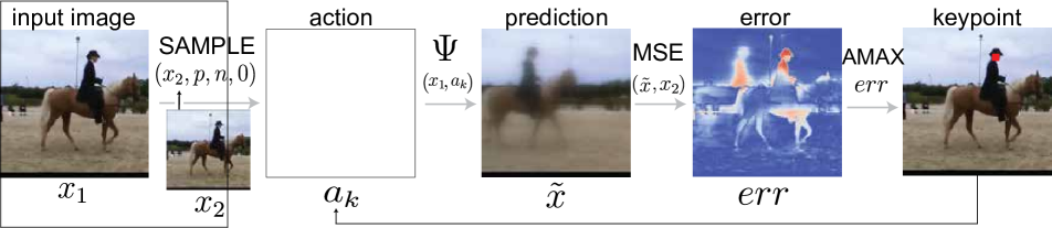
Algorithm Extract keypoints

1:procedure extract_keypoint($x_{1},x_{2}$)

2:    $K\leftarrow\varnothing$ $\triangleright$ K represents a set of keypoints

3:    $a\leftarrow\textsc{zeros\_like}(x_{1})$ $\triangleright$ initialize action as empty frame

4:    for $1$ to $iter$ do $\triangleright$ each iteration adds 1 keypoint

5:       $\tilde{x}\leftarrow\Psi(x_{1},a)$ $\triangleright$ predicting next frame

6:       $err\leftarrow\textsc{mse}(\tilde{x},x_{2})$ $\triangleright$ compute reconstruction error

7:       $(i,j)\leftarrow\textsc{argmax\_2d}(err)$ $\triangleright$ select (i,j) with max error

8:       $K\leftarrow K\cup(i,j)$ $\triangleright$ add to the set of keypoints

9:       $p\leftarrow\textsc{zeros\_like}(x)$ $\triangleright$ initialize a probability map

10:       $p[i,j]\leftarrow 1$ $\triangleright$ 1 at the keypoint location

11:       $a\leftarrow\textsc{Sample}(x_{2},p,1,0)$ $\triangleright$ equivalent to $a[i,j]\leftarrow x_{2}[i,j]$

12:    end for

13:    return $K$ $\triangleright$ list of keypoint locations

14:end procedure

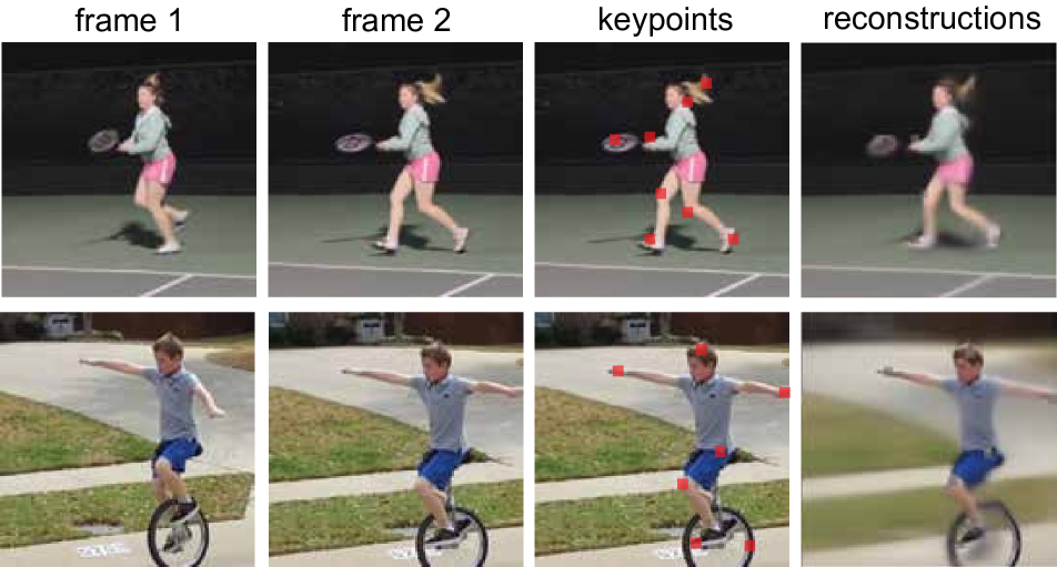
Figure 3: Counterfactual query for keypoints The first panel and the algorithm describe an iterative procedures for extracting keypoints given an frame pair $x_{1},x_{2}$ as input. Starting with an action with no visible patches, the algorithm selects a location with maximum reconstruction error as the keypoint. The keypoint patch is then added to the action in the next iteration, and this process iterates to extract multiple keypoints $K$. The last panel shows that with only 8 keypoints (1% of the totalpatches), the predictor is capable of predicting the next frame and capturing dynamics well.

Keypoints

are local features of a scene that capture more information than other features [53, 52, 10]. In our approach, keypoints are naturally defined as those tokens that, when made visible to the predictor $\Psi$, yield lowest reconstruction error on the rest of the scene [10]. Keypoints turn out to be good loci for exerting counterfactual control. Intuitively, this is because they are the few visual tokens most able to reduce uncertainty and yield a concrete prediction about many other tokens [10]. Figure 3 describes an iterative procedure for constructing keypoints. Given a frame pair $x_{1},x_{2}$, we start from a null action with no visible patches and iteratively add visual patches one-by-one greedily to reduce the reconstruction error of $x_{2}$ given $x_{1}$ and the action as inputs. At each iteration, we choose the location with maximum reconstruction error as the keypoint and add its corresponding patch into action. These keypoint patches are most able to reduce uncertainty of the scenes.

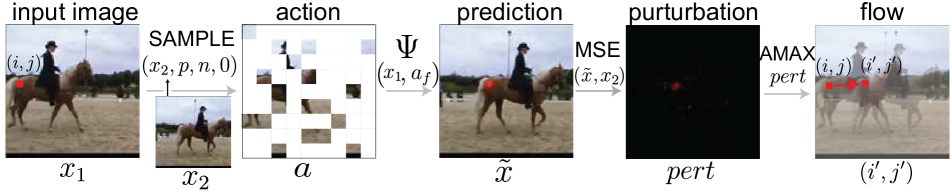
Algorithm Extract optical flow at location $(i,j)$

1:procedure prompt_optical_flow($x_{1}$, $x_{2}$)

2:    $\bar{X}\leftarrow\varnothing$ $\triangleright$ init a list for predictions

3:    $p\leftarrow\textsc{ones\_like}(x_{2})$ $\triangleright$ uniform sampling distribution

4:    $p\leftarrow p_{k}/\sum_{k}p_{k}$ $\triangleright$ normalization

5:    for $1$ to $iter$ do $\triangleright$ loop over mask samples

6:       $a=\textsc{sample}(x_{2},p,n,0)$ $\triangleright$ sample actions with $x_{2}$ patches

7:       $\bar{x}_{1}\leftarrow x_{1}+\delta_{i}$ $\triangleright$ perturb frame 1

8:       $\bar{X}\leftarrow\bar{X}\oplus\Psi(\bar{x}_{1},a)$ $\triangleright$ store the perturbed prediction

9:    end for

10:    $\bar{\delta}\leftarrow|\textsc{mean}({\bar{X}})-x_{2}|$ $\triangleright$ compute perturbation response

11:    $i^{\prime},j^{\prime}\leftarrow\textsc{argmax\_2d}(\bar{\delta})$ $\triangleright$ locate the perturbation in $x_{2}$

12:    $flow\leftarrow(i^{\prime}\!-\!i,j^{\prime}\!-\!j)$ $\triangleright$ flow is the displacement

13:    return $flow$ $\triangleright$ flow for location $i$

14:end procedure

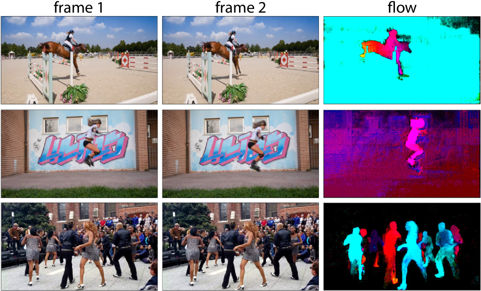
Figure 4: Counterfactual query for flow. The first panel and algorithm describe a procedure for extracting optical flow at location $(i,j)$. Flow is obtained by perturbing the first frame of the image at a given location, propagating the perturbation through the CWM, and comparing the perturbed response to the original second frame. Qualitative examples of optical flow on the DAVIS dataset [65] are shown here.

Optical flow

Flow-like structure can be queried by adding a small “tracer” to the first frame at position $(i,j)$ and localizing the response of the perturbation in the counterfactual prediction of the next frame [10]. The procedure is described in Figure 4. Given a frame pair $x_{1},x_{2}$ and a pixel location $(i,j)$, we add a small perturbation to the pixel and construct an action $a$ with randomly selected patches from $x_{2}$ to specify the motion between frame pair. In the predicted next frame $\tilde{x}$ output by $\Psi$, the perturbation is propagated to the corresponding location according to the scene motion. Taking the difference between $\tilde{x}$ and $x_{2}$ gives the perturbation responses over the entire image, and the location with the highest response is set as the corresponding pixel location $(i^{\prime},j^{\prime})$ in $x_{2}$. Flow is calculated as the spatial displacement between $(i,j)$ and $(i^{\prime},j^{\prime})$.

Segmentation

Our querying procedure for segmentation is inspired by the notion of Spelke object in infant object recognition: babies typically treat things that move together as a single object [74]. The CWM model segments objects by sampling counterfactual motion at a pixel location, predicting the next frame, and grouping together parts of the image that move similarly to the counterfactual motion.

Figure 5 describes an iterative procedure for generating motion counterfactual and extracting segments associated with a pixel location $(i,j)$. Given a single input image $x$, we instantiate an action by creating a new frame that is mostly blank, but in which the content of the patch at location $(i,j)$ of the input image is copied to a new location $(i\!+\!\epsilon_{1},j\!+\!\epsilon_{2})$, where $\epsilon_{1},\epsilon_{2}$ are location offsets sampled within a radius $r\!>\!0$. With a pre-trained predictor, moving a single patch causes the whole object to move in the predicted frame [10]. We extract the flow between the input and predicted frame, and threshold it to obtain a segment. To further refine the segments, we repeat this procedure by iteratively adding more patches within the segment region into the action, where the number of iterations is set as 3.

To automatically discover multiple objects in a single image, we choose actions at pixel locations based on a sampling probability distribution $p$, which has high probability at pixel locations belonging to Spelke objects and low otherwise. Once a segment is discovered, we mask out the probability distribution values using the segments and repeat the process to discover the next object. We discuss more details about computing the sampling distribution in the supplementary materials.

3.4 Implementation details

CWM uses the standard ViT-B and ViT-L architectures with a patch size of 8, which allows structure extraction at a higher resolution. We pre-train CWM on the Kinetics-400 dataset [43], without requiring any specialized sparse operations or temporal downsampling. While the discussion about CWM thus far assumes a frame pair as input, it can be easily generalized to take in multiple frames as input. Our default setting is sampling 3 video frames 150ms apart on the Kinetics-400 dataset. It takes approximately 6 days to train 3200 epochs on a TPU v4-256 pod.

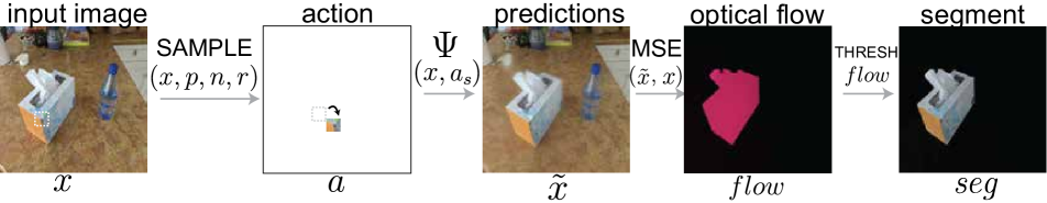
Algorithm Extract Spelke object segment at location $(i,j)$

1:procedure prompt_segment($x$)

2:    $p\leftarrow\textsc{zeros\_like}(x)$ $\triangleright$ init probability distribution

3:    $p[i,j]\leftarrow 1$ $\triangleright$ set as 1 in the queried location

4:    $n\leftarrow 1$ $\triangleright$ start with sampling 1 patch in the action

5:    for $1$ to $iter$ do

6:       $a\leftarrow\textsc{Sample}(x,p,n,r)$ $\triangleright$ sample counterfaction motion

7:       $\tilde{x}\leftarrow\Psi(x,a)$ $\triangleright$ predict next frame

8:       $flow\leftarrow\textsc{Flow}(x,\tilde{x})$ $\triangleright$ compute flow between $x$ and $\tilde{x}$

9:       $seg\leftarrow\textsc{norm}(flow)>0$ $\triangleright$ threshold flow magnitude

10:       $p\leftarrow p+seg$ $\triangleright$ update p for next iteration

11:       $p\leftarrow p_{k}/\sum_{k}p_{k}$ $\triangleright$ normalization

12:       $n\leftarrow n+1$ $\triangleright$ sample more patches in next iteration

13:    end for

14:    return $seg$ $\triangleright$ binary segmentation map of shape $H\!\times\!W$

15:end procedure

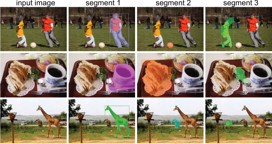
Figure 5: Counterfactual query for extracting Spelke object segment. The first panel and the algorithm describe an iterative procedure for extract segmentation at location $(i,j)$ of a static image $x$. CWM segments objects by sampling a counterfactual motion at the pixel location, predicting the next frame, and grouping together parts of the image that move similarly to the counterfactual motion. The last panel shows qualitative segmentation results on COCO [46] images. Three segmentation masks are extracted and shown for each image.

4 Experiments

In this section, we first evaluate CWM’s ability to extract zero-shot visual structures such as optical flow and Spelke object segments on real-world datasets (Section 4.1). Second, we investigate whether these structures help improve performance on downstream physical dynamics understanding tasks (Section 4.2). Last, we perform ablations studies on CWM design with the ViT-B architecture on Kinetics-400 [43] dataset (Section 4.3).

4.1 Visual structure extraction

Optical flow

We evaluate the quality of optical flows using the SPRING benchmark [50], which is a simulated movie dataset with high-resolution videos and ground-truth optical flows. We compare CWM to previous supervised flow estimation methods including RAFT [78], PWCNet [76] and SpyNet [68]. We report the average endpoint error (epe) metric [61] in Table 1(a). Although CWM is not trained with the specific objective of learning optical flow, the extracted flow-like structures are meaningful, as illustrated in Figure 4. While CWM, trained in an unsupervised manner is inferior to RAFT and PWCNet trained with ground-truth supervision, it still achieves comparable performance to the prior supervised method SpyNet. We include qualitative comparisons to these methods and additional implementation details in the supplementary.

Spelke object segmentation

We extract zero-shot segmentations on images from COCO train2017 [45] using counterfactual queries. Although Spelke object are segment-like structures, the definition of Spelke objects is not exactly aligned with the definition of instance segmentations in the COCO datasets, therefore we are not optimizing our querying procedure for the COCO evaluation metrics. We follow the same procedures in CutLER [87] to learn a detector using the popular Cascade Mask R-CNN [11] on these coarse masks in a self-supervised manner while being robust to objects missed by the query. We compare CWM with TokenCut [88], FreeSOLO [86] and CutLER [87]. These methods extract segment-like structures from pre-trained models and learn a detector using pseudo ground-truth masks as self-supervision. We train CutLER on COCO training images for a fair comparison.

Method	epe $\downarrow$
RAFT [78]	1.476
PWCNet [76]	2.288
SPyNet [68]	4.162
CWM	4.981

((a)) Flow Results on SPRING

Method	$\text{AP}^{\text{box}}$ $\uparrow$	$\text{AP}^{\text{mask}}$ $\uparrow$
TokenCut [88]	3.0	2.4
FreeSOLO [86]	4.2	4.3
CutLER [87]	10.8	8.42
CWM	10.0	8.20

((b)) Detection and segmentation on COCO val2017

Table 1: To assess the quality of CWM’s zero shot vision structures, we show quantitative comparisons to baseline methods in (a) optical flow estimation on the SPRING benchmark and b) object detection and segmentation on COCO val2017.

Table 1(b) shows the quantitative performance of CWM and the baseline methods in unsupervised class-agnostic object detection and segmentation on COCO [45] validation set. CWM outperforms prior methods TokenCut [88], and FreeSOLO [86] significantly and attains similar performance to the current state-of-the-art, CutLER [87].

4.2 Physical Dynamics Understanding

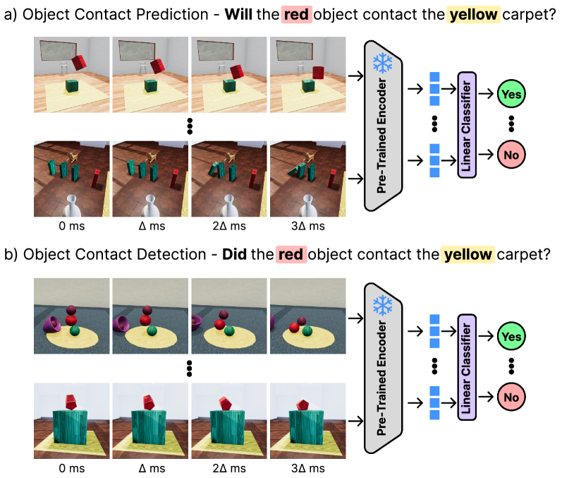
Figure 6: Physion v1.5 evaluation protocol. We evaluate on two physical dynamics understanding tasks – (a) Object contact prediction where the model is asked to predict contact events in the future and (b) Object contact detection where the model is asked to reason about contact events that occur in the observed video stimulus. The objects of interest for which we want to ask the contact question are rendered with red and yellow texture to cue the model.

Having demonstrated CWM can use patch embeddings to meaingingfully control scene dynamics and query different vision structures, we study the usefulness of these embeddings and the extracted structures for dynamics understanding. We adopt a similar evaluation procedures as the Physion [9] benchmark, which assesses physical scene understanding of pre-trained models by how well those models predict whether two objects will collide in the future given a context video.

Physion benchmark

consists of realistic simulations of diverse physical scenarios where objects are manipulated in a variety of configurations to test different types of physical reasoning such as stability, rolling motion, containment, object linkage, etc. We use the latest version of Physion [9], referred to as Physion v1.5, which has improved rendering quality and more physically plausible simulations. In the ideal scenario, we would evaluate CWM on a real-world physics-understanding benchmark, but such benchmarks are not available. Despite being a synthetic dataset, Physion serves as a strong out-of-distribution generalization test for vision foundation models trained on real world data. Physion is also more challenging as it contains diverse physical phenomena, object dynamics and realistic 3D simulations. This makes it a preferable choice when compared to other benchmarks such as ShapeStacks [34] and IntPhys [69] which contain very limited object dynamics, or Phyre [5] which only operates in 2D environments. The benchmark consists of two tasks: (a) Object contact prediction (OCP), which tests the model’s ability to predict whether two objects will contact at some point in the future given a context video, and (b) Object contact detection (OCD) which tests the model’s ability to detect if two objects have already come into contact in the observed video. For both tasks, the two objects of interest are rendered with red and yellow texture to cue the model. Figure 6 shows example stimuli for the two tasks.

Evaluation protocol

We follow the three-step evaluation protocol of the Physion benchmark [9]. First, we extract features from the last layer of a frozen pre-trained encoder on a training set of 5608 videos for OCP and OCD tasks, respectively. For image-based methods, features are extracted from 4 frames that are 150 ms apart. For video-based methods, the input frames are fed to the model at the specific frame rate used during their training. Second, the extracted features are used to train a logistic regression model to predict the contact label for the given video stimulus. We search for the optimal regularization strength by validating over 5 training-set folds. Lastly, the trained classifier is evaluated on a test set of 1035 videos, sampled equally across different physical scenarios.

Baseline methods

We compare CWM with four classes of baseline approaches: (a) video prediction models including MCVD [82], R3M [56], FitVid [4], and TECO [91], (b) self-supervised representation learning methods on images including DINO [12], DINOv2 [60], and MAE [39], (c) self-supervised representation learning methods on videos including VideoMAE [79] and VideoMAEv2 [84], and lastly (d) vision-language model like GPT4-V [59].

method	pre-train data	arch	params	OCP $\uparrow$	OCD $\uparrow$
video prediction models
MCVD [82]	K400+Ego4D	UNet	251 M	63.4	80.8
R3M [56]	K400+Ego4D	Res50	38 M	67.6	78.1
FitVid [4]	K400+Ego4D	VAE	303 M	64.3	59.5
TECO [91]	K600	vq-gan	160 M	69.3	80.9
self-supervised image representation models
DINO [12]	IN-1K	ViT-B	86M	72.1	85.4
DINOv2 [60]	LVD-142M	ViT-B	86 M	72.2	87.1
DINOv2 [60]	LVD-142M	ViT-L	304 M	72.2	85.5
DINOv2 [60]	LVD-142M	ViT-g	1.1 B	72.7	84.6
MAE [39]	IN-1K	ViT-B	86 M	72.6	81.6
MAE [39]	IN-1K	ViT-L	304 M	71.6	82.3
MAE [39]	IN-1K	ViT-H	632 M	73.3	80.8
MAE [39]	IN-4.5M	ViT-B	86 M	72.1	81.7
MAE [39]	IN-4.5M	ViT-L	304 M	72.6	81.9
self-supervised video representation models
VMAE [79]	K400	ViT-B	86 M	72.1	85.7
VMAE [79]	K400	ViT-L	304 M	73.6	86.1
VMAE [79]	K400	ViT-H	632 M	73.5	87.5
VMAEv2 [84]	U-Hybrid	ViT-g	1.1B	72.2	85.0
vision-language models
GPT4-V [59]	-	-	-	52.9	54.7
CWM-feat	K400	ViT-B	86 M	73.6	89.1
CWM-feat	K400	ViT-L	304 M	74.6	88.6
CWM	K400	ViT-B	86 M	75.9	89.1
CWM	K400	ViT-L	304 M	76.1	88.7

Table 2: Physion v1.5 results. We compare CWM to four classes of baseline methods across different architectures on the OCP and OCD tasks. Even without extracted structures, CWM-feat with backbone features alone achieves state-of-the-art results on both OCP and OCD accuracy. With both features and extracted structures, CWM further improves the OCP accuracy.

Results

In Table 2 we report results on the two Physion tasks for both CWM with ViT-B and ViT-L architectures and other baseline methods discussed above. We evaluate CWM in two settings: CWM-feat only uses the embeddings from the last layer of the pre-trained encoder as the input to the linear classifier, and CWM uses both features and extracted vision structures. We find that even without extracted structures, CWM-feat with ViT-B achieves state-of-the-art results on both OCP and OCD metrics. It is interesting to note that CWM outperforms baseline methods such as DINOv2 ViT-g and MAE ViT-H which have 13 and 7 times more parameters. This shows that CWM is a more effective and efficient learner of physical scene dynamics. We also observe that CWM, when scaled up to the ViT-L architecture, achieves superior performance on the OCP task. With the extracted structures, the OCP improves from 73.6% to 75.9% in ViT-B architecture and 74.6% to 76.1% in ViT-L architecture. This shows that the extracted vision structures are useful for dynamics understanding.

We find that video prediction models perform poorly especially on the harder OCP task. Self-supervised methods on the other hand, are better in terms of both OCP and OCD metrics, but they saturate around 72% and 87% respectively with the ViT-B architecture.

We also evaluate GPT4-V [59] on Physion v1.5 tasks by providing it with a single composite image with a sequence of four video frames sampled at a gap of 150ms. The model is prompted with questions similar to those in Figure 6 (see supplementary for more details about the specific prompts used). We find GPT4-V scores nearly at chance on OCP and slightly above chance on OCD, which highlights a considerable limitation in the ability of large-scale VLMs to understand physical scene dynamics.

4.3 Ablation studies

We ablate the CWM design with the default backbone of ViT-B. Each ablated model is trained for 800 epochs on the Kinetics-400 dataset. Although optimal performance is not reached at 800 epochs, reasonable results are achieved, allowing fair and efficient ablations.

Mask ratio

Table 3(a) shows the influence of the target frame mask ratio. We observe that a high ratio during model training achieves good performance on both the OCP and OCD tasks. The optimal mask ratio for CWM is higher than the mask ratio used in MAE [39] which is 75%. This trend aligns with our aforementioned hypothesis that the dynamics between frame pairs at a short timescale has a low-dimensional causal structure, which can be concentrated into a small number of tokens.

Mask ratio	OCP $\uparrow$	OCD $\uparrow$
0.85	73.4	87.3
0.90	73.9	87.1
0.95	73.4	87.9
0.99	72.6	85.4

((a)) Mask ratio

#frames	OCP $\uparrow$	OCD $\uparrow$
1	70.6	80.8
2	73.9	87.1
4	68.7	77.7

((b)) Context length

Patch size	OCP $\uparrow$	OCD $\uparrow$
16	73.5	87.3
8	73.6	87.1

((c)) Patch size

epochs	OCP $\uparrow$	OCD $\uparrow$
800	73.6	87.1
3200	73.6	89.1

((d)) Training schedule

Input to the linear classifier				Metric
Feat.	Keypt.	Flow	Segments	OCP $\uparrow$	OCD $\uparrow$
✓	✗	✗	✗	73.6	89.1
✓	✓	✗	✗	74.4	89.1
✓	✓	✓	✗	75.5	88.5
✓	✓	✓	✓	75.9	89.1

((e)) Utility of different vision structures

Table 3: CWM ablation studies. In this set of tables, we study the effect of different architectural choices, training conditions and demonstrate the utility of different vision structures extracted from CWM towards improving performance on Physion tasks. Refer Section 4.3 for a detailed description of the results.

Context length

We compare the performance of CWM with different numbers of context frames in Table 3(b). CWM with 2 context frames during pre-training performs better as compared to using 1 context frame. However, including 4 context frames degrades the performance.

Patch size

We find that the choice of patch size has relatively small influence on the OCP and OCD accuracy (See Table 3(c)). We choose the default patch size to be 8 since it enables CWM to output higher resolution segmentation and optical flow maps when prompted.

Training schedule

A longer training schedule (3200 epochs) has a relatively small influence on the OCP accuracy, but it has noticeable improvement on the OCD accuracy. We report these results in Table 3(d).

Vision structures

Table 3(e) studies the importance of different visual structures in the performance of OCP and OCD using ViT-B architecture. We find that incorporating vision structures from CWM improves performance. First, adding patch features at keypoint locations improves the OCP scores from 73.6% to 74.4%. Second, enriching these patch features with optical flow patches computed at keypoint locations further improve the OCP scores to 75.5%. Finally, including spelke object segments achieves a score of 75.9%, demonstrating the cumulative impact of successive additions.

5 Discussion and Conclusion

In this work, we show how Counterfactual World Modeling, an approach for building pure vision foundation models, can be useful for dynamics understanding. CWM utilizes a temporal-factored masked prediction objective for pre-training, which encourages the model to learn disentangled visual and motion representations over a short video clip. CWM supports counterfactual prediction, which enables a spectrum of queries for extracting useful vision structures such as keypoints, optical flows, and Spelke object segments from the model in a zero-shot manner. This serves as a general framework for pre-training on internet-scale video datasets and visually querying the pre-trained model to extract structures useful for dynamics understanding.

Currently the model is only capable of predicting future frames at short timescale around 450 ms. While this is enough for extracting useful vision structures, future versions could extend to longer time scales in order to solve meaningful predictive control tasks.

In future work, the CWM framework could be extended to query 2.5D structures such as depth and lifting multiview information to 3D structures. Additionally, automatic query discovery systems could identify useful structures without human design. CWM could also serve as a powerful tokenization scheme for modeling longer-range dynamics prediction via both the extracted structures and embeddings that represents latent causes of the scene dynamics. The capability of long-range prediction coupled with the counterfactual querying mechanism could be a promising tool for applications that involve model-predictive control and planning such as robotics and autonomous driving.

Acknowledgements

This work was supported by the following awards: To D.L.K.Y.: Simons Foundation grant 543061, National Science Foundation CAREER grant 1844724, Office of Naval Research grant S5122, ONR MURI 00010802 and ONR MURI S5847. We also thank the Google TPU Research Cloud team for computing support.

1

Supplementary Material

1 CWM pre-training

In this section, we describe architecture details and default pre-taining settings of the predictor $\Psi$ in the CWM framework.

1.1 Architecture details

Figure 7 provides an overview of the predictor architecture. The input video is first divided into non-overlapping spatiotemporal patches of size $8\times 8$. Then a subset of patches is masked, and only the remaining visible patches are passed as inputs into the transformer encoder. We follow the standard ViT architecture. Following MAE [39], each transformer block in the ViT consists of a multi-head self-attention block and an MLP block, both having LayerNorm (LN). The CWM encoder and decoder have different widths, which are matched by a linear projection after the encoder [39]. Finally, the embedded tokens from the encoder and learnable mask tokens are passed as inputs into a shallow decoder to reconstruct the masked patches. Each spatiotemporal patch has a unique sine-cosine positional embedding. Position embeddings are added to both the encoder and decoder inputs. CWM does not use relative position or layer scaling [6, 39].

1.2 Default settings

We show the default pre-training settings in Table 4. CWM does not use color jittering, drop path, or gradient clip. Following ViT’s official code, xavier uniform is used to initialize all Transformer blocks. Learnable masked token is initialized as a zero tensor. Following MAE, we use the linear lr scaling rule: $lr=base\_lr\times batch\_size\,/\,256$ [39].

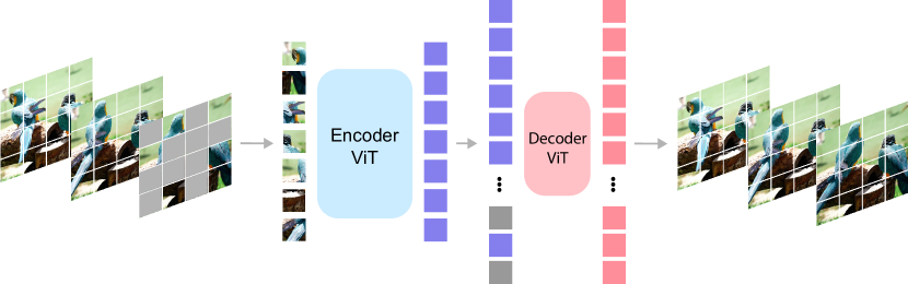
Figure 7: Architecture of predictor $\Psi$ in the CWM framework

config	value
optimizer	AdamW [48]
base learning rate	1.5e-4
weight decay	0.05
optimizer momentum	$\beta_{1},\beta_{2}=0.9,0.95$ [16]
accumulative batch size	4096
learning rate schedule	cosine decay [47]
warmup epochs [33]	40
total epochs	3200
flip augmentation	no
augmentation	MultiScaleCrop [83]

Table 4: Default pre-training setting of CWM

2 Mathematical formulation of vision structure extraction

In this section we formally define the operations used to extract keypoints, optical flow, and Spelke object segments. For clarity, this section is largely a recapitulation of the contents in the paper [10], but it is presented here for readers’ convenience. We refer the readers to Section 2 and 3 of the paper [10] for further details.

2.1 Keypoints

In Section 3.3 of the main text we define a query for extracting keypoints from a given input frame pair, as originally described in [10]. Here we formally define that procedure. Let $\Psi$ be the CWM predictor. Suppose we are given an input frame pair $x_{1},x_{2}$, an initial patch index set $p_{0}$, and an integer $k$. The $k$-subsequent keypoint set for $x_{2}$ from $p_{0}$ is

$$K(x_{1},x_{2},p_{0},k)=\operatorname*{arg\,min}_{\{p\,\subset\,\mathcal{I}-p_{0}\,|\,|p|=k\}}\mathcal{L}(\Psi(x_{1},{x_{2}}_{p_{0}\cup p}),x_{2})$$

where ${x_{2}}_{p_{0}\cup p}$ denotes the patches of $x_{2}$ at the patch index set $\,p_{0}\cup p$ [10]. Ideally it would be possible to efficiently compute $K(x_{1},x_{2},p_{0},k)$ directly for large $k$. However, this is in general an intractable optimization problem. Instead, it is substantially more efficient (though still rather inefficient in absolute terms) to take a greedy approach by finding one keypoint at a time and iterating, e.g. defining

$$k_{i}=k_{i-1}\cup K(x_{1},x_{2},k_{i-1},1),\quad\text{where }k_{0}=\varnothing.$$

2.2 Flow as derivatives

Section 3.3 also describes the counterfactual query for extracting optical flow at a pixel location $i$, as originally described in [10]. The querying procedure starts by injecting a perturbation $\delta$ at location $i$ of the first frame $x_{1}$, and then inspects how the perturbation is propagated onto the next frame $x_{2}$ using the predictor $\Psi$. This procedure has one potential failure mode: the perturbed frame $x_{1}^{i}$ could be out of distribution for $\Psi$. This could happen when the perturbation is either too large so that it looks “fake” rather than like a piece of the surface it is placed on, or too small so that it cannot be detected and moved accurately. This is naturally addressed by considering $\Psi$’s infinitesimal responses to infinitesimal perturbations – which are exactly the derivative of the prediction model [10]:

Normalized Perturbation Response at i

$$=\lim_{\delta\rightarrow 0}\frac{|\tilde{x}^{i}_{2}-x_{2}|}{|x^{i}_{1}-x_{1}|}$$

$$=\nabla_{x}\Psi\bigg{|}_{i}$$ (3)

To simultaneously estimate optical flow at all locations in an $H\times W$ frame pair, we can compute the Jacobian of $\Psi$. This is a four-tensor $\mathcal{J}\Psi$ of shape $H\times W\times H\times W$, which assigns to element $(i,j,k,l)$ the predictor’s change in output at location $(k,l)$ in the second frame due to an infinitessimal change at location $(i,j)$ in the first frame. Applying this derivative implementation to the algorithm above,

$$\textbf{flow}(k,l)=\begin{cases}\text{undefined},&\text{if }\mathcal{J}\Psi(i^{\prime},j^{\prime},k,l)|\ll 1\\ (k,l)-(i^{\prime},j^{\prime}),&\text{otherwise}\\ \end{cases}$$ (4)

where $(i^{\prime},j^{\prime})=\operatorname*{arg\,max}_{i,j}\mathcal{J}\Psi(i,j,k,l)$. Note that this method detects disocclusion at the location where flow is undefined. This method does not detect occlusion, since no perturbation at any location in the first frame will cause a response at a point that becomes disoccluded in the second frame.

Because it is a tensorial operation, the derivative formulation of the counterfactual enables a more efficient parallel computation for flow than serial finite perturbations, implemented practically using Jacobian-vector products available in autograd packages such as PyTorch or Jax.

2.3 Spelke affinities as derivatives

As described in [10], while it is impossible to pin down general definitions of “object” or “segmentation”, an early developmental shift in perception suggests the practically useful notion of a Spelke object. Work by cognitive scientist Elizabeth Spelke and her colleagues revealed that babies begin life grouping separated visual elements into objects only when they are moving in concert; it is not until they are almost a year old that babies expect, for example, two stationary toys resting on each other to be independently movable [74]. We therefore define a Spelke object as a collection of physical stuff that moves together during commonplace physical interactions [10]. This includes common physical objects like cell phones, wallets, coffee cups, dogs, people, and cars, as well as complex novel objects from semantically unnamed categories that nonetheless can be seen to move coherently.

Inspired by the notion of Spelke object, we relax the definition of “object” or “segmentation” to pairwise affinities between scene elements, which is high for two elements that often move together and low otherwise. It is the set of possible affinities – that is, how often would two elements move together across a wide variety of dynamics – that supports a good representation of how objects should be grouped and how they can behave.

This relaxation of segments to pairwise affinities allows the above algorithm to be interpreted as another derivative of $\Psi$ (combined with the optical flow estimator.) We define the Spelke affinity between two points $i$ and $j$ to be the response in the flow estimate at $j$ given a counterfactual change in the flow estimate at $i$. For any input frame pair $(x,y)$ (including frame pairs for which $x=y$, i.e. static images), in the infinitesimal limit of the motion counterfactual size, we can write the Spelke affinity between $i$ and $j$ as $\partial_{y_{i}}\textbf{Flow}(x,y)[j]$, or in tensorial form:

$$\textbf{SpelkeAffinity}[x]=\nabla_{y}\textbf{Flow}[x,y].$$ (5)

Even when objects can undergo complex motion, such that pairs of points sometimes move together and sometimes do not, partial or complete Spelke affinities can be converted to (binarized) estimated segments via grouping operation such as Kaleidoscopic Propagation introduced in [14]. Besides providing an efficient method for segmenting Spelke objects, this derivative construction conceptually unifies segmentation with optical flow estimation – illustrating that two apparently distinct computer vision tasks emerge, zero-shot, from the same unsupervised model.

3 Structure extraction details and results

In this section, we discuss implementation details of the counterfactual queries for extracting keypoints, optical flow, and segmentations. We also provide more visualizations of each structure extracted by CWM.

3.1 Keypoint

Implementation details

CWM queries keypoints iteratively, starting with an action initialized as an initial empty mask and adding visible tokens one-by-one. Note that, whereas the counterfactual queries for optical flow and segmentation involve perturbing the visual input to the predictor $\Psi$, keypoints arise by varying the prediction model’s input mask.

At each iteration, we compute the Mean-Squared-Error (MSE) between the next-frame predictions of $\Psi$ and the ground-truth next frame. We sort the MSE and select the top $k$ locations as candidate keypoints. $k$ is set as 4 by default. For each candidate keypoint, we add its patch content to the action and re-compute the MSE between the updated predictions of $\Psi$ and the ground-truth next frame. The candidate keypoint with the minimum MSE error, or equivalently maximum error reduction, is selected as the keypoint output at that iteration. The selected keypoint is added to the action and we repeat the procedures above to compute the location of the next keypoint.

Qualitative results

Figure 8 shows more qualitative results of the keypoints extracted on DAVIS 2016 [63] and Bridge dataset [25]. We extract 5 keypoints for each example. Our procedure extracts dynamical RGB keypoints in the input frame pairs.

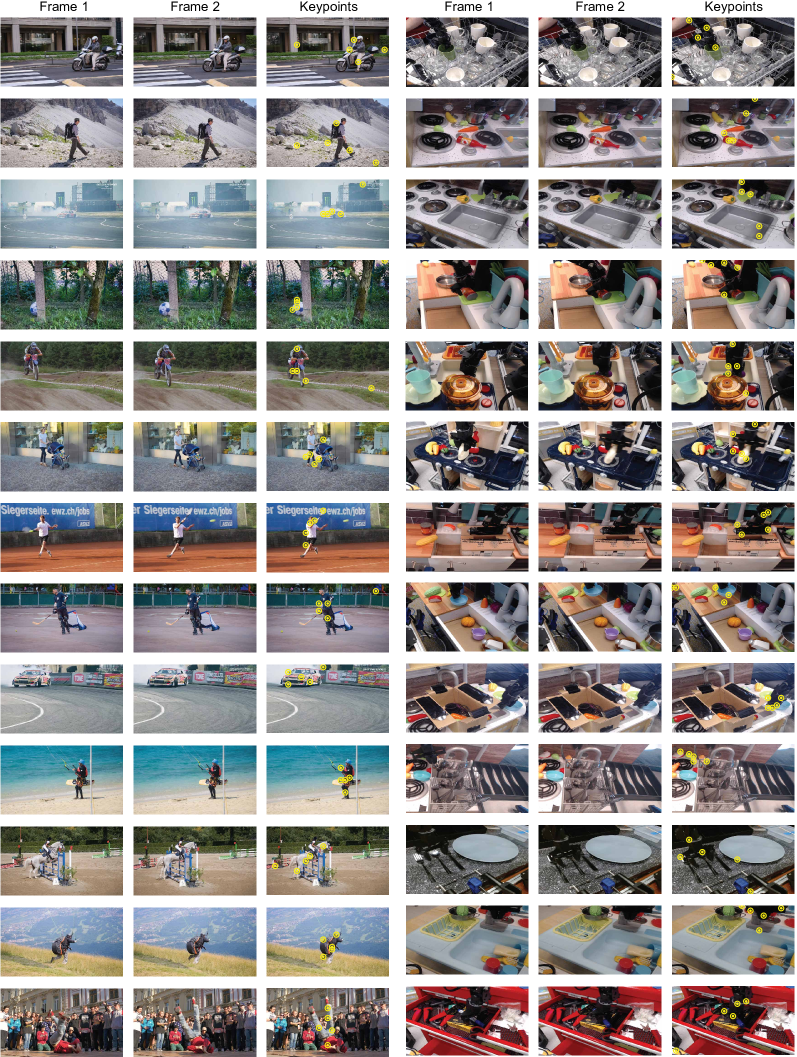
Figure 8: Keypoints extracted by CWM. We extract 5 keypoints for each example on DAVIS 2016 (left) and Brige dataset (right).

3.2 Flow

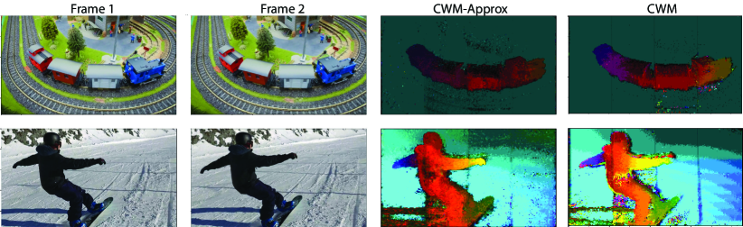
Figure 9: Comparison between the pertubation method and cosine approximation We compare the full perturbation-based optical flow extraction algorithm introduced in the main paper against the cosine-similarity approximation given in Algorithm 5. The fidelity of the approximation method is very close to the complete flow estimate, while benefiting from much lower computational complexity.

Efficient Flow Calculations

The method of extracting optical flow outlined in the main text is designed to extract precise optical flows but comes at a cost of computational expense – the flows are extracted by querying the predictor $\Psi$ multiple times at each pixel location. To address this computational challenge, we propose an approximation to the perturbation method that is faster and attains similar flow performance. The approximation method is described in algorithm 5.

The perturbation method computes flow for each pixel by perturbing it and tracking how the perturbation propagates onto the next frame via multiple forward passes of $\Psi$. This process has to be repeated for every pixel to compute the full flow map, which is computationally slow.

The proposed approximation tracks motion via the cosine similarity of the intermediate embeddings from the ViT encoder, which requires only a few forward passes of the encoder. We compute the cosine similarity between the unmasked embeddings from the second frame and all embeddings from the first frame. This similarity measure identifies the pixels in the first frame that are most similar to each unmasked pixel in the second frame. Flow is defined as the spatial displacement between pixel pairs that have the highest embedding cosine similarity across frames. This method achieves similar qualitative performance as the perturbation method, as shown in by the comparison in Figure 9.

Method	epe $\downarrow$
Methods trained on synthetic data
PWCNet [76]	2.288
SPyNet [68]	4.162
SMURF-Sintel [75]	1.741
RAFT-Sintel [78]	1.476
Methods trained on real data
RAFT-KITTI [78]	4.356
SMURF-KITTI [75]	3.604
CWM	4.981

Table 5: Additional results
on SPRING benchmark

Furthermore, this approach is adaptable to various frame sizes and can be integrated into existing ViT-based architectures with minimal modifications, especially in the case of Vision Transformers used for video processing tasks. This method presents a versatile and efficient solution for motion analysis in video data, particularly beneficial in large-scale video processing applications.

Algorithm 5 Efficient optical flow for ViT embeddings

1:procedure efficient_optical_flow($e1,e2$)

2:    $X\leftarrow\textsc{CosineSimilarity}(e1,e2)$ $\triangleright$ compute similarity matrix

3:    $Y\leftarrow\textsc{argmax}(X)$ $\triangleright$ argmax to find most similar

4:    $d\leftarrow x_{2}-Y$ $\triangleright$ displacement from $x_{1}$ to $x_{2}$

5:    $Flow\leftarrow\textsc{AssignDisplacement}(d)$ $\triangleright$ construct flow map

6:    return $Flow$

7:end procedure

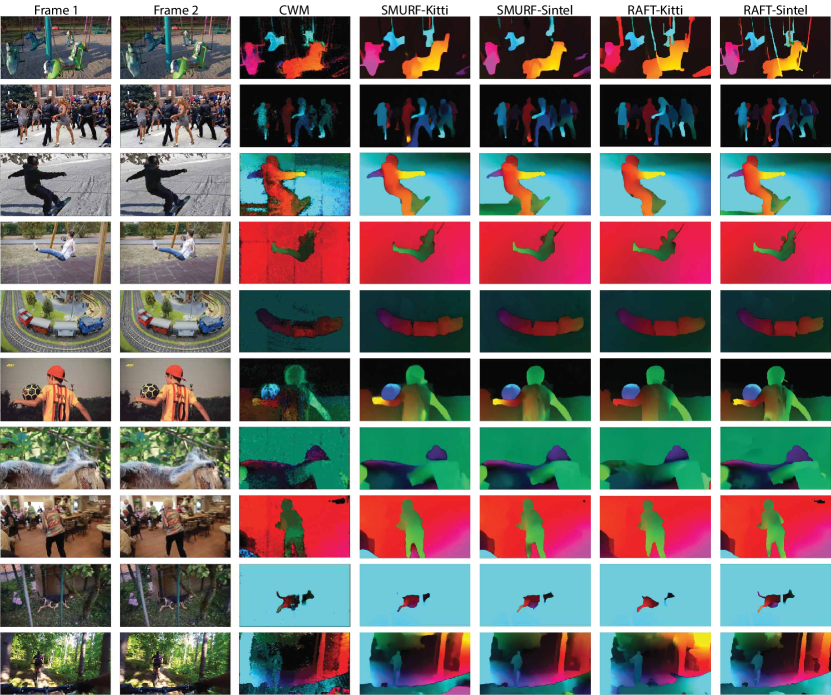
Figure 10: Additional Optical Flows extracted on the DAVIS dataset. To demonstrate the ability of CWM to extract zero-shot unsupervised optical flows, we compare it against two state-of-the-art methods from literature: RAFT and SMURF. RAFT and SMURF are run for 24 iterations each. CWM flows are extracted using Algorithm 5.

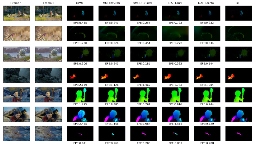
Figure 11: Additional Optical Flows extracted on the Spring dataset. To demonstrate the ability of CWM to extract zero-shot unsupervised optical flows, we compare it against two state of the art methods from literature: RAFT and SMURF. RAFT and SMURF are run for 24 iterations each. CWM flows are extracted using Algorithm 5.

Additional qualitative results on DAVIS and SPRING

We extend the analysis of optical flow extractions by presenting additional qualitative results on two distinct datasets: DAVIS 2016 [65] and a recent synthetic dataset SPRING [50]. The results are shown in Figure 10 and 11 respectively. This evaluation aims to provide a more holistic understanding of the CWM capability in flow estimation, in comparison to task-specific flow estimation methods such as RAFT [78] and SMURF [75] . RAFT is a supervised flow estimation method, whereas SMURF is a self-supervised method. Unlike RAFT and SMURF, CWM is a task-agnostic framework and does not have objectives specific to flow estimation. This comparison emphasizes the differences among various self-supervised learning approaches and underscores the advancements offered by CWM.

We show results from both RAFT and SMURF, each trained on two different datasets: synthetic SINTEL dataset [65] and real-world KITTI dataset [31]. This demonstrates the differences in flow estimation accuracy resulting from different training dataset choice, especially considering that CWM is pre-trained on the real-world Kinetics-400 dataset, akin to the nature of the KITTI dataset. The qualitative results shown in Figures 10 and 11 indicate that CWM consistently exhibits performance comparable to RAFT and SMURF – on both real (DAVIS dataset) and synthetic environments (SPRING dataset).

In Figure 11 we also report the average end-point-error (EPE) [51] on the SPRING dataset alongside qualitative flow visualizations. It is interesting to note that on the SPRING dataset CWM often has lower error compared to the RAFT model supervised on the KITTI dataset.

Additional quantitative results on SPRING

In the main text, we show comparisons between CWM’s zero-shot optical flow and baseline optical flow models supervised or self-supervised on synthetic datasets. Here we include comparisons to models supervised on real-world datasets such as KITTI, which is more aligned with the kind of data that CWM is trained on. In Table 5 we report the results for RAFT [78] and SMURF [75] trained on KITTI dataset. We find that models trained on the synthetic Sintel dataset outperform CWM on the SPRING benchmark, which is expected since SPRING is also a synthetic dataset created in Blender with similar video sequences as Sintel. On the other hand, CWM performs comparably to models trained on real-world KITTI dataset, albeit being outperformed by a small margin. Notably, despite being trained with a different objective (i.e., next frame prediction), CWM gets comparable results to RAFT-KITTI and SMURF-KITTI. This is still a significant result since unlike RAFT and SMURF, which are specifically designed for optical flow estimation, CWM is a general vision foundational model trained with a generic pre-training objective.

3.3 Segmentation

Single Spelke object extraction

To extract the Spelke object at a pixel location $(i,j)$ of a static image, we first create an action that simulates counterfactual motion by taking the patch at location $(i,j)$ and creating a new frame that is largely blank, but in which the content of the patch has been copied (e.g. translated) to a new location $(i\!+\!\epsilon_{1},j\!+\!\epsilon_{2})$, where $\epsilon_{1},\epsilon_{2}$ are location offsets randomly sampled within a radius $r\!>\!0$. We set $r$ to a fixed fraction (0.2) of the input image size. In addition, we can optionally create the appearance of stopping the counterfactual motion at a location $(i^{\prime},j^{\prime})$ by directly copying the patch at that location to the same location in the action without offset (or equivalently $r\!=\!0$). Adding the stop-motion patch allows the counterfactual query to isolate a single object, especially in a cluttered scene with multiple objects adjacent to and stacked on top of one another. In practice, we find that different random choices of motion offset and stop-motion patches could potentially yield different counterfactual motion results. We sample 4 different actions per pixel location, compute flows for the counterfactual motion, average the flow manitudes of the different samples, and then threshold the mean flow magnitude map at 0.5 to obtain the binary segmentation map at pixel location $(i,j)$.

We also find that the above procedure can be repeated iteratively to further refine the segments. Once a tentative segmentation map is obtained, we can sample more patches within the segment and add them to the action to simulate better counterfactual motion. At each iteration, we sample one patch within the segment and add it to the set of patches that simulates counterfactual motion. We additionally sample one patch outside the segment and add it to the set of stop-motion patches that simulates stopping the counterfactual motion. We set the number of iterations to 3 by default.

While the predictor $\Psi$ is trained with input resolution $224\!\times\!224$, Spelke object can be extracted at a different resolution by simply interpolating the position encoding correspondingly. We extract zero-shot segmentations on COCO training images at resolution $480\!\times\!480$ using the ViT-B/8 CWM model.

Multiple Spelke object extraction

To automatically discover multiple Spelke objects in a single image, we choose actions at pixel locations based on a sampling probability distribution $p$, which has high probability at pixel locations belonging to Spelke objects and low otherwise. Once a segment is discovered, we mask out the probability distribution values using the segments and repeat the process to discover the next object.

We find two choices of sampling distribution work well. One is a movability distribution computed by sampling a few random actions and averaging the motion responses across multiple predictions. The second choice is the prominence map computed by applying normalized cut to the patch-wise feature similarity matrix as proposed by CutLER [87]. In practice, the second approach yields slightly better qualitative segmentation results. Therefore, we choose the second approach as the default for computing the sampling probability distribution. Figure LABEL:fig:zero_shot_1 and LABEL:fig:zero_shot_2 show more qualitative segmentation results of Spelke objects extracted by CWM on COCO training images, and compare them to those of other baseline methods FreeSOLO [86] and CutLER [87]. In each image, we set the maximum number of Spelke objects to be extracted as 3.

method	pre-train data	arch	params	OCP by scenario $\uparrow$							Avg. OCP $\uparrow$
				collide	drop	support	link	roll	contain	dominoes
video prediction models
MCVD [82]	K400+Ego4D	UNet	251 M	73.3	65.0	70.7	59.2	51.0	66.7	57.9	63.4
R3M [56]	K400+Ego4D	Res50	38 M	79.0	61.8	70.1	66.9	66.2	62.1	67.3	67.6
FitVid [4]	K400+Ego4D	VAE	303 M	65.0	68.2	71.5	59.9	54.1	60.8	70.7	64.3
TECO [91]	K600	vq-gan	160 M	75.9	70.6	74.4	65.2	59.1	72.4	67.5	69.3
self-supervised image representation models
DINO [12]	IN-1K	ViT-B	86M	79.0	72.6	81.0	72.0	61.8	69.3	69.2	72.1
DINOv2 [60]	LVD-142M	ViT-B	86 M	78.1	70.7	80.3	70.7	64.3	70.6	70.4	72.2
DINOv2 [60]	LVD-142M	ViT-L	304 M	81.0	68.8	82.3	68.8	61.1	69.9	73.6	72.2
DINOv2 [60]	LVD-142M	ViT-g	1.1 B	80.0	74.5	81.0	66.2	61.8	74.5	71.1	72.7
MAE [39]	IN-1K	ViT-B	86 M	80.0	72.6	78.9	70.1	64.3	68.0	74.2	72.6
MAE [39]	IN-1K	ViT-L	304 M	80.0	73.2	81.0	69.4	58.0	69.3	70.4	71.6
MAE [39]	IN-1K	ViT-H	632 M	83.8	72.0	84.4	70.1	61.8	69.3	71.7	73.3
MAE [39]	IN-4.5M	ViT-B	86 M	81.9	70.7	83.0	68.8	59.9	67.3	73.0	72.1
MAE [39]	IN-4.5M	ViT-L	304 M	83.8	70.7	81.0	68.2	59.9	70.6	74.2	72.6
self-supervised video representation models
VMAE [79]	K400	ViT-B	86 M	74.3	74.5	83.0	65.6	61.8	71.2	74.2	72.1
VMAE [79]	K400	ViT-L	304 M	79.0	73.9	82.3	66.9	65.0	72.5	75.5	73.6
VMAE [79]	K400	ViT-H	632 M	81.0	73.2	81.6	70.7	63.1	70.6	74.2	73.5
VMAEv2 [84]	U-Hybrid	ViT-g	1.1B	77.1	75.2	83.0	65.0	62.4	70.6	72.3	72.2
vision-language models
GPT4-V [59]	-	-	-	52.7	46.5	58.5	54.8	56.2	56.1	46.5	52.9
CWM-feat	K400	ViT-B	86 M	81.0	73.2	83.7	65.0	61.8	73.9	76.7	73.6
CWM-feat	K400	ViT-L	304 M	78.1	76.4	83.0	68.8	63.7	73.9	78.0	74.6
CWM	K400	ViT-B	86 M	82.9	75.2	83.7	70.7	63.7	77.8	77.4	75.9
CWM	K400	ViT-L	304 M	83.8	74.5	84.4	71.3	65.0	75.8	78.0	76.1

Table 6: Physion v1.5 scenario-wise OCP results. We compare CWM to four classes of baseline methods across different architectures on the OCP task. In the main text, we presented the scores averaged across all seven scenarios. Here we provide a detailed breakdown of performance for each specific scenario.

method	pre-train data	arch	params	OCD by scenario $\uparrow$							Avg. OCD $\uparrow$
				collide	drop	support	link	roll	contain	dominoes
video prediction models
MCVD [82]	K400+Ego4D	UNet	251 M	82.9	74.5	95.9	75.8	68.8	77.8	89.9	80.8
R3M [56]	K400+Ego4D	Res50	38 M	83.8	72.0	90.5	72.0	72.0	70.6	86.2	78.1
FitVid [4]	K400+Ego4D	VAE	303 M	58.9	56.7	63.1	63.2	60.2	55.5	58.8	59.5
TECO [91]	K600	vq-gan	160 M	87.0	77.5	87.5	70.7	72.6	76.3	95.0	80.9
self-supervised image representation models
DINO [12]	IN-1K	ViT-B	86M	87.6	79.6	95.2	81.5	76.4	80.4	96.9	85.4
DINOv2 [60]	LVD-142M	ViT-B	86 M	89.5	84.7	96.6	86.6	76.4	79.1	96.9	87.1
DINOv2 [60]	LVD-142M	ViT-L	304 M	91.4	79.0	96.6	84.1	73.9	77.8	95.6	85.5
DINOv2 [60]	LVD-142M	ViT-g	1.1 B	91.4	80.3	95.2	83.4	70.1	77.1	94.3	84.6
MAE [39]	IN-1K	ViT-B	86 M	86.7	76.4	92.5	77.7	71.3	72.5	93.7	81.6
MAE [39]	IN-1K	ViT-L	304 M	86.7	75.8	93.9	80.3	70.7	73.2	95.6	82.3
MAE [39]	IN-1K	ViT-H	632 M	84.8	75.2	92.5	76.4	67.5	73.2	96.2	80.8
MAE [39]	IN-4.5M	ViT-B	86 M	86.7	75.8	91.2	76.4	70.7	74.5	96.9	81.7
MAE [39]	IN-4.5M	ViT-L	304 M	89.5	76.4	93.2	77.1	69.4	72.5	95.0	81.9
self-supervised video representation models
VMAE [79]	K400	ViT-B	86 M	91.4	78.3	94.6	80.3	76.4	83.0	95.6	85.7
VMAE [79]	K400	ViT-L	304 M	95.2	78.3	95.2	82.8	75.2	80.4	95.6	86.1
VMAE [79]	K400	ViT-H	632 M	95.2	79.6	95.2	84.7	79.0	81.7	96.9	87.5
VMAEv2 [84]	U-Hybrid	ViT-g	1.1B	91.4	78.3	91.8	84.7	73.9	81.7	93.1	85.0
vision-language models
GPT4-V [59]	-	-	-	52.9	53.0	54.2	60.7	56.2	56.1	49.7	54.7
CWM-feat	K400	ViT-B	86 M	96.2	84.7	95.9	82.8	82.8	84.3	96.9	89.1
CWM-feat	K400	ViT-L	304 M	94.3	83.4	96.6	82.8	83.4	83.0	96.9	88.6
CWM	K400	ViT-B	86 M	96.2	82.2	95.9	85.4	81.5	86.3	96.2	89.1
CWM	K400	ViT-L	304 M	96.2	83.4	96.6	84.1	81.5	83.0	96.2	88.7

Table 7: Physion v1.5 scenario-wise OCD results. We compare CWM to four classes of baseline methods across different architectures on the OCD task. In the main text, we presented the scores averaged across all seven scenarios. Here we provide a detailed breakdown of performance for each specific scenario.

Distillation

Since counterfactual queries for object segmentation can be slow and missing some objects in the image, we follow previous works FreeSOLO [86] and CutLER [87] to distill segmentations extracted from a large task-agnostic pre-trained model into a smaller instance segmenter for faster and more robust segmentation. The extracted segmentations are used as pseudo annotations to train a downstream instance segmenter in a self-supervised manner.

We follow the same procedure in CutLER for training a downstream segmenter. We use Cascade Mask R-CNN as the default segmenter, but CWM is agnostic to the choice of segmenters. The model is trained on COCO train2017 with initial masks and bounding boxes for 160K iterations with a batch size of 32. For a fair comparison to CutLER, we train the detectors with a ResNet-50 backbone, and initialize the model with the weights of a self-supervised pre-trained DINO model. We use SGD with an initial learning rate of 0.005, which is decreased by 5 after 80K iterations. A weight decay of $5\!\times\!10^{-5}$ and a momentum of 0.9 is applied. Since the standard detection loss penalizes predicted regions that do not overlap with the ‘ground-truth’ masks, and the ‘ground-truth’ masks given by CWM may miss instances, the standard loss does not enable the detector to discover new instances not labeled in the ‘ground-truth’. Therefore, we follow CutLER to ignore the loss of predicted regions that have a small overlap with the ‘ground-truth’. We refer the readers to the CutLER paper for more implementation details. Figure LABEL:fig:maskrcnn_1 and LABEL:fig:maskrcnn_2 show the output segmentations of Cascaded Mask R-CNN on COCO validation images after distillation, as compared to prior methods.

4 Dynamics understanding experiments

4.1 Physion benchmark

Dataset details

As discussed in the main text, we use the Physion v1.5 benchmark to evaluate CWM and baseline models on physical dynamics understanding. Physion v1.5 has several key improvements over Physion v1, which are illustrated in Figure LABEL:fig:physion_improvements. More specifically, Physion v1.5 introduces another indoor environment, called the “craft room.”, in addition to the two environments featured in Physion v1 (see Figure LABEL:fig:Rooms). Furthermore, v1.5 enhances the diversity of lighting conditions by employing a collection of 8 unique HDRI skyboxes, specifically designed to simulate various environmental lighting scenarios. This enhancement allows for dynamic time-of-day simulations in the room by adjusting the orientation of the skyboxes and directional lighting (see Figure LABEL:fig:Lighting). Physion v1.5 also has improved rendering quality and photorealism in comparison to v1 (see Figure LABEL:fig:Brightness and  LABEL:fig:Shadows). The physics simulations and rendering are done using the ThreeDWorld simulation platform [30].

Physion v1.5 comprises seven distinct physical scenarios, including collide, drop, dominoes, contain, roll, support, and link. This version comprehensively demonstrates various aspects and challenges of rigid body physics (see Figure LABEL:fig:physion_ocp_results_1 for examples of each scenario). We train and test the linear classifier model (as outlined in Section 4.2 of the main text) on all seven scenarios.

Per-scenario OCP and OCD results.

In the main text, we presented the OCP and OCD scores averaged across all seven scenarios. Now, we provide a detailed breakdown of performance for each specific scenario, as shown in Table 6 and Table 7. We find that CWM achieves superior results on nearly all the scenarios.

Qualitative comparisons on OCP and OCD task.

We supplement our quantitative results on the Physion v1.5 tasks with qualitative visualizations in Figures LABEL:fig:physion_ocp_results_1, LABEL:fig:physion_ocp_results_2, LABEL:fig:physion_ocd_results_1 and LABEL:fig:physion_ocd_results_2. We show several example inputs for each scenario, along with the classification results of a linear probe on top of the CWM model, compared with those of leading baselines in each model category outlined in Table 2 in the main text.

Integrating vision structures for OCP and OCD tasks.

In the main text, we demonstrate how zero-shot vision structures extracted from CWM improve OCP and OCD performance on Physion v1.5. This section describes the details of how these structures are integrated prior to linear probing on downstream tasks. Keypoint information is integrated by incorporating patch features at the keypoint locations. Optical flow information is integrated by providing $8\times 8$ patches of optical flow value at the keypoint locations. Finally, segment information is integrated by using the segments to pool the feature map and incorporate the aggregated features for linear probing.

The integration process for segments is detailed as follows: Let $F\!\in\!\mathbb{R}^{H\times W\times D}$ be the feature map of an input frame from the last layer of the ViT encoder, where $H$, $W$, and $D$ represent height, width, and channel dimension. Suppose we have binary segmentation masks $S$ with dimension $N\times H\times W$, where $N$ denotes the number of masks. We compute the set of aggregated feature vectors for each of the segments,

$$F_{agg}=\left\{\frac{\sum_{i,j}S^{n}_{ij}F_{ij}}{\sum_{i,j}S^{n}_{ij}}\,\mid\,1\leq n\leq N\right\}$$ (6)

where $S^{n}$ is the $n$-th segmentation mask and $F_{ij}$ is the feature vector at location $(i,j)$. These aggregated feature vectors, along with the keypoint patch features and flow patches, are concatenated with the original feature map $F$ before being fed into the linear classifier.

4.2 GPT4-Vision prompting

GPT-4V prompting methodology and results.

In Figures LABEL:fig:gpt_results_1, LABEL:fig:gpt_results_2, LABEL:fig:gpt_results_3 and  LABEL:fig:gpt_results_4 we report a few results from testing GPT-4V on the OCP and OCD tasks in Physion v1.5. In each figure, the prompt image is shown on the left and the prompt text along with the GT label and response is shown on the right. To construct the image prompt, we tile four successive video frames (sampled at a frame gap of 150ms) into a $2\!\times\!2$ image with four panels. Each panel contains an RGB frame titled with its timestamp. Following the methodology used for evaluating vision-only models, the objects of interest for the contact-related queries are rendered with red and yellow textures to provide visual cues for the model. For OCP, the text prompt used was “These are 4 images taken sequentially from a video. If the video were to continue, would the red object touch the yellow surface? Explain your thinking and end with True or False only”. For OCD, the prompt used was “These are 4 images taken sequentially from a video. Does the red object touch the yellow surface at any point in the video? Explain your thinking and end with True or False only”. GPT4-V achieves 52.9% accuracy for OCP and 54.7% accuracy for OCD. For OCP, the model predicted “contact” 78.7% of the time, while for OCD the model predicted “no contact” 81.5% of the time.

Prompting Method	OCP $\uparrow$	OCD $\uparrow$
RGB frames	52.9	54.7
RGB frames + GT segment overlay	58.3	67.5

Table 8: GPT-4V performance on the Physion v1.5 tasks using two different promoting strategies: a) with RGB frames only and b) RGB frames with ground truth segment map overlayed on the objects of interest.

Alternate querying methods.

Additionally, we experiment with an alternative querying method to explore the limit of GPT4-V in dynamics understanding. In addition to rendering the objects of interest in red and yellow texture, we apply a bright red and yellow ground-truth segmentation overlay on them to focus the model’s attention on these objects (see Figure LABEL:fig:gpt_results_1 for visualizations). As shown in Table 8, we find that this querying strategy improves the OCP from 52.9% to 58.3% and the OCD from 54.7% to 67.5%. In the main text, we have also demonstrated a parallel phenomenon with CWM, where integrating segment information led to enhanced performance in related tasks (Table 3e in main text). These observations highlight the importance of vision structures such as segmentation in downstream tasks associated with physical dynamics understanding.

Implementation details.

We employ four GPT-4V accounts and retrieve the results using Selenium [26], a browser automation tool. Our methodology adheres to the code framework available at.

References

- Agrawal et al. [2016] Pulkit Agrawal, Ashvin V Nair, Pieter Abbeel, Jitendra Malik, and Sergey Levine. Learning to poke by poking: Experiential learning of intuitive physics. Advances in neural information processing systems, 29, 2016.
- Ajay et al. [2019] Anurag Ajay, Maria Bauza, Jiajun Wu, Nima Fazeli, Joshua B Tenenbaum, Alberto Rodriguez, and Leslie P Kaelbling. Combining physical simulators and object-based networks for control. In 2019 International Conference on Robotics and Automation (ICRA), pages 3217–3223. IEEE, 2019.
- Awadalla et al. [2023] Anas Awadalla, Irena Gao, Josh Gardner, Jack Hessel, Yusuf Hanafy, Wanrong Zhu, Kalyani Marathe, Yonatan Bitton, Samir Gadre, Shiori Sagawa, Jenia Jitsev, Simon Kornblith, Pang Wei Koh, Gabriel Ilharco, Mitchell Wortsman, and Ludwig Schmidt. Openflamingo: An open-source framework for training large autoregressive vision-language models. arXiv preprint arXiv:2308.01390, 2023.
- Babaeizadeh et al. [2021] Mohammad Babaeizadeh, Mohammad Taghi Saffar, Suraj Nair, Sergey Levine, Chelsea Finn, and Dumitru Erhan. Fitvid: Overfitting in pixel-level video prediction. arXiv preprint arXiv:2106.13195, 2021.
- Bakhtin et al. [2019] Anton Bakhtin, Laurens van der Maaten, Justin Johnson, Laura Gustafson, and Ross Girshick. Phyre: A new benchmark for physical reasoning. Advances in Neural Information Processing Systems, 32, 2019.
- Bao et al. [2021] Hangbo Bao, Li Dong, Songhao Piao, and Furu Wei. Beit: Bert pre-training of image transformers. arXiv preprint arXiv:2106.08254, 2021.
- Bates et al. [2019] Christopher J Bates, Ilker Yildirim, Joshua B Tenenbaum, and Peter Battaglia. Modeling human intuitions about liquid flow with particle-based simulation. PLoS computational biology, 15(7):e1007210, 2019.
- Battaglia et al. [2016] Peter Battaglia, Razvan Pascanu, Matthew Lai, Danilo Jimenez Rezende, et al. Interaction networks for learning about objects, relations and physics. Advances in neural information processing systems, 29, 2016.
- Bear et al. [2021] Daniel M Bear, Elias Wang, Damian Mrowca, Felix J Binder, Hsiao-Yu Fish Tung, RT Pramod, Cameron Holdaway, Sirui Tao, Kevin Smith, Fan-Yun Sun, et al. Physion: Evaluating physical prediction from vision in humans and machines. arXiv preprint arXiv:2106.08261, 2021.
- Bear et al. [2023] Daniel M Bear, Kevin Feigelis, Honglin Chen, Wanhee Lee, Rahul Venkatesh, Klemen Kotar, Alex Durango, and Daniel LK Yamins. Unifying (machine) vision via counterfactual world modeling. arXiv preprint arXiv:2306.01828, 2023.
- Cai and Vasconcelos [2018] Zhaowei Cai and Nuno Vasconcelos. Cascade r-cnn: Delving into high quality object detection. In Proceedings of the IEEE conference on computer vision and pattern recognition, pages 6154–6162, 2018.
- Caron et al. [2021] Mathilde Caron, Hugo Touvron, Ishan Misra, Hervé Jégou, Julien Mairal, Piotr Bojanowski, and Armand Joulin. Emerging properties in self-supervised vision transformers. In Proceedings of the International Conference on Computer Vision (ICCV), 2021.
- Chen et al. [2022a] Honglin Chen, Wanhee Lee, Hong-Xing Yu, Rahul Mysore Venkatesh, Joshua B Tenenbaum, Daniel Bear, Jiajun Wu, and Daniel LK Yamins. Unsupervised 3d scene representation learning via movable object inference. 2022a.
- Chen et al. [2022b] Honglin Chen, Rahul Venkatesh, Yoni Friedman, Jiajun Wu, Joshua B Tenenbaum, Daniel LK Yamins, and Daniel M Bear. Unsupervised segmentation in real-world images via spelke object inference. In European Conference on Computer Vision, pages 719–735. Springer, 2022b.
- Chen et al. [2023a] Jun Chen, Deyao Zhu, Xiaoqian Shen, Xiang Li, Zechu Liu, Pengchuan Zhang, Raghuraman Krishnamoorthi, Vikas Chandra, Yunyang Xiong, and Mohamed Elhoseiny. Minigpt-v2: large language model as a unified interface for vision-language multi-task learning. arXiv preprint arXiv:2310.09478, 2023a.
- Chen et al. [2020a] Mark Chen, Alec Radford, Rewon Child, Jeffrey Wu, Heewoo Jun, David Luan, and Ilya Sutskever. Generative pretraining from pixels. In International conference on machine learning, pages 1691–1703. PMLR, 2020a.
- Chen et al. [2020b] Ting Chen, Simon Kornblith, Mohammad Norouzi, and Geoffrey Hinton. A simple framework for contrastive learning of visual representations. In International conference on machine learning, pages 1597–1607. PMLR, 2020b.
- Chen et al. [2023b] Xinyuan Chen, Yaohui Wang, Lingjun Zhang, Shaobin Zhuang, Xin Ma, Jiashuo Yu, Yali Wang, Dahua Lin, Yu Qiao, and Ziwei Liu. Seine: Short-to-long video diffusion model for generative transition and prediction. arXiv preprint arXiv:2310.20700, 2023b.
- Chowdhery et al. [2022] Aakanksha Chowdhery, Sharan Narang, Jacob Devlin, Maarten Bosma, Gaurav Mishra, Adam Roberts, Paul Barham, Hyung Won Chung, Charles Sutton, Sebastian Gehrmann, et al. Palm: Scaling language modeling with pathways. arXiv preprint arXiv:2204.02311, 2022.
- Dave et al. [2022] Ishan Dave, Rohit Gupta, Mamshad Nayeem Rizve, and Mubarak Shah. Tclr: Temporal contrastive learning for video representation. Computer Vision and Image Understanding, 219:103406, 2022.
- Doersch et al. [2015] Carl Doersch, Abhinav Gupta, and Alexei A Efros. Unsupervised visual representation learning by context prediction. In Proceedings of the IEEE international conference on computer vision, pages 1422–1430, 2015.
- Dosovitskiy et al. [2020] Alexey Dosovitskiy, Lucas Beyer, Alexander Kolesnikov, Dirk Weissenborn, Xiaohua Zhai, Thomas Unterthiner, Mostafa Dehghani, Matthias Minderer, Georg Heigold, Sylvain Gelly, et al. An image is worth 16x16 words: Transformers for image recognition at scale. arXiv preprint arXiv:2010.11929, 2020.
- Du et al. [2020] Yilun Du, Kevin Smith, Tomer Ulman, Joshua Tenenbaum, and Jiajun Wu. Unsupervised discovery of 3d physical objects from video. arXiv preprint arXiv:2007.12348, 2020.
- Du et al. [2022] Zhengxiao Du, Yujie Qian, Xiao Liu, Ming Ding, Jiezhong Qiu, Zhilin Yang, and Jie Tang. Glm: General language model pretraining with autoregressive blank infilling. In Proceedings of the 60th Annual Meeting of the Association for Computational Linguistics (Volume 1: Long Papers), pages 320–335, 2022.
- Ebert et al. [2021] Frederik Ebert, Yanlai Yang, Karl Schmeckpeper, Bernadette Bucher, Georgios Georgakis, Kostas Daniilidis, Chelsea Finn, and Sergey Levine. Bridge data: Boosting generalization of robotic skills with cross-domain datasets. arXiv preprint arXiv:2109.13396, 2021.
- [26] elenium Contributors. Selenium: Browser automation framework.
- Feichtenhofer et al. [2022] Christoph Feichtenhofer, Yanghao Li, Kaiming He, et al. Masked autoencoders as spatiotemporal learners. Advances in neural information processing systems, 35:35946–35958, 2022.
- Finn and Levine [2017] Chelsea Finn and Sergey Levine. Deep visual foresight for planning robot motion. In 2017 IEEE International Conference on Robotics and Automation (ICRA), pages 2786–2793. IEEE, 2017.
- Fragkiadaki et al. [2015] Katerina Fragkiadaki, Pulkit Agrawal, Sergey Levine, and Jitendra Malik. Learning visual predictive models of physics for playing billiards. arXiv preprint arXiv:1511.07404, 2015.
- Gan et al. [2020] Chuang Gan, Jeremy Schwartz, Seth Alter, Damian Mrowca, Martin Schrimpf, James Traer, Julian De Freitas, Jonas Kubilius, Abhishek Bhandwaldar, Nick Haber, et al. Threedworld: A platform for interactive multi-modal physical simulation. arXiv preprint arXiv:2007.04954, 2020.
- Geiger et al. [2013] Andreas Geiger, Philip Lenz, Christoph Stiller, and Raquel Urtasun. Vision meets robotics: The kitti dataset. The International Journal of Robotics Research, 32(11):1231–1237, 2013.
- Gidaris et al. [2018] Spyros Gidaris, Praveer Singh, and Nikos Komodakis. Unsupervised representation learning by predicting image rotations. arXiv preprint arXiv:1803.07728, 2018.
- Goyal et al. [2017] Priya Goyal, Piotr Dollár, Ross Girshick, Pieter Noordhuis, Lukasz Wesolowski, Aapo Kyrola, Andrew Tulloch, Yangqing Jia, and Kaiming He. Accurate, large minibatch sgd: Training imagenet in 1 hour. arXiv preprint arXiv:1706.02677, 2017.
- Groth et al. [2018] Oliver Groth, Fabian B Fuchs, Ingmar Posner, and Andrea Vedaldi. Shapestacks: Learning vision-based physical intuition for generalised object stacking. In Proceedings of the european conference on computer vision (eccv), pages 702–717, 2018.
- Gupta et al. [2022] Agrim Gupta, Stephen Tian, Yunzhi Zhang, Jiajun Wu, Roberto Martín-Martín, and Li Fei-Fei. Maskvit: Masked visual pre-training for video prediction. arXiv preprint arXiv:2206.11894, 2022.
- Hafner et al. [2019a] Danijar Hafner, Timothy Lillicrap, Jimmy Ba, and Mohammad Norouzi. Dream to control: Learning behaviors by latent imagination. arXiv preprint arXiv:1912.01603, 2019a.
- Hafner et al. [2019b] Danijar Hafner, Timothy Lillicrap, Ian Fischer, Ruben Villegas, David Ha, Honglak Lee, and James Davidson. Learning latent dynamics for planning from pixels. In International conference on machine learning, pages 2555–2565. PMLR, 2019b.
- He et al. [2020] Kaiming He, Haoqi Fan, Yuxin Wu, Saining Xie, and Ross Girshick. Momentum contrast for unsupervised visual representation learning. In Proceedings of the IEEE/CVF conference on computer vision and pattern recognition, pages 9729–9738, 2020.
- He et al. [2022] Kaiming He, Xinlei Chen, Saining Xie, Yanghao Li, Piotr Dollár, and Ross Girshick. Masked autoencoders are scalable vision learners. In Proceedings of the IEEE/CVF conference on computer vision and pattern recognition, pages 16000–16009, 2022.
- Hoffmann et al. [2022] Jordan Hoffmann, Sebastian Borgeaud, Arthur Mensch, Elena Buchatskaya, Trevor Cai, Eliza Rutherford, Diego de Las Casas, Lisa Anne Hendricks, Johannes Welbl, Aidan Clark, et al. Training compute-optimal large language models. arXiv preprint arXiv:2203.15556, 2022.
- Höppe et al. [2022] Tobias Höppe, Arash Mehrjou, Stefan Bauer, Didrik Nielsen, and Andrea Dittadi. Diffusion models for video prediction and infilling. arXiv preprint arXiv:2206.07696, 2022.
- Karazija et al. [2022] Laurynas Karazija, Subhabrata Choudhury, Iro Laina, Christian Rupprecht, and Andrea Vedaldi. Unsupervised multi-object segmentation by predicting probable motion patterns. Advances in Neural Information Processing Systems, 35:2128–2141, 2022.
- Kay et al. [2017] Will Kay, Joao Carreira, Karen Simonyan, Brian Zhang, Chloe Hillier, Sudheendra Vijayanarasimhan, Fabio Viola, Tim Green, Trevor Back, Paul Natsev, et al. The kinetics human action video dataset. arXiv preprint arXiv:1705.06950, 2017.
- Li et al. [2018] Yunzhu Li, Jiajun Wu, Russ Tedrake, Joshua B Tenenbaum, and Antonio Torralba. Learning particle dynamics for manipulating rigid bodies, deformable objects, and fluids. arXiv preprint arXiv:1810.01566, 2018.
- Lin et al. [2014] Tsung-Yi Lin, Michael Maire, Serge Belongie, James Hays, Pietro Perona, Deva Ramanan, Piotr Dollár, and C Lawrence Zitnick. Microsoft coco: Common objects in context. In Computer Vision–ECCV 2014: 13th European Conference, Zurich, Switzerland, September 6-12, 2014, Proceedings, Part V 13, pages 740–755. Springer, 2014.
- Locatello et al. [2020] Francesco Locatello, Dirk Weissenborn, Thomas Unterthiner, Aravindh Mahendran, Georg Heigold, Jakob Uszkoreit, Alexey Dosovitskiy, and Thomas Kipf. Object-centric learning with slot attention. Advances in Neural Information Processing Systems, 33:11525–11538, 2020.
- Loshchilov and Hutter [2016] Ilya Loshchilov and Frank Hutter. Sgdr: Stochastic gradient descent with warm restarts. arXiv preprint arXiv:1608.03983, 2016.
- Loshchilov and Hutter [2017] Ilya Loshchilov and Frank Hutter. Decoupled weight decay regularization. arXiv preprint arXiv:1711.05101, 2017.
- Lu et al. [2023] Haoyu Lu, Guoxing Yang, Nanyi Fei, Yuqi Huo, Zhiwu Lu, Ping Luo, and Mingyu Ding. Vdt: An empirical study on video diffusion with transformers. arXiv preprint arXiv:2305.13311, 2023.
- Mehl et al. [2023a] Lukas Mehl, Jenny Schmalfuss, Azin Jahedi, Yaroslava Nalivayko, and Andrés Bruhn. Spring: A high-resolution high-detail dataset and benchmark for scene flow, optical flow and stereo. In Proc. IEEE/CVF Conference on Computer Vision and Pattern Recognition (CVPR), 2023a.
- Mehl et al. [2023b] Lukas Mehl, Jenny Schmalfuss, Azin Jahedi, Yaroslava Nalivayko, and Andrés Bruhn. Spring: A high-resolution high-detail dataset and benchmark for scene flow, optical flow and stereo. arXiv preprint arXiv:2303.01943, 2023b.
- Mian et al. [2008] Ajmal S Mian, Mohammed Bennamoun, and Robyn Owens. Keypoint detection and local feature matching for textured 3d face recognition. International Journal of Computer Vision, 79:1–12, 2008.
- Minderer et al. [2019] Matthias Minderer, Chen Sun, Ruben Villegas, Forrester Cole, Kevin P Murphy, and Honglak Lee. Unsupervised learning of object structure and dynamics from videos. Advances in Neural Information Processing Systems, 32, 2019.
- Mottaghi et al. [2016] Roozbeh Mottaghi, Hessam Bagherinezhad, Mohammad Rastegari, and Ali Farhadi. Newtonian scene understanding: Unfolding the dynamics of objects in static images. In Proceedings of the IEEE Conference on Computer Vision and Pattern Recognition, pages 3521–3529, 2016.
- Mrowca et al. [2018] Damian Mrowca, Chengxu Zhuang, Elias Wang, Nick Haber, Li F Fei-Fei, Josh Tenenbaum, and Daniel L Yamins. Flexible neural representation for physics prediction. Advances in neural information processing systems, 31, 2018.
- Nair et al. [2022] Suraj Nair, Aravind Rajeswaran, Vikash Kumar, Chelsea Finn, and Abhinav Gupta. R3m: A universal visual representation for robot manipulation. arXiv preprint arXiv:2203.12601, 2022.
- Noroozi and Favaro [2016] Mehdi Noroozi and Paolo Favaro. Unsupervised learning of visual representations by solving jigsaw puzzles. In European conference on computer vision, pages 69–84. Springer, 2016.
- Oord et al. [2018] Aaron van den Oord, Yazhe Li, and Oriol Vinyals. Representation learning with contrastive predictive coding. arXiv preprint arXiv:1807.03748, 2018.
- OpenAI [2023] OpenAI. Gpt-4 for vision (chatgpt with image input), 2023. Accessed: October 27, 2023.
- Oquab et al. [2023] Maxime Oquab, Timothée Darcet, Theo Moutakanni, Huy V. Vo, Marc Szafraniec, Vasil Khalidov, Pierre Fernandez, Daniel Haziza, Francisco Massa, Alaaeldin El-Nouby, Russell Howes, Po-Yao Huang, Hu Xu, Vasu Sharma, Shang-Wen Li, Wojciech Galuba, Mike Rabbat, Mido Assran, Nicolas Ballas, Gabriel Synnaeve, Ishan Misra, Herve Jegou, Julien Mairal, Patrick Labatut, Armand Joulin, and Piotr Bojanowski. Dinov2: Learning robust visual features without supervision, 2023.
- Otte and Nagel [1994] Michael Otte and H H Nagel. Optical flow estimation: advances and comparisons. In Computer Vision—ECCV’94: Third European Conference on Computer Vision Stockholm, Sweden, May 2–6, 1994 Proceedings, Volume I 3, pages 49–60. Springer, 1994.
- Pathak et al. [2017] Deepak Pathak, Ross Girshick, Piotr Dollár, Trevor Darrell, and Bharath Hariharan. Learning features by watching objects move. In Proceedings of the IEEE conference on computer vision and pattern recognition, pages 2701–2710, 2017.
- Perazzi et al. [2016] F. Perazzi, J. Pont-Tuset, B. McWilliams, L. Van Gool, M. Gross, and A. Sorkine-Hornung. A benchmark dataset and evaluation methodology for video object segmentation. In Computer Vision and Pattern Recognition, 2016.
- Piloto et al. [2022] Luis S Piloto, Ari Weinstein, Peter Battaglia, and Matthew Botvinick. Intuitive physics learning in a deep-learning model inspired by developmental psychology. Nature human behaviour, 6(9):1257–1267, 2022.
- Pont-Tuset et al. [2017] J. Pont-Tuset, F. Perazzi, S. Caelles, P. Arbelaez, A. Sorkine-Hornung, and L. Van Gool. The 2017 davis challenge on video object segmentation. arXiv preprint arXiv:1704.00675, 2017.
- Qi et al. [2020] Haozhi Qi, Xiaolong Wang, Deepak Pathak, Yi Ma, and Jitendra Malik. Learning long-term visual dynamics with region proposal interaction networks. arXiv preprint arXiv:2008.02265, 2020.
- Qian et al. [2021] Rui Qian, Tianjian Meng, Boqing Gong, Ming-Hsuan Yang, Huisheng Wang, Serge Belongie, and Yin Cui. Spatiotemporal contrastive video representation learning. In Proceedings of the IEEE/CVF Conference on Computer Vision and Pattern Recognition, pages 6964–6974, 2021.
- Ranjan and Black [2017] Anurag Ranjan and Michael J Black. Optical flow estimation using a spatial pyramid network. In Proceedings of the IEEE conference on computer vision and pattern recognition, pages 4161–4170, 2017.
- Riochet et al. [2021] Ronan Riochet, Mario Ynocente Castro, Mathieu Bernard, Adam Lerer, Rob Fergus, Véronique Izard, and Emmanuel Dupoux. Intphys 2019: A benchmark for visual intuitive physics understanding. IEEE Transactions on Pattern Analysis and Machine Intelligence, 44(9):5016–5025, 2021.
- Sanchez-Gonzalez et al. [2018] Alvaro Sanchez-Gonzalez, Nicolas Heess, Jost Tobias Springenberg, Josh Merel, Martin Riedmiller, Raia Hadsell, and Peter Battaglia. Graph networks as learnable physics engines for inference and control. In International Conference on Machine Learning, pages 4470–4479. PMLR, 2018.
- Shen et al. [2023] Yongliang Shen, Kaitao Song, Xu Tan, Dongsheng Li, Weiming Lu, and Yueting Zhuang. Hugginggpt: Solving ai tasks with chatgpt and its friends in huggingface. arXiv preprint arXiv:2303.17580, 2023.
- Sitzmann et al. [2019] Vincent Sitzmann, Michael Zollhöfer, and Gordon Wetzstein. Scene representation networks: Continuous 3d-structure-aware neural scene representations. Advances in Neural Information Processing Systems, 32, 2019.
- Smith et al. [2019] Kevin Smith, Lingjie Mei, Shunyu Yao, Jiajun Wu, Elizabeth Spelke, Josh Tenenbaum, and Tomer Ullman. Modeling expectation violation in intuitive physics with coarse probabilistic object representations. Advances in neural information processing systems, 32, 2019.
- Spelke [1990] Elizabeth S Spelke. Principles of object perception. Cognitive science, 14(1):29–56, 1990.
- Stone et al. [2021] Austin Stone, Daniel Maurer, Alper Ayvaci, Anelia Angelova, and Rico Jonschkowski. Smurf: Self-teaching multi-frame unsupervised raft with full-image warping. In Proceedings of the IEEE/CVF conference on Computer Vision and Pattern Recognition, pages 3887–3896, 2021.
- Sun et al. [2018] Deqing Sun, Xiaodong Yang, Ming-Yu Liu, and Jan Kautz. Pwc-net: Cnns for optical flow using pyramid, warping, and cost volume. In Proceedings of the IEEE conference on computer vision and pattern recognition, pages 8934–8943, 2018.
- Tacchetti et al. [2018] Andrea Tacchetti, H Francis Song, Pedro AM Mediano, Vinicius Zambaldi, Neil C Rabinowitz, Thore Graepel, Matthew Botvinick, and Peter W Battaglia. Relational forward models for multi-agent learning. arXiv preprint arXiv:1809.11044, 2018.
- Teed and Deng [2020] Zachary Teed and Jia Deng. Raft: Recurrent all-pairs field transforms for optical flow. In Computer Vision–ECCV 2020: 16th European Conference, Glasgow, UK, August 23–28, 2020, Proceedings, Part II 16, pages 402–419. Springer, 2020.
- Tong et al. [2022] Zhan Tong, Yibing Song, Jue Wang, and Limin Wang. Videomae: Masked autoencoders are data-efficient learners for self-supervised video pre-training. Advances in neural information processing systems, 35:10078–10093, 2022.
- Touvron et al. [2023] Hugo Touvron, Thibaut Lavril, Gautier Izacard, Xavier Martinet, Marie-Anne Lachaux, Timothée Lacroix, Baptiste Rozière, Naman Goyal, Eric Hambro, Faisal Azhar, et al. Llama: Open and efficient foundation language models. arXiv preprint arXiv:2302.13971, 2023.
- Tung et al. [2023] Hsiao-Yu Tung, Mingyu Ding, Zhenfang Chen, Daniel Bear, Chuang Gan, Joshua B Tenenbaum, Daniel LK Yamins, Judith E Fan, and Kevin A Smith. Physion++: Evaluating physical scene understanding that requires online inference of different physical properties. arXiv preprint arXiv:2306.15668, 2023.
- Voleti et al. [2022] Vikram Voleti, Alexia Jolicoeur-Martineau, and Chris Pal. Mcvd-masked conditional video diffusion for prediction, generation, and interpolation. Advances in Neural Information Processing Systems, 35:23371–23385, 2022.
- Wang et al. [2018] Limin Wang, Yuanjun Xiong, Zhe Wang, Yu Qiao, Dahua Lin, Xiaoou Tang, and Luc Van Gool. Temporal segment networks for action recognition in videos. IEEE transactions on pattern analysis and machine intelligence, 41(11):2740–2755, 2018.
- Wang et al. [2023a] Limin Wang, Bingkun Huang, Zhiyu Zhao, Zhan Tong, Yinan He, Yi Wang, Yali Wang, and Yu Qiao. Videomae v2: Scaling video masked autoencoders with dual masking. In Proceedings of the IEEE/CVF Conference on Computer Vision and Pattern Recognition, pages 14549–14560, 2023a.
- Wang and Gupta [2015] Xiaolong Wang and Abhinav Gupta. Unsupervised learning of visual representations using videos. In Proceedings of the IEEE international conference on computer vision, pages 2794–2802, 2015.
- Wang et al. [2022] Xinlong Wang, Zhiding Yu, Shalini De Mello, Jan Kautz, Anima Anandkumar, Chunhua Shen, and Jose M Alvarez. Freesolo: Learning to segment objects without annotations. In Proceedings of the IEEE/CVF Conference on Computer Vision and Pattern Recognition, pages 14176–14186, 2022.
- Wang et al. [2023b] Xudong Wang, Rohit Girdhar, Stella X Yu, and Ishan Misra. Cut and learn for unsupervised object detection and instance segmentation. In Proceedings of the IEEE/CVF Conference on Computer Vision and Pattern Recognition, pages 3124–3134, 2023b.
- Wang et al. [2023c] Yangtao Wang, Xi Shen, Yuan Yuan, Yuming Du, Maomao Li, Shell Xu Hu, James L Crowley, and Dominique Vaufreydaz. Tokencut: Segmenting objects in images and videos with self-supervised transformer and normalized cut. IEEE Transactions on Pattern Analysis and Machine Intelligence, 2023c.
- Wu et al. [2018] Zhirong Wu, Yuanjun Xiong, Stella X Yu, and Dahua Lin. Unsupervised feature learning via non-parametric instance discrimination. In Proceedings of the IEEE conference on computer vision and pattern recognition, pages 3733–3742, 2018.
- Wu et al. [2022] Ziyi Wu, Nikita Dvornik, Klaus Greff, Thomas Kipf, and Animesh Garg. Slotformer: Unsupervised visual dynamics simulation with object-centric models. arXiv preprint arXiv:2210.05861, 2022.
- Yan et al. [2023] Wilson Yan, Danijar Hafner, Stephen James, and Pieter Abbeel. Temporally consistent transformers for video generation. 2023.
- Ye et al. [2019] Yufei Ye, Maneesh Singh, Abhinav Gupta, and Shubham Tulsiani. Compositional video prediction. In Proceedings of the IEEE/CVF International Conference on Computer Vision, pages 10353–10362, 2019.
- Yu et al. [2021a] Alex Yu, Vickie Ye, Matthew Tancik, and Angjoo Kanazawa. pixelnerf: Neural radiance fields from one or few images. In Proceedings of the IEEE/CVF Conference on Computer Vision and Pattern Recognition, pages 4578–4587, 2021a.
- Yu et al. [2021b] Hong-Xing Yu, Leonidas J Guibas, and Jiajun Wu. Unsupervised discovery of object radiance fields. arXiv preprint arXiv:2107.07905, 2021b.
- Yu et al. [2023] Lijun Yu, Yong Cheng, Kihyuk Sohn, José Lezama, Han Zhang, Huiwen Chang, Alexander G Hauptmann, Ming-Hsuan Yang, Yuan Hao, Irfan Essa, et al. Magvit: Masked generative video transformer. In Proceedings of the IEEE/CVF Conference on Computer Vision and Pattern Recognition, pages 10459–10469, 2023.
- Zhang et al. [2016] Richard Zhang, Phillip Isola, and Alexei A Efros. Colorful image colorization. In Computer Vision–ECCV 2016: 14th European Conference, Amsterdam, The Netherlands, October 11-14, 2016, Proceedings, Part III 14, pages 649–666. Springer, 2016.
- Zhuang et al. [2020] Chengxu Zhuang, Tianwei She, Alex Andonian, Max Sobol Mark, and Daniel Yamins. Unsupervised learning from video with deep neural embeddings. In Proceedings of the ieee/cvf conference on computer vision and pattern recognition, pages 9563–9572, 2020.
1