SkyScenes: A Synthetic Dataset for Aerial Scene Understanding

Abstract

Real-world aerial scene understanding is limited by a lack of datasets that contain densely annotated images curated under a diverse set of conditions. Due to inherent challenges in obtaining such images in controlled real-world settings, we present SkyScenes, a synthetic dataset of densely annotated aerial images captured from Unmanned Aerial Vehicle (UAV) perspectives. We carefully curate SkyScenes images from Carla to comprehensively capture diversity across layout (urban and rural maps), weather conditions, times of day, pitch angles and altitudes with corresponding semantic, instance and depth annotations. Through our experiments using SkyScenes, we show that (1) Models trained on SkyScenes generalize well to different real-world scenarios, (2) augmenting training on real images with SkyScenes data can improve real-world performance, (3) controlled variations in SkyScenes can offer insights into how models respond to changes in viewpoint conditions, and (4) incorporating additional sensor modalities (depth) can improve aerial scene understanding.

Figure 1: Overview. SkyScenes comprises of $33.6$K aerial images curated from UAV perspectives under different weather and daytime conditions (col $1$), different flying altitudes (col $2$), different viewpoint pitch angles (col $3$), different map layouts (rural and urban, col $5$) with supporting dense pixel level semantic, and depth annotations (col $4$). SkyScenes not only serves as a synthetic source dataset to train real-world generalizable models, but can also augment real data for improved real-world performance.

Dataset

Reproducibility

Diversity

Annotations

Image Capture

Scale

Metadata

Contr. Var.

Town

Daytime

Weather

Semantic

Instance

Depth

Altitude

Perspective

Resolution

Real

1 UAVid [19]

✗

✗

✓

✗

✗

✓

✗

✗

Med

Obl.

$3840\times 2160$

$0.42$K

2 AeroScapes [22]

✗

✗

✗

✗

✗

✓

✗

✗

(Low, Med)

(Obl., Nad.)

$1280\times 720$

$3.27$K

3 ICG Drone [14]

✗

✗

✗

✗

✗

✓

✗

✗

Low

Nad.

$6000\times 4000$

$0.6$K

Synthetic

4 MidAir [9]

✓

partial

✓

✓

✓

✓

✗

✓

Low

(Obl., Nad.)

$1024\times 1024$

$119$K

5 VALID [2]

✗

✗

✓

✓

✓

✓

✓

✓

(Low, Med, High)

Nad.

$1024\times 1024$

$6.7$K

6 Espada [17]

✗

✗

✓

✗

✗

✗

✗

✓

(Med, High)

Nad.

$640\times 480$

$80$K

7 TartanAir [35]

✓

*

✓

✓

✓

✓

✗

✓

Low

(Fwd., Obl.)

$640\times 480$

$\sim 1$M

8 UrbanScene3D [16]

*

*

✓

*

*

✗

✗

✗

Med

Obl.

$6000\times 4000$

$128$K

9 SynthAer [30]

✓

✓

✗

✓

✗

✓

✗

✗

(Low, Med)

Obl.

$1280\times 720$

$\sim 0.77$K

10 SynDrone [25]

✓

✗

✓

✗

✗

✓

✗

✓

(Low, Med, High)

(Obl., Nad.)

$1920\times 1080$

$72$K

11 SkyScenes

✓

✓

✓

✓

✓

✓

✓

✓

(Low, Med, High)

(Fwd., Obl., Nad.)

$2160\times 1440$

$33.6$K

Table 1: SkyScenes compared with other Real and Synthetic Datasets. We compare SkyScenes (row $11$) with other real (rows $1-3$) and synthetic (rows $4-10$) aerial datasets across several axes: (i) Reproducibility – the ability to reproduce the same exact viewpoint under different Controlled Variations (Contr. Var.) from fine-grained scene Metadata, (ii) Diversity – diversity of map layouts (rural, urban), weather and daytime conditions in the provided images, (iii) Annotations – supporting dense annotations for images, (iv) Image Capture – conditions under which images are captured, and (v) Scale – number of images. We see that while existing datasets might be lacking in a subset of criteria, SkyScenes fulfills all of these. In reference to altitude, Low is $<30$m, Med is $\in[30,50]$m and High is $>50$m. Similarly for perspective, Fwd. is forward view with $\theta=0^{\circ}$, Obl. is oblique view with $\theta\in(0^{\circ},90^{\circ})$ and Nad. is nadir view with $\theta=90^{\circ}$ ($\theta$ is pitch). * indicates lack of adequate information about the dataset (from the corresponding publication or source).

1 Introduction

We introduce SkyScenes, a densely annotated dataset of synthetic scenes captured from aerial (UAV) viewpoints under diverse layout (urban and rural), weather, daytime, pitch and altitude conditions. The setting of outdoor aerial imagery provides unique challenges for scene understanding: variability in altitude and angle of image capture, skewed representation for classes with smaller object sizes (humans, vehicles), size and occlusion variations of object classes in the same image, changes in weather or daytime conditions, etc. Naturally, training effective aerial scene-understanding models requires access to large-scale annotated exemplar data that have been carefully curated under diverse conditions. Capturing such images not only allows training models that can be robust to anticipated test-time variations but also allows assessing model susceptibility to changing conditions. However, carefully curating and annotating such images in the real-world can be prohibitively expensive due to various reasons. First, densely annotating high-resolution aerial images is expensive – for instance, densely annotating a single $4$K image in UAVid [19] can take up to $2$ hours! Second, any effort to expand the real set to include widespread variations (weather, time of day, pitch, altitude) would be uncontrolled (i.e., can’t guarantee the same viewpoint under different conditions as real world is not static) and additionally would require re-annotating newly captured frames. Synthetic data curated from simulators can help counter both of these issues as – (1) labels are automatic and cheap to obtain and (2) it is possible to recreate the same viewpoint (with the same actor instances – vehicles, humans, etc. in the scene) under differing conditions.

Unlike synthetic ground plane view datasets (especially for autonomous driving [29, 5, 37, 21, 26]), synthetic datasets for aerial imagery (see Table. 1, rows $4$-$10$) relatively have received less attention [9, 2, 17, 35, 16, 30, 25] Existing synthetic datasets for aerial imagery can be lacking in a few different aspects – complementary metadata to reproduce existing frame viewpoints under different conditions, limited diversity, availability of dense annotations for a wide vocabulary of classes and image capture (height, pitch) conditions (see Table. 1 for an exhaustive summary). We cover all these aspects by introducing SkyScenes, a synthetic dataset containing $33.6$K densely annotated aerial scenes captured from Carla [7]. We curate SkyScenes images by re-purposing the Carla [7] simulator for aerial viewpoints by re-positioning the agent camera to a desired altitude and pitch to obtain an oblique perspective. SkyScenes images are coupled with dense semantic, instance segmentation ($28$ classes) and depth annotations.

We carefully curate SkyScenes images by procedurally teleoperating the aerially situated camera through $8$ distinct map layouts across $5$ different weather and daytime conditions each over a combination of $3$ altitude and $4$ pitch variations (see Fig. 1 for examples). While doing so, we keep several important desiderata in mind. First, we ensure that stored snapshots are not correlated, to promote diverse viewpoints within a town and facilitate model training. Second, we store all metadata associated with the position of actors, camera, and other scene elements to be able to reproduce the same viewpoints under different weather and daytime conditions. Thirdly, we ensure that the generated data is physically realistic. This involves introducing variations in sensor locations, such as adding jitter to specified height and pitch values, to mimic real-world conditions. Finally, since Carla [7] by default does not spawn a lot of pedestrians in a scene, we propose an algorithm to ensure adequate representation of humans in the scene while curating images (see Sec. 3.1 and Sec. 3.2 for a detailed discussion).

Empirically, we demonstrate the utility of SkyScenes in several different ways. First, we show that SkyScenes is a “good” pre-training dataset for real-world aerial scene understanding by – (1) demonstrating that models trained on SkyScenes generalize well to multiple real-world datasets and (2) that SkyScenes pretraining can help reduce data requirements from the real-world (improved real-world performance in low-shot regimes). Second, we show that controlled variations in SkyScenes can serve as a diagnostic test-bed to assess model sensitivity to weather, daytime, pitch, altitude, and layout conditions – by testing SkyScenes trained models in unseen SkyScenes conditions. Finally, we show that SkyScenes can enable developing multi-modal segmentation models with improved aerial-scene understanding capabilities when additional sensors, such as Depth, are available. To summarize, we make the following contributions:

• We introduce, SkyScenes, a densely-annotated dataset of $33.6k$ synthetic aerial images. SkyScenes contains images from different altitude and pitch settings, encompassing different layouts, weather, and daytime conditions with corresponding dense annotations and viewpoint metadata.

• We demonstrate that SkyScenes pre-trained models generalize well to real-world scenes and that SkyScenes data can effectively augment real-world training data for improved performance.

• We show that SkyScenes alone can serve as a diagnostic test-bed to assess model sensitivity to changing weather, daytime, pitch, altitude and layout conditions.

• Finally, we show that incorporating additional modalities (depth) while training aerial scene-understanding models can improve aerial scene recognition, enabling development of multi-modal segmentation models.

2 Related Work

Ground-view Synthetic Datasets. Real world ground-view scene-understanding datasets (Cityscapes [5], Mapillary [21], BDD-100K [37], Dark Zurich [28]) fail to capture the full range of variations that exist in the world. Synthetic data is a popular alternative for generating diverse and bountiful views. GTAV [29], Synthia [26] and VisDA-C [23] are some of the widely-used synthetic datasets. These datasets can be curated using underlying simulators, such as the GTAV [29] game engine and Carla [7] simulator, and offer a cost-effective and scalable way to generate large amounts of labeled data under diverse conditions. Similar to SELMA [33] and SHIFT [32], we use Carla [7] as the underlying simulator for SkyScenes.

Real-World Aerial Datasets. To support remote sensing applications, it is crucial to have access to datasets that offer aerial-specific views. Datasets such as GID [34], DeepGlobe [6], ISPRS2D [27], and FloodNet [24] primarily provide nadir perspectives and are designed for scene-recognition and understanding tasks. However, this study specifically focuses on lower altitudes, which are more relevant to UAVs, enabling object identification. Unfortunately, there is a scarcity of high-resolution real-world datasets based on UAV imagery that emphasize on object identification. Many existing urban scene datasets, like Aeroscapes [22], UAVid [19], VDD [1], UDD [4], UAVDT [8], VisDrone [38], Semantic Drones [14] and others, suffer from limited sizes and a lack of diverse images under different conditions. This limitation raises concerns regarding model robustness and generalization.

Synthetic Aerial Datasets. Simulators can facilitate affordable, reliable, and quick collection of large synthetic aerial datasets, which aids in fast prototyping, improves real-world performance by enhancing robustness, and enables controlled studies on varied conditions. One such high-fidelity simulator, AirSim [31], used for the development and testing of autonomous systems (in particular, aerial vehicles), is the foundation of several synthetic UAV-based datasets like MidAir [9], Espada [17], Tartan Air [35], UrbanScene3d [16] and VALID [2]. Carla [7] is another such open-source simulator that is the foundation of datasets like SynDrone[25]. However, these datasets fall short in capturing real-world irregularities, lack deterministic re-generation capabilities, controlled diversity in weather and daytime conditions, and exhibit skewed representation for certain classes (differences summarized in Table. 1). This restricts their ability to generalize well to real-world datasets and their usage as a diagnostic tool for studying the controlled effect of diversity on the performance of computer vision perception tasks. To enable such studies, SkyScenes offers images featuring varied scenes, diverse weather, daytime, altitude, and pitch variations while incorporating real-world irregularities and addressing skewed class representation along with simultaneous depth, semantic, and instance segmentation annotations.

3 SkyScenes

We curate SkyScenes using, Carla [7] $0.9.14$, which is a flexible and realistic open-source autonomous vehicle simulator. The simulator offers a wide range of sensors, environmental configurations, and varying rendering configurations.

As noted earlier, we take several important considerations into account while curating SkyScenes images. These include strategies for obtaining diverse synthetic data and embedding real-world irregularities, avoiding correlated images, addressing skewed class representations and more. In this section, we first discuss such desiderata, and then describe our procedural image curation algorithm. Finally, we describe different aspects of the curated dataset.

3.1 (Synthetic) Aerial Image Desiderata

Before delving into the image curation pipeline, we first outline a set of desiderata taken into account while curating synthetic aerial images in SkyScenes.

1. Adequate Height Variations: Aerial images are captured at different altitudes to meet specific needs. Lower altitudes ($5$-$15$ m) are optimal for high-resolution photography and detailed inspections. Altitudes ranging from $30$m-$50$m strike a balance between fine-grained detail and a broader perspective, making them ideal for surveillance. Altitudes above $50$m are suitable for capturing extensive areas, making them ideal for surveying and mapping. Existing datasets (synthetic or real) often focus on “specific” altitude ranges (see Table. 1, Image Capture columns), limiting their adaptability to different scenarios. With SkyScenes, our aim is to provide flexibility in altitude sampling, thus accommodating various real-world requirements. We curate SkyScenes images at heights of $15$m, $35$m and $60$m. Additionally, recognizing imperfections in real-world actuation, we induce slight jitter in the height values (jitter $\Delta h\sim\mathcal{N}(1,2.5m)$) to simulate realistic data sampling.

2. Adequate Pitch Variations: Similar to height, aerial images can be captured from $3$ primary perspectives or pitch angles ($\theta$): nadir ($\theta=90^{\circ}$), oblique ($\theta\in(0^{\circ},90^{\circ})$), or forward ($\theta=0^{\circ}$) views (see Table. 1, Image Capture columns). The nadir view (directly perpendicular to the ground plane), preserves object scale while forward views are well-suited for tasks like UAV navigation and obstacle detection. Oblique views, on the other hand, capture objects from a side profile, aiding object recognition and providing valuable context and depth perspective often lost in nadir and forward views. To ensure widespread utility, SkyScenes data generation process is designed to support all these viewing angles, with a particular emphasis on oblique views (most common one). Similar to height, pitch variations allow models trained on SkyScenes to generalize to different real-world conditions. We use $\theta=45^{\circ}\text{ and }60^{\circ}$ for oblique-views and introduce jitter (jitter $\Delta\theta\sim\mathcal{N}(1,5^{\circ})$) to mimic real-world data sampling.

3. Adequate Map Variations: In addition to sensor locations, it is equally important to curate aerial images across diverse scene layouts. To ensure adequate map variations, we gather images from $8$ different Carla [7] towns (can be categorized as urban or rural), which provide substantial variations in the observed scene. These towns differ in layouts, size, road map design, building design, and vegetation cover. Fig. 5 illustrates how images curated from different towns in Carla [7] differ in class distributions.

4. Adequate Weather & Daytime Variations: Training robust perception models using SkyScenes that generalize to unforeseen environmental conditions necessitates the curation of annotated images encompassing various weather and daytime scenarios. To accomplish this, we generate SkyScenes images from identical viewpoints under $5$ different variations – ClearNoon, ClearSunset, MidRainNoon, ClearNight and CloudyNoon. Generating images in different conditions from the same perspectives allows us to (1) leverage diverse data for improved generalization and (2) systematically investigate the susceptibility of trained models to variations in daytime and weather conditions.

5. Fine-grained Annotations: To support a host of different computer vision tasks (segmentation, detection, multimodal recognition), we curate all SkyScenes images with dense semantic, instance segmentation and depth annotations. We provide semantic annotations for a wide vocabulary of $28$ classes to support broad applicability (see Fig. 1 column $4$ for an example).

   

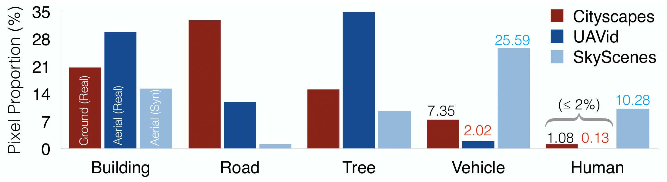
   Figure 2: Ground-View vs Aerial-View Pixel Proportions. For a subset of commonly annotated classes across Cityscapes [5] (red), UAVid [19] (dark blue) and SkyScenes (light blue), we show the percentage of pixels occupied by different classes. Aerial scenes (in UAVid) have significant under-representation of tail classes (vehicle, human). SkyScenes image curation (for the same viewpoint settings as UAVid) helps counter this discrepancy via synthetic aerial scenes.

6. Viewpoint Reproducibility: Critical to understanding how models respond to changing conditions is the ability to evaluate them under scenarios where only one variable is altered. However, any effort to do so in the real-world would be uncontrolled, due to it’s dynamic (constantly changing) nature. In contrast, simulated data allows us to do so by providing control over image generation conditions. Unlike certain existing aerial datasets that do not support this feature (see Table. 1), we do so in SkyScenes by additionally storing comprehensive metadata for each viewpoint (and image), including details about camera world coordinates, orientation and all movable / immovable actors and objects in the scene. We couple this with rigorous consistency checks for image generation that verify the number of actors, their location, sensor height, pitch, etc. This meticulous approach enables us to reproduce the same viewpoint under multiple conditions effortlessly.

7. Adequate Representation of Tail Classes: Unlike ground-view datasets, pixel distribution of classes in aerial images is substantially more long-tailed (see Fig. 2; classes with smaller object size, humans), making visual recognition tasks harder. This problem is further exacerbated by differing class distributions across synthetic and real data (see Fig. 5) – especially severe for instances of human class. To counter this, we consider structured spawning of humans to ensure adequate representation.

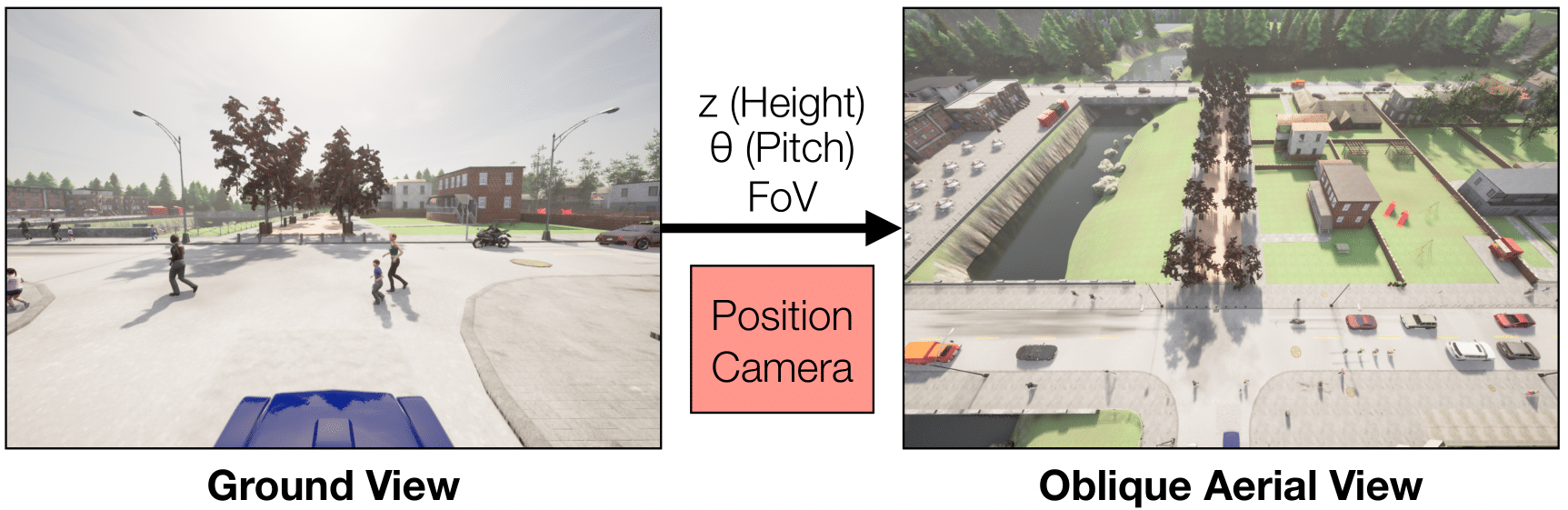
Figure 3: SkyScenes Ground View $\rightarrow$ (Oblique) Aerial View. Upon initializing a Carla [7] scene (for a Town and Variation), we re-position the camera associated with the actor to obtain oblique aerial views from ground views.

3.2 SkyScenes Image Generation

We generate SkyScenes images from Carla [7] by taking the previously mentioned considerations into account. Curating images from Carla [7] broadly consists of two key steps: (1) positioning the agent camera in an aerial perspective and (2) procedurally guiding the agent within the scene to capture images. We accomplish the first by mimicking a UAV perspective in Carla [7] by positioning the ego vehicle (with RGB, semantic and depth sensors) based on specified (high) altitude ($h$) and pitch ($\theta$) values to generate aerial views (see Fig. 3). Once positioned, the agent is translated by fixed amounts to traverse the scene and capture images from various viewpoints (detailed in Algo. 1 in the appendix). Initially, we generate $70$ datapoints for each of the $8$ town variations under ClearNoon conditions using the baseline $h=35,\theta=45^{\circ}$ setting. Subsequently, following the traversal algorithm (see Algo. 1 in the appendix), we re-generate these datapoints across $5$ weather conditions and $12$ height/pitch variations, resulting in $70\times 8\times 5\times 12=33,600$ images.

Checks and Balances. Additionally, we ensure the following checks and balances while curating SkyScenes images.

$\triangleright$ Avoiding Overly Correlated Frames for Viewpoints.

Carla [7] uses a traffic manager with a PID controller to control the egocentric vehicle based on current pose, speed, and a list of waypoints at every pre-defined time step. Curating images at every time step (or tick) results in highly correlated frames with little change in object position. Since overly correlated frames are not very useful when training models for static scene understanding, we move the camera by a fixed distance multiple times before saving a frame. This also helps with moving dynamic actors by a considerable amount in the scene. Additionally, pedestrian objects are regenerated before saving an image, which adds randomness to the spawning and placement of pedestrians and further reduces correlation between frames.

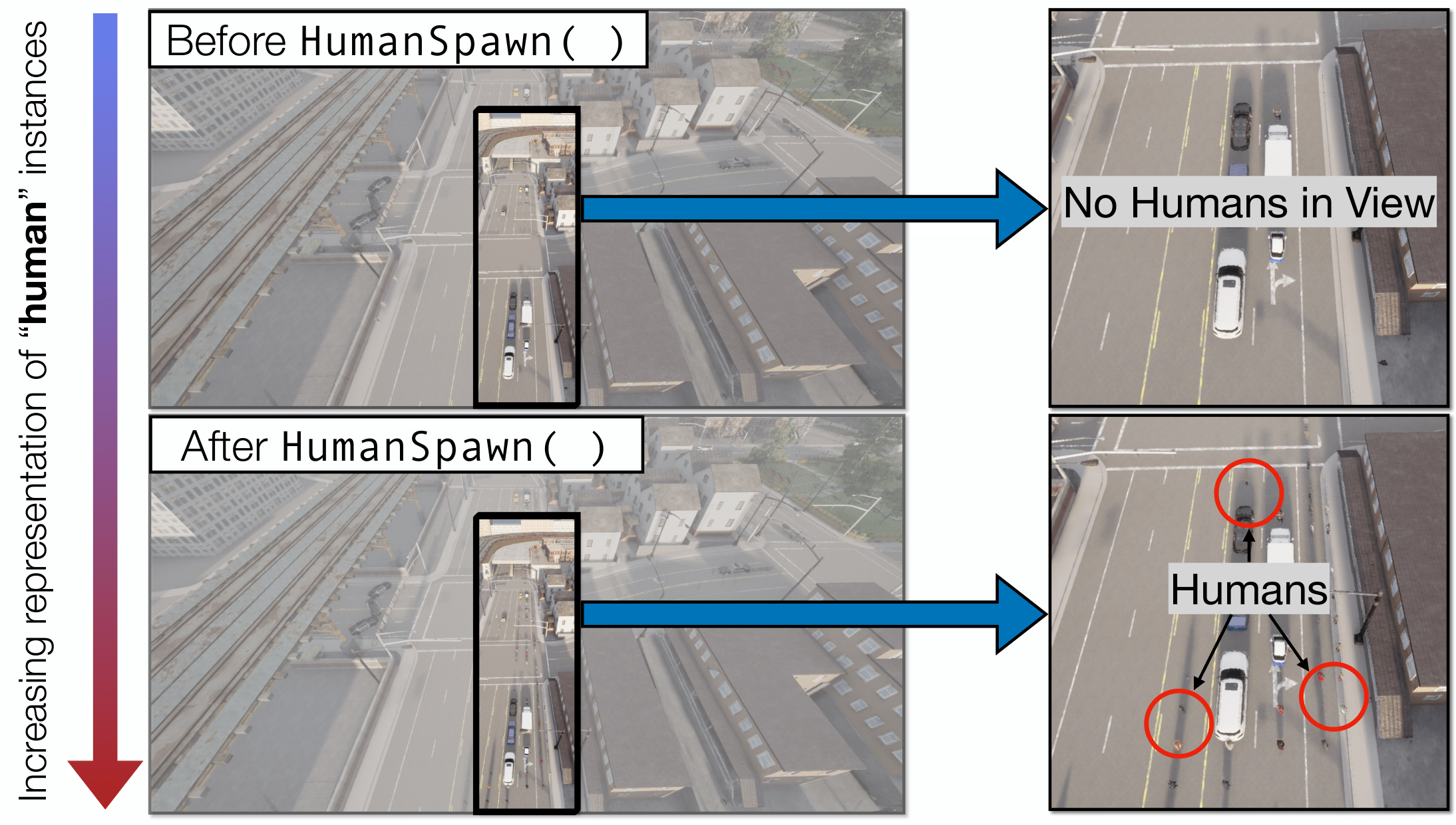
Figure 4: SkyScenes HumanSpawn() Effect. Incorporating HumanSpawn() in the image generation pipeline for SkyScenes increases the proportion of humans in snapshots ([Top]$\rightarrow$[Bottom]).

Layout	RS (%)	HS (%)
1 Town01	$0.08$	$0.14$
2 Town02	$0.18$	$0.17$
3 Town03	$0.07$	$0.21$
4 Town04	$0.14$	$0.31$
5 Town05	$0.08$	$0.43$
6 Town06	$0.07$	$0.36$
7 Town07	$0.12$	$0.26$
8 Town10HD	$0.18$	$0.35$
9 All	$0.12$	$0.28$
10 UAVid [19]	$0.13$	$0.13$

Table 2: Increase in the human representation. HumanSpawn (HS) improves the representation of humans in SkyScenes. RS = Random Spawn.

		mIoU$(\uparrow)$
Eval Data	HS	human	All
1 S		$43.03$	$80.87$
2 S	✓	61.79	84.07
3 S$\rightarrow$U		$4.71$	$45.11$
4 S$\rightarrow$U	✓	10.21	47.09

Table 3: Improved human recognition. Training on HumanSpawn (HS) SkyScenes images improves the model’s ability to recognize humans (improved mIoU). S = SkyScenes, U = UAVid [19].

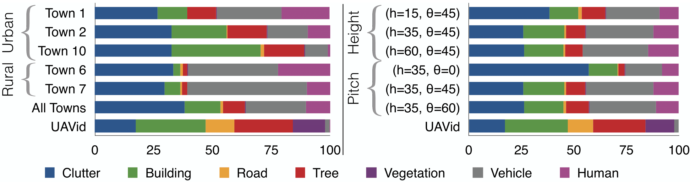
Figure 5: Class-distribution Diversity in SkyScenes. We show how the distribution of densely-annotated pixels varies across different SkyScenes conditions. [Left] Class-distribution varies substantially within and across urban and rural map layouts. [Right] Similarly, for same SkyScenes layouts (and viewpoints) class distribution varies substantially across different height and pitch values.

Figure 6: SkyScenes Per-Class Pixel Counts. We compare the number of densely annotated pixels per-class for SkyScenes (ours), Syndrone [25] (another synthetic aerial dataset) and UAVid [19] (real aerial dataset). We can see how compared to both synthetic and real counterparts, SkyScenes provides increased representation of tail classes (vehicles, humans).

$\triangleright$ Adequate Representation of humans. Real-world scenes often exhibit a long-tailed distribution in pixel proportions, particularly in aerial images where variations in object sizes and camera positions contribute to significant under-representation of the tail classes (in Fig. 2, for the shared set of classes across UAVid [19] (aerial) and Cityscapes [5] (ground), we can see that the class distributions are different and aerial images are significantly more heavy tailed). As a result, naively spawning humans (rarest class) in Carla [7] is detrimental for eventual task performance – for the human class, a SkyScenes trained DAFormer [11](with HRDA [12] source training; MiT-B5 [36] backbone) model leads to an in-distribution performance of $43.03$ mIoU and out-of-distribution (SkyScenes $\rightarrow$UAVid [19]) performance of $4.71$ mIoU. To counter this under-representation issue, we design an algorithm, HumanSpawn(), to explicitly spawn more human instances while curating SkyScenes images. HumanSpawn() increases human instances by $40-200$ per snapshot, improving the proportion of densely annotated humans in SkyScenes by approximately $10$ times (see Table. 3 & Fig. 4). This improvement in human representation is also evident in eventual task performance, with in-distribution and out-of-distribution mIoUs for humans increasing from $43.03$ to $61.79$ ($+18.76$) and $4.71$ to $10.21$ ($+5.50$) respectively (see Table. 3.)

3.3 SkyScenes: Dataset Details

Annotations. We provide semantic, instance and depth annotations for every image in SkyScenes. Semantic annotations in SkyScenes by default are across $28$ classes. These are building, fence, pedestrian, pole, roadline (markings on road), road, sidewalk, vegetation, cars, wall, traffic sign, sky, bridge, railtrack, guardrail, traffic light, water, terrain, rider, bicycle, motorcycle, bus, truck and others (see Fig. 1 for an example).

Training, Validation and Test Splits. SkyScenes has $70$ images per town (across $8$ towns) for each of the $5$ weather and daytime conditions, and $12$ height & pitch combinations, resulting in a total of $33,600$ images. We use $80$% ($26,880$ images) of the dataset for training models, with $10$% ($3,360$ images) each for validation and testing. While creating train, val and test splits, we collect equal number of samples from each town by dividing each town-specific traversal sequence into $3$ segments: the initial $80$% for training, the next $10$% for testing, and the final $10$% of the segment for validation. Moreover, within each split, we ensure that every viewpoint is accompanied by its $60$ different variations across weather, daytime, height, and pitch settings. This safeguards against any potential cross-contamination across different splits while ensuring fair representation and equal distributions of all variations.

Class Distribution(s). In Fig. 6, we compare the number of densely annotated pixels in SkyScenes with those in Syndrone [25] (another synthetic dataset) and UAVid [19] (a real aerial dataset). Compared to both the real and prior synthetic counterparts, we show that SkyScenes is specifically curated to ensure adequate tail class representation (more human and vehicle pixels) to facilitate model learning. Additionally, in Fig. 5, we highlight how the distribution of classes changes across variations within SkyScenes– rural and urban map layouts and height and pitch specifications. SkyScenes exhibits substantial diversity in class-distributions across such conditions, allowing these individual conditions to serve as diagnostic splits to assess model sensitivity (see Sec. 4.2)

4 Experiments

We conduct semantic segmentation experiments with SkyScenes to assess a few different factors. First, we check if training on SkyScenes is beneficial for real-world transfer. Second, we check if SkyScenes can augment real-world training data in low and full shot regimes. Third, we check if variations in SkyScenes can be used to assess sensitivity of trained models to changing conditions. Finally, we check if using additional modality information (depth) can help improve aerial scene understanding.

Synthetic and Real Datasets. We compare real-world generalization performance of training on SkyScenes with SynDrone [25], a recently proposed synthetic aerial dataset also curated from Carla [7]. We assess performance on $3$ real-world aerial datasets – UAVid [19], AeroScapes [22], ICG Drone [14]. Since different datasets have different class vocabularies and definitions, for our experiments, we adapt the class vocabulary of the synthetic source dataset to that of the target real-world datasets. Additionally, since different real aerial datasets have been captured from different heights and pitch angles, we train models on $(h,\theta)$ subsets of synthetic datasets that are aligned with corresponding real data $(h,\theta)$ conditions. We provide additional details for the real aligned synthetic data selection and model evaluation in Sec. D.1 of the appendix.

Models. We use both CNN – DeepLabv2 [3] (ResNet-101 [10]) – and transformer – DAFormer [11] (with HRDA [12] source training; MiT-B5 [36] backbone) – based semantic segmentation architectures for our experiments. We provide implementation details surrounding our experiments in Sec. C of the appendix.

Source	(Target) Real-World mIoU ($\uparrow$)
	UAVid	AeroScapes	ICG Drone
DeepLabv2 (R-101) [3]
1 SynDrone	$39.86$	$24.50$	$8.20$
2 SkyScenes	41.82	26.94	15.14
3 Train-on-Target	$68.53$	$68.59$	$73.12$
DAFormer (MiT-B5) [12]
4 SynDrone	$42.31$	$30.53$	$15.92$
5 SkyScenes	47.09	40.72	25.91
6 Train-on-Target	$72.47$	$77.80$	$76.44$

Table 4: Models trained on SkyScenes generalize well to the real-world. We train semantic segmentation models (DeepLabv2 [3], DAFormer [11]) on SkyScenes, SynDrone and real datasets  [25] and show how training models on SkyScenes provides better out-of-the-box generalization to multiple real-world datasets. Rows in gray represent an upper-bound oracle performance.

Source	(Target) Real-World mIoU ($\uparrow$)
	UAVid			AeroScapes			ICG Drone
	vehicle	human		vehicle	person		vehicle	person
1 SynDrone	$42.52$	$8.27$		$49.77$	$0.77$		$0.24$	$0.38$
2 SkyScenes	63.64	10.21		80.99	3.09		39.71	45.89
3 Train-on-Target	$80.70$	$41.25$		$87.58$	$57.99$		$94.08$	$83.64$

Table 5: SkyScenes training exhibits strong real-world generalization for tail classes. We show how DAFormer [11] models trained on SkyScenes exhibit improved real-world generalization compared to those trained on SynDrone for under-represented tail classes (vehicles and humans). SkyScenes training facilitates better recognition of tail class instances. Rows in gray are meant to represent oracle numbers, indicating an upper bound on attainable performance.

4.1 SkyScenes $\to$ Real Transfer

$\triangleright$ SkyScenes trained models generalize well to real-settings. In Table. 4, we show how models trained on SkyScenes exhibit strong out-of-the box generalization performance on multiple real world datasets. We find that SkyScenes pretraining exhibits stronger generalization compared to SynDrone [25] across both CNN and transformer segmentation backbones. In Table. 5, we show how generalization improvements are more pronounced for under-represented tail classes (vehicles and humans).

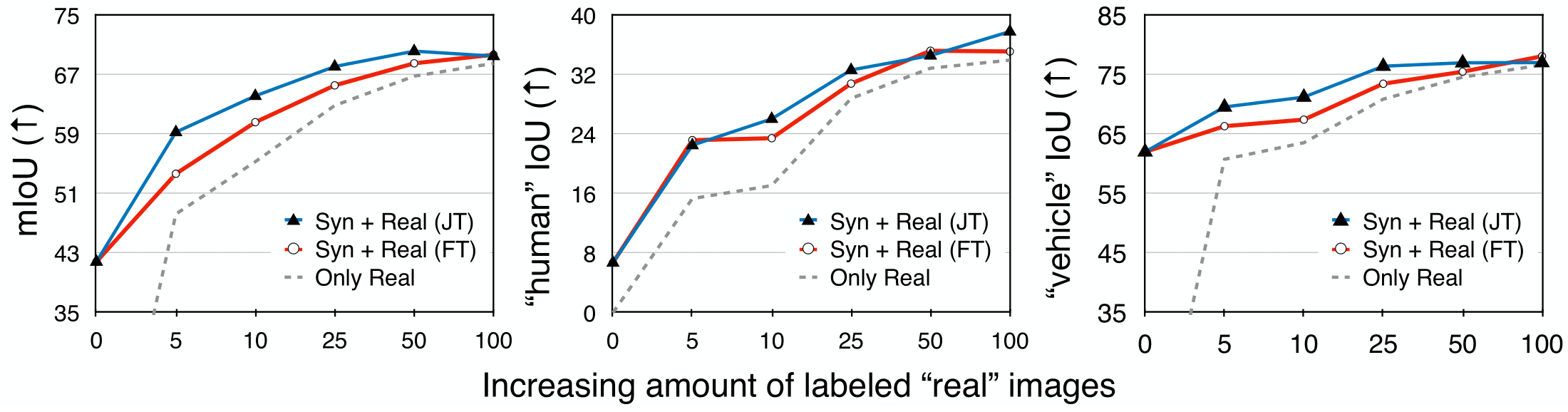
Figure 7: SkyScenes can augment “real” training data. We show how SkyScenes can additionally augment real (UAVid [19]) training data. We compare DeepLabv2 [3] models trained using only $5\%,10\%,25\%,50\%,100\%$ of labeled UAVid [19] images with counterparts that were either (1) pretrained on SkyScenes, and finetuned on UAVid [19] (FT) or (2) trained jointly on SkyScenes and UAVid [19] (JT). We find that [Left] additionally augmenting training data with SkyScenes and help improve real-world generalization in low-shot regimes, [Middle, Right] especially for under-represented classes.

$\triangleright$ SkyScenes can augment real training data. In addition to zero-shot real-world generalization, akin to other synthetic aerial datasets, we also show how SkyScenes is useful as additional training data when labeled real-world data is available. In Fig. 7, for SkyScenes $\to$UAVid [19], we compare models trained only using $5\%,10\%,25\%,50\%,100\%$ of the $200$ UAVid [19] training images with counterparts that were either pretrained using SkyScenes data or additionally supplemented with SkyScenes data at training time. We find that in low-shot regimes (when little “real” world data is available), SkyScenes data (either explicitly via joint training or implicitly via finetuning) is beneficial in improving recognition performance. We find this to be especially beneficial for under-represented classes in aerial imagery (such as humans and vehicles). We discuss more such results across other real-world datasets in Sec. D.2 of the appendix.

Train	Test mIoU ($\uparrow$)
	Clear	Cloudy	Rainy
1 Clear	$73.91$	$73.59$	$69.95$
2 Cloudy	$69.60$	$74.02$	$69.14$
3 Rainy	$69.00$	$73.36$	$72.62$

(a) Weather Variations

Train	Test mIoU ($\uparrow$)
	Noon	Sunset	Night
1 Noon	$73.91$	$71.16$	$35.60$
2 Sunset	$63.16$	$66.53$	$39.36$
3 Night	$52.00$	$57.35$	$70.36$

(b) Daytime Variations

Train	Test mIoU ($\uparrow$)
	Rural	Urban
1 Rural	$58.00$	$35.90$
2 Urban	$38.99$	$73.16$

(c) Map Variations

	Test mIoU ($\uparrow$)
Height	Pitch
	$\theta=0^{\circ}$	$\theta=45^{\circ}$	$\theta=60^{\circ}$	$\theta=90^{\circ}$
1 $h=15$m	48.50	$50.71$	$45.22$	$42.21$
2 $h=35$m	$50.49$	$55.74$	$57.11$	$52.19$
3 $h=60$m	$45.33$	$49.79$	$50.37$	$44.62$

(d) Height & Pitch Variations

Table 6: Model Sensitivity to Changing Conditions. We show how changing conditions (weather, daytime, map, viewpoint) in SkyScenes can serve as diagnostic test splits to assess the sensitivity of trained DAFormer [11] semantic segmentation models. In (a) and (b), we evaluate models trained under different weather and daytime conditions across the same conditions. In (c), we evaluate models trained on rural and urban scenes across the same layouts. In (d), we evaluate a model trained on moderate height, pitch settings ($h=35,\theta=45^{\circ}$) across different $h,\theta$ variations. We observe that, as the altitude increases, oblique viewpoints are best suited for recognition. Best numbers across each row condition is highlighted in blue.

4.2 SkyScenes as a Diagnostic Framework

As noted earlier, the images we curate in SkyScenes contain several variations – ranging from $5$ different weather and daytime conditions, rural and urban map layouts, and $12$ different height and pitch combinations (see Fig. 5 for variations in class distributions). We curate images under such diverse conditions in a controlled manner – ensuring the same spatial coordinates for $(h,\theta)$ variations, same spatial coordinates and $(h,\theta)$ settings across different weather and daytime conditions, same number of images across layouts. This allows us to assess the sensitivity of trained models to one factor of variation ($h$, $\theta$, daytime, weather, map layout) by changing that specific aspect. We summarize some takeaways from such experiments in Table. 6.

In Table. 6 (a), we show how models trained in a certain weather condition are best at generalizing to the same condition at test-time. We make similar observations for daytime variations in Table. 6 (b). In Table. 6 (c), we show how models trained in rural conditions fail to perform well in urban test-time conditions and vice-versa. In Table. 6 (d), we evaluate a model trained under moderate $(h=35,\theta=45^{\circ})$ conditions under different $(h,\theta)$ variations. We find that as altitudes increase, trained models are better at recognizing objects from oblique ($\theta\in(0^{\circ},90^{\circ})$) viewpoints. We provide exhaustive quantitative comparisons in Sec. D.3 of the appendix.

Sensors	SkyScenes Test mIoU ($\uparrow$)
	clutter	building	road	tree	low-veg.	vehicle	human	Avg
1 RGB	$87.80$	$94.54$	$94.07$	$88.03$	$69.37$	$82.89$	$43.35$	$80.01$
2 RGB+D	90.64	95.97	94.87	89.41	74.36	86.87	50.47	83.22

Table 7: Multi-modal Segmentation in SkyScenes. We show how SkyScenes enables developing multi-modal segmentation models. We evaluate M3L multimodal segmentation architectures (with MiT-B5 backbones) with RGB and RGB+D observations and show additional sensors help substantially improve aerial scene understanding. We consider the broad set of UAVid class palette for this experiment.

4.3 SkyScenes Enables Multi-modal Recognition

Sensors on UAVs in deployable settings are not limited to RGB cameras. It is common to have UAVs deployed in the real-world with additional modality sensors, such as depth. Additional sensor modalities can also potentially help improve aerial scene understanding. In Table. 7, we check if assisting RGB with Depth observations for SkyScenes viewpoints can help improve aerial semantic segmentation using M3L [20], a model capable of multimodal segmentation. Similar to our DAFormer [11] experiments, we consider a SegFormer equivalent version of M3L [20] (with an MiT-B5 [36] backbone). We test RGB and RGB+D models trained under $(h=35,\theta=45^{\circ})$ (moderate viewpoint) conditions on SkyScenes and find that incorporating additional Depth observations can substantially improve recognition performance. This demonstrates that annotated images in SkyScenes can be used to train multimodal scene-recognition models.

5 Conclusion

We introduce SkyScenes, a large-scale densely-annotated dataset of synthetic aerial scenes curated from unmanned aerial vehicle (UAV) perspectives. We collect SkyScenes images from Carla by first aerially situating an agent (to get an aerial perspective) and then procedurally tele-operating the agent through the scene to capture aerial frames with corresponding semantic, instance and depth annotations. Our careful curation process ensures that SkyScenes images are carefully curated across diverse weather, daytime, map, height and pitch conditions, with accompanying metadata that enables reproducing the same viewpoint (spatial coordinates and perspective) under differing conditions.

Through our experiments, we demonstrate how (1) SkyScenes trained models can generalize to real-world settings, (2) SkyScenes images can augment labeled real-world data in low-shot regimes, (3) SkyScenes can serve as a diagnostic framework to assess model sensitivity to changing conditions and (4) additional sensors, such as Depth, in SkyScenes can facilitate development of multi-modal aerial scene understanding models.

Lastly, we plan on updating SkyScenes with evolving considerations for real-world aerial scene-understanding – improved realism, additional anticipated edge cases – as more and more features are supported in the underlying simulator. We intend to release both the dataset and associated generation code for SkyScenes publicly, and hope that our experimental findings encourage further research using SkyScenes for aerial scenes.

Acknowledgements. We would like to thank Sean Foley for his contributions to the early efforts and discussions of this project. This work has been partially sponsored by NASA University Leadership Initiative (ULI) #80NSSC20M0161, ARL, and NSF #2144194.

Appendix A Appendix

This appendix is organized as follows. In Sec. B, we provide more details on different aspects of dataset – including the procedural image curation algorithm, algorithm to ensure appropriate representation of human instances and brief descriptions of all the classes in SkyScenes. Then, we describe experimental details in Sec. C – class-merging schemes used for our SkyScenes $\rightarrow$Real transfer experiments, train / val / test splits, experimental details for SkyScenes diagnostic setup to probe model vulnerabilities. Sec. D provides more quantitative and qualitative experimental results.

Appendix B SkyScenes Details

B.1 Image Generation Algorithms

We curate SkyScenes using Carla [7] $0.9.14$ simulator. The generation process broadly consists of two key steps: (1) positioning the agent camera in an aerial perspective and (2) procedurally guiding the agent within the scene to capture images. We accomplish the first by mimicking a UAV perspective in Carla [7] by positioning the ego vehicle (with RGB, semantic, depth and instance segmentation sensors) based on specified altitude ($h$) and pitch ($\theta$) values to generate aerial views. This also requires setting other scene information like – town, weather, and daytime. The camera $\texttt{FoV}=110^{\circ}$ (field of view) and $\{H,W\}=\{2160,1440\}$ (image resolution) are also set.

To maintain the adequate representation of tail classes, especially for humans we incorporate structured spawning of humans using Algo. 2. Carla [7] has a limit on the number of actors that can be spawned in a scene, which depends on factors such as the type and size of the town, number of lanes to spawn vehicles, and amount of sidewalk area. To overcome this limitation, we decided to bring the actors into the field of view of the camera instead of having them spread out in the scene. We developed an algorithm to find all the points to spawn pedestrians in the field of view using the camera location and spawn them like vehicles on roads. After taking a snapshot, we destroy the spawned pedestrians and repeat the process. Manual spawning not only increases the number of human instances and their proportion but also aligns their placement with real-world settings. The steps involved in manual spawning instances of humans are summarized below:

• Specify maximum number of humans to be spawned $N_{\text{max}}$

• Get camera position $(x,y,z)$, set a pre-defined distance $d$ to check for spawnable locations and execute the subroutine in Algo. 2. This will place the actors in the field of view till a junction or the next driving lane.

• If at a junction, obtain the left and the right waypoints for every retrieved location at a distance of $d$ to get the list of waypoints.

• Using the waypoint from the end of the current lane, generate waypoints for the new main, left and right lanes by repeating the previous steps.

• Repeat the above steps till $N_{\text{humans}}\leq N_{\text{max}}$

Once positioned, the agent is translated by fixed amounts to traverse the scene and capture images from various viewpoints. Initially, we generate $70$ datapoints for each of the $8$ town variations under ClearNoon conditions using the baseline $h=35,\theta=45^{\circ}$ setting. Subsequently, following the traversal algorithm (Algo. 1), we re-generate these datapoints across $5$ weather conditions and $12$ height/pitch variations, resulting in $70\times 8\times 5\times 12=33,600$ images.

Algorithm 1 SkyScenes ImgGen ($z$, $\theta$, FoV, $H$, $W$)

1:# Initialize key Carla parameters

2:Input: $z$ (height), $\theta$ (pitch), FoV, $H$, $W$

3:# Initialize auxiliary Carla parameters

4:Initialize: MB$\leftarrow$Off $\triangleright$ Turn off motion blur

5:Initialize: Post-process RGB$\leftarrow$True $\triangleright$ Turn on RGB post processing

6:Dataset: $D=\{\cdot\}$

7:# Town and variation vocabulary

8:$\mathbb{T}=\{T_{i}\}_{i=1}^{M}$ (Towns), $\mathbb{V}=\{V_{i}\}_{i=1}^{N}$ (Vars)

9:for $T_{i}\in\mathbb{T}$ do

10:     for $V_{j}\in\mathbb{V}$ do

11:         # Initialize Carla scene

12:         $E\leftarrow$Carla ${}_{\text{init}}(T_{i},V_{j})$

13:         # Position Camera

14:         Init_Sensor ($E$, $z$, $\theta$, FoV, $H$, $W$, MB)

15:         # Spawn pedestrians, vehicles, etc.

16:         Spawn_Actors ($E$)

17:         # Initialize Movement Steps

18:         $\Delta_{\text{step}}\leftarrow\Delta$, $N_{\text{steps}}\leftarrow N$

19:         for $k\in N_{\text{steps}}$ do

20:              # Sample Frame

21:              $I\leftarrow$Sample_Frame ($E$)

22:              # Get pixel-level annotations

23:              $I_{\text{anno}}\leftarrow$Get_Anno ($E$,$I$)

24:              # Get metadata

25:              $I_{\text{meta}}\leftarrow$Get_Meta ($E$,$I$)

26:              # Append to dataset

27:              $D\leftarrow D\cup\{(I,I_{\text{anno}},I_{\text{meta}})\}$

28:              # Move camera by a fixed distance

29:              Move_Camera ($E$, $\Delta_{\text{step}}$)               

30:Return: $D$ (SkyScenes data) $\triangleright$ Gathered Images

Algorithm 2 HumanSpawn ($x,y$, $d$, $p_{\text{gen}}$)

1:# Initialize parameters

2:Input: $x,y$ (camera position), $d$ (distance between spawned instances), $p_{\text{gen}}$ (spawn probability)

3:# Spawn locations

4:$D_{\text{spawn}}=\{\cdot\}$

5:# Get candidate positions in front of the camera

6:$\{(x,y)\}_{\text{front}}\leftarrow$get_loc($x$, $y$, $d$) $\triangleright$ Current Lane

7:# Get candidate positions left of camera

8:$\{(x,y)\}_{\text{left}}\leftarrow$get_loc($x-\Delta_{\text{left}}$, $y$, $d$) $\triangleright$ Left Lane

9:# Get candidate positions right of camera

10:$\{(x,y)\}_{\text{right}}\leftarrow$get_loc($x+\Delta_{\text{right}}$, $y$, $d$) $\triangleright$ Right Lane

11:$D_{\text{spawn}}\leftarrow\{(x,y)\}_{\text{front}}\cup\{(x,y)\}_{\text{left}}\cup\{(x,y)\}_{\text{right}}$

12:for $(x,y)\in D_{\text{spawn}}$ do

13:     if random()$\leq p_{\text{gen}}$ then

14:         # Spawn human

15:         spawn_human()      

B.2 Class Descriptions

We provide semantic, instance, and depth annotations for every image in SkyScenes. SkyScenes provides dense semantic annotations for $28$ classes. These are:

• unlabeled: elements/objects in the scene that have not been categorized in Carla

• other: uncategorized elements

• building: includes houses, skyscrapers, and the elements attached to them.

• fence: wood or wire assemblies that enclose an area of ground

• pedestrian: humans that walk

• pole: vertically oriented pole and its horizontal components if any

• roadline: markings on road.

• road: lanes, streets, paved areas on which cars drive

• sidewalk: parts of ground designated for pedestrians or cyclists

• vegetation: trees, hedges, all kinds of vertical vegetation (ground-level vegetation is not included here).

• cars: cars in scene

• wall: individual standing walls, not part of buildings

• traffic sign: signs installed by the state/city authority, usually for traffic regulation

• sky: open sky, including clouds and sun

• ground: any horizontal ground-level structures that does not match any other category

• bridge: the structure of the bridge

• railtrack: rail tracks that are non-drivable by cars

• guardrail: guard rails / crash barriers

• traffic light: traffic light boxes without their poles.

• static: elements in the scene and props that are immovable.

• dynamic: elements whose position is susceptible to change over time.

• water: horizontal water surfaces

• terrain: grass, ground-level vegetation, soil or sand

• rider: humans that ride/drive any kind of vehicle or mobility system

• bicycle: bicycles in scenes

• motorcycle: motorcycles in scene

• bus: buses in scenes

• truck: trucks in scenes

B.3 Depth & Instance Segmentation

We also provide depth and instance segmentation annotations along with semantic segmentation annotations. Both the depth and instance segmentation sensors are mounted alongside the RGB camera and semantic segmentation sensors. Depth is stored in the $LogarithmicDepth$ format which provides better results for closer objects. We also provide depth-aided semantic segmentation results (training details in Sec. C.3).

Appendix C Experiment Details

C.1 Class Merging Details

Syn $\rightarrow$ UAVid	UAVid	SkyScenes	SynDrone
1 clutter	clutter	unlabelled	unlabelled
		other	other
		traffic sign	traffic sign
		rail track	rail track
		guard rail	guard rail
		traffic light	traffic light
		static	static
		dynamic	dynamic
		ground	ground
		sidewalk	sidewalk
		fence	fence
		sky	sky
		bridge	bridge
		water	water
		pole	pole
2 building	building	building	building
		wall	wall
3 road	road	road	road
		roadline	roadline
4 vegetation	vegetation	vegetation	vegetation
5 low vegetation	terrain	terrain	terrain
6 person	person	pedestrian	pedestrian
		rider	rider
		motorcycle	motorcycle
		bicycle	bicycle
7 vehicle	car	car	car
		truck	truck
		bus	bus
			train

Table 8: Class merging scheme for evaluating Syn $\rightarrow$ UAVid experiments The first column is the final set of merged classes we use for Syn $\rightarrow$UAVid evaluation, the second column is the original UAVid [14] classes, the third column is the original SkyScenes classes and the last column is the original SynDrone [25] classes. Each row indicates all the classes from UAVid, SkyScenes, and SynDrone that were merged and correspond to the final Syn$\rightarrow$UAVid class in the first column

Syn $\rightarrow$ AeroScapes	AeroScapes	SkyScenes	SynDrone
1 background	background	unlabelled	unlabelled
	drone	other	other
	boat	traffic sign	traffic sign
	animal	rail track	rail track
	obstacle	guard rail	guard rail
		traffic light	traffic light
		static	static
		dynamic	dynamic
		ground	ground
		sidewalk	sidewalk
		terrain	terrain
		water	water
		pole	pole
2 bicycle	bike	bicycle	bicycle
		motorcycle	motorcycle
3 person	person	pedestrian	pedestrian
		rider	rider
4 vehicle	car	car	car
		truck	truck
		bus	bus
			train
5 vegetation	vegetation	vegetation	vegetation
6 building	construction	building	building
		wall	wall
		fence	fence
		bridge	bridge
7 road	road	road	road
		roadline	roadline
8 sky	sky	sky	sky

Table 9: Class merging scheme for evaluating Syn $\rightarrow$ AeroScapes experiments The first column is the final set of merged classes we use for Syn $\rightarrow$AeroScapes evaluation, the second column is the original AeroScapes [22] classes, the third column is the original SkyScenes classes and the last column is the original SynDrone [25] classes. Each row indicates all the classes from AeroScapes, SkyScenes, and SynDrone that were merged and correspond to the final Syn$\rightarrow$AeroScapes class in the first column

Syn $\rightarrow$ ICG Drone	ICG Drone	SkyScenes	SynDrone
1 other	obstacle	unlabelled	unlabelled
	dog	other	other
	conflicting	traffic sign	traffic sign
	ar-marker	sky	sky
	unlabelled	bridge	bridge
		gurad rail	guard rail
		traffic light	traffic light
		static	static
		dynamic	dynamic
2 fence	fence	fence	fence
3 pole	fence pole	pole	pole
4 vegetation	tree	vegetation	vegetation
	bald-tree
5 building	wall	wall	wall
	roof	building	building
	door
	window
6 water	water	water	water
	pool
7 bicycle	bicycle	bicycle	bicycle
		motorcycle	motorcycle
8 vehicle	car	car	car
		truck	truck
		bus	bus
			train
9 person	person	pedestrian	pedestrian
		rider	rider
10 paved area	paved area	ground	ground
		sidewalk	sidewalk
		road	road
		roadline	roadline
		rail track	rail track
11 terrain	rocks	terrain	terrain
	gravel
	dirt
	vegetation
	grass

Table 10: Class merging scheme for evaluating Syn $\rightarrow$ ICG Drone experiments The first column is the final set of merged classes we use for Syn $\rightarrow$ICG Drone evaluation, the second column is the original ICG Drone [14] classes, the third column is the original SkyScenes classes and the last column is the original SynDrone [25] classes. Each row indicates all the classes from ICG Drone, SkyScenes, and SynDrone that were merged and correspond to the final Syn$\rightarrow$ICG Drone class in the first column

$\triangleright$ Synthetic$\rightarrow$Real. As noted in Sec of the main paper, since different real-world datasets have different class vocabularies and definitions, for our Synthetic$\to$Real semantic segmentation experiments, we adapt the class-vocabulary of the synthetic source dataset (SkyScenes, SynDrone) to that of the target real dataset (UAVid, AeroScapes, ICG Drone). This is done using a class-merging scheme based on the class-vocabularies and after visually inspecting dataset annotations. We provide the class-merging schemes used for both SkyScenes and SynDrone [25] (synthetic) across real counterparts UAVid [19] (in Table. 8), AeroScapes [22] (in Table. 9) and ICG Drone [14] (in Table. 10).

$\triangleright$ SkyScenes Diagnostic Experiments. To assess the sensitivity of trained models to different factors – weather, time of day, height, pitch, etc.– we train models on different SkyScenes variations and evaluate them on held-out-variations. For these experiments, we recude the SkyScenes vocabulary to a reasonable subset of $20$ classes (consistent with the widely used Cityscapes [5] palette) – road, sidewalk, building, wall, fence, pole, traffic light, traffic sign, vegetation, water, sky, pedestrian, rider, cars, truck, bus, roadline, motorcycle, bicycle and an ignore class.

C.2 Training, Validation and Test Splits

C.2.1 Synthetic $\rightarrow$ Real Experiments

SkyScenes. For each $(h,\theta)$ combination, SkyScenes has a total of $2800$ datapoints (frames) which are distributed evenly across each of the $8$ town layouts and $5$ weather and daytime conditions. We use $80$% ($2240$ images) of these datapoints for training models, and remaining $10$% ($280$ images) each for validation and testing.
SynDrone. SynDrone has $3000$ images per town (across $8$ Carla towns) for each of the $3$ $(h,\theta)$ combinations, resulting in a total of $3000\times 8=24,000$ images per $(h,\theta)$ combination. We use $20,000$ of these datapoints for training models, with $4000$ kept aside for testing. The datapoints selected for training and testing are kept consistent with the one reported in SynDrone [25].

C.2.2 SkyScenes Diagnostic Experiments

Weather & Daytime Variations. For each weather variation we sample evenly across the $8$ towns and $9$ $(h,\theta)$ combinations (excluding $\theta=0^{\circ}$), resulting in a total of $70\times 9\times 8=5040$ images. We use $80$% ($4032$ images) of these for training models, and remaining $10$% ($504$ images) each for validation and testing. We evaluate the model on the same weather variation it was trained on and select the model with the best mIoU score for further evaluations on other weather variations.
Town Variations. For each variation in town we sample evenly across $5$ weather and daytime conditions and $9$ height and pitch variations(excluding pitch=$0^{\circ}$ variations), resulting in a total of $70\times 5\times 9=3150$ images per town variation. Out of these, $80$% ($2520$ images) is allocated for training models, with $10$% ($315$ images) each for validation and testing. We evaluate the model on the same town variation it was trained on and select the model with the best mIoU score for further evaluations on other town variations.
Height & Pitch Variations. For each $(h,\theta)$ variation, we evenly sample across $8$ towns and $5$ weather and daytime conditions, resulting in a total of $70\times 8\times 5=2800$ images per height and pitch variation. Out of these, $80$% ($2240$ images) are allocated for training models, and $10$% ($280$ images) each for validation and testing.We evaluate the model on the same height & pitch setting it was trained on and select the model with the best mIoU score for further evaluations on other height & pitch settings.

C.3 Training Details

Semantic Segmentation. For our semantic segmentation experiments we use both CNN – DeepLabv2 [3] (ResNet-101 [10] backbone) – and vision transformer – DAFormer [11] (with HRDA [12] source training; MiT-B5 [36] backbone) – based semantic segmentation architectures. Note that we utilize only the DAFormer architecture to perform source-only training for our experiments. Following [13], we enable rare class sampling  [11] and use Imagenet feature-distance for our thing classes during training. All models are trained using the AdamW [18] optimizer coupled with a polynomial learning rate scheduler with an initial learning rate of $6\times 10^{-5}$. Each model is trained for $40$k iterations with a batch size of $4$. For our fine-tuning experiments, we use an initial learning rate of $6\times 10^{-6}$.

Depth-Aided Semantic Segmentation. For our depth-aided semantic segmentation experiments in Sec. 4.3 of the main paper, similar to DAFormer [11], we employ a SegFormer [36] equivalent version of M3L [20] (multimodal segmentation network) with an MiT-B5 [36] backbone. We initialize the network with ImageNet-1k pre-trained checkpoints. For M3L Linear Fusion, we use $\alpha=0.8$. We use AdamW [15] optimizer and train on a batch size of $4$ for $50$ epochs. We use a learning rate of $10^{-4}$ for the encoder and $3\times 10^{-4}$ for the decoder with a momentum of $0.9$ and weight decay of $10^{-4}$. We set the polynomial decay of power $0.9$. We train both RGB and RGB+D models with complete supervision for $(h=35,\theta=45^{\circ})$ (moderate viewpoint) conditions on SkyScenes.

C.4 Evaluation Details

Due to memory constraints, in addition to heavily parameterized models, our GPUs were unable to fit images larger than $1280\times 720$. Hence for high-resolution datasets like UAVid, we use the trained model to make separate predictions on $4$ equally sized slightly-overlapping crops (overlap of $20$ pixels) of the of the real image and stitch crop predictions to obtain the overall image prediction. Similarly, for ICG Drone, we obtain overall image prediction using such crop predictions.

Appendix D Results

D.1 Synthetic$\to$Real Aligned Data Selection

As stated in the main paper, for our Synthetic$\to$Real experiments, we train models on $(h,\theta)$ subsets of synthetic datasets that are aligned with corresponding real data $(h,\theta)$ conditions. In case of UAVid and AeroScapes we find that $(h=35m,\theta=45^{\circ})$ viewpoints in SkyScenes and $(h=20m,\theta=30^{\circ})$ viewpoints in SynDrone are best aligned with UAVid conditions (see Table. 11 and Table. 12) and provide best transfer performance. Similarly, for ICG Drone we observe that $(h=15m,\theta=90^{\circ})$ SkyScenes conditions are best aligned with the low-altitude, nadir perspective imagery in ICG Drone and lead to best transfer performance (see Table. 13). However, for SynDrone, we find that the model trained on $(h=80m,\theta=90^{\circ})$ has best transfer performance, indicating that model performance is more sensitive to pitch alignment than height alignment.

h(m)	$\bm{\theta(^{\circ})}$	Synthetic$\rightarrow\textsc{UAV}\textnormal{id}$ mIoU ($\uparrow$)
		Clutter	Building	Road	Tree	Low Vegetation	Human	Vehicle	Avg
SkyScenes
1 $15$	$0$	$30.23$	$70.24$	$43.91$	$52.20$	$6.24$	$10.33$	$43.45$	$36.66$
2 $15$	$45$	$23.36$	$61.88$	$43.10$	$38.18$	$11.79$	$0.32$	$3.76$	$26.05$
3 $15$	$60$	$22.15$	$57.85$	$39.31$	$38.43$	$5.35$	$0.27$	$3.72$	$23.35$
4 $15$	$90$	$27.01$	$68.40$	$41.92$	$53.79$	$17.95$	$17.26$	$42.80$	$38.45$
5 $35$	$0$	$31.66$	$72.37$	$38.65$	$45.73$	$12.97$	$0.45$	$23.63$	$32.21$
6 $35$	$45$	$36.44$	$81.3$	$52.09$	$60.00$	$25.96$	$10.21$	$63.64$	$\bm{47.09}$
7 $35$	$60$	$28.17$	$68.31$	$44.96$	$44.84$	$15.32$	$0.05$	$8.81$	$30.06$
8 $35$	$90$	$28.88$	$76.49$	$48.11$	$57.88$	$13.61$	$7.98$	$49.32$	$40.07$
9 $60$	$0$	$24.83$	$66.37$	$26.18$	$39.58$	$11.43$	$0.01$	$4.76$	$24.74$
10 $60$	$45$	$27.32$	$66.02$	$38.29$	$41.45$	$11.72$	$0.0$	$5.25$	$27.15$
11 $60$	$60$	$23.98$	$62.62$	$32.72$	$41.00$	$17.55$	$0.00$	$6.34$	$26.32$
12 $60$	$90$	$28.84$	$75.03$	$40.72$	$54.27$	$13.02$	$1.16$	$49.48$	$37.50$
SynDrone
13 $20$	$30$	$36.20$	$75.74$	$48.71$	$55.95$	$28.75$	$8.27$	$42.52$	$\underline{42.31}$
14 $50$	$60$	$31.13$	$69.93$	$48.87$	$54.49$	$27.71$	$1.32$	$36.06$	$38.50$
15 $80$	$90$	$28.89$	$65.66$	$42.05$	$51.51$	$32.16$	$0.13$	$28.39$	$35.54$

Table 11: Models trained on UAVid aligned (h,$\bm{\theta}$) display better generalization performance . We have trained both SkyScenes and SynDrone on every subset of (h,$\theta$) provided by the respective datasets

h(m)	$\bm{\theta(^{\circ})}$	Synthetic$\rightarrow\textsc{AeroScapes}$ mIoU ($\uparrow$)
		Background	Bicycle	Person	Vehicle	Vegetation	Building	Road	Sky	Avg
SkyScenes
1 $15$	$0$	$32.39$	$0.00$	$3.45$	$55.42$	$56.08$	$30.11$	$15.4$	$69.75$	$32.81$
2 $15$	$45$	$25.26$	$0.0$	$4.12$	$5.72$	$31.9$	$11.56$	$26.43$	$7.23$	$14.03$
3 $15$	$60$	$27.16$	$0.00$	$1.69$	$11.81$	$32.27$	$22.48$	$31.22$	$0.21$	$15.86$
4 $15$	$90$	$28.53$	$1.32$	$30.35$	$77.22$	$53.09$	$12.09$	$11.43$	$0.00$	$26.75$
5 $35$	$0$	$32.45$	$0.00$	$0.00$	$17.65$	$51.00$	$42.03$	$7.14$	$75.03$	$28.16$
6 $35$	$45$	$32.07$	$0.8$	$3.09$	$80.99$	$51.34$	$45.54$	$23.64$	$88.29$	$\bm{40.72}$
7 $35$	$60$	$29.72$	$0.00$	$0.00$	$30.00$	$45.54$	$24.01$	$23.26$	$0.00$	$19.07$
8 $35$	$90$	$30.62$	$1.9$	$2.62$	$72.77$	$55.56$	$26.85$	$17.34$	$1.94$	$26.2$
9 $60$	$0$	$29.99$	$0.0$	$0.0$	$1.05$	$34.68$	$42.11$	$10.53$	$49.63$	$21.00$
10 $60$	$45$	$28.05$	$0.0$	$0.0$	$7.14$	$40.60$	$22.38$	$17.84$	$5.16$	$15.15$
11 $60$	$60$	$26.71$	$0.0$	$0.0$	$0.53$	$37.93$	$19.95$	$18.63$	$0.80$	$13.07$
12 $60$	$90$	$31.08$	$0.00$	$0.11$	$30.83$	$58.10$	$31.61$	$17.76$	$0.06$	$21.19$
SynDrone
13 $20$	$30$	$32.32$	$0.92$	$0.77$	$49.77$	$54.42$	$35.71$	$6.89$	$63.45$	$\underline{30.53}$
14 $50$	$60$	$32.29$	$0.99$	$0.05$	$29.41$	$56.47$	$39.59$	$22.15$	$5.36$	$23.29$
15 $80$	$90$	$30.40$	$0.09$	$0.01$	$27.09$	$51.04$	$39.20$	$27.32$	$0.17$	$21.92$

Table 12: Models trained on AeroScapes aligned (h,$\bm{\theta}$) display better generalization performance . We have trained both SkyScenes and SynDrone on every subset of (h,$\theta$) provided by the respective datasets

h(m)	$\bm{\theta(^{\circ})}$	Synthetic$\rightarrow\textsc{ICG Drone}$ mIoU ($\uparrow$)
		other	fence	pole	vegetation	building	water	bicycle	vehicle	person	paved area	terrain	Avg	Avg∗
SkyScenes
1 $15$	$0$	$2.85$	$0.28$	$0.04$	$6.60$	$29.94$	$0.83$	$0.06$	$0.45$	$0.35$	$27.46$	$0.72$	$6.33$	$7.33$
2 $15$	$45$	$2.87$	$0.67$	$0.21$	$6.91$	$32.12$	$3.25$	$0.49$	$5.03$	$25.22$	$56.69$	$8.78$	$12.93$	$14.51$
3 $15$	$60$	$3.98$	$0.00$	$0.73$	$5.19$	$35.85$	$0.66$	$0.12$	$4.95$	$3.56$	$57.51$	$1.21$	$10.34$	$12.06$
4 $15$	$90$	$3.74$	$1.45$	$2.51$	$6.67$	$46.72$	$8.19$	$2.21$	$39.71$	$45.89$	$79.84$	$6.04$	$\bm{22.09}$	$\bm{25.91}$
5 $35$	$0$	$1.63$	$0.00$	$0.06$	$4.86$	$28.84$	$2.77$	$0.07$	$0.04$	$0.30$	$29.70$	$6.96$	$6.84$	$7.40$
6 $35$	$45$	$4.37$	$0.39$	$1.60$	$4.90$	$25.33$	$4.98$	$0.10$	$1.35$	$0.29$	$68.37$	$29.51$	$12.83$	$11.92$
7 $35$	$60$	$2.06$	$0.01$	$0.04$	$6.15$	$30.05$	$9.43$	$0.02$	$0.23$	$0.11$	$54.99$	$13.43$	$10.59$	$11.23$
8 $35$	$90$	$2.13$	$0.04$	$0.64$	$7.34$	$28.07$	$7.26$	$0.09$	$0.30$	$0.11$	$50.27$	$11.11$	$9.76$	$9.63$
9 $60$	$0$	$2.23$	$0.00$	$0.00$	$8.30$	$32.07$	$1.72$	$0.10$	$0.03$	$0.17$	$11.58$	$13.30$	$6.32$	$6.00$
10 $60$	$45$	$1.07$	$0.00$	$0.02$	$7.71$	$30.03$	$4.73$	$0.17$	$0.00$	$0.22$	$31.62$	$8.87$	$7.68$	$8.28$
11 $60$	$60$	$0.81$	$0.00$	$0.02$	$4.84$	$26.59$	$7.21$	$0.16$	$0.01$	$0.16$	$51.34$	$8.39$	$9.05$	$9.11$
12 $60$	$90$	$1.32$	$0.00$	$0.25$	$7.90$	$27.64$	$3.21$	$0.04$	$0.26$	$0.22$	$21.36$	$6.65$	$6.26$	$6.76$
SynDrone
13 $20$	$30$	$6.50$	$0.10$	$1.47$	$5.47$	$27.68$	$16.07$	$0.29$	$11.89$	$0.30$	$62.47$	$32.97$	$15.02$	$13.97$
14 $50$	$60$	$5.88$	$0.05$	$0.45$	$4.70$	$36.85$	$31.48$	$0.09$	$0.38$	$0.44$	$64.83$	$29.13$	$15.84$	$15.47$
15 $80$	$90$	$4.17$	$0.01$	$0.25$	$0.67$	$37.34$	$36.11$	$0.04$	$0.24$	$0.38$	$68.21$	$41.85$	$\underline{17.75}$	$\underline{15.92}$

Table 13: Models trained on ICG Drone aligned (h,$\bm{\theta}$) display better generalization performance . We have trained both SkyScenes and SynDrone on every subset of (h,$\theta$) provided by the respective datasets. Avg^∗ - Average IoU reported over all classes excluding other and terrain(both numbers are reported since a discrepancy was observed in other and terrain class from SkyScenes which resulted in overlapping cases across these classes)

Training	Data Size	Synthetic$\rightarrow\textsc{UAV}\textnormal{id}$ mIoU ($\uparrow$)
		Clutter	Building	Road	Tree	Low Vegetation	Human	Vehicle	Avg
SkyScenes
1 FT	$5\%$	$47.60$	$83.73$	$62.08$	$58.98$	$33.70$	$23.21$	$66.36$	53.67
2 FT	$10\%$	$50.06$	$86.93$	$67.70$	$70.58$	$58.09$	$23.47$	$67.46$	60.61
3 FT	$25\%$	$57.61$	$89.37$	$73.28$	$73.30$	$61.15$	$30.82$	$73.50$	65.57
4 FT	$50\%$	$62.44$	$90.87$	$75.84$	$74.75$	$65.16$	$35.24$	$75.52$	68.54
5 FT	$100\%$	$63.56$	$91.23$	$77.03$	$76.01$	$66.81$	$35.14$	$78.12$	69.70
6 JT	$5\%$	$52.09$	$86.83$	$65.35$	$68.45$	$50.06$	$22.53$	$69.59$	59.27
7 JT	$10\%$	$56.23$	$89.06$	$71.84$	$73.23$	$61.35$	$26.07$	$71.25$	64.15
8 JT	$25\%$	$61.50$	$90.45$	$75.98$	$75.18$	$64.56$	$32.65$	$76.45$	68.11
9 JT	$50\%$	$65.70$	$91.68$	$78.14$	$76.84$	$67.29$	$34.59$	$77.02$	70.18
10 JT	$100\%$	$64.19$	$89.06$	$74.52$	$76.59$	$67.34$	$37.82$	$77.06$	$\underline{69.51}$
SynDrone
11 FT	$5\%$	$46.58$	$82.81$	$59.69$	$58.95$	$37.53$	$21.50$	$63.78$	$52.97$
12 FT	$10\%$	$48.08$	$85.76$	$64.56$	$69.14$	$54.29$	$21.91$	$65.94$	$58.53$
13 FT	$25\%$	$56.46$	$88.78$	$70.97$	$72.06$	$61.14$	$28.59$	$73.12$	$64.45$
14 FT	$50\%$	$61.70$	$90.45$	$73.83$	$75.48$	$64.67$	$33.45$	$74.98$	$67.79$
15 FT	$100\%$	$63.42$	$91.16$	$75.75$	$76.56$	$66.63$	$33.53$	$76.59$	$69.10$
16 JT	$5\%$	$49.72$	$81.39$	$63.63$	$65.52$	$49.00$	$6.70$	$70.19$	$55.17$
17 JT	$10\%$	$52.94$	$85.41$	$67.25$	$71.47$	$59.05$	$23.32$	$72.43$	$61.70$
18 JT	$25\%$	$59.99$	$87.79$	$72.26$	$74.00$	$65.59$	$36.32$	$75.91$	$67.40$
19 JT	$50\%$	$63.38$	$88.88$	$74.09$	$74.97$	$66.85$	$38.47$	$77.45$	$69.16$
20 JT	$100\%$	$64.06$	$89.09$	$74.61$	$75.98$	$67.31$	$40.59$	$78.40$	70.01
Target
21 Target	$5\%$	$41.36$	$80.24$	$57.07$	$57.20$	$25.72$	$15.35$	$60.79$	$48.25$
22 Target	$10\%$	$42.94$	$81.50$	$61.06$	$67.51$	$53.32$	$17.10$	$63.58$	$55.29$
23 Target	$25\%$	$53.57$	$86.89$	$69.70$	$70.95$	$59.22$	$28.82$	$70.91$	$62.86$
24 Target	$50\%$	$59.75$	$89.42$	$72.58$	$74.28$	$64.09$	$32.89$	$74.61$	$66.81$
25 Target	$100\%$	$62.45$	$90.76$	$74.41$	$75.83$	$65.65$	$33.97$	$76.65$	$68.53$

(a) [DeepLabv2 UAVid ]

Training	Data Size	Synthetic$\rightarrow\textsc{UAV}\textnormal{id}$ mIoU ($\uparrow$)
		Clutter	Building	Road	Tree	Low Vegetation	Human	Vehicle	Avg
SkyScenes
1 FT	$5\%$	$52.63$	$88.02$	$67.74$	$66.56$	$49.14$	$29.53$	$72.68$	$60.90$
2 FT	$10\%$	$57.43$	$89.48$	$72.93$	$74.26$	$61.96$	$35.89$	$75.61$	$66.79$
3 FT	$25\%$	$63.43$	$90.87$	$78.66$	$75.59$	$64.94$	$40.29$	$79.05$	$70.41$
4 FT	$50\%$	$67.06$	$92.22$	$79.76$	$77.86$	$68.97$	$41.90$	$80.64$	$72.63$
5 FT	$100\%$	$67.67$	$92.51$	$79.66$	$78.68$	$69.03$	$42.29$	$81.27$	$73.02$
6 JT	$5\%$	$53.72$	$85.99$	$66.35$	$69.02$	$56.45$	$35.82$	$73.51$	62.97
7 JT	$10\%$	$59.77$	$87.82$	$72.97$	$74.68$	$64.95$	$37.63$	$75.21$	67.58
8 JT	$25\%$	$63.58$	$88.68$	$76.22$	$75.80$	$67.49$	$41.17$	$78.43$	70.20
9 JT	$50\%$	$66.83$	$89.63$	$77.76$	$76.90$	$68.45$	$43.79$	$79.41$	71.83
10 JT	$100\%$	$66.92$	$89.74$	$76.89$	$77.98$	$68.81$	$45.32$	$80.06$	$72.25$
SynDrone
11 FT	$5\%$	$53.53$	$87.81$	$67.31$	$67.51$	$55.40$	$33.94$	$73.40$	$62.70$
12 FT	$10\%$	$56.80$	$89.64$	$72.31$	$74.22$	$64.12$	$36.77$	$75.15$	$67.00$
13 FT	$25\%$	$63.77$	$91.11$	$78.18$	$76.17$	$66.63$	$41.27$	$78.90$	$70.86$
14 FT	$50\%$	$66.89$	$92.06$	$79.14$	$77.79$	$69.22$	$43.32$	$80.47$	$72.70$
15 FT	$100\%$	$67.48$	$92.48$	$79.48$	$78.76$	$69.73$	$42.82$	$81.57$	$73.19$
16 JT	$5\%$	$53.54$	$85.58$	$64.30$	$70.07$	$58.64$	$29.86$	$73.21$	$62.17$
17 JT	$10\%$	$58.00$	$87.26$	$71.23$	$74.57$	$64.65$	$35.58$	$75.08$	$66.62$
18 JT	$25\%$	$61.82$	$88.35$	$74.09$	$75.38$	$66.43$	$40.85$	$78.21$	$69.31$
19 JT	$50\%$	$65.10$	$89.19$	$75.80$	$76.95$	$68.15$	$40.65$	$78.52$	$70.62$
20 JT	$100\%$	$66.78$	$89.81$	$76.56$	$77.91$	$69.38$	$45.34$	$80.45$	$72.32$
Target
21 Target	$5\%$	$51.20$	$86.59$	$62.68$	$66.73$	$50.46$	$34.50$	$71.97$	$60.59$
22 Target	$10\%$	$53.95$	$88.35$	$70.56$	$73.65$	$63.29$	$35.50$	$74.12$	$65.63$
23 Target	$25\%$	$62.86$	$90.48$	$76.89$	$76.02$	$66.66$	$41.03$	$78.31$	$70.31$
24 Target	$50\%$	$66.23$	$91.84$	$78.75$	$77.61$	$68.44$	$42.36$	$79.90$	$72.16$
25 Target	$100\%$	$66.67$	$92.20$	$79.16$	$78.35$	$68.93$	$41.25$	$80.70$	$72.47$

(b) [DAFormer UAVid ]

Training	Data Size	Synthetic$\rightarrow\textsc{AeroScapes}$ mIoU ($\uparrow$)
		Background	Bicycle	Person	Vehicle	Vegetation	Building	Road	Sky	Avg
SkyScenes
1 FT	$5\%$	$59.25$	$4.69$	$43.11$	$80.81$	$91.79$	$59.32$	$72.43$	$89.13$	62.57
2 FT	$10\%$	$71.45$	$14.76$	$47.53$	$82.43$	$92.96$	$60.08$	$83.92$	$93.09$	68.28
3 FT	$25\%$	$72.93$	$21.78$	$47.80$	$81.69$	$93.42$	$62.25$	$84.51$	$94.30$	69.84
4 FT	$50\%$	$76.15$	$23.69$	$53.11$	$84.45$	$93.58$	$67.00$	$87.73$	$94.06$	72.47
5 FT	$100\%$	$76.91$	$25.30$	$53.07$	$82.27$	$94.05$	$67.81$	$87.78$	$94.51$	72.71
6 JT	$5\%$	$67.86$	$22.42$	$46.63$	$87.18$	$92.11$	$59.69$	$85.04$	$92.31$	69.16
7 JT	$10\%$	$76.24$	$30.44$	$56.33$	$83.67$	$92.15$	$69.39$	$89.70$	$94.86$	74.10
8 JT	$25\%$	$76.33$	$34.14$	$53.50$	$87.87$	$93.12$	$68.89$	$90.23$	$95.23$	74.91
9 JT	$50\%$	$78.13$	$32.06$	$57.32$	$87.52$	$93.23$	$73.14$	$90.42$	$94.69$	$\underline{75.81}$
10 JT	$100\%$	$80.35$	$32.43$	$60.14$	$87.98$	$94.00$	$75.20$	$91.89$	$95.06$	77.13
SynDrone
11 FT	$5\%$	$57.20$	$3.79$	$39.07$	$77.44$	$90.79$	$58.60$	$69.09$	$88.48$	$60.56$
12 FT	$10\%$	$69.18$	$14.77$	$47.07$	$64.87$	$92.29$	$60.42$	$81.09$	$91.94$	$65.20$
13 FT	$25\%$	$72.21$	$23.27$	$44.35$	$79.72$	$92.83$	$63.94$	$83.31$	$92.31$	$68.99$
14 FT	$50\%$	$74.28$	$22.32$	$49.59$	$81.59$	$93.01$	$64.70$	$85.56$	$92.81$	$70.49$
15 FT	$100\%$	$74.61$	$22.45$	$49.13$	$81.42$	$93.15$	$64.18$	$86.15$	$92.64$	$70.47$
16 JT	$5\%$	$63.05$	$23.34$	$46.50$	$83.30$	$92.24$	$64.15$	$78.81$	$93.64$	$68.12$
17 JT	$10\%$	$74.54$	$26.14$	$53.81$	$81.26$	$93.01$	$66.44$	$88.83$	$94.62$	$72.32$
18 JT	$25\%$	$76.96$	$33.69$	$55.34$	$83.53$	$93.67$	$69.00$	$90.37$	$95.26$	$74.73$
19 JT	$50\%$	$79.35$	$31.45$	$59.18$	$85.80$	$93.66$	$74.00$	$91.27$	$95.05$	76.22
20 JT	$100\%$	$79.66$	$31.82$	$58.71$	$86.87$	$93.75$	$74.65$	$91.95$	$94.20$	$76.45$
Target
21 Target	$5\%$	$53.92$	$7.33$	$38.25$	$72.41$	$90.15$	$53.49$	$66.79$	$87.95$	$58.79$
22 Target	$10\%$	$67.08$	$14.89$	$39.79$	$63.76$	$91.65$	$58.98$	$79.45$	$91.70$	$63.41$
23 Target	$25\%$	$70.51$	$20.69$	$39.46$	$76.20$	$92.34$	$62.25$	$82.51$	$92.56$	$67.07$
24 Target	$50\%$	$73.10$	$20.95$	$45.23$	$79.07$	$92.68$	$64.70$	$84.48$	$92.11$	$69.04$
25 Target	$100\%$	$73.21$	$19.21$	$44.79$	$78.44$	$92.95$	$63.49$	$85.34$	$91.27$	$68.59$

(c) [DeepLabv2 AeroScapes ]

Training	Data Size	Synthetic$\rightarrow\textsc{AeroScapes}$ mIoU ($\uparrow$)
		Background	Bicycle	Person	Vehicle	Vegetation	Building	Road	Sky	Avg
SkyScenes
1 FT	$5\%$	$66.93$	$28.05$	$46.63$	$84.56$	$93.29$	$64.03$	$79.76$	$95.41$	$69.83$
2 FT	$10\%$	$76.11$	$31.60$	$53.95$	$88.26$	$93.92$	$67.90$	$88.45$	$96.25$	$74.56$
3 FT	$25\%$	$79.68$	$39.95$	$54.07$	$86.18$	$94.22$	$71.31$	$91.53$	$95.66$	76.56
4 FT	$50\%$	$81.09$	$39.03$	$58.80$	$86.25$	$94.42$	$76.20$	$91.15$	$96.45$	77.93
5 FT	$100\%$	$81.78$	$41.22$	$59.06$	$85.93$	$94.62$	$76.06$	$91.47$	$96.40$	78.31
6 JT	$5\%$	$69.98$	$33.78$	$50.09$	$85.72$	$93.94$	$64.09$	$82.32$	$95.64$	71.94
7 JT	$10\%$	$78.47$	$38.45$	$57.73$	$88.98$	$94.39$	$67.87$	$90.23$	$96.14$	76.53
8 JT	$25\%$	$81.07$	$40.95$	$53.79$	$88.60$	$94.30$	$71.92$	$92.76$	$95.77$	$77.39$
9 JT	$50\%$	$81.55$	$39.43$	$64.25$	$89.16$	$94.30$	$76.81$	$91.34$	$96.30$	$79.14$
10 JT	$100\%$	$83.13$	$44.90$	$60.14$	$89.55$	$94.93$	$79.55$	$92.49$	$95.83$	80.06
SynDrone
11 FT	$5\%$	$70.94$	$29.02$	$47.17$	$82.25$	$93.23$	$64.19$	$83.31$	$93.27$	$70.42$
12 FT	$10\%$	$76.62$	$29.13$	$60.31$	$86.91$	$93.80$	$66.29$	$89.80$	$95.65$	$74.81$
13 FT	$25\%$	$78.97$	$34.86$	$57.69$	$86.06$	$93.83$	$69.73$	$92.03$	$95.33$	$76.06$
14 FT	$50\%$	$80.28$	$34.42$	$63.33$	$85.34$	$94.31$	$73.71$	$91.55$	$95.69$	$77.33$
15 FT	$100\%$	$80.90$	$35.47$	$62.18$	$85.43$	$94.45$	$74.45$	$92.12$	$95.76$	$77.59$
16 JT	$5\%$	$69.12$	$30.82$	$53.16$	$81.33$	$93.19$	$61.11$	$83.80$	$95.36$	$70.99$
17 JT	$10\%$	$77.38$	$40.42$	$57.80$	$88.32$	$94.14$	$68.06$	$90.24$	$95.60$	$76.47$
18 JT	$25\%$	$80.64$	$44.19$	$53.95$	$89.80$	$94.28$	$71.89$	$92.58$	$96.14$	$77.94$
19 JT	$50\%$	$81.82$	$40.86$	$63.15$	$89.20$	$94.38$	$77.72$	$92.29$	$96.43$	$79.42$
20 JT	$100\%$	$79.38$	$35.85$	$50.91$	$86.01$	$94.08$	$70.88$	$90.73$	$94.32$	$75.27$
Target
21 Target	$5\%$	$66.26$	$24.03$	$47.34$	$81.04$	$92.88$	$58.85$	$78.11$	$90.85$	$67.42$
22 Target	$10\%$	$74.91$	$32.00$	$52.74$	$82.18$	$93.62$	$59.63$	$88.73$	$94.00$	$72.23$
23 Target	$25\%$	$78.16$	$41.22$	$53.29$	$84.76$	$93.95$	$66.04$	$90.92$	$95.28$	$75.45$
24 Target	$50\%$	$80.09$	$38.73$	$58.11$	$84.89$	$94.14$	$73.72$	$90.85$	$95.61$	$77.02$
25 Target	$100\%$	$80.35$	$42.65$	$57.99$	$87.58$	$94.48$	$72.65$	$91.20$	$95.51$	$77.80$

(d) [DAFormer AeroScapes ]

Table 14: SkyScenes can augment “real” training data. We compare SkyScenes against SynDrone for their ability to augment real training data. We compare DAFormer [11] and DeepLabv2 [3] models trained using only $5\%,10\%,25\%,50\%,100\%$ of labeled real dataset images (UAVid [19] and AeroScapes [22]) with counterparts that were either (1) pretrained on SkyScenes/SynDrone, and finetuned on real dataset images (FT) or (2) trained jointly on SkyScenes/SynDrone and real dataset images (JT). We find that both FT and JT with SkyScenes outperforms or is on par with SynDrone in almost all of the different labeled data splits.

D.2 SkyScenes $+$ Real Data Experiments

In addition to zero-shot transfer to real data, we also show how SkyScenes is useful as additional training data when labeled real-world data is available. In Fig. 8 and Fig. 9, we compare the performance of DeepLabv2 [3] for SkyScenes $\to$UAVid [19] and for SkyScenes $\to$AeroScapes [22] trained only using $5\%,10\%,25\%,50\%,100\%$ of UAVid [19] and AeroScapes [22] training images respectively with counterparts that were either pretrained using SkyScenes data or additionally supplemented with SkyScenes data at training time. In Fig. 10 and Fig. 11 we make a similar comparison with the DAFormer [11] architecture. In low-shot regimes (when little “real” world data is available), SkyScenes data (either explicitly via joint training or implicitly via finetuning) is beneficial in improving recognition performance. We find this to be especially beneficial for under-represented classes in aerial imagery (such as humans and vehicles). In Table. 14(a) and Table. 14(c) we present similar fine-grained (per-class) comparison of SkyScenes with SynDrone for a DeepLabv2 model when real data is available for training – via Target-Only, Finetuning or Joint-Training. Tables. 14(b) and 14(d) show similar comparisons using the DAFormer [11] model.

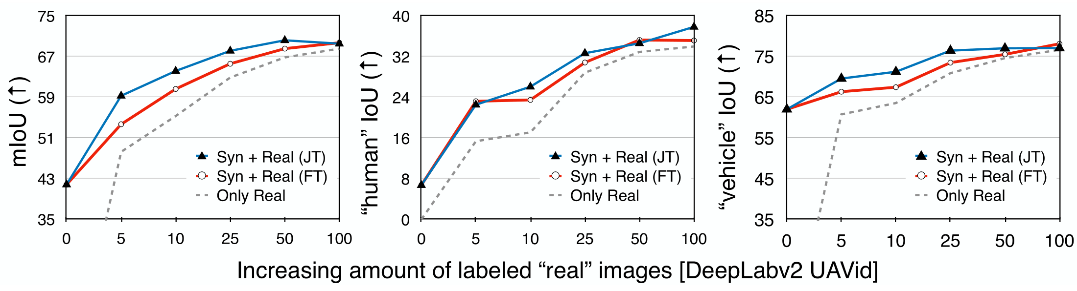
Figure 8: [DeepLabv2 UAVid] SkyScenes can augment “real” training data. We show how SkyScenes can additionally augment real (UAVid [19]) training data. We compare DeepLabv2 [3] models trained using only $5\%,10\%,25\%,50\%,100\%$ of labeled UAVid [19] images with counterparts that were either (1) pretrained on SkyScenes, and finetuned on UAVid [19] (FT) or (2) trained jointly on SkyScenes and UAVid [19] (JT). We find that [Left] additionally augmenting training data with SkyScenes and help improve real-world generalization in low-shot regimes, [Middle, Right] especially for under-represented classes.

Figure 9: [DeepLabv2 Aeroscapes] SkyScenes can augment “real” training data. We show how SkyScenes can additionally augment real (Aeroscapes [22]) training data. We compare DeepLabv2 [3] models trained using only $5\%,10\%,25\%,50\%,100\%$ of labeled Aeroscapes [22] images with counterparts that were either (1) pretrained on SkyScenes, and finetuned on Aeroscapes [22] (FT) or (2) trained jointly on SkyScenes and Aeroscapes [22] (JT). We find that [Left] additionally augmenting training data with SkyScenes and help improve real-world generalization in low-shot regimes, [Middle, Right] especially for under-represented classes.

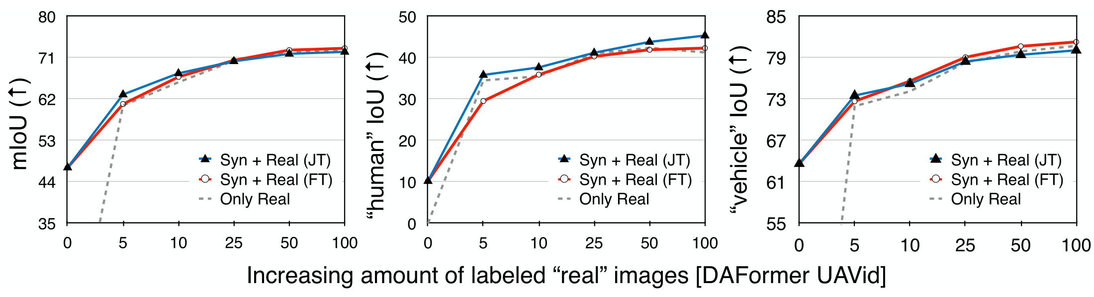
Figure 10: [DAFormer UAVid] SkyScenes can augment “real” training data. We show how SkyScenes can additionally augment real (UAVid [19]) training data. We compare DAFormer [11] models trained using only $5\%,10\%,25\%,50\%,100\%$ of labeled UAVid [19] images with counterparts that were either (1) pretrained on SkyScenes, and finetuned on UAVid [19] (FT) or (2) trained jointly on SkyScenes and UAVid [19] (JT). We find that [Left] additionally augmenting training data with SkyScenes and help improve real-world generalization in low-shot regimes, [Middle, Right] especially for under-represented classes.

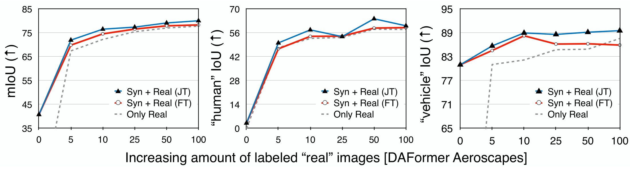
Figure 11: [DAFormer Aeroscapes] SkyScenes can augment “real” training data. We show how SkyScenes can additionally augment real (Aeroscapes [22]) training data. We compare DAFormer [11] models trained using only $5\%,10\%,25\%,50\%,100\%$ of labeled Aeroscapes [22] images with counterparts that were either (1) pretrained on SkyScenes, and finetuned on Aeroscapes [22] (FT) or (2) trained jointly on SkyScenes and Aeroscapes [22] (JT). We find that [Left] additionally augmenting training data with SkyScenes and help improve real-world generalization in low-shot regimes, [Middle, Right] especially for under-represented classes.

D.3 SkyScenes Diagnostic Experiments

Similar to Table 6 (d) in the main paper, in Table 15, we assess broader $(h,\theta)$ sensitivity of models by training DAFormer [11] models across all (total $12$) $(h,\theta)$ settings and evaluate them across the same conditions in SkyScenes. Table  15 (a) models trained on $(h=15m,\theta=0^{\circ})$ are representative of one extreme of the range (both lowest height and pitch values) – we notice that this model is extremely sensitive to height variations. From Tables 15 (a), (e) and (i), we can deduce that due to the high variability in perspective between $\theta=0^{\circ}$ and other $\theta\neq 0^{\circ}$ conditions, models trained on $\theta=0^{\circ}$ do not generalize well to other $\theta$ values. On the other hand, Tables. 15 (b), (c), (d), (f), (g) and (h) models trained on oblique perspectives are better at generalizing to other pitch conditions.

	Test mIoU ($\uparrow$)
Height	Pitch
	$\theta=0^{\circ}$	$\theta=45^{\circ}$	$\theta=60^{\circ}$	$\theta=90^{\circ}$
1 $h=15$m	72.57	66.38	57	39.46
2 $h=35$m	59.07	55.55	54.43	39.23
3 $h=60$m	48.58	44.94	43.85	31.71

(a) Height $15$ & Pitch $0^{\circ}$

	Test mIoU ($\uparrow$)
Height	Pitch
	$\theta=0^{\circ}$	$\theta=45^{\circ}$	$\theta=60^{\circ}$	$\theta=90^{\circ}$
1 $h=15$m	59.03	66.98	63.07	61.85
2 $h=35$m	43.8	49.41	49.91	45.19
3 $h=60$m	34.27	39.86	40.1	35.42

(b) Height $15$ & Pitch $45^{\circ}$

	Test mIoU ($\uparrow$)
Height	Pitch
	$\theta=0^{\circ}$	$\theta=45^{\circ}$	$\theta=60^{\circ}$	$\theta=90^{\circ}$
1 $h=15$m	45.36	64.13	68.88	69.28
2 $h=35$m	30.49	45.05	50.39	53.44
3 $h=60$m	21.86	31.21	36.51	38.43

(c) Height $15$ & Pitch $60^{\circ}$

	Test mIoU ($\uparrow$)
Height	Pitch
	$\theta=0^{\circ}$	$\theta=45^{\circ}$	$\theta=60^{\circ}$	$\theta=90^{\circ}$
1 $h=15$m	30.61	55.79	64.98	71.93
2 $h=35$m	16.84	33.2	37.89	48.63
3 $h=60$m	11.26	21.12	26.38	31.22

(d) Height $15$ & Pitch $90^{\circ}$

	Test mIoU ($\uparrow$)
Height	Pitch
	$\theta=0^{\circ}$	$\theta=45^{\circ}$	$\theta=60^{\circ}$	$\theta=90^{\circ}$
1 $h=15$m	52.14	47.62	39.04	29.31
2 $h=35$m	58.03	55.61	55.07	45.54
3 $h=60$m	53.31	50.38	50.23	46.65

(e) Height $35$ & Pitch $0^{\circ}$

	Test mIoU ($\uparrow$)
Height	Pitch
	$\theta=0^{\circ}$	$\theta=45^{\circ}$	$\theta=60^{\circ}$	$\theta=90^{\circ}$
1 $h=15$m	48.50	$50.71$	$45.22$	$42.21$
2 $h=35$m	$50.49$	$55.74$	$57.11$	$52.19$
3 $h=60$m	$45.33$	$49.79$	$50.37$	$44.62$

(f) Height $35$ & Pitch $45^{\circ}$

	Test mIoU ($\uparrow$)
Height	Pitch
	$\theta=0^{\circ}$	$\theta=45^{\circ}$	$\theta=60^{\circ}$	$\theta=90^{\circ}$
1 $h=15$m	37.21	49.04	47.42	44.93
2 $h=35$m	34.37	52.67	57.52	54.14
3 $h=60$m	29.82	44.36	48.33	44.71

(g) Height $35$ & Pitch $60^{\circ}$

	Test mIoU ($\uparrow$)
Height	Pitch
	$\theta=0^{\circ}$	$\theta=45^{\circ}$	$\theta=60^{\circ}$	$\theta=90^{\circ}$
1 $h=15$m	28.73	40.11	44.9	46
2 $h=35$m	25.89	38.98	46.26	54.02
3 $h=60$m	20.36	29.95	36.1	43.16

(h) Height $35$ & Pitch $90^{\circ}$

	Test mIoU ($\uparrow$)
Height	Pitch
	$\theta=0^{\circ}$	$\theta=45^{\circ}$	$\theta=60^{\circ}$	$\theta=90^{\circ}$
1 $h=15$m	37.59	32.89	24.53	18.35
2 $h=35$m	48.42	44.31	42.82	32.04
3 $h=60$m	51.53	48.38	47.71	39.45

(i) Height $60$ & Pitch $0^{\circ}$

	Test mIoU ($\uparrow$)
Height	Pitch
	$\theta=0^{\circ}$	$\theta=45^{\circ}$	$\theta=60^{\circ}$	$\theta=90^{\circ}$
1 $h=15$m	43.01	43.33	35.6	31.05
2 $h=35$m	52.13	57.6	58.84	51.95
3 $h=60$m	51.89	56.83	56.43	50.07

(j) Height $60$ & Pitch $45^{\circ}$

	Test mIoU ($\uparrow$)
Height	Pitch
	$\theta=0^{\circ}$	$\theta=45^{\circ}$	$\theta=60^{\circ}$	$\theta=90^{\circ}$
1 $h=15$m	38.58	43.4	36.96	32.22
2 $h=35$m	44.69	57.52	60.21	54.3
3 $h=60$m	43.24	56.68	59.27	49.18

(k) Height $60$ & Pitch $60^{\circ}$

	Test mIoU ($\uparrow$)
Height	Pitch
	$\theta=0^{\circ}$	$\theta=45^{\circ}$	$\theta=60^{\circ}$	$\theta=90^{\circ}$
1 $h=15$m	28.12	34.9	33.6	33.28
2 $h=35$m	32.76	45.32	53.71	55.27
3 $h=60$m	29.58	42.59	50.73	57.07

(l) Height $60$ & Pitch $90^{\circ}$

Table 15: Model Sensitivity to changing Height and Pitch. We evaluate a model trained on one $h,\theta$ variation (indicated by sub-table caption) across all other $h,\theta$ variations. Performant conditions are highlighted in blue.

D.4 Qualitative examples

In Fig. 12, 13 and 14, we show qualitative examples of predictions made by SkyScenes and SynDrone trained DeepLabv2 and DAFormer models on UAVid, AeroScapes, and ICG Drone respectively. In Fig. 15 and 16, we show how predictions are impacted by changing SkyScenes conditions.

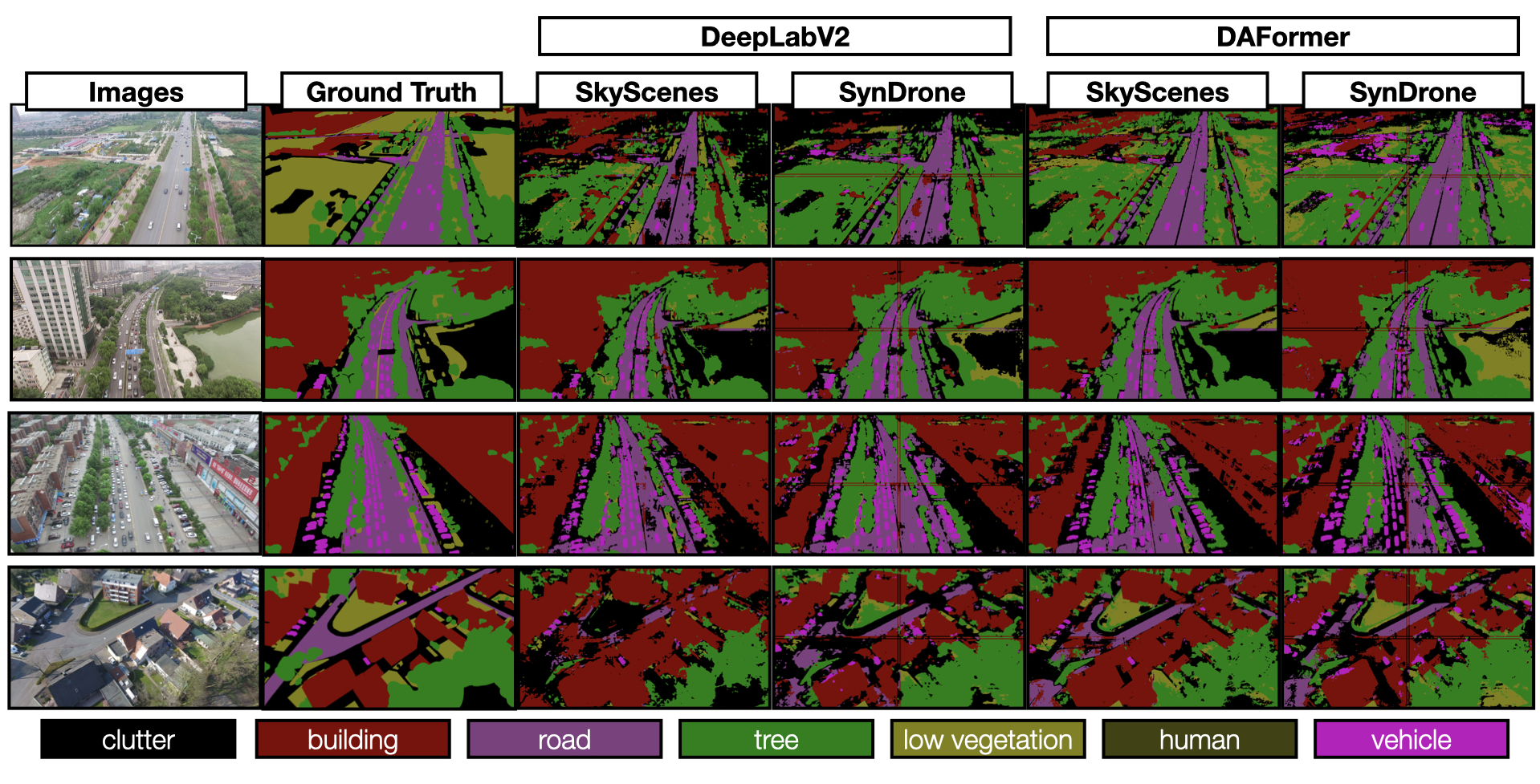
Figure 12: Synthetic $\rightarrow$UAVid Semantic Segmentation Predictions Out-of-the-box semantic segmentation predictions made on randomly selected UAVid [19] validation images by models trained on SkyScenes and SynDrone. The first two columns indicate the original image and the associated ground truth respectively, columns $3$ (SkyScenes) and $4$ (SynDrone) indicate predictions by DeepLabv2 [3] models and columns $5$ (SkyScenes) and $6$ (SynDrone) indicate predictions made by DAFormer [11] models.

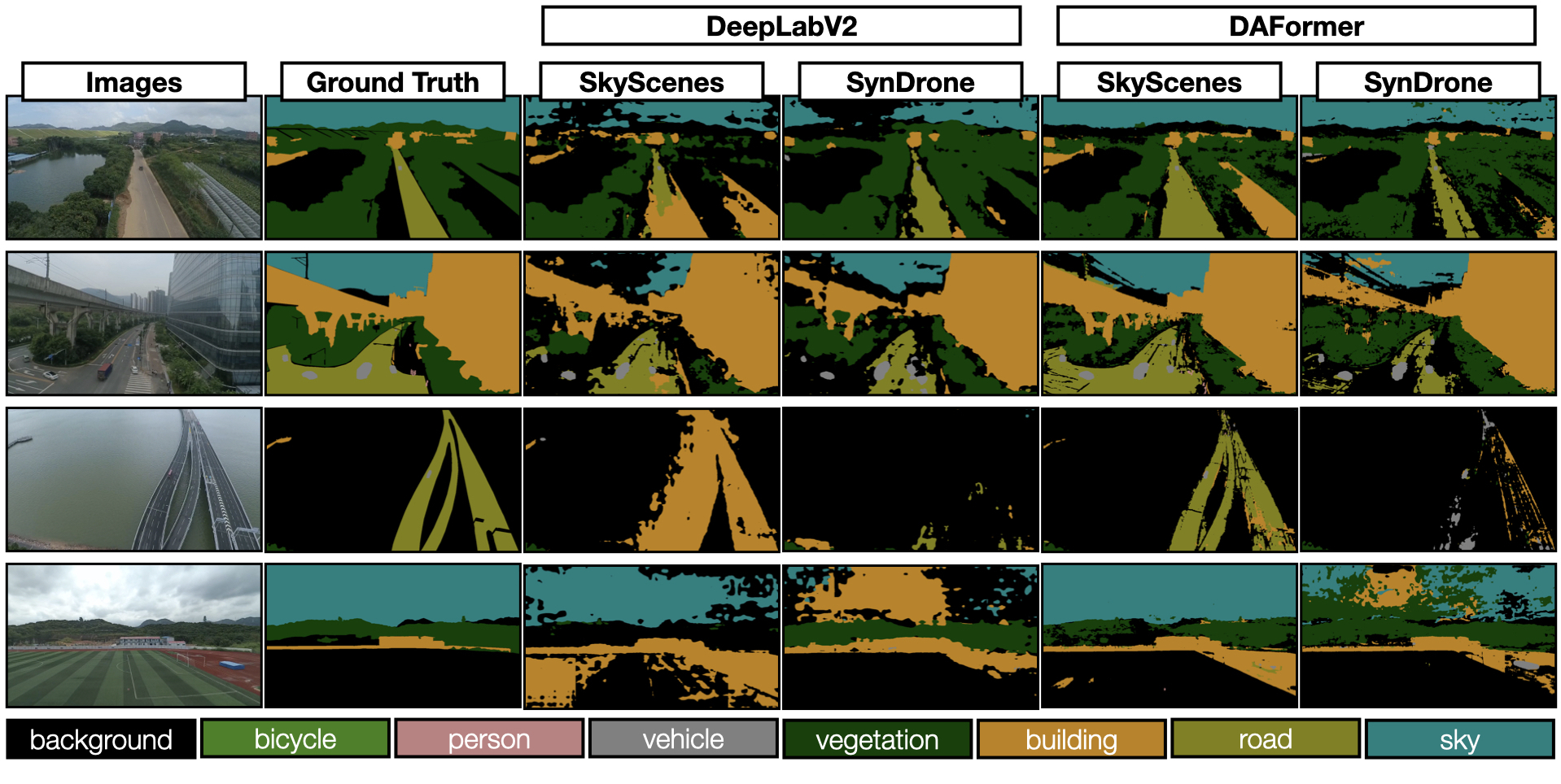
Figure 13: Synthetic $\rightarrow$AeroScapes Out of the box semantic Segmentation Predictions Out-of-the-box semantic segmentation predictions made on randomly selected AeroScapes [22] validation images by models trained on SkyScenes and SynDrone. The first two columns indicate the original image and the associated ground truth respectively, columns $3$ (SkyScenes) and $4$ (SynDrone) indicate predictions by DeepLabv2 [3] models and columns $5$ (SkyScenes) and $6$ (SynDrone) indicate predictions made by DAFormer [11] models.

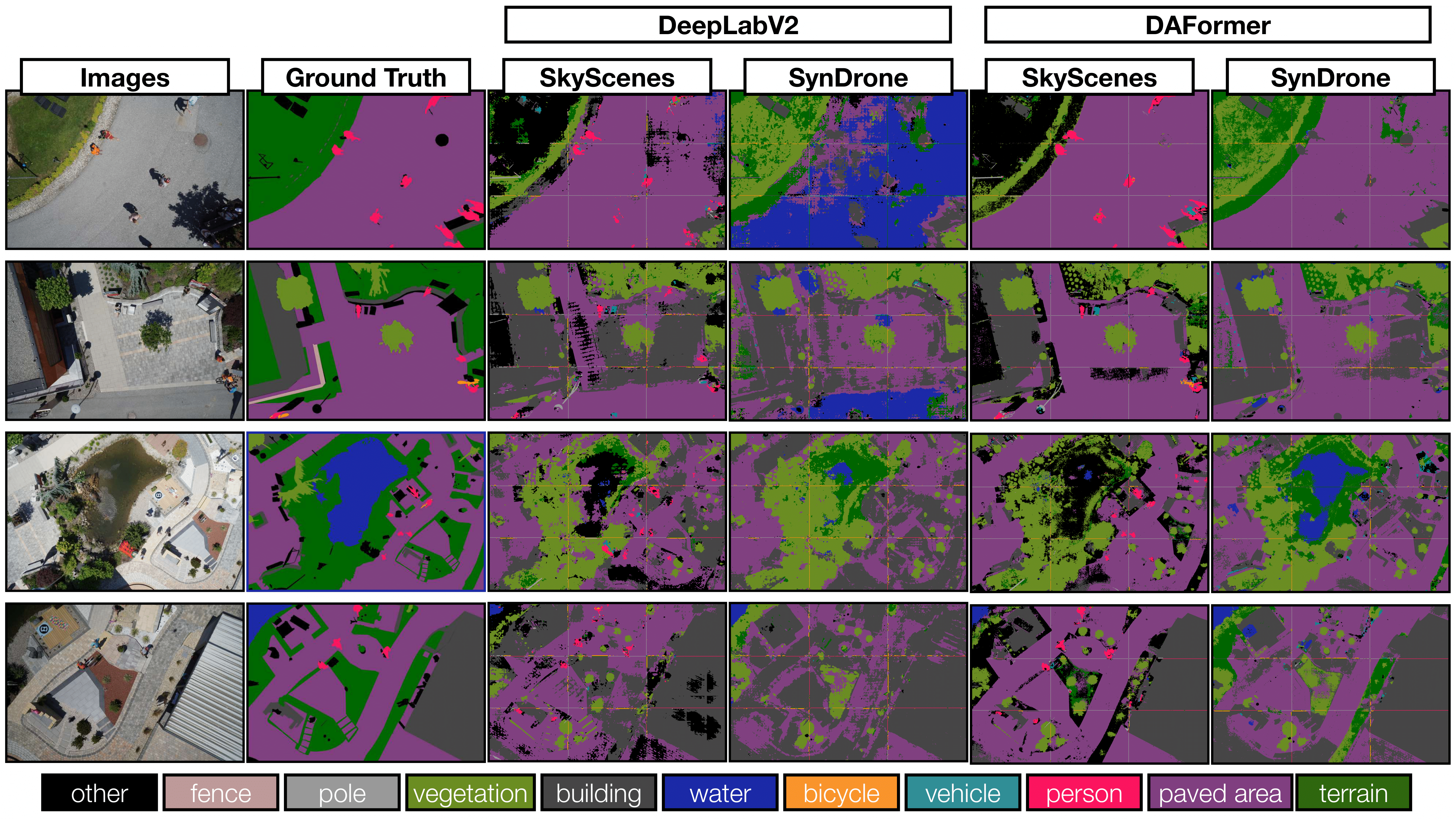
Figure 14: Synthetic $\rightarrow$ICG Drone Out of the box semantic Segmentation Predictions Out-of-the-box semantic segmentation predictions made on randomly selected ICG Drone [14] validation images by models trained on SkyScenes and SynDrone. The first two columns indicate the original image and the associated ground truth respectively, columns $3$ (SkyScenes) and $4$ (SynDrone) indicate predictions by DeepLabv2 [3] models and columns $5$ (SkyScenes) and $6$ (SynDrone) indicate predictions made by DAFormer [11] models.

Figure 15: Semantic Segmentation predictions across different daytime variations Semantic segmentation predictions made on on held-out SkyScenes images across all daytime variations by a DAFormer [11] model trained on select daytime variations. The first two columns indicate the original image and the associated ground truth, column 3 is predictions by model trained on Noon subset, column 4 is predictions by models trained on Sunset subset and column 5 is predictions by model trained on Night subset.

Figure 16: Semantic Segmentation predictions across rural and urban town variations Semantic segmentation predictions made on on held-out SkyScenes images across rural and urban scenes by a DAFormer [11] model trained on rural and urban scenes respectively. The first two columns indicate the original image and the associated ground truth, column 3 is predictions by model trained on rural scenes subset, column 4 is predictions by models trained on urban scenes subset.

References

- Cai et al. [2023] Wenxiao Cai, Ke Jin, Jinyan Hou, Cong Guo, Letian Wu, and Wankou Yang. Vdd: Varied drone dataset for semantic segmentation, 2023.
- Chen et al. [2020] Lyujie Chen, Feng Liu, Yan Zhao, Wufan Wang, Xiaming Yuan, and Jihong Zhu. Valid: A comprehensive virtual aerial image dataset. In 2020 IEEE International Conference on Robotics and Automation (ICRA), pages 2009–2016, 2020.
- Chen et al. [2017] Liang-Chieh Chen, George Papandreou, Iasonas Kokkinos, Kevin Murphy, and Alan L. Yuille. Deeplab: Semantic image segmentation with deep convolutional nets, atrous convolution, and fully connected crfs, 2017.
- Chen et al. [2018] Yu Chen, Yao Wang, Peng Lu, Yisong Chen, and Guoping Wang. Large-scale structure from motion with semantic constraints of aerial images. In Chinese Conference on Pattern Recognition and Computer Vision (PRCV), pages 347–359. Springer, 2018.
- Cordts et al. [2016] Marius Cordts, Mohamed Omran, Sebastian Ramos, Timo Rehfeld, Markus Enzweiler, Rodrigo Benenson, Uwe Franke, Stefan Roth, and Bernt Schiele. The cityscapes dataset for semantic urban scene understanding. In Proceedings of the IEEE conference on computer vision and pattern recognition, pages 3213–3223, 2016.
- Demir et al. [2018] Ilke Demir, Krzysztof Koperski, David Lindenbaum, Guan Pang, Bo Huang, Saikat Basu, Forest Hughes, Devis Tuia, Radim Raska, Abigail Kressner, et al. Deepglobe 2018: A challenge to parse the earth through satellite images. In IEEE Conference on Computer Vision and Pattern Recognition Workshops, pages 172–172, 2018.
- Dosovitskiy et al. [2017] Alexey Dosovitskiy, German Ros, Felipe Codevilla, Antonio Lopez, and Vladlen Koltun. Carla: An open urban driving simulator. In Conference on robot learning, pages 1–16. PMLR, 2017.
- Du et al. [2018] Dawei Du, Yuankai Qi, Hongyang Yu, Yifan Yang, Kaiwen Duan, Guorong Li, Weigang Zhang, Qingming Huang, and Qi Tian. The unmanned aerial vehicle benchmark: Object detection and tracking. In Proceedings of the European conference on computer vision (ECCV), pages 370–386, 2018.
- Fonder and Droogenbroeck [2019] Michael Fonder and Marc Van Droogenbroeck. Mid-air: A multi-modal dataset for extremely low altitude drone flights. In Conference on Computer Vision and Pattern Recognition Workshop (CVPRW), 2019.
- He et al. [2016] Kaiming He, Xiangyu Zhang, Shaoqing Ren, and Jian Sun. Deep residual learning for image recognition. In Proceedings of the IEEE conference on computer vision and pattern recognition, pages 770–778, 2016.
- Hoyer et al. [2022a] Lukas Hoyer, Dengxin Dai, and Luc Van Gool. Daformer: Improving network architectures and training strategies for domain-adaptive semantic segmentation, 2022a.
- Hoyer et al. [2022b] Lukas Hoyer, Dengxin Dai, and Luc Van Gool. Hrda: Context-aware high-resolution domain-adaptive semantic segmentation, 2022b.
- Hoyer et al. [2023] Lukas Hoyer, Dengxin Dai, Haoran Wang, and Luc Van Gool. Mic: Masked image consistency for context-enhanced domain adaptation, 2023.
- [14] Institute of Computer Graphics and Vision, Graz University of Technology. Semantic drone dataset. http://dronedataset.icg.tugraz.at.
- Kingma and Ba [2014] Diederik P Kingma and Jimmy Ba. Adam: A method for stochastic optimization. arXiv preprint arXiv:1412.6980, 2014.
- Lin et al. [2022] Liqiang Lin, Yilin Liu, Yue Hu, Xingguang Yan, Ke Xie, and Hui Huang. Capturing, reconstructing, and simulating: the urbanscene3d dataset. In ECCV, pages 93–109, 2022.
- Lopez-Campos and Martinez-Carranza [2021] Rafael Lopez-Campos and Jose Martinez-Carranza. Espada: Extended synthetic and photogrammetric aerial-image dataset. IEEE Robotics and Automation Letters, 6(4):7981–7988, 2021.
- Loshchilov and Hutter [2019] Ilya Loshchilov and Frank Hutter. Decoupled weight decay regularization, 2019.
- Lyu et al. [2020] Ye Lyu, George Vosselman, Gui-Song Xia, Alper Yilmaz, and Michael Ying Yang. Uavid: A semantic segmentation dataset for uav imagery. ISPRS journal of photogrammetry and remote sensing, 165:108–119, 2020.
- Maheshwari et al. [2023] Harsh Maheshwari, Yen-Cheng Liu, and Zsolt Kira. Missing modality robustness in semi-supervised multi-modal semantic segmentation, 2023.
- Neuhold et al. [2017] Gerhard Neuhold, Tobias Ollmann, Samuel Rota Bulò, and Peter Kontschieder. The mapillary vistas dataset for semantic understanding of street scenes. In 2017 IEEE International Conference on Computer Vision (ICCV), pages 5000–5009, 2017.
- Nigam et al. [2018] Ishan Nigam, Chen Huang, and Deva Ramanan. Ensemble knowledge transfer for semantic segmentation. In Proceedings of the 2018 IEEE Winter Conference on Applications of Computer Vision, pages 916–924. IEEE, 2018.
- Peng et al. [2017] Xi Peng, Bingyi Usman, Karthik Kaushik, Judy Hoffman, Dequan Wang, Kate Saenko, and Yan Zhang. Visda: The visual domain adaptation challenge. In IEEE International Conference on Computer Vision, pages 1685–1692, 2017.
- Rahnemoonfar et al. [2020] Maryam Rahnemoonfar, Tashnim Chowdhury, Argho Sarkar, Debvrat Varshney, Masoud Yari, and Robin Murphy. Floodnet: A high resolution aerial imagery dataset for post flood scene understanding, 2020.
- Rizzoli et al. [2023] Giulia Rizzoli, Francesco Barbato, Matteo Caligiuri, and Pietro Zanuttigh. Syndrone–multi-modal uav dataset for urban scenarios. arXiv preprint arXiv:2308.10491, 2023.
- Ros et al. [2016] German Ros, Laura Sellart, Joanna Materzynska, David Vazquez, and Antonio M Lopez. The synthia dataset: A large collection of synthetic images for semantic segmentation of urban scenes. In Proceedings of the IEEE conference on computer vision and pattern recognition, pages 3234–3243, 2016.
- Rottensteiner et al. [2012] Franz Rottensteiner, Gunho Sohn, Jaewook Jung, Markus Gerke, Caroline Baillard, Sébastien Bénitez, and U Breitkopf. The isprs benchmark on urban object classification and 3d building reconstruction. ISPRS Annals of Photogrammetry, Remote Sensing and Spatial Information Sciences, I-3, 2012.
- Sakaridis et al. [2019] Christos Sakaridis, Dengxin Dai, and Luc Van Gool. Guided curriculum model adaptation and uncertainty-aware evaluation for semantic nighttime image segmentation. In The IEEE International Conference on Computer Vision (ICCV), 2019.
- Sankaranarayanan et al. [2018] Swami Sankaranarayanan, Yogesh Balaji, Carlos D. Castillo, and Rama Chellappa. Generate to adapt: Aligning domains using generative adversarial networks. In The IEEE Conference on Computer Vision and Pattern Recognition (CVPR), 2018.
- Scanlon [2018] Maria Scanlon. Semantic Annotation of Aerial Images using Deep Learning, Transfer Learning, and Synthetic Training Data. PhD thesis, 2018.
- Shah et al. [2017] Shital Shah, Debadeepta Dey, Chris Lovett, and Ashish Kapoor. Airsim: High-fidelity visual and physical simulation for autonomous vehicles. In Field and Service Robotics, 2017.
- Sun et al. [2022] Tao Sun, Mattia Segu, Janis Postels, Yuxuan Wang, Luc Van Gool, Bernt Schiele, Federico Tombari, and Fisher Yu. Shift: A synthetic driving dataset for continuous multi-task domain adaptation, 2022.
- Testolina et al. [2022] Paolo Testolina, Francesco Barbato, Umberto Michieli, Marco Giordani, Pietro Zanuttigh, and Michele Zorzi. Selma: Semantic large-scale multimodal acquisitions in variable weather, daytime and viewpoints, 2022.
- Tong et al. [2020] Xin-Yi Tong, Gui-Song Xia, Qikai Lu, Huanfeng Shen, Shengyang Li, Shucheng You, and Liangpei Zhang. Land-cover classification with high-resolution remote sensing images using transferable deep models. Remote Sensing of Environment, 237:111322, 2020.
- Wang et al. [2020] Wenshan Wang, Delong Zhu, Xiangwei Wang, Yaoyu Hu, Yuheng Qiu, Chen Wang, Yafei Hu, Ashish Kapoor, and Sebastian Scherer. Tartanair: A dataset to push the limits of visual slam. 2020.
- Xie et al. [2021] Enze Xie, Wenhai Wang, Zhiding Yu, Anima Anandkumar, Jose M Alvarez, and Ping Luo. Segformer: Simple and efficient design for semantic segmentation with transformers. Advances in Neural Information Processing Systems, 34:12077–12090, 2021.
- Yu et al. [2020] Fisher Yu, Haofeng Chen, Xin Wang, Wenqi Xian, Yingying Chen, Fangchen Liu, Vashisht Madhavan, and Trevor Darrell. Bdd100k: A diverse driving dataset for heterogeneous multitask learning. In Proceedings of the IEEE/CVF conference on computer vision and pattern recognition, pages 2636–2645, 2020.
- Zhu et al. [2021] Pengfei Zhu, Longyin Wen, Dawei Du, Xiao Bian, Heng Fan, Qinghua Hu, and Haibin Ling. Detection and tracking meet drones challenge. IEEE Transactions on Pattern Analysis and Machine Intelligence, pages 1–1, 2021.