Sensitivity analysis for mixed binary quadratic programming

Abstract.

We consider sensitivity analysis for Mixed Binary Quadratic Programs (MBQPs) with respect to changing right-hand-sides (rhs). We show that even if the optimal solution of a given MBQP is known, it is NP-hard to approximate the change in objective function value with respect to changes in rhs. Next, we study algorithmic approaches to obtaining dual bounds for MBQP with changing rhs. We leverage Burer’s completely-positive (CPP) reformulation of MBQPs. Its dual is an instance of co-positive programming (COP), and can be used to obtain sensitivity bounds. We prove that strong duality between the CPP and COP problems holds if the feasible region is bounded or if the objective function is convex, while the duality gap can be strictly positive if neither condition is met. We also show that the COP dual has multiple optimal solutions, and the choice of the dual solution affects the quality of the bounds with rhs changes. We finally provide a method for finding good nearly optimal dual solutions, and we present preliminary computational results on sensitivity analysis for MBQPs.

Keywords: Sensitivity Analysis $\cdot$ Mixed Binary Quadratic Programming $\cdot$ Copositive programming $\cdot$ Duality Theory.

1. introduction

A mixed binary quadratic program (MBQP) has the form:

(1) $$z(\mathbf{b}):=\min_{\mathbf{x}\geq 0} \mathbf{x}^{\top}Q\mathbf{x}+2\mathbf{c}^{\top}\mathbf{x}$$

s.t. $$\mathbf{a}_{i}^{\top}\mathbf{x}=b_{i},\ \forall i\in\{1,\dots,m\}$$

$$x_{j}\in\{0,1\},\forall j\in\mathcal{B},$$

where $Q$ is a symmetric matrix with rational entries of size $n\times n$, $\mathbf{b}\in\mathbb{Q}^{m}$, $\mathbf{c}\in\mathbb{Q}^{n}$, $\mathbf{a}_{i}\in\mathbb{Q}^{n}$ for all $i\in\{1,\dots,m\}$, and $\mathcal{B}\subseteq\{1,\dots,n\}$ is the set of variables restricted to be binary. This is a very general optimization model that captures mixed binary linear programming [24, 10], quadratic programming [3], and several instances of mixed integer nonlinear programming models appearing in important application areas such as power systems [25].

Many practical optimization problems related to operational decision-making involve solving similar MBQP instances repeatedly. Moreover, they typically need to be solved within a short time window. This is because, unlike long-term planning problems, for such problems the exact problem data becomes available only a short time before a good solution is required to be implemented in practice. See, for examples, problems considered and discussed in [16, 19, 28]. In many of these applications, the constraint matrix remains the same, as these represent constraints related to some invariant physical resources, while the right-hand-side changes from instance to instance.

The practical consideration discussed above motivates us to study sensitivity analysis of MBQPs with respect to changing right-hand-sides. The pioneering results on sensitivity for integer programs (IPs) with changing right-hand-sides where obtained by Cook et al. [11]. See [13, 21, 12, 8] for many advances in this line of research. However, these results yield trivial bounds in the case of binary variables since they rely on the infinity norm of integer constrained variables, which is a constant for all non-zero binary vectors.

We consider an alternative approach in this paper. Specifically, we leverage Burer’s completely-positive (CPP) reformulation of MBQP [5]. The advantage of the CPP reformulation is that, although still challenging and NP-hard in general to solve, is a convex problem. Thus, one can examine its dual, which is an instance of copositive programming (COP). The optimal dual variables can provide bounds on $z(\mathbf{b})$, i.e., they allow to bound the optimal objective function of the MBQP as the right-hand-side changes. Details of the CPP reformulation and the COP dual problem are presented in the next section. This approach of using Burer’s CPP reformulation of MBQPs [5] to obtain shadow price information was first considered in [17] for the electricity market clearing problem.

Section 2 presents all our results and Section 3 provides future avenues of research. Due to lack of space, details of proofs are presented in Appendix  A and Appendix B, and some details of our experiments are presented in Appendix C.

2. Main results

Notation.

Given a positive integer $n$, we let $[n]$ denote the set $\{1,\dots,n\}$. For $u\in\mathbb{R}$, we denote its absolute value by $|u|$. For a discrete set $\mathcal{B}$, we use $|\mathcal{B}|$ to denote its cardinality. We let $\mathbb{S}^{n}$ to be the set of symmetric $n\times n$ matrices, and $\mathbb{S}^{n}_{+}$ to be the cone of $n\times n$ positive-semidefinite (PSD) matrices. We denote a matrix $M$ being PSD by $M\succeq 0$ and denote $M$ not being a PSD matrix by $M\not\succeq 0$. We let $\mathbb{S}^{n}_{p}$ be the set of symmetric $n\times n$ matrices with non-negative entries. We let $\mathcal{CP}$ to be the cone of completely positive matrices, i.e., $\mathcal{CP}=\{M\in\mathbb{S}^{n}\,|\,M=BB^{\top}\textup{ and }B\textup{ is a }m\times n\textup{ entry-wise nonnegative matrix for some integer }m\}$. We let $\mathcal{COP}$ to be the cone of copositive matrices, i.e., $\mathcal{COP}=\{M\in\mathbb{S}^{n}\,|\,\mathbf{x}^{\top}M\mathbf{x}\geq 0,\forall\mathbf{x}\geq 0\}$. We use $\mathbf{e}_{i}$ to denote the $i$-th standard basis vector.

2.1. Complexity

We begin our study by establishing formally the difficulty of approximating $z(\mathbf{b}+\Delta\mathbf{b})$ for varying $\Delta\mathbf{b}$, assuming that we know the exact value of $z(\mathbf{b})$.

Definition 2.1.

An algorithm is called $(\alpha,\beta)$-approximation for some $\beta\geq 1\geq\alpha>0$ if it takes $(A,\mathbf{b},\mathbf{c},Q,\mathcal{B},z(\mathbf{b}),\Delta\mathbf{b})$ as input, where $A$, $\mathbf{b}$, $\mathbf{c}$, $Q$, $\mathcal{B}$ represents an instance of (1), $z(\mathbf{b})$ is its optimal objective function value, $\Delta\mathbf{b}$ is the change in right-hand-side, and it outputs a scalar $p$ satisfying

$$\alpha|\Delta z|\leq p\leq\beta|\Delta z|,$$

where $\Delta z=z(\mathbf{b})-z(\mathbf{b}+\Delta\mathbf{b})$.

We note that unlike the traditional definition of approximation for optimization, the two-sided bound is necessary. Otherwise, an algorithm can “cheat” by returning either $p=0$ or $p=\infty$ depending on whether $\alpha$ or $\beta$ is not specified. For example, to achieve $p\leq\beta|\Delta z|$, the algorithm can always return $p=0$.

Our main result of this section is the following.

Theorem 2.2.

It is NP-hard to achieve $(\alpha,\beta)$-approximation for any $\beta\geq 1\geq\alpha>0$ for general MBQPs.

Our proof of Theorem 2.2 is based on a reduction from the edge chromatic number problem, using the fact that deciding whether the edge chromatic equals the max degree of a graph or one more than the max degree of a graph is NP-complete. Our proof is presented in Appendix A.

2.2. Strong duality

We first present the results from [6], which are the starting point for our analysis. Burer’s reformulation makes the following assumption:

(A) $$\mathbf{x}\geq 0,\ \mathbf{a}_{i}^{\top}\mathbf{x}=b_{i},\ \forall i\in[m]\quad\implies\quad 0\leq x_{j}\leq 1\text{ for all }j\in\mathcal{B}.$$

As mentioned in [6], if $0\leq x_{j}\leq 1$ for some $j\in\mathcal{B}$ is not implied, then we can explicitly add a constraint of the form $x_{j}+w_{j}=1$ where $w_{j}\geq 0$ is a slack variable. Thus, this assumption is without any loss of generality.

Consider the following CPP problem:

(2) $$z_{\mathcal{CP}}(\mathbf{b}):=\min \langle{C},{Y}\rangle$$

s.t. $$\langle{T},{Y}\rangle=1,$$

$$\langle{A_{i}},{Y}\rangle=2b_{i},\forall i\in[m]$$

$$\langle{AA_{i}},{Y}\rangle=b_{i}^{2},\forall i\in[m]$$

$$\langle{N_{j}},{Y}\rangle=0,\forall j\in\mathcal{B}$$

$$Y\in\mathcal{CP},$$

where $A_{i}\!=\!\begin{bmatrix}0&{\mathbf{a}}_{i}^{\!\top}\\ {\mathbf{a}}_{i}&0\end{bmatrix}$, $AA_{i}\!=\!\begin{bmatrix}0&0\\ 0&{\mathbf{a}}_{i}{\mathbf{a}}_{i}^{\!\top}\ \end{bmatrix}$, $T\!=\!\begin{bmatrix}1&0\\ 0&0\end{bmatrix}$, $N_{j}\!=\!\begin{bmatrix}0&-\mathbf{e}_{j}^{\!\top}\\ -\mathbf{e}_{j}&2\mathbf{e}_{j}\mathbf{e}_{j}^{\!\top}\end{bmatrix}$, $C\!=\!\begin{bmatrix}0&\mathbf{c}^{\!\top}\\ \mathbf{c}&Q\\ \end{bmatrix}$.

Burer [6] proves the following result.

Theorem 2.3 (Burer’s reformulation [6]).

Given a feasible MBQP in the form (1) satisfying assumption (A), then we have that $z(\mathbf{b})=z_{\mathcal{CP}}(\mathbf{b})$.

Let us now consider the dual program to (2):

(3) $$z_{\mathcal{COP}}(\mathbf{b}):=\textup{sup} -\Bigl{(}\sum\limits_{i=1}^{m}2b_{i}\alpha_{i}+b_{i}^{2}\beta_{i}\Bigr{)}-\theta$$

s.t. $$C+\sum\limits_{i=1}^{m}\Bigl{(}\alpha_{i}A_{i}+\beta_{i}AA_{i}\Bigr{)}+\Bigl{(}\sum\limits_{j\in\mathcal{B}}\gamma_{j}N_{j}\Bigr{)}+\theta T=M$$

$$M\in\mathcal{COP}.$$

Given an optimal solution to the dual (3), say $({\alpha^{*}},{\beta^{*}},{\gamma^{*}},{\theta^{*}},{M^{*}})$, and a perturbation to the right-hand-side of (1) by $\Delta b\in\mathbb{R}^{m}$, we can obtain a lower bound to $z(\mathbf{b}+\Delta b)$ as:

(4) $$z(\mathbf{b}+\Delta\mathbf{b})\geq-\Bigl{(}\sum\limits_{i=1}^{m}2(b_{i}+\Delta b_{i}){\alpha^{*}_{i}}+(b_{i}+\Delta b_{i})^{2}{\beta^{*}_{i}}\Bigr{)}-{\theta^{*}},$$

since this follows from weak duality.

If there is a positive duality gap between (2) and (3), then we do not expect the bound (4) to be strong. Understanding when strong duality holds is the topic of this section. Our results of this section are aggregated in the next theorem:

Theorem 2.4 (Strong duality).

Consider a MBQP in the form (1) satisfying the assumption (A). Let $\mathbb{P}=\{\mathbf{x}:\mathbf{a}_{i}^{\top}\mathbf{x}=b_{i},\forall i\in[m],\mathbf{x}\geq 0\}\neq\emptyset$ denote the feasible region of (1) that is assumed to be non-empty. Suppose $l$ is a finite lower bound on $z(\mathbf{b})$. Then:

1. When $\mathbb{P}$ is bounded, there is a strictly copositive feasible solution of (3) which implies strong duality holds between (2) and (3) by the Slater condition.

2. When $Q$ is PSD or $\mathbb{P}$ is bounded, there is a closed-form formula to construct a feasible solution to (3) whose objective function value is $l-\epsilon$ where $\epsilon$ can be any arbitrarily small positive number. In particular, when $l$ is the optimal value of (MBQP), this is a constructive proof that strong duality holds between (2) and (3).

3. There exists examples where $Q$ is not PSD and $\mathbb{P}$ is unbounded, such that there is a positive duality gap between (2) and (3).

4. The optimal solution of (3) is not attainable in general even if $\mathbb{P}$ is bounded and there is no duality gap.

Note that part (a) of Theorem 2.4 was shown in [4], where the authors prove that strong duality holds between (2) and (3) in a non-constructive way when $\mathbb{P}$ is bounded. Their argument utilizes a recent result from [20]. Also [22] explores similar questions in a recent presentation. To the best of our understanding, parts (b), (c), and (d) of Theorem 2.4 were not known before.

We note that in part (b) of Theorem 2.4 the promised closed form solutions can achieve additive $\epsilon$-optimal solutions for any $\epsilon>0$. Is this an artifact of our proof technique? Clearly when $Q=0$ and $\mathcal{B}=\emptyset$, the optimal solution of (3) can be achieved, as the dual optimal solution can be achieved by linear programming duality (set $\beta=0$). Part (d) shows that even if strong duality holds, the optimal solution is not attainable in (3) in general. Therefore, part (b) of Theorem 2.4 is the best we can hope for, as an optimal solution is not always achievable. Moreover, Part (d) indicates that there is no Slater point in $(\ref{CP})$ in general when $\mathbb{P}$ is bounded. One can further show via simple examples that it is possible there is no Slater point in $(\ref{COP})$ when $\mathbb{P}$ is unbounded and $Q$ is PSD.

2.2.1. Proof sketch for part (a) of Theorem 2.4:  

For the proof of this part, we show that $\hat{M}:=C+\hat{\lambda}\cdot H$ is a feasible solution of (3) and a strictly copositive matrix when $\mathbb{P}$ is bounded, where $\hat{\lambda}$ is sufficiently large positive quantity and

(5) $$H=T+\sum_{i=1}^{m}AA_{i},$$

that is, $\hat{\alpha_{i}}=0\ \forall i\in[m]$, $\hat{\beta_{i}}=\lambda\ \forall i\in[m]$, $\hat{\gamma_{j}}=0\ \forall j\in\mathcal{B}$, $\hat{\theta}=0$. Thus $\hat{M}$ is a Slater point leading to the required result. The full poof is in Section B.1.

2.2.2. Proof sketch for part (b) of Theorem 2.4:  

A key ingredient to prove this part of Theorem 2.4 is a local stability result that may be of independent interest. Consider the following perturbation of the original MBQP:

(11) $$\begin{array}[]{rl}\zeta(\mathbf{b},\epsilon):=&\min\limits_{\mathbf{x},\varepsilon^{(i)}}\mathbf{x}^{\top}Q\mathbf{x}+2\mathbf{c}^{\top}\mathbf{x}\\ &\ \ \ \ \ \mathbf{a}_{i}^{\top}\mathbf{x}=b_{i}+\varepsilon^{(1)}_{i},\forall i\in[m]\\ &\ \ \ \ \ x_{j}+\varepsilon^{(2)}_{j}\in\{0,1\},\forall j\in\mathcal{B}\\ &\ \ \ \ \ \left\lVert\varepsilon^{(r)}\right\rVert_{\infty}\leq\epsilon,\forall r\in\{1,2\}\\ &\ \ \ \ \ \mathbf{x}\geq 0.\end{array}$$

We prove the following result:

Theorem 2.5 (Local stability).

Let $l$ be a lower bound on $z(\mathbf{b})$, i.e., a lower bound on $\zeta(\mathbf{b},0)$. When $Q\text{ is PSD}$ or $\mathbb{P}$ is bounded, there exists $t_{1}>0,t_{2}\geq 0$ that depends on $A,\mathbf{b},\mathbf{c},Q,\mathcal{B}$ such that if $0\leq\epsilon<t_{1}$, then $\zeta(\mathbf{b},\epsilon)\geq l-\epsilon t_{2}$.

We note that if we were only considering the case where $Q$ is PSD, then the above result could possibly be obtained using disjunctive arguments. Since we also allow for non-PSD $Q$ matrices (when $\mathbb{P}$ is bounded), our proof of Theorem 2.5 requires the use a result from [26] characterizing the optimal solution of quadratic programs, and is presented in Appendix B.2.

The closed form solution promised in part (b) of Theorem 2.4 is built using specific building blocks or combinations of values for the variables $\alpha,\beta,\gamma,\theta$. In particular consider the following two building blocks:

(i) Building block 1.

For all $i\in[m]$, consider the following combination: $(\hat{\alpha_{i}}=-b_{i},\hat{\beta_{i}}=1,\hat{\theta}=b^{2}_{i})$ and all other variables are zero; let the resulting matrix be:

(12) $${K\!K}_{i}=\sum\limits_{i=1}^{m}\left(\hat{\alpha_{i}}A_{i}+\hat{\beta_{i}}AA_{i}\right)+\left(\sum\limits_{j\in\mathcal{B}}\hat{\gamma_{j}}N_{j}\right)+\hat{\theta}T=-b_{i}A_{i}+AA_{i}+b_{i}^{2}T.$$

Note that ${K\!K}_{i}$ is the the matrix associated to quadratic form obtained by homogenizing $(b_{i}-\mathbf{a}_{i}^{\top}\mathbf{x})^{2}$.

(ii) Building block 2.

For all $j\in\mathcal{B}$, consider the following combination: $\tilde{\alpha_{i}}=-fb_{i}\ \forall i\in[m],\tilde{\beta_{i}}=f\ \forall i\in[m],\tilde{\theta}=(f\sum_{i=1}^{m}b_{i}^{2})+r,$ and $\tilde{\gamma_{j}}=-g$; let the resulting matrix be

$$G_{j}(f,g,r) =\sum\limits_{i=1}^{m}\Bigl{(}\tilde{\alpha_{i}}A_{i}+\tilde{\beta_{i}}AA_{i}\Bigr{)}+\Bigl{(}\sum\limits_{j\in\mathcal{B}}\tilde{\gamma_{j}}N_{j}\Bigr{)}+\tilde{\theta}T$$

$$=f\Bigl{(}\sum\limits_{i=1}^{m}{K\!K}_{i}\Bigr{)}-gN_{j}+rT,$$

where $f,g,r$ are parameters.

The closed form solution that we construct for (3) is of the form:

(14) $$U(f_{1},f_{2},g,r,\tau)=C+f_{1}\Bigl{(}\sum_{i=1}^{m}{K\!K}_{i}\Bigr{)}+\sum_{j\in\mathcal{B}}G_{j}(f_{2},g,r)+\tau H-lT,$$

where $H$ is defined in (5). We specify values for the parameters $f_{1},f_{2},g,r,\tau$ such that the above matrix is copositive and has objective value of $l-\epsilon$.

Lets us first compute the objective function value of $U(f_{1},f_{2},g,r,\tau)$. Observe that for fixed values of $(f_{1},f_{2},g,r,\tau)$ we have that $\alpha_{i}=-b_{i}\cdot(f_{1}+f_{2}|\mathcal{B}|)$, $\beta_{i}=(f_{1}+f_{2}|\mathcal{B}|)+\tau$ for all $i\in[m]$ and $\theta=\sum_{i=1}^{m}b_{i}^{2}\cdot(f_{1}+f_{2}|\mathcal{B}|)+r|\mathcal{B}|+\tau-l$. Thus the objective value of $U(f_{1},f_{2},g,r,\tau)$ is

$$-\Bigl{(}\sum_{i=1}^{m}2b_{i}\alpha_{i}+b^{2}_{i}\beta_{i}\Bigr{)}-\theta=l-r\cdot|\mathcal{B}|-\tau\cdot\Bigl{(}1+\sum_{i=1}^{m}b_{i}^{2}\Bigr{)}.$$

We show that we may choose $r$ and $\tau$ to be arbitrarily small positive numbers, thus obtaining an objective value of $l-\epsilon$.

Next consider the question of showing that $U(f_{1},f_{2},g,r,\tau)$ is copositive. It is easy to verify that ${K\!K}_{i}\succeq 0$ and therefore ${K\!K}_{i}$ is copositive. We also show that for sufficiently large $f,g,r$ we have that $G_{j}(f,g,r)\in\mathcal{COP}$ and $H$ is also copositive. However, due to presence of the terms $C$ and $-lT$ in $U(f_{1},f_{2},g,r,\tau)$, one has to additionally verify its copositivity. Consider a non-negative vector $\mathbf{y}:=[t;\mathbf{x}]\geq 0$ and we need to verify that $\mathbf{y}^{\top}U(f_{1},f_{2},g,r,\tau)\mathbf{y}\geq 0$. The case when $t=0$ follows from the fact that $Q\succeq 0$ or $H$ is strictly copositive when $\mathbb{P}$ is bounded. In the case when $t>0$, the building blocks ${K\!K}_{i}$’s and $G_{j}(f,g,r)$’s behave like augmented Lagrangian penalties (see [15, 14] for strong duality results for general mixed integer convex quadratic programs) of the original constraints of the MBQP, i.e., if $\frac{1}{t}\mathbf{x}$ is not feasible for MBQP($\epsilon$) then $\mathbf{y}^{\top}U(f_{1},f_{2},g,r,\tau)\mathbf{y}$ becomes large positive value in the following fashion:

• If $|\mathbf{a}_{i}^{T}\mathbf{x}\frac{1}{t}-b_{i}|>\epsilon$, then it is easy to see that $y^{\top}{K\!K}_{i}y=|\mathbf{a}_{i}^{T}x-t\mathbf{b}_{i}|^{2}$ and this “penalty” yields that $\mathbf{y}^{\top}U(f_{1},f_{2},g,r,\tau)\mathbf{y}\geq 0$ for the selected values of parameters $(f_{1},f_{2},g,r,\tau)$.

• If $\frac{x_{j}}{t}\in(\epsilon,1-\epsilon)\cup(1+\epsilon,\infty)$ (i.e., $\frac{x_{j}}{t}$ is far from being binary), then $y^{\top}G_{j}(f,g,r)y\gg 0$ and this “penalty” yields that $\mathbf{y}^{\top}U(f_{1},f_{2},g,r,\tau)\mathbf{y}\geq 0$ for the selected values of parameters $(f_{1},f_{2},g,r,\tau)$.

• The remaining case is when $\frac{1}{t}\mathbf{x}$ is feasible for MBQP($\epsilon$). In this case it turns out that Theorem 2.5 implies that $y^{\top}U(f_{1},f_{2},g,r,\tau)y\geq 0$ for the selected values of parameters $(f_{1},f_{2},g,r,\tau)$.

The details of our proof are presented in Appendix B.3.

Finally, note that by the construction of (2), the inequality $z(\mathbf{b})\geq z_{\mathcal{CP}}(\mathbf{b})$ trivially holds. Part (b) of Theorem 2.4 shows that $z_{\mathcal{COP}}(\mathbf{b})\geq z(\mathbf{b})-\epsilon$ for any positive $\epsilon$ when $Q$ is PSD or $\mathbb{P}$ is bounded. Since $z_{\mathcal{CP}}(\mathbf{b})\geq z_{\mathcal{COP}}(\mathbf{b})$ as a consequence of weak duality, we arrive at the following observation.

Remark 2.6 (Alternative proof of Burer’s Theorem).

The proof of part (b) of Theorem 2.4 provides an alternative proof of Theorem 2.3 in the case when $Q$ is PSD or $\mathbb{P}$ is bounded.

2.2.3. Proof for part (c) of Theorem 2.4:  

We will provide an example where $Q\not\succeq 0$ and $\mathbb{P}$ is unbounded, such that (2) is feasible and has finite value while (3) is infeasible. Consider the following instance:

$$\min\{x_{1}^{2}-x_{2}^{2}|x_{1}-x_{2}=0,x_{1}\geq 0,x_{2}\geq 0\}.$$

This problem is feasible and its optimal value is zero. Hence, (2) is also feasible and has value zero by Theorem 2.3. The COP dual is:

$$\max -\theta$$

s.t $$\begin{bmatrix}0&0&0\\ 0&1&0\\ 0&0&-1\\ \end{bmatrix}+\theta\begin{bmatrix}1&0&0\\ 0&0&0\\ 0&0&0\\ \end{bmatrix}+\alpha\begin{bmatrix}0&1&-1\\ 1&0&0\\ -1&0&0\\ \end{bmatrix}+\beta\begin{bmatrix}0&0&0\\ 0&1&-1\\ 0&-1&1\\ \end{bmatrix}=:M\in\mathcal{COP}$$

We claim that the dual is infeasible. Let $\mathbf{y}=\begin{bmatrix}0\\ 1\\ 1+\epsilon\end{bmatrix}$, where $\epsilon>0$. Then

$$\mathbf{y}^{\top}M\mathbf{y} =1-(1+\epsilon)^{2}+\beta(1+(1+\epsilon)^{2}-2(1+\epsilon))=-2\epsilon+(\beta-1)\epsilon^{2}$$

When $\epsilon$ is small enough, $\mathbf{y}^{\top}M\mathbf{y}<0$. This completes the proof.

Remark 2.7 (Local stability not satisfied when $Q\not\succeq 0$ and $\mathbb{P}$ is unbounded).

It is instructive to see that the above example does not satisfy the local stability property. Indeed, for any positive value of $\epsilon$, it is straightforward to verify that $\zeta(0,\epsilon)=-\infty$, even though $\zeta(0,0)=0$. Hence, the sufficient conditions for local stability Theorem 2.5 cannot be further relaxed.

2.2.4. Part (d) of Theorem 2.4:  

The proof is in Appendix B.4.

2.3. How good is the closed form solution of Theorem 2.4 for sensitivity analysis?

Previous works consider solving (3) using cutting-plane techniques [17, 1, 2, 22] as a way to solve the original MBQP. However, in this paper we take a different perspective. We believe that with the success of modern state-of-the-art integer programming solvers, the original MBQP may be (in most cases) best solved directly using an integer programming solver. The key attraction therefore of Theorem 2.4 is to be able to build a closed-form solution (14) of the dual (3) using the optimal solution (or best known lower bound) of MBQP. One can therefore directly start conducting sensitivity analysis after solving the original MBQP and building the closed-form dual solutions.

However, conducting sensitivity analysis using dual solutions is challenging due to the presence of multiple $\epsilon$-optimal solution. First note that, given an $\epsilon$-optimal dual solution $(\alpha^{*},\beta^{*},\gamma^{*},\theta^{*})$ guaranteed by strong duality verified in Theorem 2.4, we have that $z(\mathbf{b})=-\Bigl{(}\sum\limits_{i=1}^{m}2b_{i}{\alpha^{*}_{i}}+b^{2}_{i}{\beta^{*}_{i}}\Bigr{)}-{\theta^{*}}+\epsilon.$ Subtracting the right-hand-side of the above from the right hand-side of (4), we obtain that the predicted change in the objective function value using the dual solution $(\alpha^{*},\beta^{*},\gamma^{*},\theta^{*})$ when the right-hand-side changes form $\mathbf{b}$ to $\mathbf{b}+\Delta\mathbf{b}$ is:

(15) $$\textup{Predict}(\alpha^{*},\beta^{*},\gamma^{*},\theta^{*}):=-\sum_{i=1}^{m}2\Delta b_{i}\alpha_{i}^{*}-\sum_{i=1}^{m}((\Delta b_{i})^{2}+2b_{i}\Delta b_{i})\beta_{i}^{*}-\epsilon.$$

Next consider the building block ${K\!K}_{i}$ in (12), used to construct the closed for solution in part (b) of Theorem 2.4, corresponding to $(\hat{\alpha_{i}}=-b_{i},\hat{\beta_{i}}=1,\hat{\theta}=b^{2}_{i})$. The objective function value of this block is $-(2b_{i}\hat{\alpha_{i}}+b_{i}^{2}\hat{\beta_{i}})-\hat{\theta}=0.$ Moreover, ${K\!K}_{i}\succeq 0$. Thus, we arrive at the following observation:

Proposition 2.8.

Let $\mathbf{b}^{i}\in\mathbb{R}^{m}$ be the vector with $i^{\textup{th}}$ component equal to $b_{i}$ and zeros everywhere else. If $(\alpha^{*},\beta^{*},\gamma^{*},\theta^{*},M^{*})$ is an $\epsilon$-optimal solution of (3), then $(\alpha^{*}-\mathbf{b}^{i},\beta^{*}+\mathbf{e}_{i},\gamma^{*},\theta^{*}+b_{i}^{2},M^{*}+{K\!K}_{i})$ is also an $\epsilon$-optimal solution of (3).

On the other hand, substituting $(\alpha^{*}-\mathbf{b}^{i},\beta^{*}+\mathbf{e}_{i},\gamma^{*},\theta^{*}+b_{i}^{2},M^{*}+{K\!K}_{i})$ in place of $(\alpha^{*},\beta^{*},\gamma^{*},\theta^{*},M^{*})$ in (15) we obtain:

$$\textup{Predict}(\alpha^{*}-\mathbf{b}^{i},\beta^{*}+\mathbf{e}_{i},\gamma^{*},\theta^{*}+b_{i}^{2})=\textup{Predict}(\alpha^{*},\beta^{*},\gamma^{*},\theta^{*})-(\Delta b_{i})^{2},$$

or equivalently,

$$|\textup{Predict}(\alpha^{*}-\mathbf{b}^{i},\beta^{*}+\mathbf{e}_{i},\gamma^{*},\theta^{*}+b_{i}^{2})|=|\textup{Predict}(\alpha^{*},\beta^{*},\gamma^{*},\theta^{*})|+(\Delta b_{i})^{2}.$$

Thus, we arrive at the following conclusion:

Remark 2.9.

If $(\alpha^{*},\beta^{*},\gamma^{*},\theta^{*},M^{*})$ is an $\epsilon$-optimal solutions of (3), then the lower bound obtained using the dual optimal solution $(\alpha^{*}-\mathbf{b}^{i},\beta^{*}+\mathbf{e}_{i},\gamma^{*},\theta^{*}+b_{i}^{2},M^{*}+{K\!K}_{i})$ for the right-hand-side vector $\mathbf{b}+\Delta\mathbf{b}^{i}$ is worse than that obtained by $(\alpha^{*},\beta^{*},\gamma^{*},\theta^{*},M^{*})$.

Therefore, in order to obtain the best possible sensitivity results, we would like the contribution of ${K\!K}_{i}$’s in the dual optimal matrix to be as small as possible. The main role of ${K\!K}_{i}$’s is to ensure that the constructed solution is in $\mathcal{COP}$. However, as an artifact of our proof of part (b) of Theorem 2.4, the contribution of the ${K\!K}_{i}$’s in the closed-form solution is much higher than what is really needed to ensure copositivity. This fact was empirically verified by preliminary computations.

By examining the structure of optimal solution $U(f_{1},f_{2},g,r,\tau)$ in (14) and noting that the second building block $G_{j}(f,g,r)$ is a linear combination of ${K\!K}_{i}$’s, $N_{j}$’s and $T$, we may try to find good dual solutions, with small contribution of ${K\!K}_{i}$’s and fixed values of $\tau$ and $r$, as follows:

(16) $$\min_{p,\gamma} \sum_{i=1}^{m}w_{i}p_{i}$$

s.t. $$C+\sum_{i=1}^{m}p_{i}{K\!K}_{i}+\sum_{j\in\mathcal{B}}\gamma_{j}N_{j}+\tau H-(l+r)T\in\mathcal{COP},$$

where $w_{i}$’s are some non-negative weights. Note that part (b) of Theorem 2.4 guarantees that the above problem finds an $\epsilon$ (whose value depending on $\tau$ and $r$) optimal dual solution. In our computations, we solved a variant of the above optimization problem.

2.4. Preliminary computations

2.4.1. Modifications to (16)  

The following changes are made to improve the quality of the bound and the computational cost.

Linear penalty

Consider a new building block corresponding to $\alpha_{i}=-1,\theta=2b_{i}$ and all other variables zero. This block is associated to the homogenization of the linear function $(b_{i}-\mathbf{a}_{i}^{\top}\mathbf{x})$, and it does not contribute to the objective function, just like ${K\!K}_{i}$. Setting, $K_{i}=2b_{i}T-A_{i}$, we solve the following problem:

(17) $$\min_{p,\gamma,\delta} \sum_{i=1}^{m}w_{i}^{(1)}p_{i}+w_{i}^{(2)}\delta_{i}$$

s.t. $$C+\sum_{i=1}^{m}p_{i}{K\!K}_{i}+\sum_{i=1}^{m}\delta_{i}K_{i}+\sum_{j\in\mathcal{B}}\gamma_{j}N_{j}+\tau H-(l+r)T\in\mathcal{COP},$$

Although including $K_{i}$ into the problem is not necessary, we have empirically observed that it leads to tighter sensitivity bounds due to the added degree of freedom. The heuristic choice of $\mathbf{w}^{(1)}$ and $\mathbf{w}^{(2)}$ are presented in Appendix C.

Solving a restriction of (17).

Solving a copositive program is challenging. Therefore, we replaced the restriction of being in the copositive cone in (17) with a restriction of being in the $\mathbb{S}_{+}+\mathbb{S}_{P}$. This leads to a semidefinite program, which can be solved in polynomial time. However, the resulting problem can become infeasible. To mitigate this problem, we consider two more changes:

1. Allowing non-optimal dual solutions: Instead of fixing $l$, we let $l$ become a variable. We also penalize finding a poor quality dual solution by changing the objective of (17) to: $\min_{p,\gamma,\delta,l}\ -l+\sum_{i=1}^{m}w_{i}^{(1)}p_{i}+w_{i}^{(2)}\delta_{i}.$ In this way, we may increase the chances of finding a feasible solution, However the dual solution we find may be have lesser objective than the known optimal value of original MBQP.

2. McCormick inequalities: The $Y$ variable in (2) satisfies the following well-known McCormick inequalities:

   (18) $$Y_{ij}\leq Y_{1,i},\quad Y_{ij}\leq Y_{1,j},\quad Y_{ij}\geq Y_{1,i}+Y_{1,j}-1,\quad Y_{ij}\geq 0.$$

   We add new columns to (17) corresponding to these inequalities.

2.4.2. Preliminary experimental results.

Instances.

In our preliminary experiments, we generate three classes of instances, which we refer to as (COMB), (SSLP), and (SSQP).

The first class of instances are a weighted stable set problem with a cardinality constraint:

(COMB) $$\min\bigl{\{}-\mathbf{c}^{\top}x\mid\sum_{j=1}^{n}x_{j}\leq p,\ x_{i}+x_{j}\leq 1\ \forall(i,j)\in E\bigr{\}}$$

We generate random instances in the following way. The underlying graph is a randomly generated bipartite graph $(V_{1}\cup V_{2},E)$ with $|V_{1}|=|V_{2}|=10$ and each edge $(i,j)\in E$ is present with probability $d$ where $d\in\{0.3,0.5,0.7\}$. Each entry of $c$ is uniformly sampled from $\{0,\dots,10\}$. The right-hand-side of the cardinality constraint is $p=3$. Twenty instances were generated for each choice of $d$. For this class of instances, we performed sensitivity analysis with respect to the right-hand-side of the cardinality constraint, where we increased the value of $p$ by $\Delta p\in\{1,\dots,10\}$.

The next class of instances contains continuous variables that are “turned on or off” using binary variables. The instances have the following form:

(SSLP) $$\min\ \bigl{\{}-2\mathbf{c}_{x}^{\top}\!\mathbf{x}+2\mathbf{c}_{y}^{\top}\!\mathbf{y}\mid\mathbf{a}_{i}^{\top}\!\mathbf{x}\!\leq\!b_{i}\ i\!\in\![m],\ x_{i}\!\leq\!y_{i}\ i\!\in\![n],\ x\!\geq\!0,\ y\!\in\!\{0,1\}^{n}\bigr{\}}$$

We generate instances in the following way. We set $n=20$ and $m=5$. Each entry of $\mathbf{c}_{x}$ is uniformly sampled from $\{0,\dots,10\}$ and $\mathbf{c}_{y}=(3,\dots,3)$ is a constant vector. Each entry of $\mathbf{a}_{i}$ is uniformly sampled from $\{0,\dots,10\}$ and then each entry of $\mathbf{a}_{i}$ is zeroed out with probability $d\in\{0.3,0.5,0.7\}$. Finally, $b_{i}=\lfloor\frac{1}{2}\mathbf{a}_{i}^{\top}\mathbf{e}\rfloor$ for all $i\in[m]$. Twenty instances were generated for each probability. For this class of instances, we focus on sensitivity with-respect to right-hand-side of $\mathbf{a}_{i}^{\top}x\leq b_{i},\forall i\in[m]$ when $\Delta\mathbf{b}\in\{0,1,2,3\}^{m}$.

The last class of instances is similar, except that the objective is quadratic:

(SSQP) $$\min\ \bigl{\{}-2\mathbf{c}_{x}^{\top}\!\mathbf{x}+2\mathbf{c}_{y}^{\top}\!\mathbf{y}+\mathbf{x}^{\top}\!Q\mathbf{x}\mid\mathbf{a}_{i}^{\top}\!\mathbf{x}\!\leq\!b_{i}\ i\!\in\![m],\ x_{i}\!\leq\!y_{i}\ i\!\in\![n],\ x\!\geq\!0,\ y\!\in\!\{0,1\}^{n}\bigr{\}}$$

We generate $\mathbf{c}_{x}$, $\mathbf{c}_{y}$, $\mathbf{a}_{i}$,$\mathbf{b}$ as before. The matrix $Q$ is randomly generated such that $Q=\sum\limits_{i\in\{1,2\}}\mathbf{u}_{i}\mathbf{u}_{i}^{\top}$ where each entry of $\mathbf{u}_{i}$ is uniformly sampled from $\{-1,0,1\}$.

Experiments conducted.

Our experiments are implemented in Julia 1.9, relying on Gurobi version 9.0.2 and Mosek 10.1 as the solvers. We solve on a Windows PC with 12th Gen Intel(R) Core(TM) i7 processors and 16 RAM. We compare our method with other known methods. Those methods consider certain convex relaxation of (MBQP) and obtain dual variables of constraints to conduct sensitivity analysis via weak duality. In this case, we consider three convex relaxations, which we call Shor1, Shor2, Cont.

First, we consider the the Shor relaxation of (MBQP):

$$\min_{Y\in\SS_{+}\cap\SS_{P}}\left\{\left\langle{C},{Y}\right\rangle\;\middle|\;\begin{array}[]{@{}l@{}}\left\langle{T},{Y}\right\rangle=1,\left\langle{N_{j}},{Y}\right\rangle=0,\forall j\in\mathcal{B}\\ \left\langle{A_{i}},{Y}\right\rangle=2b_{i},\forall i\in[m]\end{array}\right\}.$$

Next, we consider the relaxation of the problem obtained by augmenting Shor1 with redundant quadratic constraints and McCormick inequalities:

$$\min_{Y\in\SS_{+}\cap\SS_{P}}\left\{\left\langle{C},{Y}\right\rangle\;\middle|\;\begin{array}[]{@{}l@{}}\left\langle{T},{Y}\right\rangle=1,\left\langle{N_{j}},{Y}\right\rangle=0,\forall j\in\mathcal{B}\\ \left\langle{A_{i}},{Y}\right\rangle=2b_{i},\left\langle{AA_{i}},{Y}\right\rangle=b_{i}^{2},\forall i\in[m]\\ \text{McCormick inequalities (\ref{eq:mccormick})}\end{array}\right\}.$$

Finally, and assuming that $Q$ is PSD, we obtain a convex relaxation simply by relaxing the binary variables to be continuous variables in $[0,1]$:

$$\min_{\mathbf{x}\geq 0}\left\{\mathbf{x}^{\top}Q\mathbf{x}+2\mathbf{c}^{\top}\mathbf{x}\;\middle|\;\begin{array}[]{@{}l@{}}\mathbf{a}_{i}^{\top}\mathbf{x}=b_{i},\ \forall i\in[m],x_{j}\in[0,1]\text{ and }\forall j\in\mathcal{B}\end{array}\right\}.$$

The relaxations Shor1 and Shor2 are solved using Mosek, while the relaxation Cont is solved using Gurobi. Notice that these problems may have multiple optimal solutions, so different solvers might lead to different solutions.

We choose relaxation Shor1 as a baseline and measure the goodness of those predictions by relative gap. Given rhs change $\Delta\mathbf{b}$, ground-truth $z(\mathbf{b}+\Delta\mathbf{b})$, the prediction $p_{1}$ by Shor1 and the prediction $p_{2}$ by some method, then

$$\text{relative gap}=\frac{z(\mathbf{b}+\Delta\mathbf{b})-p_{2}}{z(\mathbf{b}+\Delta\mathbf{b})-p_{1}}.$$

This is always a non-negative number and the smaller relative gap the better performance of the given method.

Results and discussion

Figure 1 shows an example of bounds obtained using different methods. Tables 1, 3, and 3 summarize the relative gaps obtained in the experiments mentioned above. Appendix C provides a more detailed information, including relative gaps per density.

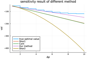
(a) a (COMB) instance with $d=0.3$

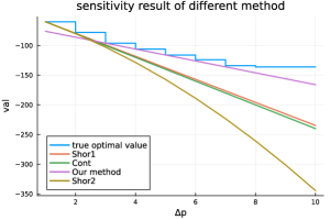
(b) a (COMB) instance with $d=0.5$

Figure 1. Two randomly generated (COMB) instances with $d=0.3$ and $d=0.5$. The x-axis corresponds to $\Delta p$ and y-axis corresponds to optimal value of the new program or different predicted value of different methods.

‘ $\Delta k$ 1 2 3 4 5 6 7 8 9 10 avg time(s) Shor1 1 1 1 1 1 1 1 1 1 1 7.30 Shor2 1.33 2.04 2.7 2.71 2.76 2.79 2.87 2.88 2.94 3.03 10.17 our method 0.83 0.02 0.00 0.11 0.19 0.26 0.32 0.38 0.41 0.44 8.35 Cont 0.97 1.07 1.09 1.08 1.07 1.06 1.05 1.05 1.04 1.04 0.00

Table 1. Average relative gap (COMB) – all densities

Table 2. Average relative gap for (SSLP) – all densities

$\left\lVert\Delta\mathbf{b}\right\rVert_{\infty}$	$\leq 1$	$\leq 2$	$\leq 3$	avg time(s)
Shor1	1	1	1	3.63
Shor2	1.20	1.48	1.64	7.21
our method	0.59	0.55	0.60	5.82
Cont	1.00	1.00	1.00	0.00

Table 3. Average relative gap for (SSQP) – all densities

$\left\lVert\Delta\mathbf{b}\right\rVert_{\infty}$	$\leq 1$	$\leq 2$	$\leq 3$	avg time(s)
Shor1	1	1	1	3.58
Shor2	1.24	1.39	1.54	7.08
our method	0.52	0.48	0.53	5.90
Cont	1.00	1.00	1.00	0.00

We observe that our method provides the tightest sensitivity bounds in all cases. Also note that method Shor2 provides the worst bounds. This is easier to observe in Figure 1. This is interesting, because the SDP from Shor2 is quite similar to Burer’s formulation (with additional McCormick inequalities). This discrepancy is most likely due to the fact that these problems have multiple optimal solutions - similar to the discussion in Section 2.3. The naive Shor2 approach finds an optimal dual which does not give good bounds after $\mathbf{b}$ is perturbed. On the other hand, our method attempts to find a good dual solution (with respect to producing good bounds for changing rhs) inside the $\epsilon$-optimal face of the dual.

3. Conclusion and future direction

We proved sufficient conditions for strong duality to hold between Burer’s reformulation of MBQPs and its dual. One direction of research is to extend such strong duality results for reformulations of more general QCQPs [7].

We have proposed a SDP-based algorithm to conduct sensitivity analysis of general (MBQP) which provides much better bounds than existing methods. This algorithm is motivated by the structure of $\epsilon$-optimal solution of the COP dual. However, the sizes of instances we can currently perform sensitivity analysis are limited by the SDP solver. One possible future direction is to develop a more scalable solver for the SDP in (17), for instance, using the techniques from [23].

Appendix A Hardness of approximation

In this section we prove Theorem 2.2, which states that the sensitivity problem for (MBQP) is NP-hard to approximate. Specifically, we show that computing an $(\alpha,\beta)$-approximation is NP-hard even if all variables are binary. Our strategy is to create a trivial binary integer linear program which after changing one entry of $\mathbf{b}$ by one captures a hard combinatorial property. The hard combinatorial property we use are edge colorings of graphs.

Let $G=(V,E)$ be a simple graph. An edge coloring of $G$ is an assignment of colors to edges so that no incident edge will have the same color. The minimum number of colors required is called edge chromatic number and denoted by $\chi^{\prime}(G)$. The classical theory by Vizing [27] states that:

Theorem A.1 (Vizing theorem).

For any simple graph $G$, $\chi^{\prime}(G)\in\{\Delta(G),\Delta(G)+1\}$ where $\Delta(G)$ is the maximum degree of vertices in $G$.

Although Vizing theorem restricts edge chromatic number to two choices, it is still hard to distinguish between these two choices. In fact, edge chromatic number is hard even in the special case of cubic graphs, which are simple graph with every vertex having degree three.

Theorem A.2 ([18]).

It is NP-hard to determine the edge chromatic number of cubic graphs.

We can express edge coloring as an MBQP problem. Given a graph $G=(V,E)$ and an upper bound $H$ of its edge chromatic number $\chi^{\prime}(G)$, then the classic formulation is

$$\min\sum_{i\in[H]}w_{i}$$

$$\text{s.t. }\sum_{i\in[H]}x_{ei}=1,\forall e\in E$$

$$\ \ \ \ \ x_{ri}+x_{si}\leq w_{i},\forall r,s\in E,r\cap s\neq\emptyset,\forall i\in[H]$$

$$\ \ \ \ \ x\in\{0,1\}^{|E|\times[H]},w\in\{0,1\}^{[H]}$$

Here $w_{i}=1$ means $i^{th}$ color is used and $x_{ri}=1$ means edge $r$ is colored to be $i$. The first set of constraints requires that every edge must be colored by exactly one color. The second set of constraints requires that no adjacent edge will receive the same color.

When the given graph $G$ is a cubic graph, then $H=4$ is an upper bound on $\chi^{\prime}(G)$ by Vizing Theorem. Consider the following program:

$$z_{1}:=\min\sum_{i\in[H]}w_{i}$$

$$\text{s.t. }\sum_{i\in[H]}-w_{i}\leq-4$$

$$\ \ \ \ \ \sum_{i\in[H]}x_{ei}=1,\forall e\in E$$

$$\ \ \ \ \ x_{ri}+x_{si}\leq w_{i},\forall r,s\in E,r\cap s\neq\emptyset,\forall i\in[H]$$

$$\ \ \ \ \ x\in\{0,1\}^{|E|\times[H]},w\in\{0,1\}^{[H]}$$

By Vizing Theorem, the optimal value $z_{1}$ is $4$. When we change the first constraint from $\sum_{i\in[H]}-w_{i}\leq-4$ to $\sum_{i\in[H]}-w_{i}\leq-3$, we obtain the following program:

$$z_{2}:=\min\sum_{i\in[H]}w_{i}$$

$$\text{s.t. }\sum_{i\in[H]}-w_{i}\leq-3$$

$$\ \ \ \ \ \sum_{i\in[H]}x_{ei}=1,\forall e\in E$$

$$\ \ \ \ \ x_{ri}+x_{si}\leq w_{i},\forall r,s\in E,r\cap s\neq\emptyset,\forall i\in[H]$$

$$\ \ \ \ \ x\in\{0,1\}^{|E|\times[H]},w\in\{0,1\}^{[H]}$$

of Theorem 2.2.

Let $z_{1},z_{2}$ be the same as above. If the graph is $3$-edge-colorable, then $z_{2}=3$ and $|\Delta z|=1$. Otherwise, $z_{2}=4$ and $|\Delta z|=0$. In this case, any $(\alpha,\beta)$-approximation with $\beta\geq\alpha>0$ will return $p>0$ if and only if the graph is $3$-edge-colorable. This implies that any such $(\alpha,\beta)$-approximation is NP-hard. ∎

Appendix B Duality theorem

In this section we prove Theorem 2.4, which characterizes when strong duality holds between (2) and (3). Assume that the lower bound of the optimal value (MBQP) is known in advance and denote by $l$. Recall that the feasible region (MBQP) is

$$\mathbb{P}=\{\mathbf{x}:\mathbf{a}_{i}^{\top}\mathbf{x}=b_{i},\forall i\in[m],\mathbf{x}\geq 0\}\neq\emptyset.$$

In remaining part of this paper, we will introduce many new constants and functions. We present the following table to where those constants and functions are defined.

Table 4. notation table

name	source
$k$	Lemma B.1
$t_{0}$	Lemma B.10
$t_{1}$	Theorem 2.5
$t_{2}$	Theorem 2.5
$t_{3}$	Proposition B.3
$h(\cdot)$	Remark B.5
$\mu(\cdot)$	Remark B.6
$\eta$	Theorem B.12
$\rho$	Theorem B.12

This section is organized into several subsections. Each of the parts of Theorem 2.4 is proved in a separate subsection. There is another subsection for the proof of Theorem 2.5, which is used in the proof of Part (b) of Theorem 2.4.

B.1. Theorem 2.4(a): Slater point when $\mathbb{P}$ is bounded

Lemma B.1.

Let $H:=T+\sum\limits_{i\in[m]}AA_{i}$. When $\mathbb{P}$ is bounded, then $H$ is strictly copositive. Therefore, there exists some number $k>0$ that depends on $A$ such that $H-kI\in\mathcal{COP}$.

Proof.

$H$ is a sum of PSD matrix and therefore $H$ is clearly copositive. We prove that $H$ is strictly copositive by showing that for every non-zero $\mathbf{y}:=[t;\mathbf{x}]\geq 0$, $\mathbf{y}^{\top}H\mathbf{y}>0$. When $t>0$, this is clearly true since $\mathbf{y}^{\top}H\mathbf{y}\geq\mathbf{y}^{\top}T\mathbf{y}=t>0$. Thus, we may consider the case when $t=0$. Suppose $H$ is not strictly copositive, then there exists some $\mathbf{y}^{\prime}:=[0;\mathbf{x}^{\prime}]\geq 0$ ($\mathbf{x}^{\prime}\neq 0$) such that $(\mathbf{y}^{\prime})^{\top}H\mathbf{y}^{\prime}=0$. This implies that

$$(\mathbf{y}^{\prime})^{\top}AA_{i}\mathbf{y}^{\prime}=(\mathbf{a}_{i}^{\top}\mathbf{x}^{\prime})^{2}=0,\forall i\in[m]\implies\mathbf{a}_{i}^{\top}\mathbf{x}^{\prime}=0,\forall i\in[m].$$

Note that since by assumption the constraints $\mathbf{x}\in\mathbb{P}$ imply that $0\leq x_{j}\leq 1$ for all $j\in\mathcal{B}$, we have that $\mathbf{a}_{i}^{\top}\mathbf{x}^{\prime}=0,\forall i\in[m]$ implies $x_{j}^{\prime}=0,\forall j\in\mathcal{B}$. Thus, $\mathbf{x}^{\prime}$ is a non-zero recession direction of $\mathbb{P}$, implying that $\mathbb{P}$ is unbounded which leads to contradiction. ∎

of Part (a) of Theorem 2.4.

By Lemma B.1, $H$ is strictly copositive and therefore $C+\lambda H$ is strictly copositive for some sufficiently large $\lambda>0$. By Slater condition, strong duality holds between (2) and (3). ∎

B.2. Theorem 2.5: Local stability

For a fixed $\mathbf{b}$, we will refer the feasible region of (MBQP($\epsilon$)) by $\mathcal{S}(\epsilon)$. $\mathcal{S}(\epsilon)$ is defined by some linear constraints and set of constraints $x_{j}+\varepsilon^{(2)}_{j}\in\{0,1\},\forall j\in\mathcal{B}$. Since there are only finitely many choice of $x_{j}+\varepsilon^{(2)}_{j}$, $\mathcal{S}(\epsilon)$ can be viewed as a union of finitely many polyhedrons. For any $\mathbf{w}\in\{0,1\}^{\mathcal{B}}$, we define

$$\mathcal{S}(\epsilon,\mathbf{w}):=\left\{(\mathbf{x}\ \varepsilon^{(i)})\;\middle|\;\begin{array}[]{@{}l@{}}\mathbf{a}_{i}^{\top}\mathbf{x}=b_{i}+\varepsilon^{(1)}_{i},\forall i\in[m]\\ x_{j}+\varepsilon^{(2)}_{j}=w_{j},\forall j\in\mathcal{B}\\ \left\lVert\varepsilon^{(r)}\right\rVert_{\infty}\leq\epsilon,\forall r\in\{1,2\}\\ \mathbf{x}\geq 0\end{array}\right\}.$$

$$\zeta(\mathbf{b},\epsilon,\mathbf{w}):=\min_{\mathbf{x},\varepsilon^{(i)}}\{\mathbf{x}^{\top}Q\mathbf{x}+2\mathbf{c}^{\top}\mathbf{x}:(\mathbf{x}\ \varepsilon^{(i)})\in\mathcal{S}(\epsilon,\mathbf{w})\}.$$

$$N(\epsilon):=\{\mathbf{w}\in\{0,1\}^{\mathcal{B}}:\mathcal{S}(\epsilon,\mathbf{w})\neq\emptyset\}.$$

$$\hbox{\vbox{\hrule height=0.5pt\kern 2.15277pt\hbox{\kern-1.00006pt$N(\epsilon)$\kern-1.00006pt}}}:=\{0,1\}^{\mathcal{B}}\setminus N(\epsilon).$$

Under this definition, we have

$$\mathcal{S}(\epsilon)=\bigcup\limits_{\mathbf{w}\in\{0,1\}^{\mathcal{B}}}\mathcal{S}(\epsilon,\mathbf{w})=\bigcup\limits_{\mathbf{w}\in N(\epsilon)}\mathcal{S}(\epsilon,\mathbf{w}).$$

$$\zeta(\mathbf{b},\epsilon)=\min\limits_{\mathbf{w}\in\{0,1\}^{\mathcal{B}}}\zeta(\mathbf{b},\epsilon,\mathbf{w})=\min\limits_{\mathbf{w}\in N(\epsilon)}\zeta(\mathbf{b},\epsilon,\mathbf{w}).$$

We will prove that when $Q$ is PSD (including $Q=0$) or $\mathbb{P}$ is bounded, $\zeta(\mathbf{b},\epsilon)$ can be lower bounded by some linear function on $\epsilon$ if $\mathbf{b}$ is fixed and $\epsilon$ is small.

To prove Theorem 2.5, we will establish several other statements. Our main idea is to reduce obtaining lower bound on $\zeta(\mathbf{b},\epsilon)$ to finding the lower bound of finitely many quadratic programming problems. In particularly, we will use Vavasis’s result on characterization of optimal solution of general quadratic programming in [26] and show that the lower bound on $\zeta(\mathbf{b},\epsilon)$ can be viewed as piece-wise quadratic function on $\epsilon$ when $\epsilon$ is sufficiently small.

Proposition B.2.

For any fixed $\epsilon\geq 0$, if $\mathbb{P}$ is bounded, then $\mathcal{S}(\epsilon)$ is bounded. Moreover, $\mathcal{S}(\epsilon_{1})\subseteq\mathcal{S}(\epsilon_{2})$ for all $\epsilon_{2}\geq\epsilon_{1}\geq 0$.

Proof.

For any $\epsilon_{1}\leq\epsilon_{2}$, if $[\mathbf{x};\varepsilon^{(i)}]\in\mathcal{S}({\epsilon_{1}})$, then clearly $[\mathbf{x};\varepsilon^{(i)}]\in\mathcal{S}({\epsilon_{2}})$. This proves $\mathcal{S}(\epsilon_{1})\subseteq\mathcal{S}(\epsilon_{2})$. To see that boundedness of $\mathbb{P}$ implies boundedness of $\mathcal{S}({\epsilon})$, we prove the contrapositive statement, i.e., if $\mathcal{S}({\epsilon})$ is unbounded, then $\mathbb{P}$ is unbounded. Suppose $\mathcal{S}({\epsilon})$ is unbounded, then consider its standard relaxation

$$\mathcal{S}^{\text{relax}}(\epsilon):=\left\{(\mathbf{x}\ \varepsilon^{(i)})\;\middle|\;\begin{array}[]{@{}l@{}}\mathbf{a}_{i}^{\top}\mathbf{x}=b_{i}+\varepsilon^{(1)}_{i},\forall i\in[m]\\ x_{j}+\varepsilon^{(2)}_{j}\in[0,1],\forall j\in\mathcal{B}\\ \left\lVert\varepsilon^{(r)}\right\rVert_{\infty}\leq\epsilon,\forall r\in\{1,2\}\\ \mathbf{x}\geq 0\end{array}\right\}.$$

Since $\mathcal{S}^{\text{relax}}(\epsilon)$ is the relaxation of $\mathcal{S}(\epsilon)$, $\mathcal{S}^{\text{relax}}(\epsilon)$ is also unbounded. Note $\mathcal{S}^{\text{relax}}(\epsilon)$ is defined by some linear constraints, this means there exists non-zero $[\mathbf{x}_{0};\varepsilon^{(i)}_{0}]$ such that $\mathbf{a}_{i}^{\top}\mathbf{x}_{0}=(\varepsilon^{(1)}_{0})_{i},\forall i\in[m],(\mathbf{x}_{0})_{j}+(\varepsilon^{(2)}_{0})_{j}=0,\forall j\in\mathcal{B},(\varepsilon^{(r)}_{0})_{t}=0,\forall r\in\{1,2\},\mathbf{x}_{0}\geq 0$. Rewriting those conditions, it yields there exists some non-zero $[\mathbf{x}_{0}]$ such that $\mathbf{a}_{i}^{\top}\mathbf{x}_{0}=0,\forall i\in[m],(\mathbf{x}_{0})_{j}=0,\forall j\in\mathcal{B},\mathbf{x}_{0}\geq 0$. This implies that $\mathbb{P}$ is unbounded. ∎

Proposition B.3.

There exists some threshold $t_{3}>0$ that only depends on $A,\mathbf{b},\mathcal{B}$ such that if $0\leq\epsilon<t_{3}$, then $N(\epsilon)=N(0)$.

Proof.

Observe that $\mathcal{S}(0,\mathbf{w})\subseteq\mathcal{S}(\epsilon,\mathbf{w})$ for all $\mathbf{w}\in\{0,1\}^{\mathcal{B}}$. This implies $N(0)\subseteq N(\epsilon)$. It suffices to show when $\epsilon$ is sufficiently small, for all $\mathbf{w}\in\hbox{\vbox{\hrule height=0.5pt\kern 2.15277pt\hbox{\kern-1.00006pt$N(0)$\kern-1.00006pt}}}$, we have that $\mathbf{w}\in\hbox{\vbox{\hrule height=0.5pt\kern 2.15277pt\hbox{\kern-1.00006pt$N(\epsilon)$\kern-1.00006pt}}}$. For any $\mathbf{w}\in\hbox{\vbox{\hrule height=0.5pt\kern 2.15277pt\hbox{\kern-1.00006pt$N(0)$\kern-1.00006pt}}}$, consider the following linear programming:

(23) $$\begin{array}[]{rl}t_{\mathbf{w}}:=&\min\varphi\\ &\text{s.t. }b_{i}-\varphi\leq\mathbf{a}_{i}^{\top}\mathbf{x}\leq b_{i}+\varphi,\forall i\in[m]\\ &\ \ \ \ \ x_{j}=w_{j},\forall j\in\mathcal{B}\\ &\ \ \ \ \ \mathbf{x}\geq 0,\varphi\geq 0.\end{array}$$

This linear program is clearly feasible by choosing $\varphi$ to be sufficiently large. Moreover, $t_{\mathbf{w}}>0$. Otherwise, this will imply that $\mathbf{w}\in N(0)$. Since this linear program is bounded from below and feasible, its optimal $t_{\mathbf{w}}$ exists and $t_{\mathbf{w}}>0$ ($t_{\mathbf{w}}$ can not arbitrarily go to $0$ due to the attainability of linear programming). If $\epsilon>0$ is sufficiently small such that

$$\max_{i\in[m]}(1+\left\lVert\mathbf{a}_{i}\right\rVert_{1})\epsilon<t_{\mathbf{w}},$$

then we claim that $\mathbf{w}\in\overline{N(0)}$ implies  $N(\epsilon)$ . Suppose not, $\mathbf{w}\in N(\epsilon)$ and then $S(\epsilon,\mathbf{w})\neq\emptyset$. That is, there exists some $\bar{\mathbf{x}},\bar{\varepsilon}^{(i)}$ such that

$$\mathbf{a}_{i}^{\top}\bar{\mathbf{x}}+\bar{\varepsilon}^{(1)}_{i}=b_{i},\forall i\in[m]$$

$$\bar{x}_{j}+\bar{\varepsilon}^{(2)}_{j}=w_{j},\forall j\in\mathcal{B}$$

$$\left\lVert\bar{\varepsilon}^{(r)}\right\rVert_{\infty}\leq\epsilon,r\in\{1,2\}$$

$$\bar{\mathbf{x}}\geq 0$$

Then we can construct a feasible solution $\mathbf{x}^{*}$ for (23) where $x^{*}_{j}:=\begin{cases}\bar{x}_{j}&\text{ if }j\notin\mathcal{B}\\ \bar{x}_{j}+\bar{\varepsilon}_{j}^{(2)}&\text{ if }j\in\mathcal{B}.\end{cases}$. In this case, for any $i\in[m]$, it follows

$$|\mathbf{a}_{i}^{\top}\mathbf{x}^{*}-b_{i}| =|\mathbf{a}_{i}^{\top}\bar{\mathbf{x}}+(\sum_{j\in\mathcal{B}}\bar{\varepsilon}_{j}^{(2)}(\mathbf{a}_{i})_{j})-b_{i}|$$

$$=|-\bar{\varepsilon}^{(1)}_{i}+\sum_{j\in\mathcal{B}}\bar{\varepsilon}_{j}^{(2)}(\mathbf{a}_{i})_{j}|$$

$$\leq(1+\left\lVert\mathbf{a}_{i}\right\rVert_{1})\epsilon$$

$$<t_{\mathbf{w}}.$$

This contradicts the fact that $t_{\mathbf{w}}$ is the optimal value of (23).

Therefore to ensure $N(\epsilon)=N(0)$ , one can choose $t_{3}:=\frac{\min\limits_{\mathbf{w}\in\overline{N(0)}}t_{\mathbf{w}}}{\max\limits_{i\in[m]}(1+\left\lVert\mathbf{a}_{i}\right\rVert_{1})}>0$. ∎

Proposition B.4.

When $Q$ is PSD or $\mathbb{P}$ is bounded, then $\zeta(\mathbf{b},\epsilon,\mathbf{w})$ exists for all $\epsilon\geq 0$ and $\mathbf{w}\in N(\epsilon)$.

Proof.

If $\mathbb{P}$ is bounded, then $\mathcal{S}(\epsilon)$ is bounded by Proposition B.2. Since $\mathcal{S}(\epsilon,\mathbf{w})\subseteq\mathcal{S}(\epsilon)$, we have that $\mathcal{S}(\epsilon,\mathbf{w})$ is bounded as well. Thus $\zeta(\mathbf{b},\epsilon,\mathbf{w})$ is the optimal value of minimizing a quadratic over a compact set and therefore $\zeta(\mathbf{b},\epsilon,\mathbf{w})$ exists.

If $Q$ is PSD, we will use Vavasis’ characterization of optimal solution of quadratic programming in [26]. We would like to point out when $Q=0$, there is a simpler argument. When $Q=0$, $\zeta(\mathbf{b},\epsilon,\mathbf{w})$ is the optimal value of some linear program whose right-hand-side is parameterized by $\epsilon$. When $\epsilon=0$, $\zeta(\mathbf{b},0,\mathbf{w})$ exists and therefore this linear program is both dual feasible and primal feasible. When $\epsilon>0$, the corresponding linear program is primal feasible as $\mathcal{S}(0,\mathbf{w})\subseteq\mathcal{S}(\epsilon,\mathbf{w})$. Moreover, the feasible region of the dual linear program remains the same and therefore it is dual feasible. In this case, $\zeta(\mathbf{b},\epsilon,\mathbf{w})$ exists.

When $Q\neq 0$ and $Q$ is PSD, suppose $\zeta(\mathbf{b},\epsilon,\mathbf{w})$ does not exist. By the result of [26],$\zeta(\mathbf{b},\epsilon,\mathbf{w})$ must diverge to negative infinity and there exists $\bar{\mathbf{x}}$, $\bar{\varepsilon}^{(1)}$, $\bar{\varepsilon}^{(2)},\mathbf{d}_{0},\mathbf{d}_{1},\mathbf{d}_{2}$ such that for all large enough $t$, $[\bar{\mathbf{x}}+t\mathbf{d}_{0};\bar{\varepsilon}^{(1)}+t\mathbf{d}_{1};\bar{\varepsilon}^{(2)}+t\mathbf{d}_{2}]$ is feasible and has a decreasing objective function. Since $\mathcal{S}(\epsilon,\mathbf{w})$ is defined by some linear constraints, this implies that $\mathbf{d}_{1}=0,\mathbf{d}_{2}=0,\mathbf{a}_{i}^{\top}\mathbf{d}_{0}=0,\forall i\in[m]\text{ and }(\mathbf{d}_{0})_{j}=0,\forall j\in\mathcal{B}\text{ and }\mathbf{d}_{0}\geq 0$. Its objective function takes form of $(\bar{\mathbf{x}}+t\mathbf{d}_{0})^{\top}Q(\bar{\mathbf{x}}+t\mathbf{d}_{0})+2\mathbf{c}^{\top}(\bar{\mathbf{x}}+t\mathbf{d}_{0})=(\bar{\mathbf{x}})^{\top}Q\bar{\mathbf{x}}+2t\mathbf{d}_{0}^{\top}Q\bar{\mathbf{x}}+t^{2}\mathbf{d}_{0}^{\top}Q\mathbf{d}_{0}+2\mathbf{c}^{\top}\bar{\mathbf{x}}+2t\mathbf{c}^{\top}\mathbf{d}_{0}$. Since for all large $t$, the objective function is decreasing with large enough $t$ and $Q$ is PSD, it must be that $\mathbf{d}_{0}^{\top}Q\mathbf{d}_{0}=0$ and therefore $Q\mathbf{d}_{0}=0$, since $Q$ is PSD. This further implies that $\mathbf{c}^{\top}\mathbf{d}_{0}<0$ since the objective function is decreasing. In this case, there exists some $\mathbf{d}_{0}$ such that $Q\mathbf{d}_{0}=0$ and $\mathbf{c}^{\top}\mathbf{d}_{0}<0$ and $\mathbf{a}_{i}^{\top}\mathbf{d}_{0}=0,\forall i\in[m]\text{ and }(\mathbf{d}_{0})_{j}=0,\forall j\in\mathcal{B}\text{ and }\mathbf{d}_{0}\geq 0$. Pick any $\mathbf{x}\in\mathcal{S}(0,\mathbf{w})$, one can verify that $\mathbf{x}+t\mathbf{d}_{0}$ is feasible for all $t\geq 0$ and its objective value goes to negative infinity as $t$ goes to infinity. This shows the $\zeta(\mathbf{b},0,\mathbf{w})$ diverges to negative infinity, which leads to a contradiction.

∎

Now we are ready to present a proof for Theorem 2.5.

of Theorem 2.5.

By Proposition B.3, when $\epsilon<t_{3}$ for some $t_{3}>0$ only depends on $A,\mathbf{b},\mathcal{B}$ , $N(\epsilon)=N(0)$. Pick any $\mathbf{w}\in N(\epsilon)$, we would like to study $\zeta(\mathbf{b},\epsilon,\mathbf{w})$ which is the value function of a quadratic program whose right-hand side is parameterized by $\epsilon$. By Proposition B.4, $\zeta(\mathbf{b},\epsilon,\mathbf{w})$ is finite. Now we are going to use Vavasis characterization of optimal solution of quadratic program in [26]. Consider any quadratic program (possibly non-convex) of form

$$\text{qv}(\mathbf{g}):= \min\mathbf{y}^{\top}H\mathbf{y}+2\mathbf{d}^{\top}\mathbf{y}$$

$$\textbf{s.t. }M\mathbf{y}\leq\mathbf{g}.$$

Vavasis [26] proved that any quadratic program with finite optimal value can be reduced to a certain convex quadratic program $Q_{\tilde{M}}:$

(26) $$\begin{array}[]{rl}&\min_{\mathbf{y}}\mathbf{y}^{\top}H\mathbf{y}+2\mathbf{d}^{\top}\mathbf{y}\\ &\text{s.t. }\tilde{M}\mathbf{y}=\tilde{\mathbf{g}},\end{array}$$

where (i) $\tilde{M}$ is a $(k+l)\times n$ matrix and first $k$ rows corresponding to some $k$ inequalities of original inequalities $M\mathbf{y}\leq\mathbf{g}$ satisfied exactly and the last $l$ rows corresponding to some entries of $\mathbf{y}$ are zero and (ii) $H$ is positive definite when restricted to the special affine subspace defined by $\tilde{M}\mathbf{y}=\tilde{g}$. The key fact we need for this result is that these requirements only depends on $\tilde{M}$ and independent of $\tilde{\mathbf{g}}$. The convex program admits a unique solution $\mathbf{y}_{\tilde{M}}$ and its optimal value $\text{qv}_{\tilde{M}}(\mathbf{g})$ where $\mathbf{y}_{\tilde{M}}$ is a linear function of $\mathbf{g}$ and $\text{qv}_{\tilde{M}}(\mathbf{g})$ is a quadratic function of $\mathbf{g}$.

Note that $\mathbf{y}_{\tilde{M}}$ only satisfies some of original constraints and it is not necessarily feasible. We say $\tilde{M}$ is good if $\mathbf{y}_{\tilde{M}}$ is feasible and we say $\tilde{M}$ is almost good if $\mathbf{y}_{\tilde{M}}$ is infeasible. We denote the set of all good $\tilde{M}$ by $\mathcal{M}_{1}$ and denote the set of all almost good $\tilde{M}$ by $\mathcal{M}_{2}$. Due to the definition of $\tilde{M}$, both $\mathcal{M}_{1},\mathcal{M}_{2}$ are finite sets and $\mathcal{M}_{1}\cup\mathcal{M}_{2}$ is independent of $\mathbf{g}$. Vavasis [26] proves that optimal solution will be some $\mathbf{y}_{\tilde{M}}$ for some $\tilde{M}$ that is good.

In our case, we can express our program in inequality form to apply Vavasis’s result:

(32) $$\begin{array}[]{rl}&\min\limits_{\mathbf{x},\varepsilon^{(i)}}\mathbf{x}^{\top}Q\mathbf{x}+2\mathbf{c}^{\top}\mathbf{x}\\ &\ \ \ \ \ b_{i}-\varepsilon^{(1)}_{i}\leq\mathbf{a}_{i}^{\top}\mathbf{x}\leq b_{i}+\varepsilon^{(1)}_{i},\forall i\in[m]\\ &\ \ \ \ \ w_{j}-\varepsilon^{(2)}_{j}\leq x_{j}\leq w_{j}+\varepsilon^{(2)}_{j},\forall j\in\mathcal{B}\\ &\ \ \ \ \ 0\leq\varepsilon^{(r)}_{t}\leq\epsilon,\forall r\in\{1,2\}\\ &\ \ \ \ \ \mathbf{x}\geq 0.\end{array}$$

The right hand side depends on $\epsilon\text{ and }\mathbf{w}$. Let us we refer to $\mathcal{M}_{1},\mathcal{M}_{2},\mathbf{y}_{\tilde{M}},qv_{\tilde{M}}(\mathbf{g})$ corresponding to some $\epsilon\text{ and }\mathbf{w}$ as $\mathcal{M}_{1}(\epsilon,\mathbf{w}),\mathcal{M}_{2}(\epsilon,\mathbf{w}),\mathbf{y}(\epsilon,\mathbf{w},\tilde{M}),\text{qv}(\epsilon,\mathbf{w},\tilde{M})$. As our right hand side is a linear function of $\epsilon$, $\text{qv}(\epsilon,\mathbf{w},\tilde{M})$ is a quadratic function of $\epsilon$ once $\mathbf{w}$ and $\tilde{M}$ are fixed.

We fix some $\mathbf{w}\in N(\epsilon)$ and prove that there exists some $t_{4}>0$ depending only on $A,\mathbf{b},\mathbf{c},Q,\mathcal{B}$, such that if $\epsilon<t_{4}$, then $\mathcal{M}_{1}(\epsilon,\mathbf{w})\subseteq\mathcal{M}_{1}(0,\mathbf{w})$. As pointed out earlier $\mathcal{M}_{1}(\epsilon,\mathbf{w})\cup\mathcal{M}_{2}(\epsilon,\mathbf{w})$ is independent of right hand sides and therefore is independent of $\epsilon$. Thus it suffices to prove that $\mathcal{M}_{2}(0,\mathbf{w})\subseteq\mathcal{M}_{2}(\epsilon,\mathbf{w})$. For $\tilde{M}\in\mathcal{M}_{2}(\epsilon,\mathbf{w})$, $\mathbf{y}_{\tilde{M}}(\epsilon,\mathbf{w})$ is a continuous function of $\epsilon$ and therefore $\mathbf{a}^{\top}_{i}\mathbf{y}_{\tilde{M}}(\epsilon,\mathbf{w})$ is a continuous function of $\epsilon$. Thus, for sufficiently small values of $\epsilon$ if $\tilde{M}\in\mathcal{M}_{2}(0,\mathbf{w})$, then $\tilde{M}\in\mathcal{M}_{2}(\epsilon,\mathbf{w})$.

Thus when $\epsilon<\min\{t_{3},t_{4}\}$, we have:

$$\zeta(\mathbf{b},\epsilon) =\min_{\mathbf{w}\in N(\epsilon)}\min_{\tilde{M}\in\mathcal{M}_{1}(\epsilon,\mathbf{w})}\text{qv}(\epsilon,\mathbf{w},\tilde{M})$$

$$=\min_{\mathbf{w}\in N(0)}\min_{\tilde{M}\in\mathcal{M}_{1}(\epsilon,\mathbf{w})}\text{qv}(\epsilon,\mathbf{w},\tilde{M})$$

$$\geq\min_{\mathbf{w}\in N(0)}\min_{\tilde{M}\in\mathcal{M}_{1}(0,\mathbf{w})}\text{qv}(\epsilon,\mathbf{w},\tilde{M}):=\mathcal{T}(\epsilon).$$

$\mathcal{T}(\epsilon)$ is the lower bound of $\zeta(\mathbf{b},\epsilon)$ with $\mathcal{T}(0)=\zeta(\mathbf{b},0)\geq l$. Since there are only finitely many choice of $\mathbf{w}\text{ and }\tilde{M}$, $\mathcal{T}(\epsilon)$ is a a piece-wise quadratic function on $\epsilon$. In this case, we can lower bound $\mathcal{T}(\epsilon)$ with a linear function when $\epsilon\in[0,\min\{t_{3},t_{4}\}]$. That is, there exists some $t_{2}>0$ that depends on $A,\mathbf{b},\mathbf{c},Q,\mathcal{B}$, $\mathcal{T}(\epsilon)\geq l-t_{2}\epsilon$ for $\epsilon\in[0,\min\{t_{3},t_{4}\}]$ and this proves that $\zeta(\mathbf{b},\epsilon)\geq l-t_{2}\epsilon$ for all $\epsilon\in[0,\min\{t_{3},t_{4}\}]$. ∎

B.3. Theorem 2.4(b): Constructing near optimal solution for (COP-dual)

In this subsection we prove part (b) of Theorem 2.4 utilizing Theorem 2.5. We first consider the case where the feasible set is bounded and then the case where it is unbounded and $Q$ is PSD. Before that, we present some preliminary lemmas.

Given some number $f,g,l,\tau$, we remind the reader the two building blocks:

$${K\!K}_{i}:=b_{i}^{2}T-b_{i}A_{i}+AA_{i},\forall i\in[m],$$

$$G_{j}(f,g,r):=f\left(\sum\limits_{i\in[m]}{K\!K}_{i}\right)-gN_{j}+rT,\forall j\in\mathcal{B}.$$

and

$$H:=T+\sum_{i\in[m]}AA_{i}.$$

Also let:

$$U_{0}:=U_{0}(\tau,l):=C+\left(\sum_{i=1}^{m}\frac{|\lambda_{min}(Q)|+1}{k}{K\!K}_{i}\right)+(\tau H)+(-lT),$$

where $k$ is defined in Lemma B.1. As mentioned earlier, ${K\!K}_{i}$ will serve as a penalty block of $\mathbf{a}^{\top}_{i}\mathbf{x}=b_{i}$ and $G_{j}(f,g,r)$ will serve as a penalty block of $x_{j}\in\{0,1\}$. Consider $\mathbf{y}:=[t;\mathbf{x}]\in\mathbb{R}^{n+1}_{+}$, it follows

$$\mathbf{y}^{\top}({K\!K}_{i})\mathbf{y}^{\top}=(b_{i}t-\mathbf{a}_{i}^{\top}\mathbf{x})^{2},\forall i\in[m],$$

$$\mathbf{y}^{\top}(-N_{j})\mathbf{y}^{\top}=2x_{j}(t-x_{j}),\forall j\in\mathcal{B}.$$

Note that all of $H,{K\!K}_{i}$ are PSD matrices and therefore copositive. To see that ${K\!K}_{i}$ is PSD, note it can be written as

$${K\!K}_{i}=\begin{bmatrix}b_{i}^{2}&-b_{i}(\mathbf{a})_{i}^{\top}\\ -b_{i}\mathbf{a}_{i}&\mathbf{a}_{i}(\mathbf{a})_{i}^{\top}\end{bmatrix}=\left(\begin{bmatrix}-b_{i}\\ \mathbf{a}_{i}\end{bmatrix}\right)\left(\begin{bmatrix}-b_{i}\\ \mathbf{a}_{i}\end{bmatrix}\right)^{\top}.$$

The matrix $G_{j}(f,g,r)$ is parameterized by $f,g,r$. It is no necessarily copositive for arbitrary choice of $f,g,r$ and $G_{j}(f,g,r)$ has objective value equals to $r$. The next lemma proves that for any positive $r$ and positive $g$, one can choose sufficient large $f$ so that $G_{j}(f,g,r)$ is copositive.

In the remaining of this section, for any matrix $A\in\SS^{n+1}$, we will use $(A)_{[\mathbf{x}]}$ to refer to principal submatrix of $A$ corresponding to the indices of $[\mathbf{x}]$. We will refer other principal submatrices like $(A)_{[x_{j}]}$ in the similar manner. Recall that we make the following assumption (A):

$$\mathbf{x}\geq 0,\ \mathbf{a}_{i}^{\top}\mathbf{x}=b_{i},\ \forall i\in[m]\quad\implies\quad 0\leq x_{j}\leq 1\text{ for all }j\in\mathcal{B}.$$

We first establish several remarks related to the assumption (A).

Remark B.5.

Fix some index $j\in\mathcal{B}$ and some positive number $\eta>0$. Then for any $\mathbf{x}\geq 0\text{ such that }x_{j}\geq\eta$, there exists some strict positive number $h_{j}(\eta)>0$ that only depends on $A,b,\eta,j$ such that

$$\max\limits_{i\in[m]}|\mathbf{a}_{i}^{\top}\mathbf{x}|\geq h_{j}(\eta).$$

Proof.

Consider the following linear programming:

(37) $$\begin{array}[]{rl}h(\eta):=&\min h\\ &\text{s.t.}-h\leq\mathbf{a}^{\top}_{i}\mathbf{x}\leq h,\forall i\in[m],\\ &\ \ \ \ \ \mathbf{x}\geq 0,h\geq 0,\\ &\ \ \ \ \ x_{j}\geq\eta.\end{array}$$

(37) is clearly feasible by choosing sufficiently large $h$. Moreover, $h(\eta)>0$. Otherwise, if $h(\eta)=0$, let $\mathbf{x}^{*},h^{*}$ be the corresponding optimal solution. Note that $\mathbf{x}^{*}\neq 0$. Pick $\mathbf{x}_{0}\in\mathbb{P}$, it follows that $\mathbf{x}_{0}+\lambda\mathbf{x}^{*}\in\mathbb{P},\forall\lambda\geq 0$. With sufficiently large $\lambda$, the assumption (A) for $j\in\mathcal{B}$ will be violated. ∎

Similarly, one can prove the following remarks using the similar approach :

Remark B.6.

Fixed $j\in\mathcal{B}$ and $\eta>0$. Then for any $\mathbf{x}\geq 0\text{ such that }x_{j}\geq 1+\eta$, there exists some strict positive number $u_{j}(\eta)>0$ that only depends on $A,b,\eta,j$ such that

$$\max\limits_{i\in[m]}|\mathbf{a}_{i}^{\top}\mathbf{x}-b_{i}|\geq u_{j}(\eta).$$

Remark B.7.

For any $\mathbf{x}\geq 0$, if $\mathbf{a}_{i}^{\top}\mathbf{x}=0,\forall i\in[m]$, then $x_{j}=0,\forall i\in\mathcal{B}$.

Lemma B.8.

For any $j\in\mathcal{B},g>0,r>0$, let $h_{j}(\eta)$ be as defined in Remark B.5. There exists some strictly positive number ${p}_{j}>0$ that only depends on $A,\mathbf{b},r,g,j$ such that if $f$ satisfies

(38) $$f\geq\max\left\{\frac{2g}{h_{j}(1)^{2}},\frac{2g}{{p_{j}}^{2}},\frac{g^{2}+2rg}{r{p_{j}}^{2}}\right\},$$

then $G_{j}(f,g,r)=(f\sum\limits_{i\in[m]}{K\!K}_{i})-gN_{j}+rT$ is copositive.

Proof.

For any $\mathbf{y}=[t;\mathbf{x}]\geq 0$, we consider several cases of $\mathbf{y}$ and assert that

$$\Lambda:=\mathbf{y}^{\top}((f\sum\limits_{i\in[m]}{K\!K}_{i})-gN_{j}+rT)\mathbf{y}\geq 0.$$

Note that since both $\sum\limits_{i\in[m]}{K\!K}_{i}$ and $T$ are PSD, the only term that could potentially make $\Lambda$ negative is $-gN_{j}$.

If $t=0$, note that $(-gN_{j})_{[\mathbf{x}]}$ is a diagonal matrix with one negative entry such that $(-gN_{j})_{[x_{j}]}=-2g$ and other entries all zeros. Therefore, if $x_{j}=0$, then $\Lambda\geq 0$. If $x_{j}\neq 0$, we can further assume $x_{j}=1$ after scaling properly. Let $h_{j}(1)>0$ be the constant in Remark B.5. Then it follows that

$$\Lambda =\mathbf{y}^{\top}\left((f\sum\limits_{i\in[m]}{K\!K}_{i})-gN_{j}+rT\right)\mathbf{y}$$

$$=\mathbf{x}^{\top}\left(f\sum_{i\in[m]}\mathbf{a}_{i}\mathbf{a}_{i}^{\top}\right)\mathbf{x}-2g$$

$$=f\left(\sum_{i\in[m]}(\mathbf{a}_{i}^{\top}\mathbf{x})^{2}\right)-2g$$

$$\geq fh_{j}(1)^{2}-2g (\text{by Remark }\ref{rem_h_j})$$

$$\geq 0. (\text{by }(\ref{eq:choice_of_f_small_block}))$$

If $t\neq 0$, we may assume $t=1$ after scaling properly. If $t=1\geq x_{j}$, ${\mathbf{y}}^{\top}(-gN_{j}){\mathbf{y}}^{\top}\geq 0$. Since all ${K\!K}_{i}$ and $T$ are PSD, then $\Lambda\geq 0.$ Thus it remains to consider the case when $t<x_{j},t=1$ and let $v:=x_{j}-t=x_{j}-1>0$. If $v\leq\min\{\frac{r}{4g},1\}$, then it follows that

$$\Lambda =\mathbf{y}^{\top}\left((f\sum\limits_{i\in[m]}{K\!K}_{i})-gN_{j}+rT\right)\mathbf{y}$$

$$\geq\mathbf{y}^{\top}\left(-gN_{j}+rT\right)\mathbf{y}$$

$$=-2g(v+1)v+r$$

$$\geq-4gv+r (0\leq v\leq 1)$$

$$\geq 0. (v\leq\frac{r}{4g})$$

So we may assume that $v\geq\min\{\frac{r}{4g},1\}$. In this case, we show that at least one of $|\mathbf{a}^{\top}\mathbf{x}_{i}-b_{i}|$ is considerably large and increases at least linearly with respect to $v$. To be more precise, we are considering the following linear fractional programming:

(44) $$\begin{array}[]{rl}p_{j}:=&\min\limits_{\mathbf{x},\psi,v}\frac{\psi}{v}\\ &\text{s.t. }b_{i}-\psi\leq\mathbf{a}_{i}^{\top}\mathbf{x}\leq b_{i}+\psi,\forall i\in[m],\\ &\ \ \ \ \ x_{j}\geq 1+v,\\ &\ \ \ \ \ v\geq\min\{\frac{r}{4g},1\},\\ &\ \ \ \ \ \mathbf{x}\geq 0,\psi\geq 0.\end{array}$$

This linear fractional programming can be exactly formulated as the following linear programming, which is known as Charnes-Cooper transformation [9].

(50) $$\begin{array}[]{rl}{p_{j}}:=&\min\limits_{\tilde{\mathbf{x}},\tilde{\psi},\tilde{v},s}\tilde{\psi}\\ &\text{s.t. }b_{i}s-\tilde{\psi}\leq\mathbf{a}_{i}^{\top}\tilde{\mathbf{x}}\leq b_{i}s+\tilde{\psi},\forall i\in[m],\\ &\ \ \ \ \ \tilde{\mathbf{x}}_{j}\geq s+\tilde{v},\\ &\ \ \ \ \ \tilde{v}\geq\min\{\frac{r}{4g},1\}s,\\ &\ \ \ \ \ \tilde{\mathbf{x}}\geq 0,s\geq 0,\tilde{\psi}\geq 0,\tilde{v}=1.\end{array}$$

We can further claim that ${p_{j}}>0$ otherwise if ${p_{j}}=0$ and let $\tilde{\mathbf{x}^{*}},\tilde{\psi^{*}},\tilde{v^{*}},s^{*}$ be the corresponding optimal solution of (50). If $s^{*}=0$, then $\mathbf{a}_{i}^{\top}\tilde{\mathbf{x}^{*}}=0,\forall i\in[m]$. By Remark B.7, this implies that $\tilde{\mathbf{x}_{j}}=0$. However, this contradicts that $\tilde{\mathbf{x}}_{j}\geq s+\tilde{v}\geq 1$. In the case when $s^{*}>0$, one can again verify that $\frac{\tilde{\mathbf{x}^{*}}}{s^{*}}$ will violate assumption (A) by using Remark B.6. Finally, it follows that

$$\Lambda =\mathbf{y}^{\top}\left(\left(f\sum\limits_{i\in[m]}{K\!K}_{i}\right)-gN_{j}+rT\right)\mathbf{y}$$

$$=f\left(\sum_{i\in[m]}(\mathbf{a}_{i}^{\top}\mathbf{x}-b_{i})^{2}\right)-2g(v+1)v+r$$

$$\geq f{p_{j}}^{2}v^{2}-2g(v+1)v+r (\text{by the definition of }{p_{j}})$$

$$=(f{p_{j}}^{2}-2g)v^{2}-2gv+r$$

$$\geq 0. (\text{by }(\ref{eq:choice_of_f_small_block}))$$

The last inequality comes from the fact that the lower bound $(f{p_{j}}^{2}-2g)v^{2}-2gv+r)$ is a quadratic function with respect to $v$. If $f{p_{j}}^{2}-2g\geq 0$ and $g^{2}-r(f{p_{j}}^{2}-2g)\leq 0$, then this lower bound is non-negative for all $v$ and this condition is guaranteed by our choice of $f$. ∎

Remark B.9.

Consider two symmetric matrices $A,B$ such that $B\underset{\mathcal{COP}}{\succeq}\eta I$ for some $\eta>0$, then $A+\frac{|\lambda_{min}(A)|+1}{\eta}B$ is strictly copositive.

Lemma B.10.

Recall $U_{0}=U_{0}(\tau,l)=C+\left(\sum_{i=1}^{m}\frac{|\lambda_{min}(Q)|+1}{k}{K\!K}_{i}\right)+(\tau H)+(-lT)$. If $\mathbb{P}$ is bounded, then there exists some $t_{0}>0$ that only depends on $A,\mathbf{b},\mathbf{c},Q,l,\tau$ such that for any $\mathbf{y}:=[t\ \mathbf{x}]\geq 0$ with $t<t_{0}$ and $\left\lVert[t\ \mathbf{x}]\right\rVert_{2}=1$, $\mathbf{y}^{\top}U_{0}\mathbf{y}\geq 0$.

Proof.

We first show that $(U_{0})_{[\mathbf{x}]}$ is strictly copositive. By Lemma B.1, we have $H\underset{\mathcal{COP}}{\succeq}kI$. This implies that $(H)_{[\mathbf{x}]}\underset{\mathcal{COP}}{\succeq}kI$. As $(H)_{[\mathbf{x}]}=\sum\limits_{i\in[m]}\mathbf{a}_{i}(\mathbf{a}_{i})^{\top}$, this means that $\sum\limits_{i\in[m]}\mathbf{a}_{i}(\mathbf{a}_{i})^{\top}\underset{\mathcal{COP}}{\succeq}kI$. Applying Remark B.9, we obtain that $(U_{0})_{[\mathbf{x}]}=Q+\frac{|\lambda_{min}(Q)|+1}{k}(\sum\limits_{i\in[m]}(\mathbf{a}_{i}\mathbf{a}_{i}^{\top}))+\tau H_{[x]}$ is strictly copositive. Consider the following program:

$$t_{0}:= \min t$$

$$\text{s.t. }\mathbf{y}=[t\ \mathbf{x}]\geq 0,$$

$$\ \ \ \ \ \left\lVert\mathbf{y}\right\rVert_{2}=1,$$

$$\ \ \ \ \ \mathbf{y}^{\top}U_{0}\mathbf{y}\leq 0.$$

If this program is infeasible, we may set $t_{0}=\infty$. Since the feasible region is a compact set and if this program is feasible, the optimal value exists and is attained. We first claim that $t_{0}>0$. Otherwise, there exits some $\mathbf{y}^{\prime}:=[0;\mathbf{x}^{\prime}]\geq 0$ such that $(\mathbf{y}^{\prime})^{\top}U_{0}\mathbf{y}^{\prime}\leq 0$. This contradicts the fact that $(U_{0})_{[\mathbf{x}]}$ is strictly copositive. In this case, the definition of $t_{0}$ guarantees that for any $\mathbf{y}:=[t;\mathbf{x}]\geq 0$ with $t<t_{0}$ and $\left\lVert[t\ \mathbf{x}]\right\rVert_{2}=1$, $\mathbf{y}^{\top}U_{0}\mathbf{y}>0$. ∎

We proceed to prove Part (b) of Theorem 2.4 in the case that the feasible set is bounded.

Theorem B.11.

(Part (b) of Theorem 2.4- bounded case) Let $l$ be the lower bound of the optimal value of (MBQP) that is $l\leq z(\mathbf{b})$ and $l_{+}:=\max\{l,0\}$. Let $k$ be the constant defined in Lemma B.1, let $t_{1},t_{2}$ be as in Theorem 2.5 and let $u_{j}(\cdot)$ be the constant defined in Remark B.6. When $\mathbb{P}$ is bounded, for any $\epsilon_{0}\in(0,t_{1})$ and any $r>0$,

$$U:=U(f_{1},f_{2},g,r,\tau,l):=C+f_{1}\left(\sum_{i\in[m]}{K\!K}_{i}\right)+\sum_{j\in\mathcal{B}}G_{j}(f_{2},g,r)+\tau H-lT$$

is copositive for $f_{1},f_{2},g,\alpha$ satisfying the following rules:

1. $f_{2},g,r$ satisfies the condition in Lemma B.8 so that $G_{j}(f_{2},g,r)$ is copositive,

2. $\tau=\frac{\epsilon_{0}t_{2}}{k}$,

3. $t_{0}$ is defined in Lemma B.10, which depends on $\tau,l$ and therefore depends on $\epsilon_{0},l$,

4. $f_{1}\geq\max\left\{\frac{|\lambda_{min}(Q)|+1}{k},\frac{-\lambda_{\min}(C)+l_{+}}{t_{0}^{2}\epsilon^{2}_{0}},\max\limits_{j\in\mathcal{B}}\{\frac{\lambda_{\min}(C)+l_{+}}{t_{0}^{2}u_{j}(\epsilon_{0})^{2}}\}\right\}$,

5. $g\geq\frac{\lambda_{\min}(C)-l_{+}}{2\epsilon^{2}_{0}t_{0}^{2}}$.

Moreover, the objective value of $U$ is $l-\tau\cdot(1+\sum\limits_{i\in[m]}b_{i}^{2})-r\cdot|\mathcal{B}|$. This objective value can be arbitrarily closed to $l$ as $r$ and $\epsilon_{0}$ goes to zero.

We would like to point out our bound in Theorem B.11 is rather loose and we are only seeking sufficient condition to ensure $U$ is copositive. We begin to prove Theorem B.11.

Proof.

By (rule.iv), it follows that

$$f_{1}-\frac{|\lambda_{min}(Q)|+1}{k}\geq 0.$$

This further implies

$$U-U_{0}=\left(f_{1}-\frac{|\lambda_{min}(Q)|+1}{k}\right)\left(\sum_{i\in[m]}{K\!K}_{i}\right)+\sum_{j\in\mathcal{B}}G_{j}(f_{2},g,r)\underset{\mathcal{COP}}{\succeq}0.$$

Combining with Lemma B.10, this implies that there exists some $t_{0}>0$ such that any $\mathbf{y}:=[t\ \mathbf{x}]\geq 0$ with $t<t_{0}$ and $\left\lVert[t\ \mathbf{x}]\right\rVert_{2}=1$, $\mathbf{y}^{\top}U\mathbf{y}\geq 0$. Thus we can assume that $t\geq t_{0}$ and define the following two sets:

(51) $$\mathrm{I}(\epsilon_{0}):=\left\{(t,\mathbf{x})\geq 0:\frac{x_{j}}{t}\in[0,\epsilon_{0}]\cup[1-\epsilon_{0},1+\epsilon_{0}],\forall j\in\mathcal{B}\right\},$$

(52) $$\mathbb{P}(\epsilon_{0}):=\left\{(t,\mathbf{x})\geq 0:\frac{1}{t}(\mathbf{a}_{i}^{\top}\mathbf{x})\in[b_{i}-\epsilon_{0},b_{i}+\epsilon_{0}],\forall i\in[m]\right\}.$$

One interpretation of such sets is that $\mathrm{I}(\epsilon_{0})$ is the approximate version of $0$-$1$ integrality and $\mathbb{P}(\epsilon_{0})$ is the approximate version of $\mathbb{P}$.

Now assume $\mathbf{y}\geq 0:=[t;\mathbf{x}]$ with $\left\lVert\mathbf{y}\right\rVert_{2}=1$ and $t\geq t_{0}$. We are going to prove that for all such $\mathbf{y}\geq 0,\mathbf{y}^{\top}U\mathbf{y}\geq 0$. We consider three cases:

1. $[t\ \mathbf{x}]\in\hbox{\vbox{\hrule height=0.5pt\kern 2.15277pt\hbox{\kern-1.00006pt$\mathbb{P}(\epsilon_{0})$\kern-1.00006pt}}}$

2. $[t\ \mathbf{x}]\in\mathbb{P}(\epsilon_{0})\cap\mathrm{I}(\epsilon_{0})$

3. $[t\ \mathbf{x}]\in\mathbb{P}(\epsilon_{0})\cap\hbox{\vbox{\hrule height=0.5pt\kern 2.15277pt\hbox{\kern-1.00006pt$\mathrm{I}(\epsilon_{0})$\kern-1.00006pt}}}$

Recall that

$$\mathbf{y}^{\top}U\mathbf{y} =\mathbf{y}^{\top}C\mathbf{y}+\sum_{i\in[m]}\underbrace{\mathbf{y}^{\top}f_{1}({K\!K}_{i})\mathbf{y}}_{\geq 0}+\sum_{j\in\mathcal{B}}\underbrace{\mathbf{y}^{\top}(G_{j}(f_{2},g,r))\mathbf{y}}_{\geq 0}+\underbrace{\mathbf{y}^{\top}\tau H\mathbf{y}}_{\geq 0}-\mathbf{y}^{\top}lT\mathbf{y}$$

The only term that only potentially makes $\mathbf{y}^{\top}U\mathbf{y}$ negative is $\mathbf{y}^{\top}C\mathbf{y}+\mathbf{y}^{\top}(-lT)\mathbf{y}$. Given $\left\lVert\mathbf{y}\right\rVert_{2}=1$, a (trivial) lower bound on $\mathbf{y}^{\top}C\mathbf{y}+\mathbf{y}^{\top}(-lT)\mathbf{y}$ is

(53) $$\mathbf{y}^{\top}C\mathbf{y}+\mathbf{y}^{\top}(-lT)\mathbf{y} =\mathbf{y}^{\top}C\mathbf{y}-t^{2}l\geq\lambda_{\min}(C)-l_{+}.$$

(case.1) If $[t;\mathbf{x}]\in\hbox{\vbox{\hrule height=0.5pt\kern 2.15277pt\hbox{\kern-1.00006pt$\mathbb{P}(\epsilon_{0})$\kern-1.00006pt}}}$, there must exist an index $e\in[m]$ such that

(54) $$\left|\frac{1}{t}(\mathbf{a}_{e}^{\top}\mathbf{x})-b_{e}\right|>\epsilon_{0}.$$

It follows that

$$\mathbf{y}^{\top}U\mathbf{y} \geq\mathbf{y}^{\top}C\mathbf{y}+\mathbf{y}^{\top}(-lT)\mathbf{y}+\mathbf{y}^{\top}{K\!K}_{i}\mathbf{y}$$

$$=\mathbf{y}^{\top}C\mathbf{y}+\mathbf{y}^{\top}(-lT)\mathbf{y}+t^{2}f_{1}\left(\frac{1}{t}(\mathbf{a}_{e}^{\top}\mathbf{x}+s_{e})-b_{e}\right)^{2}$$

$$\geq\lambda_{\min}(C)-l_{+}+t_{0}^{2}f_{1}\epsilon^{2}_{0}\ (\text{by }(\ref{trivial_lower_bound}),(\ref{eq:case1_bounded}))$$

$$\geq 0 (\text{by }\ref{rule:4}).$$

(case.2) If $[t;\mathbf{x}]\in\mathbb{P}(\epsilon_{0})\cap\mathrm{I}(\epsilon_{0})$, then $\frac{1}{t}(\mathbf{x})$ is a feasible solution of MBIP($\epsilon_{0}$). Since $\epsilon_{0}<t_{1}$ by our choice, Theorem 2.5 implies that

(55) $$\left(\frac{1}{t}\mathbf{x}\right)^{\top}Q\left(\frac{1}{t}\mathbf{x}\right)+2\mathbf{c}^{\top}\frac{1}{t}\mathbf{x}\geq l-t_{2}\epsilon_{0}.$$

Therefore, it follows that

$$\mathbf{y}^{\top}U\mathbf{y} \geq\mathbf{y}^{\top}C\mathbf{y}+\mathbf{y}^{\top}(-lT)\mathbf{y}+\mathbf{y}^{\top}\tau H\mathbf{y}$$

$$=\mathbf{x}^{\top}Q\mathbf{x}+2t\mathbf{c}\mathbf{x}+t^{2}(-l)+\mathbf{y}^{\top}\tau H\mathbf{y}$$

$$=t^{2}\left(\left(\frac{1}{t}\mathbf{x}\right)^{\top}Q\left(\frac{1}{t}\mathbf{x}\right)+2\mathbf{c}^{\top}\frac{1}{t}\mathbf{x}-l\right)+\mathbf{y}^{\top}\tau H\mathbf{y}$$

$$\geq t^{2}(l-t_{2}\epsilon_{0}-l)+\mathbf{y}^{\top}\tau H\mathbf{y} (\text{by }(\ref{eq:case2_bounded}))$$

$$\geq(-t_{2}\epsilon_{0})+\tau k (H\text{ is strictly copositive and }t\leq 1)$$

$$=0 (\text{by }\ref{rule:3}).$$

(case.3) If $[t;\mathbf{x}]\in\mathbb{P}(\epsilon_{0})\cap\hbox{\vbox{\hrule height=0.5pt\kern 2.15277pt\hbox{\kern-1.00006pt$\mathrm{I}(\epsilon_{0})$\kern-1.00006pt}}}$, this implies that there exists $e\in\mathcal{B}$ such that

$$\text{either }\frac{x_{e}}{t}\in(1+\epsilon_{0},\infty)\text{ or }\frac{x_{e}}{t}\in(\epsilon_{0},1-\epsilon_{0}).$$

If $\frac{x_{e}}{t}\in(1+\epsilon_{0},\infty)$, by Remark B.6, there exists some $w\in[m]$, some $e\in\mathcal{B}$ and some $u_{e}(\epsilon_{0})>0$ such that

(56) $$\left|\frac{1}{t}(\mathbf{a}_{w}^{\top}\mathbf{x})-b_{w}\right|>u_{e}(\epsilon_{0})$$

and it follows that

$$\mathbf{y}^{\top}U\mathbf{y} \geq\mathbf{y}^{\top}C\mathbf{y}+\mathbf{y}^{\top}(-lT)\mathbf{y}+\mathbf{y}^{\top}{K\!K}_{w}\mathbf{y}$$

$$=\mathbf{y}^{\top}C\mathbf{y}+\mathbf{y}^{\top}(-lT)\mathbf{y}+t^{2}f_{1}\left(\frac{1}{t}(\mathbf{a}_{w}^{\top}\mathbf{x})-b_{w}\right)^{2}$$

$$\geq\lambda_{\min}(C)-l_{+}+t_{0}^{2}f_{1}{u_{e}(\epsilon_{0})}^{2}\ (\text{by }(\ref{trivial_lower_bound}),(\ref{eq:case3_bounded}))$$

$$\geq 0 (\text{by }\ref{rule:4}).$$

If $\frac{x_{e}}{t}\in(\epsilon_{0},1-\epsilon_{0})$, this implies that

(57) $$x_{e}\geq\epsilon_{0}t\geq\epsilon_{0}t_{0}\text{ and }t-x_{e}\geq\epsilon_{0}t\geq\epsilon_{0}t_{0}.$$

Therefore, it follows that

$$\mathbf{y}^{\top}U\mathbf{y} \geq\mathbf{y}^{\top}C\mathbf{y}+\mathbf{y}^{\top}(-lT)\mathbf{y}+\mathbf{y}^{\top}(G_{e}(f_{2},g,r))\mathbf{y}$$

$$\geq\lambda_{\min}(C)-l_{+}+\mathbf{y}^{\top}(G_{e}(f_{2},g,r))\mathbf{y} (\text{by }(\ref{trivial_lower_bound}))$$

$$\geq\lambda_{\min}(C)-l_{+}+\mathbf{y}^{\top}(-gN_{j})\mathbf{y}$$

$$=\lambda_{\min}(C)-l_{+}+2g(t-x_{e})x_{e}$$

$$\geq\lambda_{\min}(C)-l_{+}+2g\epsilon^{2}_{0}t_{0}^{2} (\text{by }\ref{eq:case3_bounded_last})$$

$$\geq 0 (\text{by }\ref{rule:5}).$$

This completes the proof. ∎

We now consider the case where the feasible set is unbounded and $Q$ is PSD. The construction is similar to the one in Theorem B.11, but the argument is slightly more complex since Lemmas B.1 and B.10 fail in the unbounded case. Instead, we will make use of Theorem 2.5 and Lemma B.8, which hold when $Q$ is PSD. We will also use that $Q$ can be written as $VV^{\top}$ for some $V$.

Theorem B.12.

(Part (b) of Theorem 2.4 - unbounded case) Let $l$ be the lower bound of the optimal value that $l\leq z(\mathbf{b})$. Let $t_{1},t_{2}$ be the same in Theorem 2.5 and let $u_{j}(\cdot)$ the same in Remark B.6. When $Q$ is PSD, there exists some $\rho,\tau>0$ that only depend on $A,\mathbf{b},\mathbf{c},Q,\mathcal{B}$, such that for any $\epsilon_{0}\in(0,t_{1})$ and any $r>0$,

$$U:=U(f_{1},f_{2},g,r,\alpha,l)=C+f_{1}\left(\sum\limits_{i\in[m]}{K\!K}_{i}\right)+\sum\limits_{j\in\mathcal{B}}G_{j}(f_{2},g,r)+\tau H-lT$$

is copositive for $f_{1},f_{2},g,\tau$ satisfying the following rules:

1. $f_{2},g,r$ satisfies the condition in Lemma B.8 so that $G_{j}(f_{2},g,r)$ is copositive,

2. $\tau=t_{2}\epsilon_{0}$,

3. $f_{1}\geq\max\left\{\rho+l,\frac{1}{2\tau},\frac{\rho+l}{\epsilon^{2}_{0}},\max\limits_{j\in\mathcal{B}}\left\{\frac{\rho+l}{u_{j}(\epsilon_{0})^{2}}\right\}\right\},$

4. $g\geq\frac{\rho+l}{\epsilon^{2}_{0}}.$

Moreover, the objective value of $U$ is $l-\tau\cdot(1+\sum\limits_{i\in[m]}b_{i}^{2})-r\cdot|\mathcal{B}|$. This objective value can be arbitrarily closed to $l$ as $r$ and $\epsilon_{0}$ goes to zero.

Proof.

Let $\mathbf{y}:=[t;\mathbf{x}]\geq 0$, since Lemma B.8 still holds by rule.i, we can still express $\mathbf{y}^{\top}U\mathbf{y}$ in the following way:

$$\mathbf{y}^{\top}U\mathbf{y} =\mathbf{y}^{\top}C\mathbf{y}+\sum_{i\in[m]}\underbrace{\mathbf{y}^{\top}f_{1}({K\!K}_{i})\mathbf{y}}_{\geq 0}+\sum_{j\in\mathcal{B}}\underbrace{\mathbf{y}^{\top}(G_{j}(f_{2},g,r))\mathbf{y}}_{\geq 0}+\underbrace{\mathbf{y}^{\top}\tau H\mathbf{y}}_{\geq 0}-\mathbf{y}^{\top}lT\mathbf{y}$$

Again, the only term that is potentially negative is $\mathbf{y}^{\top}(-lT)\mathbf{y}+\mathbf{y}^{\top}C\mathbf{y}=-lt^{2}+2t\mathbf{c}^{\top}\mathbf{x}+\mathbf{x}^{\top}Q\mathbf{x}$. Since $Q$ is PSD, this term is non-negative when $t=0$. Therefore when $t=0$, $\mathbf{y}^{\top}U\mathbf{y}\geq 0$. Therefore, we may assume that $t=1$. We will consider two cases:

1. $[1\ \mathbf{x}]\in\mathbb{P}(\epsilon_{0})\cap\mathrm{I}(\epsilon_{0})$.

2. $[1\ \mathbf{x}]\notin\mathbb{P}(\epsilon_{0})\cap\mathrm{I}(\epsilon_{0})$,

where $\mathbb{P}(\epsilon_{0})$ and $\mathrm{I}(\epsilon_{0})$ are defined in (51) and (52).

(case.1) If $[1;\mathbf{x}]\in\mathbb{P}(\epsilon_{0})\cap\mathrm{I}(\epsilon_{0})$, then $\mathbf{x}$ is a feasible solution of MBQP($\epsilon_{0}$). Since $\epsilon_{0}<t_{1}$ by our choice, Theorem 2.5 implies that

(58) $$2\mathbf{c}^{\top}\mathbf{x}+\mathbf{x}^{\top}Q\mathbf{x}\geq l-t_{2}\epsilon_{0}.$$

Thus it follows that

$$\mathbf{y}^{\top}U\mathbf{y} \geq\mathbf{y}^{\top}C\mathbf{y}+\mathbf{y}^{\top}(-lT)\mathbf{y}+\mathbf{y}^{\top}\tau H\mathbf{y}$$

$$=2\mathbf{c}^{\top}\mathbf{x}+\mathbf{x}^{\top}Q\mathbf{x}+(-l)+\mathbf{y}^{\top}\tau H\mathbf{y}$$

$$\geq 2\mathbf{c}^{\top}\mathbf{x}+\mathbf{x}^{\top}Q\mathbf{x}+(-l)+\mathbf{y}^{\top}\tau T\mathbf{y}$$

$$\geq l-t_{2}\epsilon_{0}-l+\tau (\text{by }\ref{eq:case_1_QPSD})$$

$$=-t_{2}\epsilon_{0}+\tau$$

$$=0 (\text{by }\ref{rule:unbounded_2}).$$

(case.2) If $(1,\mathbf{x})\not\in\mathbb{P}(\epsilon_{0})\cap\mathrm{I}(\epsilon_{0})$, the difficulty here is that $\mathbf{y}^{\top}C\mathbf{y}=2\mathbf{c}^{\top}\mathbf{x}+\mathbf{x}^{\top}Q\mathbf{x}$ could potentially go to negative infinity. This is different from the proof of Theorem B.11 because $\mathbf{y}$ is normalized in a different way.

Since $Q$ is PSD, there exists some $V\in\mathbb{R}^{r\times n}$ such that $Q=V^{\top}V$ and $\mathbf{x}^{\top}Q\mathbf{x}=(V\mathbf{x})^{\top}(V\mathbf{x})$. Consider the following linear program:

(64) $$\begin{array}[]{rl}&\tau:=\min\limits_{\mathbf{x},\varphi}\varphi\\ &\text{s.t. }2\mathbf{c}^{\top}\mathbf{x}=-1,\\ &\ \ \ \ \ -\varphi\mathbf{e}\leq V\mathbf{x}\leq\varphi\mathbf{e},\\ &\ \ \ \ \ -\varphi\leq\mathbf{a}_{i}^{\top}\mathbf{x}\leq\varphi,\forall i\in[m],\\ &\ \ \ \ \ \mathbf{x}\geq 0,\varphi\geq 0\end{array}$$

First observe that $\tau>0$. If $\tau=0$, this implies that there exists some $\mathbf{d}$ such that $2\mathbf{c}^{\top}\mathbf{d}<0$ and $V\mathbf{d}=0$ and $\mathbf{a}_{i}^{\top}\mathbf{d}=0,\forall i\in[m]$ and $\mathbf{d}\geq 0$, implying that $d_{j}=0,\forall j\in\mathcal{B}$. Pick any feasible solution $\mathbf{x}^{*}$ of (MBQP), one can verify that $\mathbf{x}^{*}+t\mathbf{d}$ remains feasible for all $t\geq 0$ and its objective value goes to negative infinity as $t$ goes to infinity. This shows that the optimal value of the original (MBQP) is unbounded, which leads to contradiction. Since (LABEL:LP_large_obj_larg_violated)is feasible and bounded from below, we have that $\tau>0$ exists.

Select $\lambda_{0}$ such that for all $\lambda\geq\lambda_{0}$, $\tau^{2}\lambda^{2}-2\lambda-l\geq 0$ and then select

(65) $$\rho:=\max\{\lambda_{0},\max\limits_{i\in[m]}\{\frac{|b_{i}|+1}{\tau}\}\}.$$

If $2\mathbf{c}^{\top}\mathbf{x}\geq-\rho$, since $\mathbf{y}\notin\mathbb{P}(\epsilon_{0})\cap\mathrm{I}(\epsilon_{0})$, applying the same argument in the proof of Theorem B.11, one of the following must hold:

$$\exists e_{1}\in[m],|(\mathbf{a}_{e_{1}}^{\top}\mathbf{x})-b_{e_{1}}|>\epsilon_{0},$$

$$\exists e_{2}\in[m],j_{2}\in\mathcal{B},x_{j_{2}}>1+\epsilon_{0}\textup{implying that }|(\mathbf{a}_{e_{2}}^{\top}\mathbf{x})-b_{e_{2}}|>u_{j_{2}}(\epsilon_{0}),$$

$$\exists j_{3}\in\mathcal{B},x_{j_{3}}\in(\epsilon_{0},1-\epsilon_{0}).$$

This implies one of the following must hold:

$$\exists e_{1}\in[m],\mathbf{y}^{\top}(f_{1}{K\!K}_{e_{1}})\mathbf{y}\geq\epsilon_{0}^{2}f_{1},$$

$$\exists e_{2}\in[m],j_{2}\in\mathcal{B},\mathbf{y}^{\top}(f_{1}{K\!K}_{e_{2}})\mathbf{y}\geq(u_{j_{2}}(\epsilon_{0}))^{2}f_{1},$$

$$\exists j_{3}\in\mathcal{B},\mathbf{y}^{\top}(G_{j_{3}}(f_{2},g,r))\mathbf{y}\geq\mathbf{y}^{\top}N_{j_{3}}\mathbf{y}\geq 2\epsilon_{0}^{2}g$$

Since $\mathbf{y}^{\top}(-lT)\mathbf{y}+\mathbf{y}^{\top}C\mathbf{y}\geq-\rho-l$, with (rule.iii) and (rule.iv), one can assert that $\mathbf{y}^{\top}U\mathbf{y}\geq 0$.

It remains to consider the case when $2\mathbf{c}^{\top}\mathbf{x}<-\rho$. We may write $\mathbf{x}=\lambda\mathbf{x}_{1}$ where $2\mathbf{c}^{\top}\mathbf{x}_{1}=-1$ and $\lambda>\rho$. Since $\mathbf{x}_{1}$ is a feasible solution in (LABEL:LP_large_obj_larg_violated) and by definition $\tau$, one of the following must hold:

(66) $$\exists j_{4}\in[n],|(V\mathbf{x}_{1})_{j_{4}}|=\tau,$$

(67) $$\exists e_{5}\in[m],|\mathbf{a}_{e_{5}}^{\top}\mathbf{x}_{1}|=\tau$$

If (66) occurs, since $\lambda>\rho\geq\lambda_{0}$ by (65), it follows that

$$\mathbf{y}^{\top}U\mathbf{y} \geq\mathbf{y}^{\top}(-lT)\mathbf{y}+\mathbf{y}^{\top}C\mathbf{y}$$

$$=2\mathbf{c}^{\top}\mathbf{x}+\mathbf{x}^{\top}Q\mathbf{x}-l$$

$$=2\lambda\mathbf{c}^{\top}\mathbf{x}_{1}+\lambda^{2}(\mathbf{x}_{1})^{\top}Q\mathbf{x}_{1}-l$$

$$\geq-2\lambda+\lambda^{2}\tau^{2}-l (\text{by (\ref{eq:suba})})$$

$$\geq 0 (\text{by our choice of }\lambda_{0}\text{ and }\lambda>\lambda_{0})$$

If (67) occurs, since $2\mathbf{c}^{\top}\mathbf{x}<-\rho$, let $2\mathbf{c}^{\top}\mathbf{x}=-\rho-\xi$. Then we may write $\mathbf{x}=\mathbf{x}_{2}+\xi\mathbf{x}_{1}$ where $\mathbf{x}_{1},\mathbf{x}_{2}\geq 0,\xi>0,\mathbf{x}_{2}=\rho\mathbf{x}_{1}$. Since $\rho\geq\max\limits_{i\in[m]}\{\frac{|b_{i}|+1}{\tau}\}$ by (65), then it follows that

(68) $$|\mathbf{a}^{\top}_{e_{5}}\mathbf{x}-b_{e_{5}}|=|\mathbf{a}^{\top}_{e_{5}}\mathbf{x}_{2}+\xi\mathbf{a}^{\top}_{e_{5}}\mathbf{x}_{1}-b_{e_{5}}|\geq 1+\tau\xi.$$

This implies

$$\mathbf{y}^{\top}U\mathbf{y} \geq\mathbf{y}^{\top}(-lT)\mathbf{y}+\mathbf{y}^{\top}C\mathbf{y}+\mathbf{y}^{\top}f_{1}{K\!K}_{e_{5}}\mathbf{y}$$

$$\geq(-\rho-l-\xi)+f_{1}(1+\xi\tau)^{2}$$ (by (68))

$$=f_{1}\tau^{2}\xi^{2}+(2f_{1}\tau-1)\xi+f_{1}-\rho-l$$

$$\geq 0$$ (by (rule.iii))

The last inequality comes from the fact that this lower bound $f_{1}\tau^{2}\xi^{2}+(2f_{1}\tau-1)\xi+f_{1}-\rho-l$ is a quadratic function on $\xi$ and as long as $f_{1}-\rho-l\geq 0,2f_{1}\tau-1\geq 0$, we can ensure $\mathbf{y}^{\top}U\mathbf{y}\geq 0$ for all $\xi\geq 0$ and this condition is implied by (rule.iii).

∎

B.4. Theorem 2.4(d): (COP-dual) is not attainable in general

Consider the maximum stable set problem for a graph $G=(V,E)$. This can be written as the following (MBQP):

$$\min-2\sum_{j\in V}x_{i}$$

$$\text{s.t }x_{u}+x_{v}+s_{e}=1,\forall e:=\{u,v\}\in E$$

$$\ \ \ \ \ \mathbf{x}\in\{0,1\}^{V},\mathbf{s}\geq 0$$

By Theorem B.11, strong duality holds between its (CP-primal) and (COP-dual). Its copositive dual (COP-dual) is

$$\max-(\sum_{e\in E}2\alpha_{e}+\beta_{e})-\theta$$

$$\text{s.t. }C+\sum_{e\in E}(\alpha_{e}A_{e}+\beta_{e}AA_{e})+(\sum_{j\in V}\gamma_{j}N_{j})+\theta T=M$$

$$\ \ \ \ \ M\in\mathcal{COP}$$

Without losing generality, we may substitute $A_{e}$ with ${K\!K}_{e}:=T-A_{e}+AA_{e}$. In this case, we can write (COP-dual) as

(72) $$\begin{array}[]{rl}&\max-(\sum\limits_{e\in E}\beta_{e})-\theta\\ &\text{s.t. }C+\sum\limits_{e\in E}(\mu_{e}R^{(1)}_{e}+\beta_{e}AA^{(1)}_{e})+(\sum\limits_{j\in V}\gamma_{j}N_{j})+\theta T=M\\ &\ \ \ \ \ M\in\mathcal{COP}\end{array}$$

of Part (d) of Theorem 2.4.

Consider the above COP problem for the special case where the graph $G$ is a clique of size six. The stability number of a clique is one, so the optimal value of (72) is $-2$. Suppose the value of (72) is attained. Then there exists some $\mu_{e}^{*},\beta^{*}_{e},\theta^{*},\gamma_{j}^{*}$ such that

$$(\sum_{e\in E}\beta_{e}^{*})+\theta^{*}=2$$

$$M^{*}:=M(\mu^{*}_{e},\beta^{*}_{e},\theta^{*},\gamma_{j}^{*})\in\mathcal{COP}$$

Since the graph is a clique, the problem is invariant under any permutation of vertices. Since (72) is a convex program, there exists an optimal solution that is invariant under the given symmetry. More specifically, there exists some $\mu^{*},\beta^{*},\gamma^{*}$ such that

$$\mu_{a}^{*}=\mu^{*},\beta_{a}^{*}=\beta^{*},\forall a\in E$$

$$\gamma_{v}=\gamma^{*},\forall v\in V$$

For the sake of contradiction, we will construct some non-negative vectors $\{\mathbf{y}_{i}:=[t_{i};\mathbf{x}_{i};\mathbf{s}_{i}]\geq 0\}$ such that $(\mathbf{y}_{i})^{\top}M^{*}\mathbf{y}_{i}\geq 0$ can not hold simultaneously. We will construct those vectors sequentially. We first show that $\gamma^{*}$ is rather negative. To see this, choose $\mathbf{y}_{1}:=[1;\frac{1}{2}\mathbf{e};0]$, In this case, we have:

$$\mathbf{y}^{\top}_{1}M^{*}\mathbf{y}_{1}=-6+\underbrace{(\sum_{e\in E}\beta^{*}+\theta^{*})}_{=2}-\frac{1}{2}\sum_{j\in V}\gamma^{*}\geq 0$$

$$\implies-4-3\gamma^{*}\geq 0\implies\gamma^{*}\leq-\frac{4}{3}.$$

Now for sufficiently small $\epsilon>0$ and pick some arbitrary $v\in V$, we choose $\mathbf{y}_{+}$ in the following way:

$$t=1+\epsilon,x_{j}=\begin{cases}1&\text{ if }j=v\\ 0&\text{ otherwise}\end{cases},s_{e}=\begin{cases}0&\text{ if }e\in\delta(v)\\ 1&\text{ otherwise},\end{cases}.$$

Since $M^{*}$ is copositive, we have $(\mathbf{y}_{+})^{\top}M^{*}\mathbf{y}_{+}\geq 0$

$$\implies -2(1+\epsilon)+((1+\epsilon)^{2}\theta^{*}+(\sum_{e\in E}\beta^{*}))-2\gamma^{*}\epsilon+\underbrace{O(\epsilon^{2})}_{\text{introduced by }\mathbf{y}_{+}^{\top}{K\!K}_{i}\mathbf{y}_{+}}\geq 0$$

$$\implies -2(1+\epsilon)+(2\epsilon\theta^{*}+\epsilon^{2}\theta^{*})+\underbrace{(\theta^{*}+(\sum_{e\in E}\beta^{*})}_{=2}-2\gamma^{*}\epsilon+O(\epsilon^{2})\geq 0$$

$$\implies -2\epsilon+2\epsilon\theta^{*}-2\gamma^{*}\epsilon+{O(\epsilon^{2})}\geq 0$$

$$\implies -1+\theta^{*}-\gamma^{*}+O(\epsilon)\geq 0.$$

Applying the same idea, we choose $\mathbf{y}_{-}$ by replace $\epsilon$ with $-\epsilon$ and then derive

$$-1+\theta^{*}-\gamma^{*}+O(\epsilon)\leq 0.$$

Combining with previous result, we get

(73) $$-O(\epsilon)\leq\theta^{*}-\gamma^{*}-1\leq O(\epsilon)\implies\theta^{*}-\gamma^{*}-1=0.$$

For the last vector, for sufficiently small $\epsilon>0$ and one arbitrary vertex $u\in V$, we construct $\mathbf{y}_{2}$ in the following way:

$$t=1,x_{j}=\begin{cases}1+\epsilon&\text{ if }j=u\\ 0&\text{ otherwise}\end{cases},s_{e}=\begin{cases}0&\text{ if }e\in\delta(u)\\ 1&\text{ otherwise }\end{cases}.$$

Since $M^{*}$ is copositive, we have $\mathbf{y}_{2}^{\top}M^{*}\mathbf{y}_{2}\geq 0,\\$

$$\implies -2(1+\epsilon)+\theta^{*}+(\sum_{e\in\delta(u)}(1+\epsilon)^{2}\beta^{*})+(\sum_{e\notin\delta(u)}\beta^{*})+2\gamma^{*}(1+\epsilon)\epsilon+\underbrace{O(\epsilon^{2})}_{\text{introduced by }(\mathbf{y}_{2})^{\top}{K\!K}_{i}\mathbf{y}_{2}}\geq 0$$

$$\implies -2(1+\epsilon)+\underbrace{\theta^{*}+(\sum_{e\in E}\beta^{*})}_{=2}+\underbrace{(\sum_{e\in\delta(u)}2\epsilon\beta^{*})}_{=10\epsilon\beta^{*}=\frac{2}{3}\epsilon(2-\theta^{*})}+\underbrace{(\sum_{e\in\delta(u)}\epsilon^{2}\beta^{*})}_{=O(\epsilon^{2})}+2\gamma^{*}(1+\epsilon)\epsilon+O(\epsilon^{2})\geq 0$$

$$\implies -2\epsilon+\frac{2}{3}\epsilon(2-\theta^{*})+2\gamma^{*}(1+\epsilon)\epsilon+O(\epsilon^{2})\geq 0$$

$$\implies -2+\frac{2}{3}(2-\theta^{*})+2\gamma^{*}(1+\epsilon)+O(\epsilon)\geq 0$$

$$\implies -2+\frac{2}{3}(1-\gamma^{*})+2\gamma^{*}(1+\epsilon)+O(\epsilon)\geq 0\ \ \text{(by (\ref{eq:linear_not_att}))}$$

$$\implies -2+\frac{2}{3}(1-\gamma^{*})+2\gamma^{*}+O(\epsilon)\geq 0$$

$$\implies -\frac{4}{3}+\frac{4}{3}\gamma^{*}+O(\epsilon)\geq 0\ \text{ (contradiction since $\gamma^{*}<0$)}.$$

∎

The above result implies that when $\mathbb{P}$ is unbounded and $Q$ is PSD then (2) may not have a Slater point in the general case. This can also be shown through a simpler construction: let $Q=([n-1;-\mathbf{e}])([n-1;-\mathbf{e}])^{\top}\in\mathbb{R}^{n}$, consider the following instance of (MBQP):

$$\min\{\mathbf{x}^{\top}Q\mathbf{x}|\mathbf{x}\geq 0\}.$$

By (Part (b) of Theorem 2.4), strong duality holds. Its (COP-dual) takes form of

$$\max-t$$

(74) $$\text{s.t. }\begin{bmatrix}t&0\\ 0&Q\end{bmatrix}=M,M\in\mathcal{COP}.$$

One can see that there is no Slater point in (B.4) since $[0;1;\mathbf{e}]^{\top}M[0;1;\mathbf{e}]=0$ no matter what $t$ is.

Appendix C Further details on computational results

This section provides additional details on the preliminalry computational experiments from Section 2.4. As mentioned in Section 2.4, our lower bounds are produced by optimizing the following objective function

(75) $$\min_{p,\gamma,\delta,l}\ -l+\sum_{i=1}^{m}(w_{i}^{(1)}p_{i}+w_{i}^{(2)}\delta_{i}).$$

for some given nonnegative vectors $\mathbf{w}^{(1)},\mathbf{w}^{(2)}$. Though any vectors $\mathbf{w}^{(1)},\mathbf{w}^{(2)}\geq\nobreak 0$ allow us to derive lower bounds, we can obtain better practical results by selecting them carefully. Assume that the target range of $\Delta\mathbf{b}_{i}$ is $\{0,1,\dots,\text{rg}_{i}\}$. We select the vectors $\mathbf{w}^{(1)},\mathbf{w}^{(2)}$ as follows:

$$w_{i}^{(1)}=\dfrac{\sum_{\rho=0}^{\text{rg}_{i}}\rho^{2}}{\text{rg}_{i}+1}\quad\text{ and }\quad w_{i}^{(2)}=\dfrac{\sum_{\rho=0}^{\text{rg}_{i}}2\rho}{\text{rg}_{i}+1}.$$

The motivation behind such a choice is to maximize the average predicted lower bound over all $\Delta\mathbf{b}$ in the target range, as explained next.

Given optimal $l^{*},p^{*},\delta^{*}$, the predicted lower bound of $z(\mathbf{b}+\Delta\mathbf{b})$ is

$$\textup{Predict}(\Delta\mathbf{b};l^{*},p^{*},\delta^{*})=l^{*}-\sum\limits_{i=1}^{m}[p_{i}^{*}(\Delta b_{i})^{2}-2\delta_{i}^{*}\Delta b_{i}].$$

Note that the the average of $(\Delta b_{i})^{2}$ over the target range is $(\sum_{\rho=0}^{\text{rg}_{i}}\rho^{2})/(\text{rg}_{i}+1)$, and the average of $2\Delta b_{i}$ is $(\sum_{\rho=0}^{\text{rg}_{i}}2\rho)/(\text{rg}_{i}+1)$. Hence, our choice of $\mathbf{w}^{(1)},\mathbf{w}^{(2)}$ means that the objective value in (75) corresponds to maximizing the average predicted lower bound $\textup{Predict}(\Delta\mathbf{b};l^{*},p^{*},\delta^{*})$ over all the $\Delta\mathbf{b}$ in the target range.

The remaining of this section provides more refined information regarding the tables from Section 2.4. Specifically, Tables 8–10 expand on Table 1 by providing results for each density level. Similarly, Tables 5–7 expand on Table 3, and Tables 11–13 expand on Table 3.

Table 5. Average relative gap (COMB) – density=0.3

$\Delta k$	1	2	3	4	5	6	7	8	9	10		avg time(s)
Shor1	1	1	1	1	1	1	1	1	1	1		1.02
Shor2	1.21	2.60	3.94	3.41	3.38	3.30	3.25	3.17	3.17	3.22		1.97
our method	0.83	0.15	0.01	0.22	0.32	0.40	0.47	0.54	0.57	0.60		1.10
Cont	0.75	0.91	1.08	1.06	1.05	1.04	1.03	1.03	1.03	1.02		0.00

Table 6. Average relative gap (COMB) – density=0.5

$\Delta k$	1	2	3	4	5	6	7	8	9	10		avg time(s)
Shor1	1	1	1	1	1	1	1	1	1	1		4.9
Shor2	0.71	1.59	1.86	1.85	1.88	1.92	1.96	1.96	1.99	2.04		7.6
our method	0.78	0.09	0.01	0.14	0.23	0.31	0.37	0.44	0.48	0.51		5.61
Cont	0.82	1.05	1.07	1.06	1.05	1.04	1.03	1.03	1.03	1.02		0.00

Table 7. Average relative gap (COMB) – density=0.7

$\Delta k$	1	2	3	4	5	6	7	8	9	10		avg time(s)
Shor1	1	1	1	1	1	1	1	1	1	1		15.90
Shor2	1.33	2.04	2.7	2.71	2.76	2.79	2.87	2.88	2.94	3.03		20.85
our method	0.83	0.02	0.00	0.11	0.19	0.26	0.32	0.38	0.41	0.44		18.35
Cont	0.97	1.07	1.09	1.08	1.07	1.06	1.05	1.05	1.04	1.04		0.00

Table 8. Average relative gap (SSLP) – density=0.3

$\left\lVert\Delta\mathbf{b}\right\rVert_{\infty}$	$\leq 1$	$\leq 2$	$\leq 3$	avg time(s)
Shor1	1	1	1	3.68
Shor2	1.25	1.63	1.83	7.14
our method	0.54	0.50	0.56	5.64
Cont	1.00	1.00	1.00	0.00

Table 9. Average relative gap (SSLP) – density=0.5

$\left\lVert\Delta\mathbf{b}\right\rVert_{\infty}$	$\leq 1$	$\leq 2$	$\leq 3$	avg time(s)
Shor1	1	1	1	3.53
Shor2	1.09	1.18	1.26	7.11
our method	0.68	0.64	0.68	5.68
Cont	1.00	1.00	1.00	0.00

Table 10. Average relative gap (SSLP) – density=0.7

$\left\lVert\Delta\mathbf{b}\right\rVert_{\infty}$	$\leq 1$	$\leq 2$	$\leq 3$	avg time(s)
Shor1	1	1	1	3.69
Shor2	1.03	1.08	1.11	7.38
our method	0.74	0.70	0.73	6.15
Cont	1.00	1.00	1.00	0.00

Table 11. Average relative gap (SSQP) – density=0.3

$\left\lVert\Delta\mathbf{b}\right\rVert_{\infty}$	$\leq 1$	$\leq 2$	$\leq 3$	avg time(s)
Shor1	1	1	1	3.53
Shor2	1.35	1.56	1.76	7.11
our method	0.52	0.48	0.53	6.12
Cont	1.00	1.00	1.00	0.00

Table 12. Average relative gap (SSQP) – density=0.5

$\left\lVert\Delta\mathbf{b}\right\rVert_{\infty}$	$\leq 1$	$\leq 2$	$\leq 3$	avg time(s)
Shor1	1	1	1	3.59
Shor2	1.02	1.06	1.1	7.10
our method	0.51	0.48	0.52	5.56
Cont	1.00	1.00	1.00	0.00

Table 13. Average relative gap (SSQP) – density=0.7

$\left\lVert\Delta\mathbf{b}\right\rVert_{\infty}$	$\leq 1$	$\leq 2$	$\leq 3$	avg time(s)
Shor1	1	1	1	3.62
Shor2	0.97	0.98	1.0	7.00
our method	0.63	0.62	0.67	6.02
Cont	1.00	1.00	1.00	0.00

References

• [1] Anstreicher, K.M.: Testing copositivity via mixed–integer linear programming. Linear Algebra and its Applications 609, 218–230 (2021). https://doi.org/https://doi.org/10.1016/j.laa.2020.09.002, https://www.sciencedirect.com/science/article/pii/S0024379520304171
• [2] Badenbroek, R., de Klerk, E.: An analytic center cutting plane method to determine complete positivity of a matrix. INFORMS Journal on Computing 34(2), 1115–1125 (2022)
• [3] Bomze, I.M., De Klerk, E.: Solving standard quadratic optimization problems via linear, semidefinite and copositive programming. Journal of Global Optimization 24, 163–185 (2002)
• [4] Brown, R., Neira, D.E.B., Venturelli, D., Pavone, M.: Copositive programming for mixed-binary quadratic optimization via ising solvers. arXiv preprint arXiv:2207.13630 (2022)
• [5] Burer, S.: On the copositive representation of binary and continuous nonconvex quadratic programs. Mathematical Programming 120(2), 479–495 (2009). https://doi.org/10.1007/s10107-008-0223-z, https://doi.org/10.1007/s10107-008-0223-z
• [6] Burer, S.: On the copositive representation of binary and continuous nonconvex quadratic programs. Mathematical Programming 120(2), 479–495 (2009). https://doi.org/10.1007/s10107-008-0223-z, https://doi.org/10.1007/s10107-008-0223-z
• [7] Burer, S., Dong, H.: Representing quadratically constrained quadratic programs as generalized copositive programs. Operations Research Letters 40(3), 203–206 (2012)
• [8] Celaya, M., Kuhlmann, S., Paat, J., Weismantel, R.: Improving the cook et al. proximity bound given integral valued constraints. In: Integer Programming and Combinatorial Optimization: 23rd International Conference, IPCO 2022, Eindhoven, The Netherlands, June 27–29, 2022, Proceedings. pp. 84–97. Springer (2022)
• [9] Charnes, A., Cooper, W.W.: Programming with linear fractional functionals. Naval Research Logistics Quarterly 9(3-4), 181–186 (1962). https://doi.org/https://doi.org/10.1002/nav.3800090303, https://onlinelibrary.wiley.com/doi/abs/10.1002/nav.3800090303
• [10] Conforti, M., Cornuéjols, G., Zambelli, G., Conforti, M., Cornuéjols, G., Zambelli, G.: Integer programming models. Springer (2014)
• [11] Cook, W., Gerards, A.M.H., Schrijver, A., Tardos, É.: Sensitivity theorems in integer linear programming. Mathematical Programming 34(3), 251–264 (1986). https://doi.org/10.1007/BF01582230, https://doi.org/10.1007/BF01582230
• [12] Del Pia, A., Ma, M.: Proximity in concave integer quadratic programming. Mathematical Programming 194(1-2), 871–900 (2022)
• [13] Eisenbrand, F., Weismantel, R.: Proximity results and faster algorithms for integer programming using the steinitz lemma. ACM Transactions on Algorithms (TALG) 16(1), 1–14 (2019)
• [14] Feizollahi, M.J., Ahmed, S., Sun, A.: Exact augmented lagrangian duality for mixed integer linear programming. Mathematical Programming 161, 365–387 (2017)
• [15] Gu, X., Ahmed, S., Dey, S.S.: Exact augmented lagrangian duality for mixed integer quadratic programming. SIAM Journal on Optimization 30(1), 781–797 (2020)
• [16] Gu, X., Dey, S.S., Xavier, Á.S., Qiu, F.: Exploiting instance and variable similarity to improve learning-enhanced branching. arXiv preprint arXiv:2208.10028 (2022)
• [17] Guo, C., Bodur, M., Taylor, J.A.: Copositive duality for discrete energy markets
• [18] Holyer, I.: The np-completeness of edge-coloring. SIAM Journal on Computing 10(4), 718–720 (1981). https://doi.org/10.1137/0210055, https://doi.org/10.1137/0210055
• [19] Johnson, E.S., Ahmed, S., Dey, S.S., Watson, J.P.: A k-nearest neighbor heuristic for real-time dc optimal transmission switching. arXiv preprint arXiv:2003.10565 (2020)
• [20] Kim, S., Kojima, M.: Strong duality of a conic optimization problem with a single hyperplane and two cone constraints. arXiv preprint arXiv:2111.03251 (2021)
• [21] Lee, J., Paat, J., Stallknecht, I., Xu, L.: Improving proximity bounds using sparsity. In: Combinatorial Optimization: 6th International Symposium, ISCO 2020, Montreal, QC, Canada, May 4–6, 2020, Revised Selected Papers 6. pp. 115–127. Springer (2020)
• [22] Linderoth, J., Raghunathan, A.: Completely positive reformulations and cutting plane algorithms for mixed integer quadratic programs. INFORMS Annual Meeting (2022)
• [23] Majumdar, A., Hall, G., Ahmadi, A.A.: Recent scalability improvements for semidefinite programming with applications in machine learning, control, and robotics. Annual Review of Control, Robotics, and Autonomous Systems 3, 331–360 (2020)
• [24] Nemhauser, G.L., Wolsey, L.A.: Integer and combinatorial optimization, vol. 55. John Wiley & Sons (1999)
• [25] Shahidehpour, M., Yamin, H., Li, Z.: Market operations in electric power systems: forecasting, scheduling, and risk management. John Wiley & Sons (2003)
• [26] Vavasis, S.A.: Quadratic programming is in np. Information Processing Letters 36(2), 73–77 (1990). https://doi.org/https://doi.org/10.1016/0020-0190(90)90100-C, https://www.sciencedirect.com/science/article/pii/002001909090100C
• [27] Vizing, V.G.: On an estimate of the chromatic class of a p-graph. Diskret analiz 3, 25–30 (1964)
• [28] Xavier, Á.S., Qiu, F., Ahmed, S.: Learning to solve large-scale security-constrained unit commitment problems. INFORMS Journal on Computing 33(2), 739–756 (2021)