Class-Prototype Conditional Diffusion Model
for Continual Learning with Generative Replay

Abstract

Mitigating catastrophic forgetting is a key hurdle in continual learning. Deep Generative Replay (GR) provides techniques focused on generating samples from prior tasks to enhance the model’s memory capabilities. With the progression in generative AI, generative models have advanced from Generative Adversarial Networks (GANs) to the more recent Diffusion Models (DMs). A major issue is the deterioration in the quality of generated data compared to the original, as the generator continuously self-learns from its outputs. This degradation can lead to the potential risk of catastrophic forgetting occurring in the classifier. To address this, we propose the Class-Prototype Conditional Diffusion Model (CPDM), a GR-based approach for continual learning that enhances image quality in generators and thus reduces catastrophic forgetting in classifiers. The cornerstone of CPDM is a learnable class-prototype that captures the core characteristics of images in a given class. This prototype, integrated into the diffusion model’s denoising process, ensures the generation of high-quality images. It maintains its effectiveness for old tasks even when new tasks are introduced, preserving image generation quality and reducing the risk of catastrophic forgetting in classifiers. Our empirical studies on diverse datasets demonstrate that our proposed method significantly outperforms existing state-of-the-art models, highlighting its exceptional ability to preserve image quality and enhance the model’s memory retention. Code is available at https://github.com/dnkhanh45/CPDM.

1 Introduction

Continual Learning (CL) is a process where neural networks progressively acquire and accumulate knowledge from sequentially arriving tasks over time. Mimicking human learning, CL aims to develop models capable of swiftly adapting to evolving real-world environments. The primary challenge in CL is addressing Catastrophic Forgetting (CF) [9], which involves the model’s need to learn new tasks without losing previously acquired knowledge, particularly when access to old data is not possible.

Continual learning strategies primarily focus on overcoming CF by preserving knowledge from previous tasks. This is particularly crucial in situations where privacy concerns prevent the retention of old raw data and the task ID remains unidentified during testing. In such cases, methods that employ generative models, specifically Generative Replay (GR), are notably effective for learning the distribution of past data. GR approaches [33, 17, 10] usually adopt a two-part system comprising a generator and a classifier. The generator’s role is to generate samples from prior tasks, which are then used to train the classifier. The classifier is designed to not only classify samples from the current task but also effectively categorize the generated samples, thereby helping to mitigate catastrophic forgetting.

In the context of GR approaches, initial efforts utilized GAN and Variational Auto Encoder (VAE) architectures, which operate in a single-directional manner (from generator to classifier) and recycle generated samples, leading to a gradual decline in image quality. The more recent DDGR method leverages the benefits of Diffusion Models (DMs) to more effectively prevent forgetting in generative models. DDGR employs a bi-directional interaction between the generator and the classifier. The classifier is pretrained on previous tasks, guides the generator in synthesizing high-quality samples from these tasks. However, our experimental studies revealed a noticeable decrease in the quality of generated images when the model was trained on a lengthy sequence of tasks, adversely affecting its capacity to retain acquired knowledge from earlier tasks.

To address the challenge of catastrophic forgetting in Continual Learning, this paper introduces the Class-Prototype conditional Diffusion Model (CPDM). Operating under GR strategies, CPDM features a dual-component system consisting of a diffusion-based generator and a classifier. These components are linked through a bidirectional relationship. In the generator-to-classifier direction, the generator creates high-quality samples by denoising the noisy images with class information from previous tasks, which are then utilized to train the classifier. Conversely, in the classifier-to-generator direction, the classifier aids the diffusion model in selecting suitable initial prototypes, enhancing the generation of high-quality images to mitigate catastrophic forgetting. In summary, our primary contribution can be outlined as follows:

• We present a novel GR strategy for continual learning, featuring a diffusion-based generator and a classifier, designed to efficiently mitigate catastrophic forgetting.

• We propose an efficient training technique for the diffusion model by learning class prototypes, which capture the most representative examples of classes from previous tasks. This approach facilitates the generation of high-quality images through class-prototype conditional denoising.

• To increase the diversity of the generated samples, we suggest a method of exploring diversity based on the nearest neighbor. This approach entails seeking the closest class from previous tasks and prompting the denoising network to synthesize new features inspired by its neighbor.

• The comprehensive results from benchmark datasets show that our proposed method significantly outperforms the current state-of-the-art model, achieving higher average accuracy and lower average forgetting rate.

2 Related Work

2.1 Continual Learning

In general, CL techniques combating catastrophic forgetting are divided into three main groups: regularization-based, parameter isolation, and memory-based approaches.

Regularization-based approaches incorporate constraints to parameter updates [39, 2] or enforce consistency with previous model outputs [22, 41].

Parameter isolation approaches aim to tackle the problem by assigning each task to a dedicated portion of the network, preventing the overwriting of weights and the loss of information. When no architectural size constraints apply, it is possible to grow new branches for new tasks while freezing previous task parameters [38, 25, 32].

Memory-based approaches exhibit superior performance across diverse settings, particularly excelling in scenarios where task boundaries during training and task IDs during testing are unspecified, providing increased flexibility. Particularly, these approaches utilize episodic memory to store past data [30, 3, 4, 31].

2.2 Generative Replay Continual Learning

Generative replay (GR) leverages a generative model [11, 18, 15] to create a replay memory for old tasks, mitigating catastrophic forgetting. Classical GR methods typically employ VAE [18] or GAN [11] as the generator for Continual Learning (CL) [37, 1, 40, 28, 26]. For instance, DGR [33] uses GAN to generate previous samples for data replaying. MeRGANs [5] addresses forgetting in GANs and excels in CL. Additionally, the mnemonics training framework proposed by [23] generates optimizable exemplars. Building on the success of diffusion models [15, 14], [10] suggests using diffusion models as a generative replay for Task Incremental Learning (TIL). Despite achieving success in mitigating the catastrophic forgetting of classifiers in CL, existing generative replay approaches using VAE, GAN, and diffusion models still face catastrophic forgetting themselves, resulting in a reduction in the quality of generated images across tasks. This work proposes an efficient workaround to alleviate the catastrophic forgetting of a diffusion model-based generative replay. Key components of our approach include class-conditioned prototypes that summarize class information to guide the diffusion model and diversity exploration with neighbor mixstyle to enhance the diversity of generated images.

3 Background

3.1 Diffusion Models

The forward process of DMs involves incrementally adding Gaussian noise to an image until it fully transforms into pure Gaussian noise. Given true data samples $\mathbf{x}_{0}\thicksim q(\mathbf{x}_{0})$, where $q(\mathbf{x}_{0})$ represents the data distribution over $\mathbb{R}^{d}$, the forward process generates a $K$-length sequence of random variables $\mathbf{x}_{1},\mathbf{x}_{2},...,\mathbf{x}_{K}$. Setting $\alpha_{1}=1$ and $\alpha_{k}\downarrow 0$, each $\mathbf{x}_{k}$ is derived from $\mathbf{x}_{0}$ as follows:

$$\mathbf{x}_{k}=\sqrt{\bar{\alpha}_{k}}\mathbf{x}_{0}+\sqrt{1-\bar{\alpha}_{k}}\bm{\epsilon},$$ (1)

where $\bar{\alpha}_{k}=\prod_{i=1}^{k}\alpha_{i}$ and $\bm{\epsilon}\sim\mathcal{N}\left(\mathbf{0},\mathbf{I}\right)$.

The reverse process begins with a prior distribution $p(\mathbf{x}_{K})=\mathcal{N}(\mathbf{x}_{K};\mathbf{0},\mathbf{I})$, and then progressively denoise the noisy image $\mathbf{x}_{K}$ to generate new data. DDPM [15] proposes a simplified objective function for training the diffusion model as follows:

$$\min_{\theta}\mathbb{E}_{k,\mathbf{x}_{0},\bm{\epsilon}}\left[\lVert\bm{\epsilon}-\bm{\epsilon}_{\theta}\left(\mathbf{x}_{k},k\right)\rVert^{2}\right],$$ (2)

where $\mathbf{x}_{k}$ is calculated as described in Eq. (1). This optimization problem suggests learning a network $\bm{\epsilon}_{\theta}(\mathbf{x}_{k},k)$ to predict the source noise $\bm{\epsilon}\sim\mathcal{N}\left(\mathbf{0},\mathbf{I}\right)$.

Ultimately, we can employ Langevin dynamics sampling to generate new images from noise. This sampling initiates with $\mathbf{x}_{K}\sim\mathcal{N}(\mathbf{0},\mathbf{I})$. The complete sampling process is as follows:

$$\mathbf{x}_{k-1}=\frac{1}{\sqrt{\alpha_{k}}}\left(\mathbf{x}_{k}-\frac{1-\alpha_{k}}{\sqrt{1-\bar{\alpha}_{k}}}\bm{\epsilon}_{\theta}(\mathbf{x}_{k},k)\right)+\sigma_{k}\mathbf{z},$$ (3)

where $\sigma_{k}=\sqrt{\sigma_{k}^{2}}=\sqrt{\frac{(1-\alpha_{k})(1-\bar{\alpha}_{k-1})}{1-\bar{\alpha}_{k}}}$, $\mathbf{z}\sim\mathcal{N}(\mathbf{0},\mathbf{I})$, and $k=K,...,1$.

3.2 Classifier-free Guidance

The classifier-free approach, as proposed in [14], offers a method to train diffusion models without the need for a separate classifier. It involves simultaneous training of a conditional diffusion model and an unconditional one, generally denoted by $\bm{\epsilon}_{\theta}(\mathbf{x}_{k},k,y)$, where $y$ represents conditioning information such as the class label of $\mathbf{x}$. During training, $y$ is randomly chosen to be either the class $m$-th (i.e., $y=m\in\{1,2,...,M\}$), or unknown class (i.e., $y=0$). In the sampling phase, $\tilde{\bm{\epsilon}}_{\theta}(\mathbf{x}_{k},k,y)$ is utilized for denoising $\mathbf{x}_{K}$ to generate images with class information:

$$\tilde{\bm{\epsilon}}_{\theta}(\mathbf{x}_{k},k,y)=w\bm{\epsilon}_{\theta}(\mathbf{x}_{k},k,y=m)+(1-w)\bm{\epsilon}(\mathbf{x}_{k},k,y=0),$$ (4)

where $w\geq 0$ controls the degree to which the conditioning information is used.

4 Generative Replay Continual Learning with Diffusion Models

In what follows, we present the problem setting of task incremental CL and the technicality of generative replay CL with diffusion models.

Problem Setting of Class Incremental CL: In Class Incremental Learning (CIL), a seamless and continuous sequence of tasks, denoted as $\mathcal{D}^{t}={(\mathbf{x}^{t}_{i},y^{t}_{i})}_{i=1}^{N^{t}}$ for $t=1,\dots,T$, arrives in the system. Here, $\mathbf{x}^{t}_{i}\in\mathbb{R}^{d}$ and $y^{t}_{i}\in\mathcal{Y}^{t}$ (the label set of task $t$). The goal is to train a deep neural network $f_{\phi}$ initialized as $f^{0}_{\phi}$. Upon the arrival of each task $\mathcal{D}^{t}$, the model needs to adapt from $f^{t-1}_{\phi}$ to $f^{t}_{\phi}$, mainly relying on the current data in $\mathcal{D}^{t}$ without revisiting the data from previous tasks $\mathcal{D}^{1:t-1}$. One of the most significant challenges in TIL is catastrophic forgetting, where the current model $f^{t}_{\phi}$ tends to easily forget information from the oldest tasks, hence leading to poor predictive performances on these tasks.

Generative Replay with Diffusion Models: To address catastrophic forgetting, generative models like GAN [11] and VAE [18] are commonly employed to generate replay memory for old tasks [33, 17]. However, GANs often encounter the mode collapsing problem, and VAEs may generate blurry images [12]. Recently, diffusion models [34, 16] have emerged as state-of-the-art generative models capable of producing high-quality and diverse images. To overcome the inherent issues of GANs/VAEs and capitalize on the advantages of diffusion models, [10] proposes using diffusion models as a generative replay for TIL. Specifically, at the end of task $t$, it trains a diffusion model $\bm{\epsilon}^{t}_{\theta}(\mathbf{x}_{k},k)$ on the current data $\mathcal{D}^{t}$ and the replay memory of the previous tasks $\mathcal{M}^{1:t-1}$. This trained diffusion model $\bm{\epsilon}^{t}_{\theta}(\mathbf{x}_{k},k)$ is then employed to generate the replay memory $\mathcal{M}^{1:t}$ for the next task.

5 Our Proposed Approach

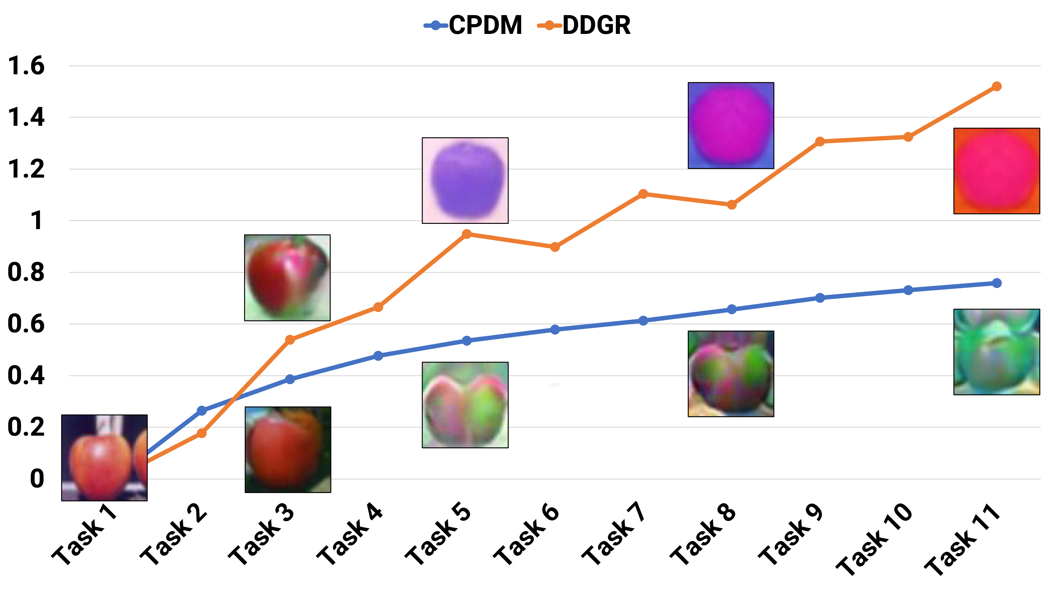
Figure 1: FID scores across tasks for generated images corresponding to the first task dataset of the baselines DDGR [10] and our proposed CPDM. The illustration belongs to the label class “Apple”, whereas the leftmost one is the real photo. As can be observed, for DDGR, the quality of generated apples deteriorates significantly across tasks. Consequently, the generated apples of DDGR in some last tasks become hardly recognizable, while the generated apples of our proposed CPDM maintain their quality more efficiently. Finally, FID scores across tasks for our CPDM are significantly better than DDGR, especially for later tasks when the gap becomes more pronounced.

5.1 Motivations

Catastrophic forgetting (CF) in classifiers poses a significant challenge in TIL. While applying generative models to replay old data can alleviate CF in classifiers, the generative models themselves may face CF within the context of CL. This occurs because, at the end of each task $t$, the generative model is trained based on the new task data $\mathcal{D}^{t}$ and the replay memory $\mathcal{M}^{1:t-1}$. The latter is generated from the generative model trained at the end of task $t-1$, using $\mathcal{D}^{t-1}$ and the previous replay memory $\mathcal{D}^{1:t-2}$. Notably, the quality of old data in the generative replay memory (e.g., $\mathcal{M}^{1}$) diminishes task by task, making it increasingly challenging for current and future diffusion models to maintain high-quality representations on this data.

While it has been demonstrated in [10] that Diffusion Models as generative replay can assist in mitigating the catastrophic forgetting of generative models in CL, our observations indicate that challenges still persist. As illustrated in Figure 1, the quality of generated images for task 1’s data significantly diminishes across tasks. Consequently, the generated images for some of the last tasks exhibit very low quality, making it difficult for the current model to recall old data and exacerbating the issue of catastrophic forgetting.

Our primary approach to alleviate the CF of diffusion models involves learning class prototypes that succinctly summarize data within a given class. Subsequently, during both training and inference of new data, the diffusion models are conditioned on these class prototypes. It is noteworthy that these class prototypes are learnable variables, which serve as a reserved information channel to effectively remind diffusion models of class concepts, contributing to the reduction of CF across tasks.

5.2 Conditional Diffusion Probabilistic Model

In what follows, we present our probabilistic viewpoint of conditional diffusion models.

Forward process. Let $\mathbf{x}_{0}\thicksim q(\mathbf{x}_{0}|y)$ be clean data samples, where $q(\mathbf{x}_{0}|y)$ represents the class-conditional data distribution over $\mathbb{R}^{d}$. Conditioned on $\mathbf{x}_{0}$ and $y$, the joint distribution of the sequence $\mathbf{x}_{1},\mathbf{x}_{2},...,\mathbf{x}_{K}$ can be factorized using the chain rule of probability and the Markov property as follow:

$$q(\mathbf{x}_{1:K}|\mathbf{x}_{0},y)=\Pi_{k=1}^{K}q(\mathbf{x}_{k}|\mathbf{x}_{k-1},y).$$ (5)

Here, $q(\mathbf{x}_{k}|\mathbf{x}_{k-1},y)$ is defined as a Gaussian transition kernel:

$$q(\mathbf{x}_{k}|\mathbf{x}_{k-1},y)=\mathcal{N}\left(\mathbf{x}_{k};\sqrt{\alpha_{k}}\mathbf{x}_{k-1},\left(1-\alpha_{k}\right)\mathbf{I}\right),$$ (6)

where $\alpha_{1}=1$ and $\alpha_{k}\downarrow 0$. Through basic algebraic manipulations, we reach:

$$q(\mathbf{x}_{k}|\mathbf{x}_{0},y)=\mathcal{N}\left(\mathbf{x}_{k};\sqrt{\bar{\alpha}_{k}}\mathbf{x}_{0},\left(1-\bar{\alpha}_{k}\right)\mathbf{I}\right),$$ (7)

where $\bar{\alpha}_{k}=\prod_{i=1}^{k}\alpha_{i}$ rapidly approaches $0$ as $k$ increases. By applying the reparameterization trick, $\mathbf{x}_{k}\sim q(\mathbf{x}_{k}|\mathbf{x}_{0},y)$ suggests that:

$$\mathbf{x}_{k}=\sqrt{\bar{\alpha}_{k}}\mathbf{x}_{0}+\sqrt{1-\bar{\alpha}_{k}}\bm{\epsilon},$$ (8)

where $\mathbf{x}_{0}\sim q(\mathbf{x}_{0}|y)$ and $\bm{\epsilon}\sim\mathcal{N}\left(\mathbf{0},\mathbf{I}\right)$. Eq. (8) enables the sampling of any noisy version $\mathbf{x}_{k}$ from $\mathbf{x}_{0}$. As $K$ becomes sufficiently large, it appears that $\bar{\alpha}_{K}\approx 0$ and $\mathbf{x}_{K}$ seems to be sampled from $\mathcal{N}(\mathbf{0},\mathbf{I})$.

Reverse process. We begin the reverse process with a prior distribution $p(\mathbf{x}_{K}|y)=\mathcal{N}(\mathbf{x}_{K};\mathbf{0},\mathbf{I})$, and then progressively denoise the noisy image $\mathbf{x}_{K}$ to generate new data that belongs to class $y$. The process is encapsulated in the following equation:

$$p_{\theta}(\mathbf{x}_{0:K}|y)=p(\mathbf{x}_{K}|y)\Pi_{k=1}^{K}p_{\theta}(\mathbf{x}_{k-1}|\mathbf{x}_{k},y).$$ (9)

Here, $p_{\theta}(\mathbf{x}_{k-1}|\mathbf{x}_{k},y)$ is a learnable transition kernel. At $k=1$, $\mathbf{x}_{0}\sim p_{\theta}(\mathbf{x}_{0}|\mathbf{x}_{1},y)$ seems to be sampled from $q(\mathbf{x}_{0}|y)$.

Training objective. To learn $p_{\theta}(\mathbf{x}_{k-1}|\mathbf{x}_{k},y)$, we apply the variational approach, represented by minimizing the cross-entropy ($CE$) between $q\left(\mathbf{x}_{0}|y\right)$ and $p_{\theta}\left(\mathbf{x}_{0}|y\right)$:

$$CE\left(q\left(\mathbf{x}_{0}|y\right),p_{\theta}\left(\mathbf{x}_{0}|y\right)\right)=-\mathbb{E}_{q\left(\mathbf{x}_{0}|y\right)}\left[\log p_{\theta}\left(\mathbf{x}_{0}|y\right)\right]$$

$$\leq\mathbb{E}_{q\left(\mathbf{x}_{0:K}|y\right)}\left[\log\frac{q\left(\mathbf{x}_{1:K}\mid\mathbf{x}_{0},y\right)}{p_{\theta}\left(\mathbf{x}_{0:K}|y\right)}\right].$$ (10)

This leads to the optimization problem:

$$\min_{\theta}\mathcal{L}\coloneqq\mathbb{E}_{q\left(\mathbf{x}_{0:K}|y\right)}\left[\log\frac{q\left(\mathbf{x}_{0:K}\mid\mathbf{x}_{0},y\right)}{p_{\theta}\left(\mathbf{x}_{0:K}|y\right)}\right].$$ (11)

We can further derive $\mathcal{L}$ as:

$$\mathcal{L} =\mathbb{E}_{q}\Big{[}\underbrace{D_{KL}\left(q\left(\mathbf{x}_{K}\mid\mathbf{x}_{0},y\right)\|p\left(\mathbf{x}_{K}|y\right)\right)}_{\mathcal{L}_{K}}$$

$$+\sum_{k>1}\underbrace{D_{KL}\left(q\left(\mathbf{x}_{k-1}\mid\mathbf{x}_{k},\mathbf{x}_{0},y\right)\|p_{\theta}\left(\mathbf{x}_{k-1}\mid\mathbf{x}_{k},y\right)\right)}_{\mathcal{L}_{k-1}}$$

$$\underbrace{-\log p_{\theta}\left(\mathbf{x}_{0}\mid\mathbf{x}_{1},y\right)}_{\mathcal{L}_{0}}\Big{]}$$ (12)

(See our supplementary material for more details). While $\mathcal{L}_{K}$ is a constant, $\mathcal{L}_{0}$ is later integrated with $\mathcal{L}_{k-1}$ in the simplified version of the training objective (refer to the optimization problem in Eq. (16)). For $\mathcal{L}_{k-1}$, it is worth noting that $q\left(\mathbf{x}_{k-1}\mid\mathbf{x}_{k},\mathbf{x}_{0},y\right)$ is tractable when conditioned on $\mathbf{x}_{0}$:

$$q\left(\mathbf{x}_{k-1}\mid\mathbf{x}_{k},\mathbf{x}_{0},y\right)=\mathcal{N}\left(\tilde{\bm{\mu}}_{k}\left(\mathbf{x}_{k},\mathbf{x}_{0},y\right),\sigma_{k}^{2}\mathbf{I}\right),$$ (13)

$$\text{where }\tilde{\bm{\mu}}_{k}\left(\mathbf{x}_{k},\mathbf{x}_{0},y\right)=\frac{1}{\sqrt{\alpha_{k}}}\left(\mathbf{x}_{k}-\frac{1-\alpha_{k}}{\sqrt{1-\bar{\alpha}_{k}}}\bm{\epsilon}\right)\,\text{and }$$

$$\sigma_{k}^{2}=\frac{(1-\alpha_{k})(1-\bar{\alpha}_{k-1})}{1-\bar{\alpha}_{k}}.\text{ This hints us to parameterize:}$$

$$p_{\theta}\left(\mathbf{x}_{k-1}\mid\mathbf{x}_{k},y\right)=\mathcal{N}\left(\bm{\mu}_{\theta}\left(\mathbf{x}_{k},k,y\right),\bm{\Sigma}_{\theta}\left(\mathbf{x}_{k},k,y\right)\right),$$ (14)

where $\bm{\mu}_{\theta}\left(\mathbf{x}_{k},k,y\right)=\frac{1}{\sqrt{\alpha_{k}}}\left(\mathbf{x}_{k}-\frac{1-\alpha_{k}}{\sqrt{1-\bar{\alpha}_{k}}}\bm{\epsilon}_{\theta}\left(\mathbf{x}_{k},k,y\right)\right)$, and $\bm{\Sigma}_{\theta}\left(\mathbf{x}_{k},k,y\right)=\sigma_{k}^{2}\mathbf{I}$ is untrained time dependent constants. Therefore, minimizing Kullback–Leibler (KL) divergence in $\mathcal{L}_{k-1}$ leads to training a model $\bm{\mu}_{\theta}$ that predicts $\tilde{\bm{\mu}}_{k}$, which is formulated as:

By applying the reparameterization trick and ignoring the scaling factor, we can further simplify the objective function (15) by learning a network $\bm{\epsilon}_{\theta}(\mathbf{x}_{k},k,y)$ to predict the source noise $\bm{\epsilon}\sim\mathcal{N}\left(\mathbf{0},\mathbf{I}\right)$. The final objective function is as follows:

$$\tilde{\mathcal{L}}_{k-1}=\mathbb{E}_{\bm{\epsilon},\mathbf{x}_{0},k,y}\left[\lVert\bm{\epsilon}-\bm{\epsilon}_{\theta}\left(\mathbf{x}_{k},k,y\right)\rVert^{2}\right],$$ (16)

where $\mathbf{x}_{k}$ is calculated via $\mathbf{x}_{0}$ as described in Eq. (8).

5.3 Class-Prototype Conditional Diffusion Model

Eq. (16) directs us to integrate class-specific information into the diffusion model training. To achieve this, we propose adding class information variables, $\mathbf{c}(y)$ and $\bm{\tau}(y)$, into our conditional diffusion model training process. Consequently, the objective function becomes:

$$\min_{\theta,\mathbf{c}}\mathcal{L}_{DM}\coloneqq\mathbb{E}_{\bm{\epsilon},\mathbf{x}_{0},k,y}\left[\lVert\bm{\epsilon}-\bm{\epsilon}_{\theta}\left(\mathbf{x}_{k},k,\mathbf{c}(y),\bm{\tau}(y)\right)\rVert^{2}\right].$$ (17)

Here, $\mathbf{c}(y)\in\mathbb{R}^{d}$ is a learnable class-prototype designed to capture the most representative features of class $y$. Meanwhile, $\bm{\tau}(y)$ represents the text embedding derived from the CLIP model [27].

5.4 GR with Class-Prototype Conditional Diffusion Model

Training Methodology. For each task $t$, we train the classifier $f^{t}_{\phi}$ by minimizing $CE$ loss w.r.t. $\phi$:

$$\min_{\phi}\mathcal{L_{C}}\coloneqq\mathbb{E}_{(\mathbf{x},y)}\left[CE(f^{t}_{\phi}(\mathbf{x}),y)\right],$$ (18)

where $(\mathbf{x},y)\sim\mathcal{D}^{t}\cup\mathcal{M}^{1:t-1}$. Subsequently, the diffusion model $\bm{\epsilon}^{t}_{\theta}\left(\mathbf{x}_{k},k,\mathbf{c}(y),\bm{\tau}(y)\right)$ learns data from $\mathcal{D}^{t}$ and replay memory $\mathcal{M}^{1:t-1}$ to generate samples for $\mathcal{M}^{1:t}$ that serves for the next task (as illustrated in the left part of Figure 2).

Class-prototype Initialization and Update. At task $t$, for each label $y^{t}_{i}\in\mathcal{Y}^{t}$, we initialize $\mathbf{c}(y^{t}_{i})$ with sample belonging to this label that our model $f^{t}_{\phi}$ has the highest confidence on prediction:

$$\mathbf{c}(y^{t}_{i})\coloneqq\arg\max_{\mathbf{x}^{t}\in\mathcal{X}^{y^{t}_{i}}}p(y^{t}_{i}|\mathbf{x}^{t})=\arg\min_{\mathbf{x}^{t}\in\mathcal{X}^{y^{t}_{i}}}\left[CE(f^{t}_{\phi}(\mathbf{x}^{t}),y^{t}_{i})\right],$$ (19)

where $\mathcal{X}^{y^{t}_{i}}\coloneqq\{\mathbf{x}^{t}|(\mathbf{x}^{t},y^{t})\in\mathcal{D}^{t};y^{t}=y^{t}_{i}\}$. This class prototype is then updated alongside the diffusion model (refer to Eq. (17)).

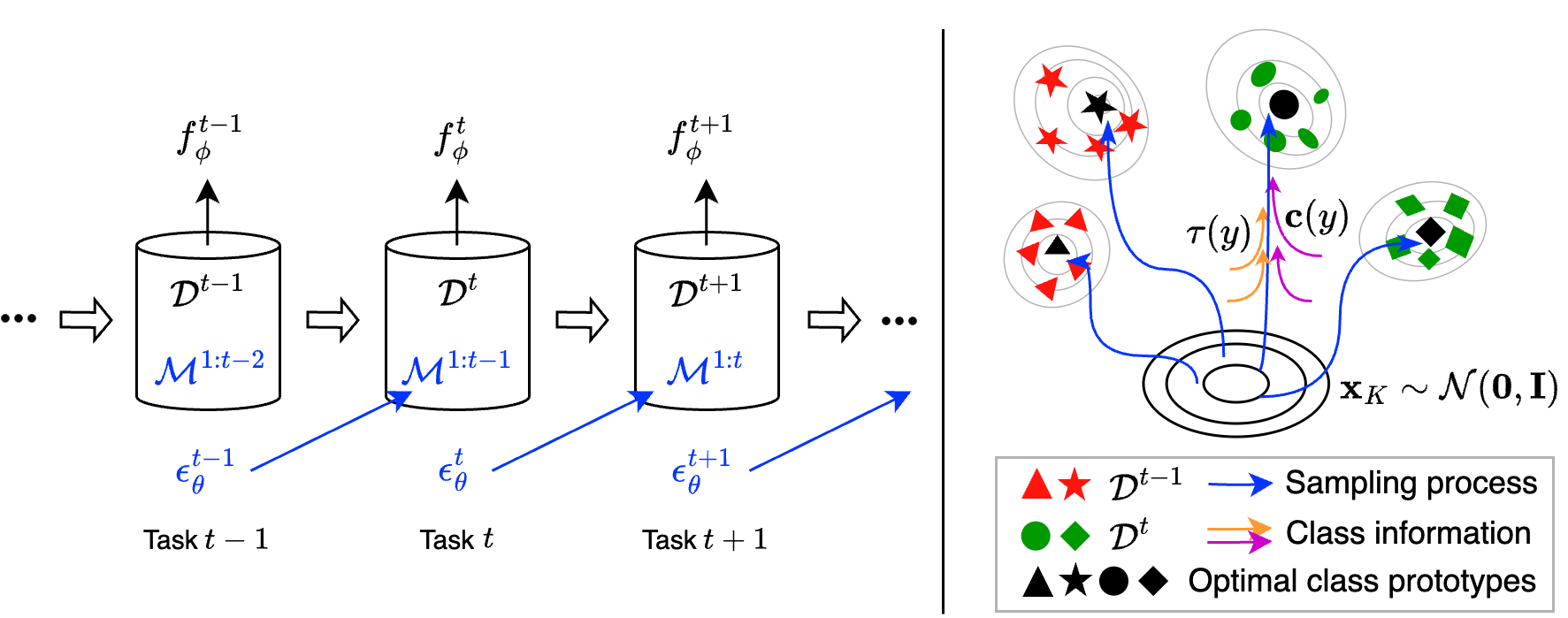
Figure 2: Overall framework of our CPDM for continual learning with generative replay. Left: During task $t$, the classifier $f^{t}_{\phi}$ trains on data from the current task $\mathcal{D}^{t}$ and on data from the previous task $\mathcal{M}^{1:t-1}$ generated by the diffusion model to reduce catastrophic forgetting. Right: The diffusion model begins by denoising the initial noise $\mathcal{N}(\mathbf{0},\mathbf{I})$. Each denoising step incorporates class information from CLIP embeddings $\bm{\tau}(y)$ and the learned class prototype $\mathbf{c}(y)$. The class prototype is designed to capture the most distinctive features of a given class and assists the generator in synthesizing high-quality images.

Diversity Exploration from the Nearest Neighbor. To boost the diversity of generated images, at task $t$, we propose seeking the nearest previous class $\tilde{y}\in\mathcal{Y}^{1:t-1}$ to the current class $y\in\mathcal{Y}^{t}$ by measuring the cosine similarity in CLIP embedding space:

$$\tilde{y}=\arg\max_{\tilde{y}}\dfrac{\bm{\tau}(y)\cdot\bm{\tau}(\tilde{y})}{\lVert\bm{\tau}(y)\rVert\lVert\bm{\tau}(\tilde{y})\rVert}.$$ (20)

To enhance the variety of classes in the current task, we steer the denoising network to predict one of its neighbors, guided by the following objective function:

$$\min_{\theta,\mathbf{c}}\mathcal{L}_{DE}\coloneqq\mathbb{E}_{\mathbf{x}_{0},k,y,\tilde{y}}\big{[}k \lVert\bm{\epsilon}_{\theta}\left(\mathbf{x}_{k},k,\mathbf{c}(y),\bm{\tau}(y)\right)$$

$$-\bm{\epsilon}_{\theta}\left(\mathbf{x}_{k},k,\tilde{\mathbf{c}}(\tilde{y}),\bm{\tau}(\tilde{y})\right)\rVert^{2}\big{]}.$$ (21)

By minimizing this Diversity Exploration (DE) function, the denoising trajectories are guided to align closely with those of their nearest neighbors. Consequently, the diffusion model for the current class is encouraged to synthesize new features inspired by its neighbor, thereby increasing the diversity of the generated samples. Additionally, this method aids in preventing mode collapse and improving the classifier’s generalization capability. The overall objective is then combined into a single function:

$$\min_{\theta,\mathbf{c}}{\mathcal{L}_{DM}+\gamma\mathcal{L}_{DE}},$$ (22)

where $\gamma>0$ adjusts the balance between diverse image generation and high-quality, class-specific image generation. The detailed algorithms are outlined in Algorithms 1 and 2. Finally, a detailed visualization of our CPDM using generative replay is provided in Figure 2.

0:  Task $t$, dataset $\mathcal{D}^{t}$ with labels set $\mathcal{Y}^{t}$, classifier $f_{\phi}$, diffusion model $\bm{\epsilon}_{\theta}$, set of class-prototypes $\mathcal{C}$, drop label rate $\delta$, pretrained CLIP model.

0:  Optimal $\phi^{*}$

1:  for $t=1,...,T$ do

2:     if $t\geq 2$ then

3:        $\mathcal{M}^{1:t-1}=\textit{DiffusionSampler}(\mathcal{Y}^{1:t-1},\mathcal{C}^{1:t-1},\tilde{\bm{\epsilon}}_{\theta})$

4:        $(\mathbf{x},y)\sim\mathcal{D}^{t}\cup\mathcal{M}^{1:t-1}$

5:     else

6:        $(\mathbf{x},y)\sim\mathcal{D}^{t}$

7:     end if

8:     Update $\phi$ according to (18).

9:     $\tilde{\delta}\sim\mathcal{U}(0,1)$

10:     if $\tilde{\delta}\leq\delta$ then

11:        $\bm{\tau}(y)=0$

12:     else

13:        $\bm{\tau}(y)=CLIP(y)$

14:     end if

15:     Initialize $\mathbf{c}(y)$ according to (26).

16:     Update $\theta,\mathbf{c}\in\mathcal{C}^{t}$ according to (22).

17:  end for

Algorithm 1 Pseudocode for training our CPDM.

0:  Label set $\mathcal{Y}^{1:t-1}$, class-prototypes from previous tasks $\mathcal{C}^{1:t-1}$, classifier-free diffusion model $\tilde{\bm{\epsilon}}_{\theta}$, diffusion steps $K$, number of generated samples $L$.

0:  $\mathcal{M}^{t}$

1:  $\mathcal{M}^{t}=\varnothing$

2:  for $y\in\mathcal{Y}^{1:t-1}$ do

3:     $l=0$

4:     while $l\leq L$ do

5:        Get $\mathbf{c}(y)$ from $\mathcal{C}^{1:t-1}$

6:        $\mathbf{x}_{K}\sim\mathcal{N}(\mathbf{0},\mathbf{I})$

7:        for $k=K,...,1$ do

8:           $\mathbf{z}\sim\mathcal{N}(\mathbf{0},\mathbf{I})$

9:           $\tilde{\bm{\mu}}_{\theta}=\frac{1}{\sqrt{\alpha_{k}}}\left(\mathbf{x}_{k}-\frac{1-\alpha_{k}}{\sqrt{1-\bar{\alpha}_{k}}}\tilde{\bm{\epsilon}}_{\theta}\left(\mathbf{x}_{k},k,\mathbf{c}(y),\bm{\tau}(y)\right)\right)$

10:           $\mathbf{x}_{k-1}=\tilde{\bm{\mu}}_{\theta}+\sigma_{k}\mathbf{z}$

11:        end for

12:        $\mathcal{M}^{t}=\mathcal{M}^{t}\cup\{(\mathbf{x}_{0},y)\}$

13:        $l=l+1$

14:     end while

15:  end for

Algorithm 2 DiffusionSampler

6 Experiments

We assess the effectiveness of our proposed CPDM in the commonly encountered Class Incremental Learning (CIL) scenario [35, 36] in CL. Furthermore, we extend our assessment to include another setting, Class Incremental Repeat (CIR) [24, 6], with detailed results and analysis presented in the supplementary materials.

6.1 Setup

To ensure a balanced comparison, we adhere to the four experimental settings outlined in [10], applied to the CIFAR-100 and ImageNet [8] datasets.

Baselines.

We compare our approach with the baselines including Finetuning, SI [39], MAS [2], EWC [19], IMM [21], DGR [33], MeRGAN [5], PASS [41], and DDGR [10]. SI (Synaptic Intelligence), MAS (Memory Aware Synapses), EWC (Elastic Weight Consolidation), and IMM (Incremental Moment Matching) are methods that primarily focus on estimating the prior distribution of model parameters when assimilating new data. Generally, these approaches evaluate the significance of each parameter within a neural network, operating under the assumption of parameter independence for practicality. On the other hand, DGR (Deep Generative Replay) and MeRGAN leverage Generative Adversarial Networks (GANs) to create prior samples, facilitating data replay. Meanwhile, PASS represents a straightforward approach that does not rely on exemplars.

Datasets.

We use two scenarios for each dataset CIFAR-100 and ImageNet. Half of the classes belong to the first task, the rest is divided equally among the remaining tasks. Specific details are as follows:

• CIFAR-100: initial task consists of 50 classes with two cases of incremental tasks: 5 incremental tasks (i.e., 10 classes per task) and 10 incremental tasks (i.e., 5 classes per task)

• ImageNet: initial task consists of 500 classes with two cases of incremental tasks: 5 incremental tasks (i.e., 100 classes per task) and 10 incremental tasks (50 classes per task).

Table 1: Average accuracy and forgetting (%) of methods across 4 benchmark datasets. Underlined scores represent the second-best results.

	Average Accuracy $A_{T}(\uparrow)$								Average Forgetting $F_{T}(\downarrow)$
	CIFAR-100				ImageNet				CIFAR-100				ImageNet
Method	AlexNet		ResNet		AlexNet		ResNet		AlexNet		ResNet		AlexNet		ResNet
	NC=5	10	5	10	50	100	50	100	5	10	5	10	50	100	50	100
Finetuning	6.11	5.12	18.08	17.50	5.33	3.24	12.95	10.28	60.45	59.87	61.65	62.79	56.55	57.83	58.58	59.71
SI	16.96	13.57	26.45	23.15	19.38	14.38	28.88	24.38	48.58	50.18	52.27	56.65	41.18	45.94	41.93	44.56
EWC	15.29	9.71	25.49	18.82	15.22	13.03	23.51	22.03	50.38	54.27	52.83	60.47	45.65	47.01	46.98	46.96
MAS	20.13	18.94	29.94	28.28	16.35	14.51	31.25	25.51	45.75	45.37	49.38	51.31	44.85	45.70	39.55	44.34
IMM	11.26	9.87	21.02	19.79	13.68	11.13	23.19	19.73	54.60	54.57	58.12	59.89	46.65	49.31	47.70	49.62
DGR	42.49	38.16	52.96	48.94	43.94	38.81	53.32	47.56	24.08	26.52	26.36	31.14	17.31	22.52	17.96	21.84
MeRGAN	46.03	43.23	57.19	55.69	—	—	—	—	36.95	26.49	20.12	22.55	—	—	—	—
PASS	53.21	48.65	62.30	60.63	—	—	—	—	27.35	19.43	16.97	21.21	—	—	—	—
DDGR	59.20	52.22	63.40	60.04	53.86	52.21	64.83	61.26	23.00	16.86	15.34	19.25	6.98	7.82	5.65	7.73
CPDM	71.35	61.01	76.56	66.52	58.02	52.46	67.97	65.53	13.80	11.71	10.79	8.73	7.06	4.78	8.52	5.02

Models.

Following previous works [29, 23, 7], two model architectures are used for the classifier: AlexNet [20] and 32-layer ResNet [13]. Similarly, following [16], popular UNet architecture is used for the diffusion model.

Evaluations.

Two common metrics are used to evaluate: Average Accuracy and Average Forgetting during training. Denote $acc_{t}^{i}$ is the accuracy of task $t$ after the model has been trained with task $i$, the metrics of interest can be computed as:

• Average Accuracy at task $i$:

  $$A_{i}=\frac{1}{i}\sum_{t=1}^{i}{acc_{t}^{i}},\forall 1\leq i\leq T$$ (23)

• Average Forgetting at task $i$ $(F_{1}=0)$:

  $$F_{i}=\frac{1}{i-1}\sum_{t=1}^{i-1}{(\max_{1\leq j<i}{acc_{t}^{j}}-acc_{t}^{i})},\forall 2\leq i\leq T$$ (24)

Higher final Average Accuracy $A_{T}(\uparrow)$ and lower final Average Forgetting $F_{T}(\downarrow)$ show better performance of model across all tasks.

6.2 Experimental Results

Table 1 displays the performance of our CPDM compared to baseline models on the CIFAR-100 and ImageNet datasets. The data shows that CPDM surpasses most other models in various tasks on these benchmarks. Specifically, on CIFAR-100, CPDM achieves outstanding results in average accuracy and forgetting, outperforming the baseline in every setting. For instance, under the setting $NC=5$, CPDM attains an average accuracy of $71.35\%$, and a forgetting rate of $13.8\%$, creating a substantial margin of $12.15\%$ in accuracy and $9.2\%$ in forgetting when compared to the top baseline on AlexNet. Similarly, in ResNet, CPDM shows a remarkable improvement of $13.16\%$ in average accuracy for $NC=5$ and $10.52\%$ in forgetting accuracy for $NC=10$. On a more challenging ImageNet dataset, with its $1000$ classes, CPDM also exceeds the best baseline in $6/8$ settings. Notably, with $100$ classes per task, the performance on ResNet is particularly significant, achieving $65.53\%$ in average accuracy and only $5.02\%$ in average forgetting. This is an improvement of $4.27\%$ in accuracy and $2.71\%$ in forgetting compared to the leading baseline DDRG. Additionally, our CPDM also achieved the runner-up score on the remaining 2 tasks. Moreover, CPDM also secures the second-best scores in the remaining two tasks.

6.3 Ablation Study

Catastrophic Forgetting comparison in DMs.

Figure 3 presents the generated images from the CIFAR-100 dataset experiment ($NC=5$), focusing on the initial task. The comparison of our CPDM and DDGR methods highlights a substantial issue. DDGR faces severe challenges with generation catastrophic forgetting, as seen in the later tasks where its generated images become increasingly blurry and difficult to recognize. In contrast, our CPDM effectively maintains key object features, demonstrating a more efficient approach to mitigating generation catastrophic forgetting. This is evident in the clarity and recognizability of the images generated by CPDM, even in successive tasks.

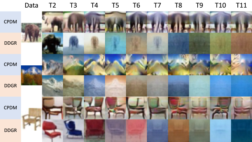
Figure 3: Comparison of generated images from CPDM and DDGR on CIFAR-100

Learning Class-Prototype.

In Figure 4, we present the class-prototypes (on the right) corresponding to the initially most confident images (on the left). Interestingly, the learned class-prototypes appear to emphasize and concentrate more on the foregrounds/objects of the initial images. This focus on foreground information is undoubtedly beneficial for guiding our CPDM to retain the class-concept information in subsequent tasks.

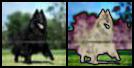
(a)

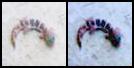
(b)

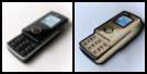
(c)

Figure 4: Class-prototypes before (left) and after learning (right). Object and object boundaries are more focused to better preserve object shape.

Analysis of Class-Prototype Initialization.

In the CIFAR-100 ($NC=5$) experiment using the AlexNet model, we examine the various initializations of the class-prototypes. In addition to the original initialization, given $y^{t}_{i}\in\mathcal{Y}^{t}$, three alternative ones are also investigated as follows:

• Most confident initialization (as presented in Section 5.4).

  $$\mathbf{c}(y^{t}_{i})\coloneqq\arg\max_{\mathbf{x}^{t}\in\mathcal{X}^{y^{t}_{i}}}p(y^{t}_{i}|\mathbf{x}^{t})=\arg\min_{\mathbf{x}^{t}\in\mathcal{X}^{y^{t}_{i}}}\left[CE(f^{t}_{\phi}(\mathbf{x}^{t}),y^{t}_{i})\right].$$ (25)

• Least confident initialization

  $$\mathbf{c}(y^{t}_{i})\coloneqq\arg\min_{\mathbf{x}^{t}\in\mathcal{X}^{y^{t}_{i}}}p(y^{t}_{i}|\mathbf{x}^{t})=\arg\max_{\mathbf{x}^{t}\in\mathcal{X}^{y^{t}_{i}}}\left[CE(f^{t}_{\phi}(\mathbf{x}^{t}),y^{t}_{i})\right].$$ (26)

• Average initialization in the same class

  $$\mathbf{c}(y^{t}_{i})\coloneqq\frac{1}{|\mathcal{X}^{y^{t}_{i}}|}\sum_{\mathbf{x}^{t}\in\mathcal{X}^{y^{t}_{i}}}{\mathbf{x}^{t}}.$$ (27)

• Random initialization

  $$\mathbf{c}(y)\sim\mathcal{N}(\mathbf{0},\mathbf{I})$$ (28)

Figure 5 shows that the most confident initialization achieves the best performance. Meanwhile, starting from random noise provides a slight improvement over DDGR.

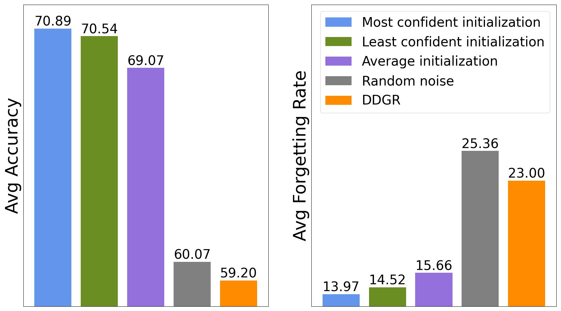
Figure 5: Comparison of final average accuracy $A_{T}(\uparrow)$ and final average forgetting $F_{T}(\downarrow)$ in CIFAR-100 ($NC=5$) with different class-prototype initialization strategies relative to DDGR.

Impact of Nearest Neighbors.

Table 2 shows the effect of the nearest neighbor term. As can be observed, setting $\gamma=1e-4$ helps to improve the performance comparing to without this term. However, setting $\gamma=5e-4$ hurts the performance.

$\gamma$	$0.0$	$1e-4$	$5e-4$
Accuracy	70.89	71.35	67.23
Forget	13.97	13.80	16.75

Table 2: Effect of the nearest neighbors on CIFAR-100.

7 Conclusion

Catastrophic forgetting poses a critical challenge in the realm of continual learning. Generative replay, a method employing a generative model to recreate a replay memory for old tasks, aims to reinforce the classifier’s understanding of past concepts. However, generative models themselves may encounter catastrophic forgetting, impeding the production of high-quality old data across tasks. Recent solutions, such as DDGR, integrating diffusion models, aim to reduce this issue in generation, yet they still face significant challenges. To address this, in this paper, we propose the Class-Prototype conditional Diffusion Model (CPDM) to notably enhance the mitigation of generation catastrophic forgetting. The core idea involves the acquisition of a class-prototype that succinctly encapsulates the characteristics of each class. These class-prototypes then serve as guiding cues for diffusion models, acting as a mechanism to prompt their memory when generating images for earlier tasks. Through empirical experiments on real-world datasets, our CPDM demonstrates its superiority, significantly outperforming current leading methods.

Appendix A Training objective of Conditional Diffusion Probabilistic Model

To learn $p_{\theta}(\mathbf{x}_{k-1}|\mathbf{x}_{k},y)$, we apply the variational approach, which involves minimizing the cross-entropy divergence between $q(\mathbf{x}_{0}|y)$ and $p_{\theta}(\mathbf{x}_{0}|y)$, represented by:

$$CE\left(q\left(\mathbf{x}_{0}|y\right),p_{\theta}\left(\mathbf{x}_{0}|y\right)\right)$$ (29)

$$=-\mathbb{E}_{q\left(\mathbf{x}_{0}|y\right)}\left[\log p_{\theta}\left(\mathbf{x}_{0}|y\right)\right]$$ (30)

$$=-\mathbb{E}_{q\left(\mathbf{x}_{0}|y\right)}\left[\int q\left(\mathbf{x}_{1:K}\mid\mathbf{x}_{0},y\right)\log p_{\theta}\left(\mathbf{x}_{0}|y\right)d\mathbf{x}_{1:K}\right]$$ (31)

$$=-\mathbb{E}_{q\left(\mathbf{x}_{0}|y\right)}\left[\int q\left(\mathbf{x}_{1:K}\mid\mathbf{x}_{0},y\right)\log\frac{p_{\theta}\left(\mathbf{x}_{0:K}|y\right)}{p_{\theta}\left(\mathbf{x}_{1:K}\mid\mathbf{x}_{0},y\right)}d\mathbf{x}_{1:K}\right]$$ (32)

$$=-\mathbb{E}_{q\left(\mathbf{x}_{0}|y\right)}\left[\int q\left(\mathbf{x}_{1:K}\mid\mathbf{x}_{0},y\right)\log\frac{p_{\theta}\left(\mathbf{x}_{0:K}|y\right)}{q\left(\mathbf{x}_{1:K}\mid\mathbf{x}_{0},y\right)}\frac{q\left(\mathbf{x}_{1:K}\mid\mathbf{x}_{0},y\right)}{p_{\theta}\left(\mathbf{x}_{1:K}\mid\mathbf{x}_{0},y\right)}d\mathbf{x}_{1:K}\right]$$ (33)

$$=-\mathbb{E}_{q\left(\mathbf{x}_{0}|y\right)}\left[\int q\left(\mathbf{x}_{1:K}\mid\mathbf{x}_{0},y\right)\log\frac{p_{\theta}\left(\mathbf{x}_{0:K}|y\right)}{q\left(\mathbf{x}_{1:K}\mid\mathbf{x}_{0},y\right)}d\mathbf{x}_{1:K}+D_{KL}\left(q\left(\mathbf{x}_{1:K}\mid\mathbf{x}_{0},y\right)\|p_{\theta}\left(\mathbf{x}_{1:K}\mid\mathbf{x}_{0},y\right)\right)\right]$$ (34)

$$\leq-\mathbb{E}_{q\left(\mathbf{x}_{0}|y\right)}\left[\int q\left(\mathbf{x}_{1:K}\mid\mathbf{x}_{0},y\right)\log\frac{p_{\theta}\left(\mathbf{x}_{0:K}|y\right)}{q\left(\mathbf{x}_{1:K}\mid\mathbf{x}_{0},y\right)}d\mathbf{x}_{1:K}\right]$$ (35)

$$=-\mathbb{E}_{q\left(\mathbf{x}_{0:K}|y\right)}\left[\log\frac{p_{\theta}\left(\mathbf{x}_{0:K}|y\right)}{q\left(\mathbf{x}_{1:K}\mid\mathbf{x}_{0},y\right)}\right]$$ (36)

$$=\mathbb{E}_{q\left(\mathbf{x}_{0:K}|y\right)}\left[\log\frac{q\left(\mathbf{x}_{1:K}\mid\mathbf{x}_{0},y\right)}{p_{\theta}\left(\mathbf{x}_{0:K}|y\right)}\right].$$ (37)

The optimization problem then becomes:

$$\min_{\theta}\mathcal{L}\coloneqq\mathbb{E}_{q\left(\mathbf{x}_{0:K}|y\right)}\left[\log\frac{q\left(\mathbf{x}_{1:K}\mid\mathbf{x}_{0},y\right)}{p_{\theta}\left(\mathbf{x}_{0:K}|y\right)}\right].$$ (38)

We further derive the objective function of interest as:

$$\log\frac{q\left(\mathbf{x}_{1:K}\mid\mathbf{x}_{0},y\right)}{p_{\theta}\left(\mathbf{x}_{0:K}|y\right)} =\log\frac{q\left(\mathbf{x}_{K}\mid\mathbf{x}_{0},y\right)}{p\left(\mathbf{x}_{K},y\right)}\times\prod_{t=2}^{K}\frac{q\left(\mathbf{x}_{k-1}\mid\mathbf{x}_{k},\mathbf{x}_{0},y\right)}{p_{\theta}\left(\mathbf{x}_{k-1}\mid\mathbf{x}_{k},y\right)}\times\frac{1}{p_{\theta}\left(\mathbf{x}_{0}\mid\mathbf{x}_{1},y\right)}$$ (39)

$$=\log\frac{q\left(\mathbf{x}_{K}\mid\mathbf{x}_{0},y\right)}{p\left(\mathbf{x}_{K},y\right)}+\sum_{t=2}^{K}\log\frac{q\left(\mathbf{x}_{k-1}\mid\mathbf{x}_{k},\mathbf{x}_{0},y\right)}{p_{\theta}\left(\mathbf{x}_{k-1}\mid\mathbf{x}_{k},y\right)}-\log p_{\theta}(\mathbf{x}_{0}|\mathbf{x}_{1},y),$$ (40)

leading us to the following conclusion:

$$\mathcal{L} =\mathbb{E}_{q}\left[\log\frac{q\left(\mathbf{x}_{K}\mid\mathbf{x}_{0},y\right)}{p\left(\mathbf{x}_{K}|y\right)}+\sum_{t=2}^{K}\log\frac{q\left(\mathbf{x}_{k-1}\mid\mathbf{x}_{k},\mathbf{x}_{0},y\right)}{p_{\theta}\left(\mathbf{x}_{k-1}\mid\mathbf{x}_{k},y\right)}-\log p_{\theta}(\mathbf{x}_{0}|\mathbf{x}_{1},y)\right]$$ (41)

$$=\mathbb{E}_{q}\Big{[}\underbrace{D_{KL}\left(q\left(\mathbf{x}_{K}\mid\mathbf{x}_{0},y\right)\|p\left(\mathbf{x}_{K}|y\right)\right)}_{\mathcal{L}_{K}}+\sum_{k>1}\underbrace{D_{KL}\left(q\left(\mathbf{x}_{k-1}\mid\mathbf{x}_{k},\mathbf{x}_{0},y\right)\|p_{\theta}\left(\mathbf{x}_{k-1}\mid\mathbf{x}_{k},y\right)\right)}_{\mathcal{L}_{k-1}}$$

$$\underbrace{-\log p_{\theta}\left(\mathbf{x}_{0}\mid\mathbf{x}_{1},y\right)}_{\mathcal{L}_{0}}\Big{]}$$ (42)

Appendix B Implementation Specification and Additional Experimental Results

B.1 Data preparation and preprocessing

In our implementation, which is grounded on the DDGR framework as delineated in [10], a standard preprocessing protocol is employed across three distinct datasets: CIFAR-100, ImageNet, and CORe50 [24]. Central to this protocol is the resizing of image samples to a uniform dimension of $64\times 64$. However, an exception is made for ImageNet, wherein the $64\times 64$ resized samples undergo an additional resizing step, being scaled up to $256\times 256$ before their introduction to the classifier. This resizing process, applied consistently across all datasets, employs a bilinear technique, ensuring uniformity in sample processing.

B.2 Architecture / Hyperparameters

B.2.1 Architecture

We utilize UNet architecture in our implementation. Specifically, we acquire a noisy sample denoted as $\mathbf{x}_{k}$ at time step $k,$ which mirrors the dimensions of real data, measuring $3\times 64\times 64.$ Simultaneously, our class-prototype, $\mathbf{c}(y),$ shares this spatial dimensionality. To facilitate seamless integration into our subsequent processes, we concatenate $\mathbf{x}_{k}$ and $\mathbf{c}(y)$ in the channel dimension, resulting in a composite tensor measuring $6\times 64\times 64.$ This composite tensor is then seamlessly integrated into the UNet model for further processing and analysis. Label text embedding, output of CLIP model, having dimensions of $1\times 768$, is used as key and value of Cross Attention operation in some specific blocks. Figure 6 presents the pipeline of UNet model.

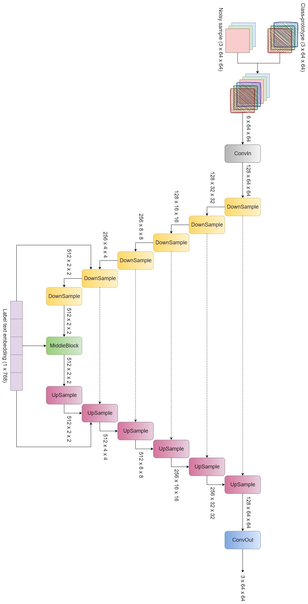
Figure 6: UNet diffusion model.

B.2.2 Label text embeddings

In this section, we detail the method of using text embedding for labels using CLIP.

CI scenario

Two datasets used in this scenario are CIFAR-100 and ImageNet, which have a relatively clear distinction between the classes. Creating label text embedding is as simple as follows:

$$\mathrm{y}\mapsto\bm{\tau}(y)=\mathbf{CLIP}(``\text{a photo of a }[\mathbf{classname}(y)]")$$ (43)

CIR scenario

The CORe50 dataset has a little difference in the meaning of the classes compared to the above two sets. This dataset has a hierarchical labels set, in which there are 10 coarse labels, each includes 5 fine labels. Therefore, label text embedding follows the following formula:

$$\mathrm{y}\mapsto\bm{\tau}(y)=\mathbf{CLIP}(``\text{a photo of a }[\mathbf{classname}(y)]\text{ in category }[\mathbf{classfineindex}(y)]")$$ (44)

where $\mathbf{classname}(\cdot)$ and $\mathbf{classfineindex}(\cdot)$ are presented in the Table 3

Coarse label	Label index $(y)$	Fine label	Class name	Class fine index
plug_adapter	$0$	plug_adapter1	plug adapter	$1$
	$1$	plug_adapter2	plug adapter	$2$
	$2$	plug_adapter3	plug adapter	$3$
	$3$	plug_adapter4	plug adapter	$4$
	$4$	plug_adapter5	plug adapter	$5$
mobile_phone	$5$	mobile_phone1	mobile phone	$1$
	$6$	mobile_phone2	mobile phone	$2$
	$7$	mobile_phone3	mobile phone	$3$
	$8$	mobile_phone4	mobile phone	$4$
	$9$	mobile_phone5	mobile phone	$5$
scissor	$10$	scissor1	scissor	$1$
	$11$	scissor2	scissor	$2$
	$12$	scissor3	scissor	$3$
	$13$	scissor4	scissor	$4$
	$14$	scissor5	scissor	$5$
light_bulb	$15$	light_bulb1	light bulb	$1$
	$16$	light_bulb2	light bulb	$2$
	$17$	light_bulb3	light bulb	$3$
	$18$	light_bulb4	light bulb	$4$
	$19$	light_bulb5	light bulb	$5$
can	$20$	can1	can	$1$
	$21$	can2	can	$2$
	$22$	can3	can	$3$
	$23$	can4	can	$4$
	$24$	can5	can	$5$
glass	$25$	glass1	glass	$1$
	$26$	glass2	glass	$2$
	$27$	glass3	glass	$3$
	$28$	glass4	glass	$4$
	$29$	glass5	glass	$5$
ball	$30$	ball1	ball	$1$
	$31$	ball2	ball	$2$
	$32$	ball3	ball	$3$
	$33$	ball4	ball	$4$
	$34$	ball5	ball	$5$
marker	$35$	marker1	marker	$1$
	$36$	marker2	marker	$2$
	$37$	marker3	marker	$3$
	$38$	marker4	marker	$4$
	$39$	marker5	marker	$5$
cup	$40$	cup1	cup	$1$
	$41$	cup2	cup	$2$
	$42$	cup3	cup	$3$
	$43$	cup4	cup	$4$
	$44$	cup5	cup	$5$
remote_control	$45$	remote_control1	remote control	$1$
	$46$	remote_control2	remote control	$2$
	$47$	remote_control3	remote control	$3$
	$48$	remote_control4	remote control	$4$
	$49$	remote_control5	remote control	$5$

Table 3: Details CORe50 dataset labels.

B.2.3 Hyperparameters

Details of hyperparameters for each experiment are shown in Table 4.

Scenario			CI				CIR
Dataset			CIFAR-100		ImageNet		CORe50
Experiment			$NC=5$	$NC=10$	$NC=50$	$NC=100$
Statistic	No. tasks		$11$	$6$	$11$	$6$	$79$
	No. classes/task	Initial task	$50$	$50$	$500$	$500$	$10$
		Rest tasks	$5$	$10$	$50$	$100$	$5$
	No. training samples/task	Initial task	$25000$	$25000$	$650000$	$650000$	$3000$
		Rest tasks	$2500$	$5000$	$130000$	$65000$	$1500$
Classifier	No. training epochs/task		$100$	$100$	$30$	$30$	$100$
	Batch size		$256$	$256$	$64$	$64$	$256$
	Optimizer		SGD	SGD	SGD	SGD	SGD
	Learning rate		$0.001$	$0.001$	$0.0001$	$0.0001$	$0.0001$
	Weight decay		$0.0005$	$0.0005$	$0.0005$	$0.0005$	$0.0005$
Diffusion	Diversity Exploration weight $(\gamma)$		$0.0001$	$0.0001$	$0.0001$	$0.0001$	$0.0$
	No. training steps/task	Initial task	$15000$	$15000$	$150000$	$150000$	$15000$
		Rest tasks	$15000$	$15000$	$30000$	$60000$	$15000$
	Batch size		$64$	$64$	$64$	$64$	$64$
	Mixed precision		fp16	fp16	fp16	fp16	fp16
	Drop label rate (Classifier-free guidance)		$0.2$	$0.2$	$0.2$	$0.2$	$0.2$
	Optimizer		AdamW	AdamW	AdamW	AdamW	AdamW
	Learning rate		$0.0001$	$0.0001$	$0.0001$	$0.0001$	$0.0001$
	Weight decay		$0.01$	$0.01$	$0.01$	$0.01$	$0.01$
	Gradient clipping		$1.0$	$1.0$	$1.0$	$1.0$	$1.0$
	Training scheduler		DDPM	DDPM	DDPM	DDPM	DDPM
	No. training timesteps		$1000$	$1000$	$1000$	$1000$	$1000$
	Inference scheduler		DDIM	DDIM	DDIM	DDIM	DDIM
	No. inference timesteps		$100$	$100$	$100$	$100$	$100$
	Classifier-free guidance sampling weight ($w$)		$4.0$	$4.0$	$4.0$	$4.0$	$4.0$
	No. generated samples/class		$20$	$20$	$20$	$20$	$20$
Class-prototype	Learning rate		$0.01$	$0.01$	$0.01$	$0.01$	$0.01$
	Weight decay		$0.01$	$0.01$	$0.01$	$0.01$	$0.01$

Table 4: Details of hyperparameters.

B.3 Additional experiments

B.3.1 Result in CIR scenario

In our study, we applied our methodology in the Class Incremental Learning with Repetition (CIR) framework, utilizing the CORe50 dataset as the basis for our experiments. The CORe50 dataset is comprised of ten primary categories, each subdivided into five subclasses. We approached the dataset with a ‘batch’ based task splitting methodology, resulting in a total of 79 distinct tasks. The initial task encompasses ten classes, each with 3,000 samples, while each of the subsequent 78 tasks includes five classes with 1,500 samples per task. A singular, fixed test set comprising 44,972 samples was employed consistently across all tasks. The final accuracy results obtained on this test set are detailed in Table 5 in our findings. Our method achieves results approximating DDGR in experiments with the AlexNet model, while also significantly outperforming ($8.03$ for $A_{T}$) with ResNet32.

Model architecture		AlexNet		ResNet32
Metric		$A_{T}(\uparrow)$	$\max_{1\leq i\leq T}(A_{i})(\uparrow)$	$A_{T}(\uparrow)$	$\max_{1\leq i\leq T}(A_{i})(\uparrow)$
Method	DDGR	$\approx 31.00$	$<32.00$	$40.66$	$<44.00$
	CPDM	$31.05$	34.30	48.69	53.31

Table 5: Accuracy (final and max values) on CORe50 dataset in CIR scenario.

B.3.2 Experiment without a large first task

Table 6 presents the Average Accuracy after each task on CIFAR-100 where all tasks have the same number of classes ($20$) with AlexNet as classifier architecture. Our method yields better results compared to DDGR and PASS across all tasks, however the gap about the final Average Accuracy $(5.14)$ is not as much as in other cases which have a large first task $(NC=5:\text{ }12.15,\text{ }NC=10:\text{ }8.79)$. There are two reasons: fewer tasks are considered, and the capacity of the first task is smaller. Hence, it becomes simpler for the classifier to remember old tasks.

Average Accuracy		Task $1$ ($A_{1}$)	Task $2$ ($A_{2}$)	Task $3$ ($A_{3}$)	Task $4$ ($A_{4}$)	Task $5$ ($A_{5}$)
Method	PASS	$70.51$	$52.17$	$50.41$	$47.39$	$44.32$
	DDGR	70.65	54.33	53.35	51.16	49.03
	CPDM	71.15	61.30	59.52	56.88	54.17

Table 6: Average Accuracy $A_{i}(\uparrow)$ across tasks on CIFAR-100 $5$ tasks, $20$ classes / task, AlexNet model.

B.3.3 The effect of diffusion steps

Increasing the number of diffusion timesteps $(K)$ in training (from $1000$ to $2000$, $3000$, $4000$) while keeping the number of training steps and the number of inference timesteps $(100)$ makes the generator converge more slowly and make it more difficult to form an image, thereby making the results worse. Table 7 shows final Average Accuracy and final Average Forgetting of AlexNet model for CIFAR-100 dataset in two cases $NC=5$ and $NC=10$.

No. timesteps $(K)$	$A_{T}(\uparrow)$		$F_{T}(\downarrow)$
	$NC=5$	$NC=10$	$NC=5$	$NC=10$
$1000$	$71.35$	$61.01$	$13.80$	$11.71$
$2000$	$67.06$	$55.18$	$17.77$	$17.01$
$3000$	63.23	$53.36$	21.02	$19.28$
$4000$	58.46	$46.79$	25.91	$24.29$

Table 7: Results on CIFAR-100, AlexNet model, while changing the number of diffusion timesteps.

References

- Achille et al. [2018] Alessandro Achille, Tom Eccles, Loic Matthey, Christopher P Burgess, Nick Watters, Alexander Lerchner, and Irina Higgins. Life-long disentangled representation learning with cross-domain latent homologies. In Proceedings of the 32nd International Conference on Neural Information Processing Systems, page 9895–9905, 2018.
- Aljundi et al. [2018] Rahaf Aljundi, Francesca Babiloni, Mohamed Elhoseiny, Marcus Rohrbach, and Tinne Tuytelaars. Memory aware synapses: Learning what (not) to forget. In Proceedings of the European conference on computer vision (ECCV), pages 139–154, 2018.
- Chaudhry et al. [2019a] Arslan Chaudhry, Marc’Aurelio Ranzato, Marcus Rohrbach, and Mohamed Elhoseiny. Efficient lifelong learning with a-GEM. In International Conference on Learning Representations, 2019a.
- Chaudhry et al. [2019b] Arslan Chaudhry, Marcus Rohrbach, Mohamed Elhoseiny, Thalaiyasingam Ajanthan, Puneet K Dokania, Philip HS Torr, and M Ranzato. Continual learning with tiny episodic memories. 2019b.
- Chenshen et al. [2018] WU Chenshen, L Herranz, LIU Xialei, et al. Memory replay gans: Learning to generate images from new categories without forgetting [c]. In The 32nd International Conference on Neural Information Processing Systems, Montréal, Canada, pages 5966–5976, 2018.
- Cossu et al. [2021] Andrea Cossu, Gabriele Graffieti, Lorenzo Pellegrini, Davide Maltoni, Davide Bacciu, Antonio Carta, and Vincenzo Lomonaco. Is class-incremental enough for continual learning?, 2021.
- De Lange et al. [2021] Matthias De Lange, Rahaf Aljundi, Marc Masana, Sarah Parisot, Xu Jia, Alevs Leonardis, Gregory Slabaugh, and Tinne Tuytelaars. A continual learning survey: Defying forgetting in classification tasks. IEEE transactions on pattern analysis and machine intelligence, 44(7):3366–3385, 2021.
- Deng et al. [2009] Jia Deng, Wei Dong, Richard Socher, Li-Jia Li, Kai Li, and Li Fei-Fei. Imagenet: A large-scale hierarchical image database. In 2009 IEEE conference on computer vision and pattern recognition, pages 248–255. Ieee, 2009.
- French [1999] Robert M French. Catastrophic forgetting in connectionist networks. Trends in cognitive sciences, 3(4):128–135, 1999.
- Gao and Liu [2023] Rui Gao and Weiwei Liu. DDGR: Continual learning with deep diffusion-based generative replay. In Proceedings of the 40th International Conference on Machine Learning, pages 10744–10763, 2023.
- Goodfellow et al. [2014] Ian Goodfellow, Jean Pouget-Abadie, Mehdi Mirza, Bing Xu, David Warde-Farley, Sherjil Ozair, Aaron Courville, and Yoshua Bengio. Generative adversarial nets. In Advances in Neural Information Processing Systems. Curran Associates, Inc., 2014.
- Goodfellow [2016] Ian J. Goodfellow. Nips 2016 tutorial: Generative adversarial networks. ArXiv, abs/1701.00160, 2016.
- He et al. [2016] Kaiming He, Xiangyu Zhang, Shaoqing Ren, and Jian Sun. Deep residual learning for image recognition. In Proceedings of the IEEE conference on computer vision and pattern recognition, pages 770–778, 2016.
- Ho and Salimans [2021] Jonathan Ho and Tim Salimans. Classifier-free diffusion guidance. In NeurIPS 2021 Workshop on Deep Generative Models and Downstream Applications, 2021.
- Ho et al. [2020a] Jonathan Ho, Ajay Jain, and Pieter Abbeel. Denoising diffusion probabilistic models. In Advances in Neural Information Processing Systems, pages 6840–6851. Curran Associates, Inc., 2020a.
- Ho et al. [2020b] Jonathan Ho, Ajay Jain, and Pieter Abbeel. Denoising diffusion probabilistic models. Advances in neural information processing systems, 33:6840–6851, 2020b.
- Kemker and Kanan [2018] Ronald Kemker and Christopher Kanan. Fearnet: Brain-inspired model for incremental learning. In International Conference on Learning Representations, 2018.
- Kingma and Welling [2014] Diederik P. Kingma and Max Welling. Auto-encoding variational bayes. In 2nd International Conference on Learning Representations, ICLR 2014, Banff, AB, Canada, April 14-16, 2014, Conference Track Proceedings, 2014.
- Kirkpatrick et al. [2017] James Kirkpatrick, Razvan Pascanu, Neil Rabinowitz, Joel Veness, Guillaume Desjardins, Andrei A Rusu, Kieran Milan, John Quan, Tiago Ramalho, Agnieszka Grabska-Barwinska, et al. Overcoming catastrophic forgetting in neural networks. Proceedings of the national academy of sciences, 114(13):3521–3526, 2017.
- Krizhevsky et al. [2012] Alex Krizhevsky, Ilya Sutskever, and Geoffrey E Hinton. Imagenet classification with deep convolutional neural networks. Advances in neural information processing systems, 25, 2012.
- Lee et al. [2017] Sang-Woo Lee, Jin-Hwa Kim, Jaehyun Jun, Jung-Woo Ha, and Byoung-Tak Zhang. Overcoming catastrophic forgetting by incremental moment matching. Advances in neural information processing systems, 30, 2017.
- Li and Hoiem [2017] Zhizhong Li and Derek Hoiem. Learning without forgetting. IEEE transactions on pattern analysis and machine intelligence, 40(12):2935–2947, 2017.
- Liu et al. [2020] Yaoyao Liu, Yuting Su, An-An Liu, Bernt Schiele, and Qianru Sun. Mnemonics training: Multi-class incremental learning without forgetting. In Proceedings of the IEEE/CVF conference on Computer Vision and Pattern Recognition, pages 12245–12254, 2020.
- Lomonaco and Maltoni [2017] Vincenzo Lomonaco and Davide Maltoni. Core50: a new dataset and benchmark for continuous object recognition, 2017.
- Mallya and Lazebnik [2018] Arun Mallya and Svetlana Lazebnik. Packnet: Adding multiple tasks to a single network by iterative pruning. In 2018 IEEE/CVF Conference on Computer Vision and Pattern Recognition, pages 7765–7773, 2018.
- Mundt et al. [2022] Martin Mundt, Iuliia Pliushch, Sagnik Majumder, Yongwon Hong, and Visvanathan Ramesh. Unified probabilistic deep continual learning through generative replay and open set recognition. Journal of Imaging, 8(4):93, 2022.
- Radford et al. [2021] Alec Radford, Jong Wook Kim, Chris Hallacy, Aditya Ramesh, Gabriel Goh, Sandhini Agarwal, Girish Sastry, Amanda Askell, Pamela Mishkin, Jack Clark, Gretchen Krueger, and Ilya Sutskever. Learning transferable visual models from natural language supervision. In Proceedings of the 38th International Conference on Machine Learning, pages 8748–8763. PMLR, 2021.
- Ramapuram et al. [2020] Jason Ramapuram, Magda Gregorova, and Alexandros Kalousis. Lifelong generative modeling. Neurocomputing, 404:381–400, 2020.
- Rebuffi et al. [2017] Sylvestre-Alvise Rebuffi, Alexander Kolesnikov, Georg Sperl, and Christoph H Lampert. icarl: Incremental classifier and representation learning. In Proceedings of the IEEE conference on Computer Vision and Pattern Recognition, pages 2001–2010, 2017.
- Robins [1995] Anthony Robins. Catastrophic forgetting, rehearsal and pseudorehearsal. Connection Science, 7(2):123–146, 1995.
- Saha et al. [2021] Gobinda Saha, Isha Garg, and Kaushik Roy. Gradient projection memory for continual learning. In International Conference on Learning Representations, 2021.
- Serra et al. [2018] Joan Serra, Didac Suris, Marius Miron, and Alexandros Karatzoglou. Overcoming catastrophic forgetting with hard attention to the task. In Proceedings of the 35th International Conference on Machine Learning, pages 4548–4557. PMLR, 2018.
- Shin et al. [2017] Hanul Shin, Jung Kwon Lee, Jaehong Kim, and Jiwon Kim. Continual learning with deep generative replay. In Advances in Neural Information Processing Systems. Curran Associates, Inc., 2017.
- Sohl-Dickstein et al. [2015] Jascha Sohl-Dickstein, Eric Weiss, Niru Maheswaranathan, and Surya Ganguli. Deep unsupervised learning using nonequilibrium thermodynamics. In International conference on machine learning, pages 2256–2265. PMLR, 2015.
- Van de Ven and Tolias [2018] Gido M Van de Ven and Andreas S Tolias. Generative replay with feedback connections as a general strategy for continual learning. arXiv preprint arXiv:1809.10635, 2018.
- Van de Ven and Tolias [2019] Gido M Van de Ven and Andreas S Tolias. Three scenarios for continual learning. arXiv preprint arXiv:1904.07734, 2019.
- Wu et al. [2018] Chenshen Wu, Luis Herranz, Xialei Liu, Yaxing Wang, Joost van de Weijer, and Bogdan Raducanu. Memory replay gans: Learning to generate images from new categories without forgetting. In Proceedings of the 32nd International Conference on Neural Information Processing Systems, page 5966–5976, 2018.
- Xu and Zhu [2018] Ju Xu and Zhanxing Zhu. Reinforced continual learning. In Proceedings of the 32nd International Conference on Neural Information Processing Systems, page 907–916, 2018.
- Zenke et al. [2017] Friedemann Zenke, Ben Poole, and Surya Ganguli. Continual learning through synaptic intelligence. In International conference on machine learning, pages 3987–3995. PMLR, 2017.
- Zhai et al. [2019] Mengyao Zhai, Lei Chen, Frederick Tung, Jiawei He, Megha Nawhal, and Greg Mori. Lifelong gan: Continual learning for conditional image generation. In Proceedings of the IEEE/CVF international conference on computer vision, pages 2759–2768, 2019.
- Zhu et al. [2021] Fei Zhu, Xu-Yao Zhang, Chuang Wang, Fei Yin, and Cheng-Lin Liu. Prototype augmentation and self-supervision for incremental learning. In Proceedings of the IEEE/CVF Conference on Computer Vision and Pattern Recognition, pages 5871–5880, 2021.
Supplementary Material for