[1]organization=National Superconducting Cyclotron Laboratory, Michigan State University, East Lansing, Michigan 48824, USA
[3]organization=Department of Physics, Michigan State University, East Lansing, Michigan 48824, USA \affiliation[KENT]organization=Kent State University, 800 E Summit St, Kent, Ohio, 44240, USA \affiliation[2]organization=RIKEN Nishina Center, Hirosawa 2-1, Wako, Saitama 351-0198, Japan
[4]organization=China Institute of Atomic Energy; Beijing, 102413, PR China
[5]organization=Department of Physics, Kyoto University, Kita-shirakawa, Kyoto 606-8502, Japan
[6]organization=Department of Physics, Korea University, Seoul 02841, Republic of Korea
[7]organization=Institut für Kernphysik, Technische Universität Darmstadt, D-64289 Darmstadt, Germany \affiliation[8]organization=GSI Helmholtzzentrum für Schwerionenforschung, Planckstrasse 1, 64291 Darmstadt, Germany
[10]organization=Faculty of Physics, Astronomy and Applied Computer Science, Jagiellonian University, Kraków, Poland
[9]Division of Experimental Physics, Rudjer Boskovic Institute, Zagreb, Croatia
[12]organization=Department of Physics, Rikkyo University, Nishi-Ikebukuro 3-34-1, Tokyo 171-8501, Japan
[13]organization=Rare Isotope Science Project, Institute for Basic Science, Daejeon 34047, Republic of Korea
[14]organization=Department of Physics, Tohoku University, Sendai 980-8578, Japan
[15]organization=Department of Physics, Tokyo Institute of Technology, Tokyo 152-8551, Japan
[11]organization=Institute of Nuclear Physics PAN, ul. Radzikowskiego 152, 31-342 Kraków, Poland
[16]organization=Cyclotron Institute, Texas A&M University, College Station, Texas 77843, USA
[17]organization=Nikhef National Institute for Subatomic Physics, Amsterdam, Netherlands
[KMUT]Department of Physics, Faculty of Science, King Mongkut’s University of Technology Thonburi, Bangkok, Thailand \affiliation[TACS]Center of Excellence in Theoretical and Computational Science (TACS-CoE), Faculty of Science, King Mongkut’s University of Technology Thonburi, Bangkok, Thailand
[18]organization=Department of Physics, Tsinghua University, Beijing 100084, PR China
[19]organization=Department of Chemistry, Texas A&M University, College Station, Texas 77843, USA
Constraining nucleon effective masses with flow and stopping observables from the SRIT experiment
Abstract
Properties of the nuclear equation of state (EoS) can be probed by measuring the dynamical properties of nucleus-nucleus collisions. In this study, we present the directed flow (), elliptic flow () and stopping (VarXZ) measured in fixed target Sn + Sn collisions at with the SRIT Time Projection Chamber. We perform Bayesian analyses in which EoS parameters are varied simultaneously within the Improved Quantum Molecular Dynamics-Skyrme (ImQMD-Sky) transport code to obtain a multivariate correlated constraint. The varied parameters include symmetry energy, , and slope of the symmetry energy, , at saturation density, isoscalar effective mass, , isovector effective mass, and the in-medium cross-section enhancement factor . We find that the flow and VarXZ observables are sensitive to the splitting of proton and neutron effective masses and the in-medium cross-section. Comparisons of ImQMD-Sky predictions to the SRIT data suggest a narrow range of preferred values for , and .
1 Introduction
Nuclear matter is a significant component of neutron stars, and understanding its properties can elucidate many features of these celestial objects. Calculating the properties of both nuclear matter and neutron stars requires extensive knowledge of the nuclear equation of state (EoS), which describes the dependence of nuclear-matter internal energy on various state variables. Progress in understanding nuclear EoS has been achieved through heavy ion collisions [1, 2, 3] and multimessenger astronomical observations of neutron stars [4, 5, 6, 7, 8, 9, 10, 11, 12, 13, 14, 15, 16, 17, 18]. In this paper, we present new experimental results on flow and stopping measurements from the SRIT heavy ion collision experiment. Multiple observables are analyzed simultaneously using Bayesian inference to investigate correlations between various EoS parameters.
This paper is organized as follows: Section 2 provides a brief overview of the nuclear EoS and relevant parameters. This is followed by a discussion of the experimental setup and the selection of observables in Section 3. The transport model and Bayesian inference are discussed in Section 4. The experimental measurements and posterior constraints on EoS parameters are reported in Section 5, and finally, a summary is given in Section 6.
2 Nuclear equation of state
Nuclear EoS is a function of baryon number density and asymmetry , where represents the difference in neutron () and proton () number densities divided by total density . We write the nuclear EoS as the sum of an isoscalar term and an isovector term , i.e. + . The first term, , is the energy per nucleon of nuclear matter with equal proton and neutron densities (); it provides the EoS of symmetric nuclear matter (SNM). The second term describes how the energy changes as a function of neutron-proton asymmetry. It can be approximately written as , where describes the dependence of nuclear EoS on neutron excess at different densities and is called the symmetry energy term. We truncate the expansion in at second order because the next (fourth) order term in contributes negligibly at asymmetries achieved in low energy nuclear collisions [19].
Many current heavy-ion collision efforts have focused on constraining the first few coefficients in a Taylor expansion of around saturation density, . Such expansions are commonly parameterized by,
| (1) |
where and , and are labels given to the first three expansion coefficients that describe the energy, slope and curvature of the EOS at saturation density, respectively. Similarly, the isoscalar term is commonly parameterized as,
| (2) |
where and are labels given to the first two non-zero expansion coefficients. From masses and other nuclide properties, the saturation energy for symmetric nuclear matter has been determined to be [6]. Experiments that measured Giant Monopole resonances suggest that [6].
Theoretical analysis has found that the form of momentum-dependent potential also affects [20]. This momentum dependence can be quantified by ratios of the isoscalar effective mass, , and isovector effective mass, , to the mass of a nucleon, , in free space. The isoscalar effective mass comes from the isoscalar part of the momentum dependent mean field potential [20]. In asymmetric matter, the strength of the neutron and proton effective mass splitting is related to the momentum dependence of the isovector mean-field potential. [21, 22, 23]. Near , this splitting is related to the isovector effective mass , where is the enhancement factor of the Thomas-Reiche-Kuhn sum rule [20, 24].
The difference between the proton and neutron effective mass splitting, , can be calculated from and with the following formula [25],
| (3) |
Recent measurements and analysis from the SRIT experiment obtained a two-dimensional constraint on and through pion spectral ratio [15]. The yield ratio of to spectra is used to derive this constraint because both and influence the nucleon momenta; quantifies the isospin dependent contribution to the nucleon potential energy and quantifies the isospin dependent impact on the nucleon kinetic energy. Either increasing or decreasing will increase the energies of neutrons relative to protons. This increases the numbers of n-n collisions relative to p-p collisions at energies above the pion production threshold and enhances the production of relative to that of .
3 Experimental setup and observable selection
3.1 Experimental setup
In the SRIT experiment, we bombarded isotopically enriched 112Sn and 124Sn targets with secondary radioactive 108Sn and 132Sn beams and also stable 112Sn and 124S beams at . The targets were placed at the entrance of the SRIT Time Projection Chamber (TPC), which was installed inside the SAMURAI dipole magnet [26, 27] at the Radioactive Isotope Beam Factory (RIBF). The SRIT TPC identified and measured the momenta of charged particles [28, 27, 29, 26] produced in 108SnSn, 112SnSn, 124SnSn and 132Sn +124Sn collisions. Some results for the production of pions, hydrogen and helium isotopes have been previously published [30, 15, 31, 32]. In this paper, we present analyses of collective flow and stopping from this experiment.
3.2 Observable selection
Collective flow is a descriptive label for a group of observables that have been widely used to constrain the nuclear EoS using heavy ion collisions [4, 33, 34, 35, 36, 18, 37]. It often involves analyses of anisotropies in the azimuthal distributions of emitted particles with respect to the reaction plane. Such collective flow observables in nucleus-nucleus collisions commonly reflect the pressures on participant nucleons in the overlapping region of projectile and target wherein this participant matter is compressed. Flow observables also reflect the presence of spectator nucleons that reside outside of the participant region and block the escape of participant nucleons from the compressed participant region.
Flow is a promising observable to constrain nuclear EoS because of its correlation with nuclear pressure. If the mean field is highly repulsive, participant nucleons experience higher pressures which leads to early emission, but this emission is partially blocked by the spectator nucleons if they have not already moved past the participant region before it can expand into the spectator matter [4, 38, 39]. The blocking of the expanding participant matter by the spectator nucleons results in azimuthal anisotropies in fragment emissions. In very central collisions, there is very little spectator matter so emitted particles exhibit little anisotropies. With increasing impact parameter, the amount of spectator matter increases and the importance of the spectators blocking the emitted particles results in the increasing directional dependence that is characteristic of the directed flow.
Collective flow can be quantified by the Fourier coefficients of the fragments’ azimuthal distributions with respect to the azimuthal angle for the reaction plane [40],
| (4) |
In the above equation, is the particle yield, is the azimuthal angle of emission for the particle, is called the directed flow and is called the elliptic flow. Experimentally, and are calculated by the following formula,
| (5) |
In this paper, we determined the azimuthal angle of the reaction plane experimentally with the Q-vector method [41]. Q-vector is defined as,
| (6) |
where is a unit vector pointing in the direction of the transverse momentum of the track, is the particle’s rapidity in the C.M. frame () normalized by beam rapidity in the nucleon-nucleon frame (), and sign is the sign function. We are free to choose the weighting factor , with common choices including or . The effect of using different will be considered as systematic uncertainty. The reaction plane angle is chosen by the azimuthal angle of . Although this approximation and the limited detector acceptance causes non-negligible broadening in the reaction plane resolution, appropriate formulas are used to correct for these effects. For details on these corrections, please refer to Ref. [41]. In this manuscript, we report only the flow values that have been corrected.
Equation (5) can be calculated by averaging over fragments of the same species. Both the theoretical and experimental values of and depend on the mass and species of each fragment, but the probability of producing a cluster of a particular mass depends on the details of the clusterization mechanism of each transport model. The underlying physics of this process is not accurately calculated by most transport codes [42, 43], and this can result in significant systematic uncertainties in theoretical predictions of flow for different isotopes.
To compute light fragments, such as deuterons, tritons, and helium from final nucleon distribution from transport models, various cluster recognition methods have been employed, such as the minimum spanning tree method used in QMD type models [44]. This method classifies neutrons and protons that are emitted at small relative distances and momenta as heavy clusters. [44]. However, this process has a model dependence that reflects the influence of long-range multi-particle correlations that are not yet fully understood [42, 43]. As a result, isotope-specific observable heavily depends on a detailed understanding of clusterization, and transport model predictions for these observables can often be unreliable.
To construct an observable that does not require an accurate description of the clusterization process, we calculate the Coalescence Invariant flow (C.I. flow) distributions. These distributions approximate the flow of nucleons prior to cluster formation by including contributions from p, d, t,3He and 4He together in the calculation of averages of cosines in Eq. (5). Each fragment is weighted by their number of protons, i.e. Helium isotopes are weighted twice as much as Hydrogen isotopes. Fragments heavier than 4He are not included due to their low yields.
We select the impact parameter with gates on total detected charged particle multiplicity as described in Ref. [26]. This centrality selection method was also used in our previous SRIT publications [30, 15, 31]. Due to the limited geometric acceptance in the SRIT TPC, nuclear fragments with large momenta emitted at backward angles in the C.M. frame cannot be efficiently detected, so we limit our flow data to .
In addition to the mean field potentials in the EoS, momentum transfers that contribute to collective flow are also influenced by the in-medium nucleon-nucleon (NN) cross-section [45, 46]. We construct the stopping observable, VarXZ=VarX/VarZ, where VarX and VarZ are the variances of particle rapidity distributions in the transverse and longitudinal directions, respectively. Since VarXZ is a ratio of variances, much of the systematic error from clusterization is cancelled out in the division. VarXZ measures the degree of stopping and thermalization [47], and has also been used to probe the nuclear shear viscosity [48]. It is closely influenced by the in-medium cross-section [47].
To reconstruct this observable and calculate the momentum of the particles accurately, only tracks emitted nearly perpendicular to the magnetic field of the TPC are used. Based on the performance of the SRIT TPC [49], azimuth cuts of , and are used for this purpose. These cuts are also used in the other SRIT analyses [30, 15, 50, 32]. Since determination of the reaction plane does not require as precise values for the magnitude of the momenta of particles, and to minimize bias due to particle cut, we do not impose these restrictive cuts in azimuthal angle on particles in calculating azimuthal orientation of the reaction plane.
The -axis in VarX can be any arbitrary laboratory axis that is perpendicular to the beam axis, consistent with definitions in Ref. [47]. Given the arbitrary azimuthal orientation of the -axis for the VarX observable, we can and do calculate -rapidity distribution by projecting of each track onto planes with random azimuthal angles.
SRIT TPC cannot efficiently measure fragments at so data is not available at all rapidities for 108SnSn and 132SnSn reactions, individually. However, we have constructed the full rapidity distribution of 112SnSn by combining the results of 112SnSn and 124SnSn reactions. Our evaluation of VarXZ is limited only to this reaction system as the other systems do not have the corresponding mirror reactions. In the following, we select central events of in order to maximize contributions from nucleon-nucleon collisions. The absence of the flow from 112SnSn should impact our conclusion minimally since the value of 112SnSn is between that of 108SnSn and 132SnSn systems, therefore the range of asymmetry being studied is not affected.
| Observable | Exp. | System |
|---|---|---|
| C.I. v.s. | 5.0 fm | 108SnSn |
| 5.0 fm | 132SnSn | |
| C.I. v.s. | 5.0 fm | 108SnSn |
| () | 5.0 fm | 132SnSn |
| C.I. v.s. | 5.0 fm | 108SnSn |
| 5.0 fm | 132SnSn | |
| VarXZ | 1.0 fm | 112SnSn |
Table 1 summarizes all observables for the corresponding reactions that will be used in this manuscript for comparison with models. Fragments at mid-rapidity have small , so the rapidity range of when being plotted as a function of is narrowed down to to enhance the sensitivity. Their average impact parameters selected from multiplicity gates are shown in the second column and the corresponding reaction systems are shown in the third.
3.3 Observable uncertainties
Three independent sources of systematic uncertainties are considered in the reconstruction of C.I. flow: 1) the variation of the Q-vector weighting conditions, 2) the variation of track selection and 3) variation of impact parameter selection. To quantify the uncertainty due to the variation in the Q-vector weights , we reconstruct each flow spectrum multiple times using different forms of for Q-vector calculation. Next, we fix the weights in the Q-vector and vary the goodness of track selection conditions to estimate the systematic uncertainty from the second source, which includes varying the minimal track length threshold and azimuth cuts. Finally, we reconstruct the observable with a different multiplicity gate. The upper and lower limits of the multiplicity gate is varied in such a way that the average impact parameter remains unchanged. We determine the systematic uncertainty as the bin-by-bin difference between spectra constructed using the default and varied multiplicity gate.
For VarXZ, systematic uncertainty is considered by varying track and impact parameter selection. The total observable uncertainty for both VarXZ and flow is obtained by adding the statistical uncertainty and all sources of systematic uncertainties in quadrature. The experimental values and uncertainties are presented in A.
4 Transport model and Bayesian inference
All measurements in Table 1 are compared simultaneously to predictions from the Improved Quantum Molecular Dynamic-Skyrme model (ImQMD-Sky) [51, 52], which has been frequently used to study nucleus-nucleus collisions at similar beam energies [14]. In the model, the nucleonic potential energy density without the spin-orbit term is given by the sum of two terms, , where,
| (7) |
Parameters will be defined in the next paragraph. The Skyrme-type momentum-dependent energy density functional, stems from an interaction of the form [53, 54, 52] and is written as,
| (8) |
There are nine parameters in Equations (7) and (8), which are , , , , , , , and . Calculations show that the predicted observables are relatively insensitive to and [20]. We therefore set them to and . These parameters are the same as those derived from the commonly used Skyrme interaction SLy4 [55].
The remaining seven free parameters are related to the seven nuclear EoS parameters (, , , , , and ) through appropriate formulas from Refs. [56, 57]. The saturation density and coefficients of isoscalar terms are well constrained from previous studies, so they are fixed to , and [6]. The four remaining EoS parameters (, , and ) and the in-medium cross-section enhancement factor (defined in the next paragraph) are varied in this study.
In ImQMD-Sky, the in-medium NN cross section is formulated in a phenomenological form,
| (9) |
where is the NN cross-section in free space from Ref. [58] and is the enhancement factor to be determined. Note that with this definition, has the opposite sign than what was used previously in Ref. [45]. In Eq. (9), positive implies that the in-medium cross section is reduced from that for free nucleon-nucleon scattering.
Bayesian inference is performed to convert experimental results into correlated constraints on all five varying parameters. This analysis requires prior distributions as input, which encodes our initial belief in parameter values from previous studies. The analysis returns a multivariate distribution called the posterior, which is the probability distribution of parameter values conditioned on the measured observables using the Bayes theorem. Let be the list of parameters and be the list of measured observable values. Bayes theorem then states that,
| (10) |
In this equation, is the posterior, is the prior and is called the likelihood, which is the probability of getting the observed results provided that parameter values in set are the true values. Likelihood is usually modelled as,
| (11) |
where is the list of all measured observables arranged as a vector, is the predicted values from theoretical model for a given parameter set and is the combined covariance matrix for theoretical and experimental uncertainties, with the first term denoting the covariance matrix of all model predictions and is a diagonal matrix with experimental uncertainty as the diagonal values.
In this work, Markov chain Monte Carlo (MCMC) from the PyMC2 package [59] is used to compute the posterior distribution. To speed up the MCMC process, we employ Gaussian emulators [60] and Principal Component Analysis to efficiently interpolate predictions from ImQMD-Sky on just 70 parameter sets and estimate model covariance . Two Principal Components are used for each observable, capturing more than 95% of the variance in all the training spectrum. These parameter sets are sampled uniformly and randomly on a Latin hypercube within the parameter ranges given in Table 2. The ranges of , and are maximal, meaning that beyond these ranges ImQMD-Sky is unable to simulate correctly. For each parameter set and system in Table 1, the training spectrum are generated from 20,000 ImQMD-Sky simulated collisions. The simulation time of ImQMD-Sky is , long after the time when the collision dynamics finishes and the observables reach their asymptotic values. We have verified that and our observables reach an asymptotic values when the simulation time is greater than . The final MCMC posterior is generated with 630,000 steps.
| Parameters | Min. | Max. | Mean | |
|---|---|---|---|---|
| (MeV) | 25 | 52 | 35.3 | 2.8 |
| (MeV) | 18 | 160 | 80 | 38 |
| 0.6 | 1 | Uniform | ||
| 0.6 | 1.2 | Uniform | ||
| -0.3 | 0.3 | Uniform | ||
When five parameter sets are removed from interpolation, the interpolation error does not increase, which indicates that 70 sets are more than sufficient. Gaussian priors of MeV and MeV are used while uniform priors within the experimental known ranges are used for the effective masses and . The priors on and come from the posterior distributions from the analysis of pion spectral ratios in the same experiment [15].
ImQMD-Sky calculations are done at for flow observables and for stopping observables. They are chosen to match the mean impact parameters of the observables in Table 1. Note that the range of possible impact parameters that contribute to the experimental measurements actually varies due to multiplicity fluctuations. Ideally, we should simulate events with a realistic distribution of impact parameters and apply the same multiplicity cut as data. Unfortunately, the multiplicity distributions of most transport models are not precisely comparable to data due to issues with coalescence algorithms described in Section 3.2.
5 Analysis results
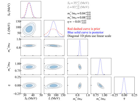
The posterior is shown in Fig. 1. Despite employing uniform priors, tight constraints on , and are observed. These constraints are robust constraints as they do not show a significant correlation with either or , indicating that their posterior values remain unaffected by our choice of prior.
In contrast, the posterior distributions of and are wide even when Gaussian priors are used. The posterior distribution of looks very similar to the prior, indicating that our choice of observables lacks sensitivity to . Although there is a modest improvement in the constraint on compared to the prior distribution, Fig. 1 also highlights a correlation between and . Consequently, the marginalized value of () may change if a different prior for is employed.
The near-zero value of indicates that the in-medium cross-section is similar to the free cross-section. This differs from previous analyses performed at different beam energies, where an enhancement in the in-medium cross-section is derived [45].
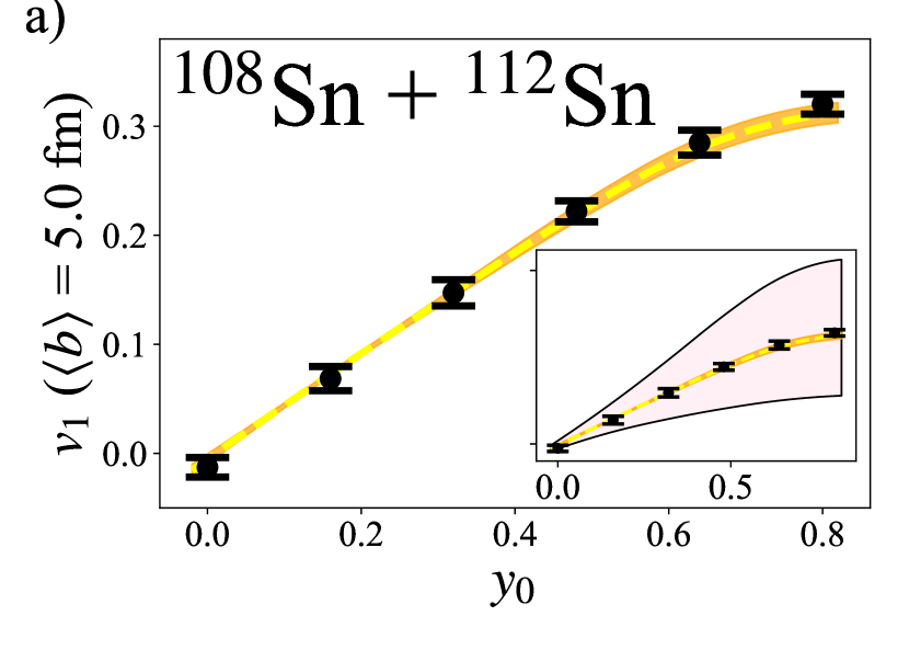
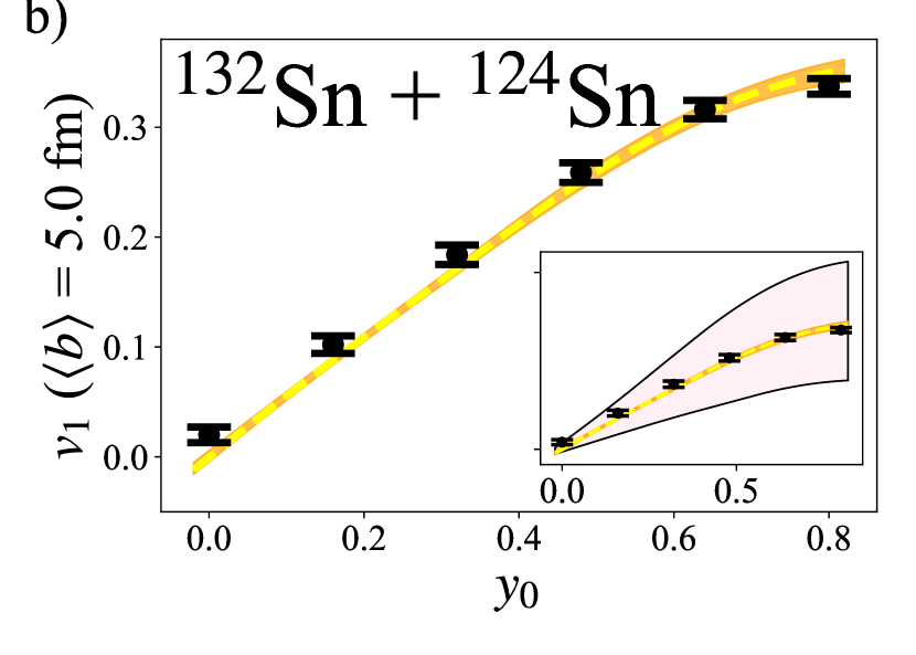
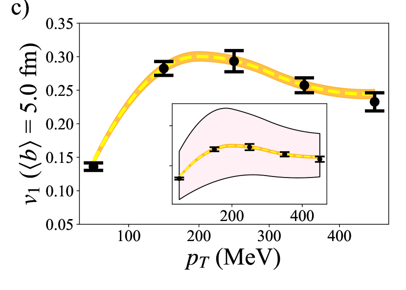
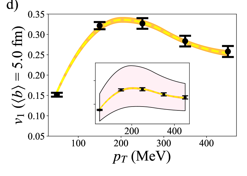
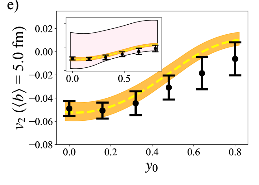
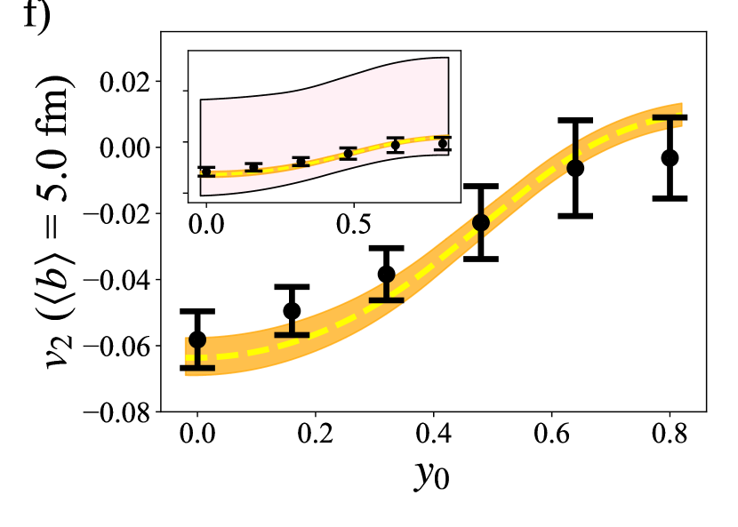
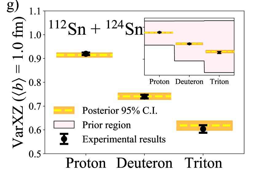
Figure 2 shows the fitted flow and stopping observables. The first three rows show the results of directed and elliptic flow, with plots on the left column corresponding to the results of 108SnSn reaction and the right 132SnSn. From top to bottom, the three rows show as a function of , as a function of (MeV) and as a function of , all at . The fourth row shows VarXZ for 112SnSn at .
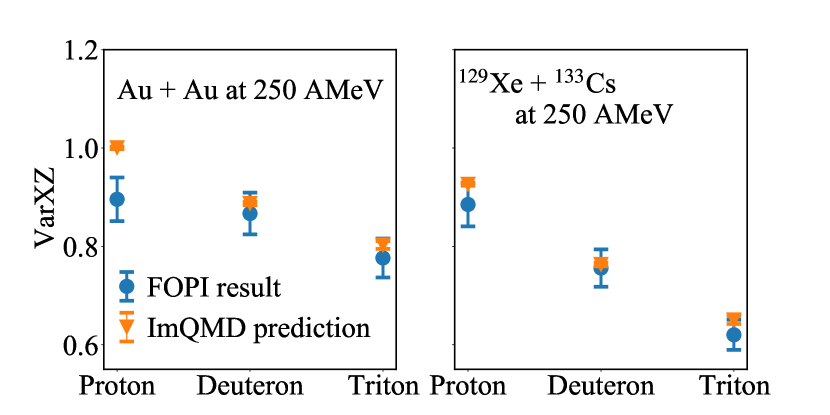
To test the prediction power of our results, our most probable values of , , , and are used to predict VarXZ of protons, deuterons and tritons for 197Au + 197Au and 129Xe + 133Cs at a fixed-target beam energy of with the ImQMD-Sky model. VarXZs from these two systems are chosen because their values were measured experimentally in Ref. [47]. Experimental values of VarXZs at other beam energies are also available, but the beam energy at is the closest to the SRIT beam energy of . Our choice minimizes effects due to changing beam energy and isolates the dependence on system size. Predictions from ImQMD-Sky are plotted on top of experimental values in Fig. 3 which shows reasonable agreement with an exception of proton from Au + Au at , where less stopping is observed than the model prediction. It is a good indication that our results are applicable to collisions of various system sizes near .
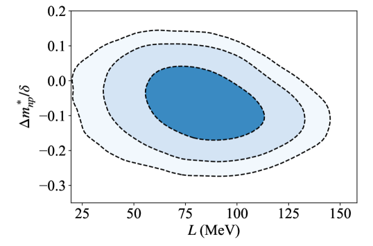
The posterior on effective masses can be converted to a probability distribution on effective mass splitting using Eq. (3) and we find that . The value of effective mass splitting differs among various analyses using different data, but most of them favor a positive value [61]. Of all the analyses in Ref. [61], the only result that favors a negative value of comes from the study of the n/p ratio from heavy ion reactions which yields [14]. That analysis also uses the ImQMD-Sky model for inference. It may indicates that the momentum dependence of the isovector mean fields in the ImQMD-Sky transport theory prefers a lower value of effective mass splitting.
Similar to constraints from pion observables [15], we observed a correlation from this analysis between and , as Fig. 4 demonstrates. The correlation trends in Ref. [15] are nearly orthogonal to the present work. While ImQMD-Sky is used for the current constraint, dcQMD was used in the pion analysis. Clearly, the model dependence of effective mass and symmetry energy effects must be studied carefully, ideally within an effort like the Transport Model Evaluation Project (TMEP) [62]. Such endeavors will deepen our understanding of model dependence of EoS parameters and hopefully develop ways for constraints from different models to be compared and combined reliably. Even though a direct comparison is not feasible right now, this study opens an opportunity to improve constraints on by combining Fig. 4 with correlated constraints between and from Ref. [15].
6 Summary and conclusion
Directed flow () and elliptic flow () of 108SnSn and 132SnSn and stopping (VarXZ) of 112SnSn (all at fixed-target beam energy of ) are extracted from the data obtained in the SRIT experiment. The measured values are compared to predictions from the Improved Quantum Molecular Dynamic-Skyrme (ImQMD-Sky) model through a Bayesian analysis which shows strong constraining power on the effective masses ( and ) and the in-medium cross-section parameter (). The most probable values are , , and . The constraints on effective mass are converted to a probability distribution on effective mass splitting to give . This can be used to tighten constraints on symmetry energy terms such as as it was demonstrated to be correlated to , but efforts in understanding model dependence of analysis on nucleon effective masses are warranted for the comparison to be conclusive.
7 Acknowledgement
The authors would like to thank members of the Transport Model Evaluation Project collaboration for many fruitful discussions. This work was supported by U.S. National Science Foundation Grant No. PHY-2209145, Department of Energy Grant No. DE-FG02-93ER40773, Department of Energy National Nuclear Security Administration Stewardship Science Graduate Fellowship under cooperative Agreement No. DE-NA0002135, the Robert A. Welch Foundation (A-1266 and A-1358), the Japanese MEXT, Japan KAKENHI (Grant-in-Aid for Scientific Research on Innovative Areas) grant No. 24105004, JSPS KAKENHI Grants Nos. JP17K05432, JP19K14709 and JP21K03528, the National Research Foundation of Korea under grant Nos. 2018R1A5A1025563 and 2013M7A1A1075764, the Polish National Science Center (NCN) under contract Nos. UMO-2013/09/B/ST2/04064, UMO-2013/-10/M/ST2/00624, the Ministry of Science and Technology of China under grant Nos. 2022YFE0103400 and Tsinghua University Initiative Scientific Research Program, Computing resources were provided by FRIB, the HOKUSAI-Great Wave system at RI-KEN, and the Institute for Cyber-Enabled Research at Michigan State University.
Appendix A SRIT data
All experimental data and uncertainties are tabulated in Table A.1.
| 0.000 | 0.160 | 0.320 | 0.480 | 0.640 | 0.800 | |
|---|---|---|---|---|---|---|
| -0.013 | 0.069 | 0.147 | 0.222 | 0.285 | 0.320 | |
| Stat. | 0.002 | 0.002 | 0.002 | 0.002 | 0.002 | 0.002 |
| Sys. | 0.009 | 0.011 | 0.012 | 0.009 | 0.011 | 0.009 |
| 0.000 | 0.160 | 0.320 | 0.480 | 0.640 | 0.800 | |
|---|---|---|---|---|---|---|
| 0.020 | 0.102 | 0.184 | 0.259 | 0.316 | 0.337 | |
| Stat | 0.002 | 0.002 | 0.002 | 0.002 | 0.002 | 0.002 |
| Sys | 0.007 | 0.008 | 0.009 | 0.009 | 0.008 | 0.007 |
| 50 | 150 | 250 | 350 | 450 | |
|---|---|---|---|---|---|
| 0.136 | 0.283 | 0.293 | 0.257 | 0.233 | |
| Stat. | 0.002 | 0.002 | 0.002 | 0.003 | 0.004 |
| Sys. | 0.005 | 0.010 | 0.016 | 0.011 | 0.013 |
| 50 | 150 | 250 | 350 | 450 | |
|---|---|---|---|---|---|
| 0.152 | 0.322 | 0.327 | 0.284 | 0.258 | |
| Stat | 0.002 | 0.002 | 0.002 | 0.003 | 0.004 |
| Sys | 0.004 | 0.009 | 0.013 | 0.013 | 0.013 |
| 0.000 | 0.160 | 0.320 | 0.480 | 0.640 | 0.800 | |
|---|---|---|---|---|---|---|
| -0.049 | -0.051 | -0.044 | -0.031 | -0.019 | -0.006 | |
| Stat. | 0.003 | 0.003 | 0.003 | 0.003 | 0.003 | 0.003 |
| Sys. | 0.006 | 0.006 | 0.010 | 0.010 | 0.013 | 0.014 |
| 0.000 | 0.160 | 0.320 | 0.480 | 0.640 | 0.800 | |
|---|---|---|---|---|---|---|
| -0.058 | -0.049 | -0.038 | -0.023 | -0.006 | -0.003 | |
| Stat. | 0.003 | 0.003 | 0.003 | 0.003 | 0.003 | 0.003 |
| Sys. | 0.008 | 0.007 | 0.007 | 0.011 | 0.014 | 0.012 |
| proton | deuteron | triton | |
|---|---|---|---|
| VarXZ | 0.915 | 0.767 | 0.590 |
| Stat. | 0.004 | 0.005 | 0.003 |
| Sys. | 0.011 | 0.012 | 0.010 |
References
-
[1]
J. Xu,
Transport
approaches for the description of intermediate-energy heavy-ion collisions,
Progress in Particle and Nuclear Physics 106 (2019) 312–359.
doi:https://doi.org/10.1016/j.ppnp.2019.02.009.
URL https://www.sciencedirect.com/science/article/pii/S0146641019300213 - [2] A. Sorensen, K. Agarwal, K. W. Brown, Z. Chajecki, P. Danielewicz, C. Drischler, S. Gandolfi, J. W. Holt, M. Kaminski, C.-M. Ko, R. Kumar, B.-A. Li, W. G. Lynch, A. B. McIntosh, W. G. Newton, S. Pratt, O. Savchuk, M. Stefaniak, I. Tews, M. B. Tsang, R. Vogt, H. Wolter, H. Zbroszczyk, N. Abbasi, J. Aichelin, A. Andronic, S. A. Bass, F. Becattini, D. Blaschke, M. Bleicher, C. Blume, E. Bratkovskaya, B. A. Brown, D. A. Brown, A. Camaiani, G. Casini, K. Chatziioannou, A. Chbihi, M. Colonna, M. D. Cozma, V. Dexheimer, X. Dong, T. Dore, L. Du, J. A. Dueñas, H. Elfner, W. Florkowski, Y. Fujimoto, R. J. Furnstahl, A. Gade, T. Galatyuk, C. Gale, F. Geurts, S. Grozdanov, K. Hagel, S. P. Harris, W. Haxton, U. Heinz, M. P. Heller, O. Hen, H. Hergert, N. Herrmann, H. Z. Huang, X.-G. Huang, N. Ikeno, G. Inghirami, J. Jankowski, J. Jia, J. C. Jiménez, J. Kapusta, B. Kardan, I. Karpenko, D. Keane, D. Kharzeev, A. Kugler, A. L. Fèvre, D. Lee, H. Liu, M. A. Lisa, W. J. Llope, I. Lombardo, M. Lorenz, T. Marchi, L. McLerran, U. Mosel, A. Motornenko, B. Müller, P. Napolitani, J. B. Natowitz, W. Nazarewicz, J. Noronha, J. Noronha-Hostler, G. Odyniec, P. Papakonstantinou, Z. Paulínyová, J. Piekarewicz, R. D. Pisarski, C. Plumberg, M. Prakash, J. Randrup, C. Ratti, P. Rau, S. Reddy, H.-R. Schmidt, P. Russotto, R. Ryblewski, A. Schäfer, B. Schenke, S. Sen, P. Senger, R. Seto, C. Shen, B. Sherrill, M. Singh, V. Skokov, M. Spaliński, J. Steinheimer, M. Stephanov, J. Stroth, C. Sturm, K.-J. Sun, A. Tang, G. Torrieri, W. Trautmann, G. Verde, V. Vovchenko, R. Wada, F. Wang, G. Wang, K. Werner, N. Xu, Z. Xu, H.-U. Yee, S. Yennello, Y. Yin, Dense nuclear matter equation of state from heavy-ion collisions (2023). arXiv:2301.13253.
-
[3]
W. Lynch, M. Tsang,
Decoding
the density dependence of the nuclear symmetry energy, Physics Letters B 830
(2022) 137098.
doi:https://doi.org/10.1016/j.physletb.2022.137098.
URL https://www.sciencedirect.com/science/article/pii/S0370269322002325 - [4] P. Danielewicz, R. Lacey, W. G. Lynch, Determination of the Equation of State of Dense Matter, Science 298 (5598) (2002) 1592–1596. doi:10.1126/science.1078070.
-
[5]
A. L. Fèvre, Y. Leifels, W. Reisdorf, J. Aichelin, C. Hartnack,
Constraining
the nuclear matter equation of state around twice saturation density,
Nuclear Physics A 945 (2016) 112 – 133.
doi:https://doi.org/10.1016/j.nuclphysa.2015.09.015.
URL http://www.sciencedirect.com/science/article/pii/S0375947415002225 -
[6]
M. Dutra, O. Lourenço, J. S. Sá Martins,
A. Delfino, J. R. Stone, P. D. Stevenson,
Skyrme
interaction and nuclear matter constraints, Phys. Rev. C 85 (2012)
035201.
doi:10.1103/PhysRevC.85.035201.
URL https://link.aps.org/doi/10.1103/PhysRevC.85.035201 - [7] Z. Zhang, L.-W. Chen, Electric dipole polarizability in 208Pb as a probe of the symmetry energy and neutron matter around , Physical Review C 92 (3) (2015) 031301.
-
[8]
D. Adhikari, H. Albataineh, D. Androic, K. Aniol, D. S. Armstrong, T. Averett,
C. Ayerbe Gayoso, S. Barcus, V. Bellini, R. S. Beminiwattha, J. F. Benesch,
H. Bhatt, D. Bhatta Pathak, D. Bhetuwal, B. Blaikie, Q. Campagna,
A. Camsonne, G. D. Cates, Y. Chen, C. Clarke, J. C. Cornejo, S. Covrig Dusa,
P. Datta, A. Deshpande, D. Dutta, C. Feldman, E. Fuchey, C. Gal, D. Gaskell,
T. Gautam, M. Gericke, C. Ghosh, I. Halilovic, J.-O. Hansen, F. Hauenstein,
W. Henry, C. J. Horowitz, C. Jantzi, S. Jian, S. Johnston, D. C. Jones,
B. Karki, S. Katugampola, C. Keppel, P. M. King, D. E. King, M. Knauss, K. S.
Kumar, T. Kutz, N. Lashley-Colthirst, G. Leverick, H. Liu, N. Liyange,
S. Malace, R. Mammei, J. Mammei, M. McCaughan, D. McNulty, D. Meekins,
C. Metts, R. Michaels, M. M. Mondal, J. Napolitano, A. Narayan, D. Nikolaev,
M. N. H. Rashad, V. Owen, C. Palatchi, J. Pan, B. Pandey, S. Park, K. D.
Paschke, M. Petrusky, M. L. Pitt, S. Premathilake, A. J. R. Puckett,
B. Quinn, R. Radloff, S. Rahman, A. Rathnayake, B. T. Reed, P. E. Reimer,
R. Richards, S. Riordan, Y. Roblin, S. Seeds, A. Shahinyan, P. Souder,
L. Tang, M. Thiel, Y. Tian, G. M. Urciuoli, E. W. Wertz, B. Wojtsekhowski,
B. Yale, T. Ye, A. Yoon, A. Zec, W. Zhang, J. Zhang, X. Zheng,
Accurate
Determination of the Neutron Skin Thickness of
through Parity-Violation in Electron Scattering, Phys. Rev.
Lett. 126 (2021) 172502.
doi:10.1103/PhysRevLett.126.172502.
URL https://link.aps.org/doi/10.1103/PhysRevLett.126.172502 - [9] B. T. Reed, F. J. Fattoyev, C. J. Horowitz, J. Piekarewicz, Implications of PREX-2 on the Equation of State of Neutron-Rich Matter, Physical Review Letters 126 (17) (2021) 172503.
-
[10]
B. A. Brown,
Constraints
on the Skyrme Equations of State from Properties of Doubly Magic
Nuclei, Phys. Rev. Lett. 111 (2013) 232502.
doi:10.1103/PhysRevLett.111.232502.
URL https://link.aps.org/doi/10.1103/PhysRevLett.111.232502 - [11] M. Kortelainen, J. McDonnell, W. Nazarewicz, P.-G. Reinhard, J. Sarich, N. Schunck, M. V. Stoitsov, S. M. Wild, Nuclear energy density optimization: Large deformations, Physical Review C 85 (2) (2012) 024304.
- [12] P. Danielewicz, P. Singh, J. Lee, Symmetry Energy III: Isovector Skins, Nucl. Phys. A958 (2017) 147–186. arXiv:1611.01871, doi:10.1016/j.nuclphysa.2016.11.008.
-
[13]
M. B. Tsang, Y. Zhang, P. Danielewicz, M. Famiano, Z. Li, W. G. Lynch, A. W.
Steiner,
Constraints
on the Density Dependence of the Symmetry Energy, Phys. Rev.
Lett. 102 (2009) 122701.
doi:10.1103/PhysRevLett.102.122701.
URL https://link.aps.org/doi/10.1103/PhysRevLett.102.122701 -
[14]
P. Morfouace, C. Tsang, Y. Zhang, W. Lynch, M. Tsang, D. Coupland, M. Youngs,
Z. Chajecki, M. Famiano, T. Ghosh, G. Jhang, J. Lee, H. Liu, A. Sanetullaev,
R. Showalter, J. Winkelbauer,
Constraining
the symmetry energy with heavy-ion collisions and Bayesian analyses,
Physics Letters B 799 (2019) 135045.
doi:https://doi.org/10.1016/j.physletb.2019.135045.
URL https://www.sciencedirect.com/science/article/pii/S0370269319307671 -
[15]
J. Estee, W. G. Lynch, C. Y. Tsang, J. Barney, G. Jhang, M. B. Tsang, R. Wang,
M. Kaneko, J. W. Lee, T. Isobe, M. Kurata-Nishimura, T. Murakami, D. S. Ahn,
L. Atar, T. Aumann, H. Baba, K. Boretzky, J. Brzychczyk, G. Cerizza,
N. Chiga, N. Fukuda, I. Gasparic, B. Hong, A. Horvat, K. Ieki, N. Inabe,
Y. J. Kim, T. Kobayashi, Y. Kondo, P. Lasko, H. S. Lee, Y. Leifels,
J. Łukasik, J. Manfredi, A. B. McIntosh, P. Morfouace, T. Nakamura,
N. Nakatsuka, S. Nishimura, H. Otsu, P. Pawłowski, K. Pelczar, D. Rossi,
H. Sakurai, C. Santamaria, H. Sato, H. Scheit, R. Shane, Y. Shimizu,
H. Simon, A. Snoch, A. Sochocka, T. Sumikama, H. Suzuki, D. Suzuki,
H. Takeda, S. Tangwancharoen, H. Toernqvist, Y. Togano, Z. G. Xiao, S. J.
Yennello, Y. Zhang, M. D. Cozma,
Probing the
Symmetry Energy with the Spectral Pion Ratio, Phys. Rev.
Lett. 126 (2021) 162701.
doi:10.1103/PhysRevLett.126.162701.
URL https://link.aps.org/doi/10.1103/PhysRevLett.126.162701 - [16] M. Cozma, Feasibility of constraining the curvature parameter of the symmetry energy using elliptic flow data, The European Physical Journal A 54 (3) (2018) 1–23.
-
[17]
P. Russotto, P. Wu, M. Zoric, M. Chartier, Y. Leifels, R. Lemmon, Q. Li,
J. Łukasik, A. Pagano, P. Pawłowski, W. Trautmann,
Symmetry
energy from elliptic flow in 197au+197au, Physics Letters B 697 (5) (2011)
471–476.
doi:https://doi.org/10.1016/j.physletb.2011.02.033.
URL https://www.sciencedirect.com/science/article/pii/S037026931100178X -
[18]
P. Russotto, et al.,
Results of the
ASY-EOS experiment at GSI: The symmetry energy at
suprasaturation density, Phys. Rev. C 94 (2016) 034608.
doi:10.1103/PhysRevC.94.034608.
URL https://link.aps.org/doi/10.1103/PhysRevC.94.034608 -
[19]
J. Margueron, R. Hoffmann Casali, F. Gulminelli,
Equation of
state for dense nucleonic matter from metamodeling. I. Foundational
aspects, Phys. Rev. C 97 (2018) 025805.
doi:10.1103/PhysRevC.97.025805.
URL https://link.aps.org/doi/10.1103/PhysRevC.97.025805 -
[20]
Y. Zhang, M. Liu, C.-J. Xia, Z. Li, S. K. Biswal,
Constraints on
the symmetry energy and its associated parameters from nuclei to neutron
stars, Phys. Rev. C 101 (2020) 034303.
doi:10.1103/PhysRevC.101.034303.
URL https://link.aps.org/doi/10.1103/PhysRevC.101.034303 -
[21]
B.-A. Li,
Constraining the
neutron-proton effective mass splitting in neutron-rich matter, Phys.
Rev. C 69 (2004) 064602.
doi:10.1103/PhysRevC.69.064602.
URL https://link.aps.org/doi/10.1103/PhysRevC.69.064602 -
[22]
K. Brueckner,
Two-body
forces and nuclear saturation. III. Details of the structure of the
nucleus, Physical Review 97 (5) (1955) 1353–1366, cited By 388.
doi:10.1103/PhysRev.97.1353.
URL https://www.scopus.com/inward/record.uri?eid=2-s2.0-36149019045&doi=10.1103%2fPhysRev.97.1353&partnerID=40&md5=e718dea1d3cc1243be7b9ecff14acd94 -
[23]
C. Mahaux, P. Bortignon, R. Broglia, C. Dasso,
Dynamics
of the shell model, Physics Reports 120 (1) (1985) 1–274.
doi:https://doi.org/10.1016/0370-1573(85)90100-0.
URL https://www.sciencedirect.com/science/article/pii/0370157385901000 - [24] P. Ring, P. Schuck, The nuclear many-body problem, Springer-Verlag, New York, 1980.
- [25] B.-A. Li, B.-J. Cai, L.-W. Chen, J. Xu, Nucleon effective masses in neutron-rich matter, Progress in Particle and Nuclear Physics 99 (2018) 29–119.
- [26] J. E. Barney, Charged Pion Emission from 112Sn + 124Sn and 124Sn + 112Sn Reactions with the SRIT Time Projection Chamber, Ph.D. thesis.
-
[27]
R. Shane, A. B. McIntosh, T. Isobe, W. G. Lynch, H. Baba, J. Barney,
Z. Chajecki, M. Chartier, J. Estee, M. Famiano, B. Hong, K. Ieki, G. Jhang,
R. Lemmon, F. Lu, T. Murakami, N. Nakatsuka, M. Nishimura, R. Olsen,
W. Powell, H. Sakurai, A. Taketani, S. Tangwancharoen, M. B. Tsang,
T. Usukura, R. Wang, S. J. Yennello, J. Yurkon,
Srit:
A time-projection chamber for symmetry-energy studies, Nuclear Instruments
and Methods in Physics Research Section A: Accelerators, Spectrometers,
Detectors and Associated Equipment 784 (2015) 513 – 517, Symposium on
Radiation Measurements and Applications 2014 (SORMA XV).
doi:https://doi.org/10.1016/j.nima.2015.01.026.
URL http://www.sciencedirect.com/science/article/pii/S0168900215000534 -
[28]
J. Estee, W. Lynch, J. Barney, G. Cerizza, G. Jhang, J. Lee, R. Wang, T. Isobe,
M. Kaneko, M. Kurata-Nishimura, T. Murakami, R. Shane, S. Tangwancharoen,
C. Tsang, M. Tsang, B. Hong, P. Lasko, J. Łukasik, A. McIntosh,
P. Pawłowski, K. Pelczar, H. Sakurai, C. Santamaria, D. Suzuki, S. Yennello,
Y. Zhang,
Extending
the dynamic range of electronics in a Time Projection Chamber,
Nuclear Instruments and Methods in Physics Research Section A:
Accelerators, Spectrometers, Detectors and Associated Equipment 944
(2019) 162509.
doi:https://doi.org/10.1016/j.nima.2019.162509.
URL https://www.sciencedirect.com/science/article/pii/S0168900219310472 -
[29]
J. Lee, G. Jhang, G. Cerizza, J. Barney, J. Estee, T. Isobe, M. Kaneko,
M. Kurata-Nishimura, W. Lynch, T. Murakami, C. Tsang, M. Tsang, R. Wang,
B. Hong, A. McIntosh, H. Sakurai, C. Santamaria, R. Shane, S. Tangwancharoen,
S. Yennello, Y. Zhang,
Charged
particle track reconstruction with SRIT Time Projection
Chamber, Nuclear Instruments and Methods in Physics Research
Section A: Accelerators, Spectrometers, Detectors and Associated
Equipment 965 (2020) 163840.
doi:https://doi.org/10.1016/j.nima.2020.163840.
URL https://www.sciencedirect.com/science/article/pii/S0168900220303545 -
[30]
G. Jhang, J. Estee, J. Barney, G. Cerizza, M. Kaneko, J. Lee, W. Lynch,
T. Isobe, M. Kurata-Nishimura, T. Murakami, C. Tsang, M. Tsang, R. Wang,
D. Ahn, L. Atar, T. Aumann, H. Baba, K. Boretzky, J. Brzychczyk, N. Chiga,
N. Fukuda, I. Gasparic, B. Hong, A. Horvat, K. Ieki, N. Inabe, Y. Kim,
T. Kobayashi, Y. Kondo, P. Lasko, H. Lee, Y. Leifels, J. Łukasik,
J. Manfredi, A. McIntosh, P. Morfouace, T. Nakamura, N. Nakatsuka,
S. Nishimura, R. Olsen, H. Otsu, P. Pawłowski, K. Pelczar, D. Rossi,
H. Sakurai, C. Santamaria, H. Sato, H. Scheit, R. Shane, Y. Shimizu,
H. Simon, A. Snoch, A. Sochocka, Z. Sosin, T. Sumikama, H. Suzuki, D. Suzuki,
H. Takeda, S. Tangwancharoen, H. Toernqvist, Y. Togano, Z. Xiao, S. Yennello,
J. Yurkon, Y. Zhang, M. Colonna, D. Cozma, P. Danielewicz, H. Elfner,
N. Ikeno, C. M. Ko, J. Mohs, D. Oliinychenko, A. Ono, J. Su, Y. J. Wang,
H. Wolter, J. Xu, Y.-X. Zhang, Z. Zhang,
Symmetry
energy investigation with pion production from Sn+Sn systems, Physics
Letters B 813 (2021) 136016.
doi:https://doi.org/10.1016/j.physletb.2020.136016.
URL https://www.sciencedirect.com/science/article/pii/S0370269320308194 - [31] M. Kaneko, Hydrogen Isotope Productions in Sn + Sn Collisions with Radioactive Beams at 270 MeV/nucleon, Ph.D. thesis, Kyoto University (2022).
-
[32]
J. W. Lee, M. B. Tsang, C. Y. Tsang, R. Wang, J. Barney, J. Estee, T. Isobe,
M. Kaneko, M. Kurata-Nishimura, W. G. Lynch, T. Murakami, A. Ono, S. R.
Souza, D. S. Ahn, L. Atar, T. Aumann, H. Baba, K. Boretzky, J. Brzychczyk,
G. Cerizza, N. Chiga, N. Fukuda, I. Gasparic, B. Hong, A. Horvat, K. Ieki,
N. Ikeno, N. Inabe, G. Jhang, Y. J. Kim, T. Kobayashi, Y. Kondo, P. Lasko,
H. S. Lee, Y. Leifels, J. Łukasik, J. Manfredi, A. B. McIntosh,
P. Morfouace, T. Nakamura, N. Nakatsuka, S. Nishimura, H. Otsu,
P. Pawłowski, K. Pelczar, D. Rossi, H. Sakurai, C. Santamaria, H. Sato,
H. Scheit, R. Shane, Y. Shimizu, H. Simon, A. Snoch, A. Sochocka,
T. Sumikama, H. Suzuki, D. Suzuki, H. Takeda, S. Tangwancharoen, Y. Togano,
Z. G. Xiao, S. J. Yennello, Y. Zhang, t. S. p. R. collaboration),
Isoscaling in central
Sn+Sn collisions at 270 MeV/u, The European Physical Journal A 58 (10)
(2022) 201.
doi:10.1140/epja/s10050-022-00851-2.
URL https://doi.org/10.1140/epja/s10050-022-00851-2 -
[33]
F. Rami, P. Crochet, R. Donà, B. de Schauenburg, P. Wagner, J. Alard,
A. Andronic, Z. Basrak, N. Bastid, I. Belyaev, A. Bendarag, G. Berek,
D. Best, R. Čaplar, A. Devismes, P. Dupieux, M. Dželalija, M. Eskef,
Z. Fodor, A. Gobbi, Y. Grishkin, N. Herrmann, K. Hildenbrand, B. Hong,
J. Kecskemeti, M. Kirejczyk, M. Korolija, R. Kotte, A. Lebedev, Y. Leifels,
H. Merlitz, S. Mohren, D. Moisa, W. Neubert, D. Pelte, M. Petrovici,
C. Pinkenburg, C. Plettner, W. Reisdorf, D. Schüll, Z. Seres, B. Sikora,
V. Simion, K. Siwek-Wilczyńska, G. Stoicea, M. Stockmeir, M. Vasiliev,
K. Wisniewski, D. Wohlfarth, I. Yushmanov, A. Zhilin,
Flow
angle from intermediate mass fragment measurements, Nuclear Physics A
646 (3) (1999) 367–384.
doi:https://doi.org/10.1016/S0375-9474(98)00641-1.
URL https://www.sciencedirect.com/science/article/pii/S0375947498006411 -
[34]
A. Andronic, W. Reisdorf, J. P. Alard, V. Barret, Z. Basrak, N. Bastid,
A. Bendarag, G. Berek, R. Čaplar,
P. Crochet, A. Devismes, P. Dupieux, M. Dželalija, C. Finck, Z. Fodor, A. Gobbi, Y. Grishkin, O. N. Hartmann,
N. Herrmann, K. D. Hildenbrand, B. Hong, J. Kecskemeti, Y. J. Kim,
M. Kirejczyk, P. Koczon, M. Korolija, R. Kotte, T. Kress, R. Kutsche,
A. Lebedev, Y. Leifels, W. Neubert, D. Pelte, M. Petrovici, F. Rami,
B. de Schauenburg, D. Schüll, Z. Seres, B. Sikora, K. S. Sim, V. Simion,
K. Siwek-Wilczyńska, V. Smolyankin, M. R.
Stockmeier, G. Stoicea, P. Wagner, K. Wiśniewski, D. Wohlfarth, I. Yushmanov, A. Zhilin,
Differential
directed flow in Au+Au collisions, Phys. Rev. C 64 (2001) 041604.
doi:10.1103/PhysRevC.64.041604.
URL https://link.aps.org/doi/10.1103/PhysRevC.64.041604 -
[35]
De Filippo, E., Russotto, P., Acosta, L., Adamczyk, M., Al-Ajlan, A.,
Al-Garawi, M., Al-Homaidhi, S., Amorini, F., Auditore, L., Aumann,
T., Ayyad, Y., Basrak, Z., Benlliure, J., Boisjoli, M., Boretzky,
K., Brzychczyk, J., Budzanowski, A., Caesar, C., Cardella, G.,
Cammarata, P., Chajecki, Z., Chartier, M., Chbihi, A., Colonna, M.,
Cozma, M.D., Czech, B., Di Toro, M., Famiano, M., Gannon, S.,
Gaspari´c, I., Grassi, L., Guazzoni, C., Guazzoni, P., Heil, M.,
Heilborn, L., Introzzi, R., Isobe, T., Kezzar, K., Kis, M.,
Krasznahorkay, A., Kupny, S., Kurz, N., La Guidara, E., Lanzalone,
G., Lasko, P., Le Fèvre, A., Leifels, Y., Lemmon, R.C., Li,
Q.F., Lombardo, I., Lukasik, J., Lynch, W.G., Marini, P., Matthews,
Z., May, L., Minniti, T., Mostazo, M., Pagano, A., Pagano, E.V.,
Papa, M., Pawlowski, P., Pirrone, S., Politi, G., Porto, F.,
Reviol, W., Riccio, F., Rizzo, F., Rosato, E., Rossi, D., Santoro,
S., Sarantites, D.G., Simon, H., Skwirczynska, I., Sosin, Z.,
Stuhl, L., Trautmann, W., Trifirò, A., Trimarchi, M., Tsang,
M.B., Verde, G., Veselsky, M., Vigilante, M., Wang, Yongjia,
Wieloch, A., Wigg, P., Winkelbauer, J., Wolter, H.H., Wu, P.,
Yennello, S., Zambon, P., Zetta, L., Zoric, M.,
The symmetry energy at
suprasaturation density and the ASY-EOS experiment at GSI,
EPJ Web Conf. 137 (2017) 09002.
doi:10.1051/epjconf/201713709002.
URL https://doi.org/10.1051/epjconf/201713709002 - [36] A. Le Fevre, Y. Leifels, W. Reisdorf, J. Aichelin, C. Hartnack, Constraining the nuclear matter equation of state around twice saturation density, Nuclear Physics A 945 (2016) 112–133.
-
[37]
P. Russotto, M. D. Cozma, E. D. Filippo, A. L. Fèvre, Y. Leifels,
J. Łukasik, Studies
of the equation-of-state of nuclear matter by heavy-ion collisions at
intermediate energy in the multi-messenger era, La Rivista del Nuovo Cimento
46 (1) (2023) 1–70.
doi:10.1007/s40766-023-00039-4.
URL https://doi.org/10.1007%2Fs40766-023-00039-4 -
[38]
G. Stoicea, M. Petrovici, A. Andronic, N. Herrmann, J. P. Alard, Z. Basrak,
V. Barret, N. Bastid, R. Čaplar, P. Crochet,
P. Dupieux, M. Dželalija, Z. Fodor,
O. Hartmann, K. D. Hildenbrand, B. Hong, J. Kecskemeti, Y. J. Kim,
M. Kirejczyk, M. Korolija, R. Kotte, T. Kress, A. Lebedev, Y. Leifels,
X. Lopez, M. Merschmeier, W. Neubert, D. Pelte, F. Rami, W. Reisdorf,
D. Schüll, Z. Seres, B. Sikora, K. S. Sim, V. Simion,
K. Siwek-Wilczyńska, V. Smolyankin,
M. Stockmeier, K. Wiśniewski, D. Wohlfarth,
I. Yushmanov, A. Zhilin, P. Danielewicz,
Azimuthal
dependence of collective expansion for symmetric heavy-ion collisions, Phys.
Rev. Lett. 92 (2004) 072303.
doi:10.1103/PhysRevLett.92.072303.
URL https://link.aps.org/doi/10.1103/PhysRevLett.92.072303 -
[39]
W. Reisdorf, Y. Leifels, A. Andronic, R. Averbeck, V. Barret, Z. Basrak,
N. Bastid, M. Benabderrahmane, R. Čaplar, P. Crochet, P. Dupieux,
M. Dželalija, Z. Fodor, P. Gasik, Y. Grishkin, O. Hartmann, N. Herrmann,
K. Hildenbrand, B. Hong, T. Kang, J. Kecskemeti, Y. Kim, M. Kirejczyk,
M. Kiš, P. Koczoń, M. Korolija, R. Kotte, T. Kress, A. Lebedev, X. Lopez,
T. Matulewicz, M. Merschmeyer, W. Neubert, M. Petrovici, K. Piasecki,
F. Rami, M. Ryu, A. Schüttauf, Z. Seres, B. Sikora, K. Sim, V. Simion,
K. Siwek-Wilczyńska, V. Smolyankin, M. Stockmeier, G. Stoicea, Z. Tymiński,
K. Wiśniewski, D. Wohlfarth, Z. Xiao, H. Xu, I. Yushmanov, A. Zhilin,
Systematics
of azimuthal asymmetries in heavy ion collisions in the 1a gev regime,
Nuclear Physics A 876 (2012) 1–60.
doi:https://doi.org/10.1016/j.nuclphysa.2011.12.006.
URL https://www.sciencedirect.com/science/article/pii/S0375947411006877 -
[40]
S. Voloshin, Y. Zhang, Flow study
in relativistic nuclear collisions by fourier expansion of azimuthal particle
distributions, Zeitschrift für Physik C Particles and Fields 70 (4)
(1996) 665–671.
doi:10.1007/s002880050141.
URL https://doi.org/10.1007/s002880050141 -
[41]
A. M. Poskanzer, S. A. Voloshin,
Methods for
analyzing anisotropic flow in relativistic nuclear collisions, Phys.
Rev. C 58 (1998) 1671–1678.
doi:10.1103/PhysRevC.58.1671.
URL https://link.aps.org/doi/10.1103/PhysRevC.58.1671 -
[42]
A. Ono,
Dynamics
of clusters and fragments in heavy-ion collisions, Progress in Particle
and Nuclear Physics 105 (2019) 139–179.
doi:https://doi.org/10.1016/j.ppnp.2018.11.001.
URL https://www.sciencedirect.com/science/article/pii/S0146641018300863 -
[43]
B. Dönigus,
Selected highlights
of the production of light (anti-)(hyper-)nuclei in ultra-relativistic
heavy-ion collisions, The European Physical Journal A 56 (11)
(2020) 280.
doi:10.1140/epja/s10050-020-00275-w.
URL https://doi.org/10.1140/epja/s10050-020-00275-w -
[44]
P. Gossiaux, R. Puri, C. Hartnack, J. Aichelin,
The
multifragmentation of spectator matter, Nuclear Physics A 619 (3) (1997)
379–390.
doi:https://doi.org/10.1016/S0375-9474(97)00175-9.
URL https://www.sciencedirect.com/science/article/pii/S0375947497001759 -
[45]
X. Chen, Y. Zhang, Z. li,
Theoretical uncertainties
on the extraction of in-medium NN cross sections by different Pauli
blocking algorithms, Chinese Physics C (Apr 2021).
doi:10.1088/1674-1137/abfb51.
URL https://doi.org/10.1088/1674-1137/abfb51 -
[46]
P. Li, Y. Wang, Q. Li, H. Zhang,
Accessing
the in-medium effects on nucleon-nucleon elastic cross section with
collective flows and nuclear stopping, Physics Letters B 828 (2022) 137019.
doi:https://doi.org/10.1016/j.physletb.2022.137019.
URL https://www.sciencedirect.com/science/article/pii/S0370269322001538 -
[47]
W. Reisdorf, A. Andronic, R. Averbeck, M. Benabderrahmane, O. Hartmann,
N. Herrmann, K. Hildenbrand, T. Kang, Y. Kim, M. Kiš, P. Koczoń, T. Kress,
Y. Leifels, M. Merschmeyer, K. Piasecki, A. Schüttauf, M. Stockmeier,
V. Barret, Z. Basrak, N. Bastid, R. Čaplar, P. Crochet, P. Dupieux,
M. Dželalija, Z. Fodor, P. Gasik, Y. Grishkin, B. Hong, J. Kecskemeti,
M. Kirejczyk, M. Korolija, R. Kotte, A. Lebedev, X. Lopez, T. Matulewicz,
W. Neubert, M. Petrovici, F. Rami, M. Ryu, Z. Seres, B. Sikora, K. Sim,
V. Simion, K. Siwek-Wilczyńska, V. Smolyankin, G. Stoicea, Z. Tymiński,
K. Wiśniewski, D. Wohlfarth, Z. Xiao, H. Xu, I. Yushmanov, A. Zhilin,
Systematics
of central heavy ion collisions in the 1A GeV regime, Nuclear
Physics A 848 (3) (2010) 366–427.
doi:https://doi.org/10.1016/j.nuclphysa.2010.09.008.
URL https://www.sciencedirect.com/science/article/pii/S0375947410006810 -
[48]
T. Gaitanos, C. Fuchs, H. Wolter,
Nuclear
stopping and flow in heavy-ion collisions and the in-medium NN cross
section, Physics Letters B 609 (3) (2005) 241–246.
doi:https://doi.org/10.1016/j.physletb.2005.01.069.
URL https://www.sciencedirect.com/science/article/pii/S0370269305001486 -
[49]
J. Barney, J. Estee, W. G. Lynch, T. Isobe, G. Jhang, M. Kurata-Nishimura,
A. B. McIntosh, T. Murakami, R. Shane, S. Tangwancharoen, M. B. Tsang,
G. Cerizza, M. Kaneko, J. W. Lee, C. Y. Tsang, R. Wang, C. Anderson, H. Baba,
Z. Chajecki, M. Famiano, R. Hodges-Showalter, B. Hong, T. Kobayashi,
P. Lasko, J. Łukasik, N. Nakatsuka, R. Olsen, H. Otsu, P. Pawłowski,
K. Pelczar, H. Sakurai, C. Santamaria, H. Setiawan, A. Taketani, J. R.
Winkelbauer, Z. Xiao, S. J. Yennello, J. Yurkon, Y. Zhang,
The SRIT time
projection chamber, Review of Scientific Instruments 92 (6) (6 2021).
doi:10.1063/5.0041191.
URL https://www.osti.gov/biblio/1797552 -
[50]
M. Kaneko, T. Murakami, T. Isobe, M. Kurata-Nishimura, A. Ono, N. Ikeno,
J. Barney, G. Cerizza, J. Estee, G. Jhang, J. Lee, W. Lynch, C. Santamaria,
C. Tsang, M. Tsang, R. Wang, D. Ahn, L. Atar, T. Aumann, H. Baba,
K. Boretzky, J. Brzychczyk, N. Chiga, N. Fukuda, I. Gašparić, B. Hong,
A. Horvat, T. Ichihara, K. Ieki, N. Inabe, Y. Kim, T. Kobayashi, Y. Kondo,
P. Lasko, H. Lee, Y. Leifels, J. Łukasik, J. Manfredi, A. McIntosh,
P. Morfouace, T. Nakamura, N. Nakatsuka, S. Nishimura, R. Olsen, H. Otsu,
P. Pawłowski, K. Pelczar, D. Rossi, H. Sakurai, H. Sato, H. Scheit,
R. Shane, Y. Shimizu, H. Simon, T. Sumikama, D. Suzuki, H. Suzuki, H. Takeda,
S. Tangwancharoen, Y. Togano, H. Törnqvist, Z. Xiao, S. Yennello, J. Yurkon,
Y. Zhang,
Rapidity
distributions of Z = 1 isotopes and the nuclear symmetry energy from
Sn+Sn collisions with radioactive beams at 270 MeV/nucleon,
Physics Letters B 822 (2021) 136681.
doi:https://doi.org/10.1016/j.physletb.2021.136681.
URL https://www.sciencedirect.com/science/article/pii/S0370269321006213 -
[51]
Y. Zhang, M. Tsang, Z. Li, H. Liu,
Constraints
on nucleon effective mass splitting with heavy ion collisions, Phys.
Lett. B 732 (2014) 186–190.
doi:https://doi.org/10.1016/j.physletb.2014.03.030.
URL https://www.sciencedirect.com/science/article/pii/S0370269314001865 -
[52]
Y. Zhang, M. Tsang, Z. Li,
Covariance
analysis of symmetry energy observables from heavy ion collision, Physics
Letters B 749 (2015) 262–266.
doi:https://doi.org/10.1016/j.physletb.2015.07.064.
URL https://www.sciencedirect.com/science/article/pii/S0370269315005742 -
[53]
T. H. R. Skyrme, Cvii. the
nuclear surface, The Philosophical Magazine: A Journal of Theoretical
Experimental and Applied Physics 1 (11) (1956) 1043–1054.
arXiv:https://doi.org/10.1080/14786435608238186, doi:10.1080/14786435608238186.
URL https://doi.org/10.1080/14786435608238186 -
[54]
D. Vautherin, D. M. Brink,
Hartree-fock
calculations with skyrme’s interaction. i. spherical nuclei, Phys. Rev. C 5
(1972) 626–647.
doi:10.1103/PhysRevC.5.626.
URL https://link.aps.org/doi/10.1103/PhysRevC.5.626 -
[55]
E. Chabanat, P. Bonche, P. Haensel, J. Meyer, R. Schaeffer,
A
skyrme parametrization from subnuclear to neutron star densities, Nuclear
Physics A 627 (4) (1997) 710–746.
doi:https://doi.org/10.1016/S0375-9474(97)00596-4.
URL https://www.sciencedirect.com/science/article/pii/S0375947497005964 -
[56]
B. K. Agrawal, S. Shlomo, V. K. Au,
Determination of
the parameters of a skyrme type effective interaction using the simulated
annealing approach, Phys. Rev. C 72 (2005) 014310.
doi:10.1103/PhysRevC.72.014310.
URL https://link.aps.org/doi/10.1103/PhysRevC.72.014310 -
[57]
L.-W. Chen, B.-J. Cai, C. M. Ko, B.-A. Li, C. Shen, J. Xu,
Higher-order
effects on the incompressibility of isospin asymmetric nuclear matter, Phys.
Rev. C 80 (2009) 014322.
doi:10.1103/PhysRevC.80.014322.
URL https://link.aps.org/doi/10.1103/PhysRevC.80.014322 -
[58]
J. Cugnon, D. L’Hôte, J. Vandermeulen,
Simple
parametrization of cross-sections for nuclear transport studies up to the
GeV range, Nuclear Instruments and Methods in Physics
Research, Section B: Beam Interactions with Materials and Atoms
111 (3-4) (1996) 215–220, cited By 95.
doi:10.1016/0168-583X(95)01384-9.
URL https://www.scopus.com/inward/record.uri?eid=2-s2.0-0030143153&doi=10.1016%2f0168-583X%2895%2901384-9&partnerID=40&md5=e6854ad674cc549da0dbc3c211cefbf0 -
[59]
A. Patil, D. Huard, C. J. Fonnesbeck,
PyMC: Bayesian
Stochastic Modelling in Python, Journal of statistical software
35 (4) (2010) 1–81, 21603108[pmid].
URL https://pubmed.ncbi.nlm.nih.gov/21603108 - [60] C. E. Rasmussen, C. K. I. Williams, Gaussian Processes for Machine Learning (Adaptive Computation and Machine Learning) (2005).
- [61] B.-A. Li, B.-J. Cai, L.-W. Chen, W.-J. Xie, J. Xu, N.-B. Zhang, A theoretical overview of isospin and eos effects in heavy-ion reactions at intermediate energies, Il Nuovo Cimento C 45 (3) (6 2022). doi:10.1393/ncc/i2022-22054-3.
- [62] H. Wolter, M. Colonna, D. Cozma, P. Danielewicz, C. M. Ko, R. Kumar, A. Ono, M. B. Tsang, J. Xu, Y.-X. Zhang, E. Bratkovskaya, Z.-Q. Feng, T. Gaitanos, A. L. Fèvre, N. Ikeno, Y. Kim, S. Mallik, P. Napolitani, D. Oliinychenko, T. Ogawa, M. Papa, J. Su, R. Wang, Y.-J. Wang, J. Weil, F.-S. Zhang, G.-Q. Zhang, Z. Zhang, J. Aichelin, W. Cassing, L.-W. Chen, H.-G. Cheng, H. Elfner, K. Gallmeister, C. Hartnack, S. Hashimoto, S. Jeon, K. Kim, M. Kim, B.-A. Li, C.-H. Lee, Q.-F. Li, Z.-X. Li, U. Mosel, Y. Nara, K. Niita, A. Ohnishi, T. Sato, T. Song, A. Sorensen, N. Wang, W.-J. Xie, Transport model comparison studies of intermediate-energy heavy-ion collisions (2022). arXiv:2202.06672.