Energy dissipation in astrophysical simulations: results of the Orszag-Tang test problem
Abstract
The magnetic field through the magnetic reconnection process affects the dynamics and structure of astrophysical systems. Numerical simulations are the tools to study the evolution of these systems. However, the resolution, dimensions, resistivity, and turbulence of the system are some important parameters to take into account in the simulations. In this paper, we investigate the evolution of magnetic energy in astrophysical simulations by performing a standard test problem for MHD codes, Orszag-Tang. We estimate the numerical dissipation in the simulations using state-of-the-art numerical simulation code in astrophysics, PLUTO. The estimated numerical resistivity in 2D simulations corresponds to the Lundquist number in the resolution of grid cells. It is also shown that the plasmoid unstable reconnection layer can be resolved with sufficient resolutions. Our analysis demonstrates that in non-relativistic magnetohydrodynamics simulations, magnetic and kinetic energies undergo conversion into internal energy, resulting in plasma heating.
keywords:
Magnetohydrodynamics – Magnetic energy dissipation – resistivity – numerical simulations – PLUTOF, Kayanikhoo, et al.Energy dissipation in astrophysical simulations
1 Introduction
The evolution of magnetic fields has a significant impact on the dynamics and structure of astrophysical systems, ranging from stars and planets to galaxies and even the large-scale structure of the universe. Magnetic reconnection is believed to be a responsible mechanism of magnetic field evolution. Magnetic reconnection can explain the heating and acceleration of particles or plasmoids which are observed in high energy ejections like solar flares (Giovanelli, 1946; Jiang and et al., 2021), magnetic substorms in the Earth magnetosphere (McPherron, 1979; Akasofu, 1968), jets, and relativistic ejections from the accretion discs of compact objects (Ripperda et al., 2020; Ripperda and et al., 2022).
In this study, we conduct the Orszag-Tang (OT; Orszag and Tang, 1979), a well-known test problem in numerical magnetohydrodynamics (MHD) simulation codes, used to examine the dissipation of magnetic energy and substructure formation in magnetized plasma. We estimate the numerical resistivity by employing a resistive MHD (Res-MHD) module in the PLUTO code (Mignone and et al., 2007) and we find a resolution sufficient for investigating the system’s properties. Subsequently, we investigate the energy conversion in MHD simulations.
This paper is structured into the following sections: In Section 2, we present the MHD equations, describe the initial and boundary conditions of the OT test problem, and detail the numerical setups. Section 3 is dedicated to the discussion of simulation results, including the estimation of numerical resistivity and analysis of energy conversion. The final section provides the conclusions.
2 Numerical approach and problem conditions
2.1 Magnetohydrodynamics (MHD) method
The MHD method is based on the equations of conservation of mass, momentum, and energy, and Maxwell’s equations as follows,
| (1) | |||
| (2) | |||
| (3) |
where and are density and velocity, respectively. represents the identity tensor, is the electromagnetic stress tensor, is the total energy density and is enthalpy density, where is the internal energy. Magnetic and electric fields are denoted with and respectively.
| (4) | |||
| (5) |
in the above equations, is the current density that comes from Ohmâs law,
| (6) |
where, in the cgs system of units we use, represents the physical resistivity.
2.2 Initial and boundary conditions
We solve the OT test problem using the MHD approximation method. This problem is a standard test problem in MHD codes to examine the power of the code to capture the MHD shocks and shock-shock interactions.
We set up the simulations of OT test problem in a 2D box with periodic boundary conditions (Orszag and Tang, 1979) with the polytropic equation of stat with adiabatic index .
The initial velocity and magnetic fields of OT test problem are,
| (7) | |||
| (8) |
we define and where is the scaling factor of density in code unit. The simulation results are presented in the code unit where the factor and speed of light are absorbed in the magnetic field and velocity, respectively. The initial density and pressure are constant ( and in the code unit).
2.3 Numerical setup
We perform the OT test problem in Minkowski coordinate in the Newtonian code PLUTO v. 4.4. The equations are solved using the HLLC Riemann solver and the Monotonized Central difference limiter MC. The equations are evolved in time using the second-order Runge-Kutta method (RK2). To ensure , we use the flux-constrained transport CT method.
3 Simulation results and discussion
The simulations are performed in the resolutions in the range of to grid cells, with the step of multiplying by 2 in each direction. All simulations run to the final time ( is the light-crossing time with as the typical length of the system).
We study the energy evolution of the system by exploring the averaged energy densities defined by
| (9) |
3.1 Numerical resistivity
To investigate the system evolution, we determine the required resolution at which the numerical error has the least effect on the physics of the system.
In this section, we assess the numerical resistivity in simulations at different resolutions using the resistive MHD (Res-MHD) module in PLUTO. The sufficient resolution is the resolution in which the numerical resistivity is less than the physical resistivity and the substructures (plasmoids) are captured. Plasmoids are regions of higher density and lower magnetization relative to their surroundings that may exist in the magnetic reconnection layers. Plasmoids evolve along the reconnection layers by growth, bulk acceleration, and mergers. Theoretical studies show that the plasmoid unstable reconnection layers exist when the Lundquist number () is larger than (Ripperda et al., 2020; Loureiro et al., 2007). We search for the resolution that the numerical resistivity in the code unit is less than .
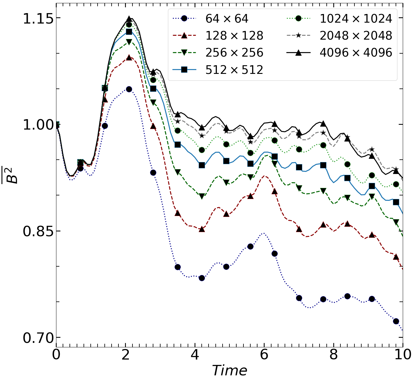
In the left panel of Fig. 1, we present the time evolution of in the non-resistive, ideal MHD simulations at various resolutions. The value of shows an increase as the resolution is enhanced (numerical resistivity decreases). This indicates that as the resolution increases, the curves exhibit greater convergence.
To determine the numerical resistivity at each resolution, we compare the time evolution of in ideal MHD simulations () and Res-MHD simulations at different physical resistivity values (e.g. , , and ). When the Res-MHD curve converges to the MHD curve, it indicates that the numerical resistivity is less than/equal to the physical resistivity.
For example, in the right panel of Fig. 1, we present the results of simulations at a resolution of grid cells. It is evident that the curve corresponding to converges to the MHD curve (). This convergence implies that the numerical dissipation at the resolution of grid cells is . Therefore, the resolutions grid cells can be suitable for studying the evolution and properties of the system.

In Fig.2 are shown the current densities in ideal MHD simulations in two resolutions at . The zoomed frames at the bottom show the reconnection layer in the middle of the simulation boxes. The left panel shows the results with the resolution of grid cells, where the numerical resistivity is less than so the current layer is thin enough to become plasmoid unstable. The right panel shows the results in lower resolution grid cells that give higher numerical resistivity (), the layer is thick and plasmoids do not emerge. We studied the magnetic reconnection and plasmoid formation in different models of resistive MHD, relativistic MHD, and 3D simulations in Kayanikhoo et al. (2023). In addition, Puzzoni2021 studied, the particle acceleration in the reconnection layer using PLUTO concerning the impact of Riemann solvers and reconstruction methods, grid resolutions, and numerical resistivity on particle acceleration in magnetic reconnection simulations. Their findings demonstrate that particle acceleration undergoes variations based on the choice of numerical solvers and Lundquist numbers ().


3.2 Energy conversion in MHD simulations
In this section, we study the magnetic energy dissipation in MHD and Res-MHD simulations. The conserved total energy density contains magnetic energy density , kinetic energy density , internal energy , and electric energy density .

We present the energy components that are computed at the resolution of grid cells in Fig. 3. The left column displays ideal MHD simulations (), while the right column represents Res-MHD simulations ().
In the top row of panels, we show the time evolution of magnetic energy. The magnetic energy increases to times its initial value at , coinciding with the presence of a current layer. Shortly after, at , plasmoids emerge within the current layer in the ideal MHD simulation (shown in Fig. 2). Subsequently, magnetic energy gradually dissipates as the simulation progresses. In the Res-MHD simulation, we note that the magnetic energy dissipates at a faster rate compared to the ideal MHD simulation.
In the second row of Fig.3, we show the average density of kinetic energy. The evolution of kinetic and magnetic energies illustrates that kinetic energy leads to the amplification of the magnetic field at approximately . Magnetic energy converts to kinetic energy through the magnetic reconnection to the time step .
Both kinetic and magnetic energies dissipate into internal energy by the end of the simulation time, heating the plasma, as shown in the third-row panels. It is evident that resistivity results in increased dissipation, causing internal energy to rise by approximately 0.5% more than in the ideal MHD simulation. The last row of panels represents electric energy, which evolves similarly to magnetic and kinetic energy, as expected.
4 Conclusions
In this paper, we investigated the magnetic energy evolution in the magnetized plasma by performing the Orszag-Tang (OT) test problem, in astrophysical magnetohydrodynamic (MHD) code PLUTO v. 4.4. OT is a standard test problem to test the power of MHD codes to capture shocks and resolve the substructures.
Using the resistive MHD module in PLUTO, we estimate the numerical dissipation in each resolution. The numerical resistivity in the resolution of grid cells is estimated to be which represents the lowest limit for the existence of the plasmoid-unstable current layer. In the ideal MHD simulation in the resolution of grid cells, the plasmoid-unstable current layer is observed while in the lower resolution, grid cells the plasmoids do not appear. Furthermore, our results confirm that in the Res-MHD simulation with a physical resistivity of , plasmoids do not emerge within the layer.
We studied the energy evolution in MHD and Res-MHD simulations. Our findings show that kinetic energy drives the amplification of the magnetic field, resulting in magnetic energy reaching approximately times its initial value. In MHD simulation, shortly after this increase, the plasmoids are observed within the current layer. Subsequently, both magnetic and kinetic energies gradually dissipate over the course of the simulation, with the dissipated energy converting into internal energy and heating the plasma. The results indicate that in resistive MHD simulation with resistivity , the dissipation is higher than in MHD simulation.
In Kayanikhoo et al. (2023), we further examined 3D simulations, compared relativistic and non-relativistic MHD simulations through energy conversion and magnetic reconnection rates, and the impact of resolution on reconnection rates in the models. Additionally, we compared two MHD codes widely used in astrophysics PLUTO and KORAL.
This project was funded by the Polish NCN grant No.2019/33/B/ST9/01564. MČ acknowledges the Czech Science Foundation (GAČR) grant No. 21-06825X. MW was supported by the European Research Council advanced grant âM2FINDERS - Mapping Magnetic Fields with INterferometry Down to Event hoRizon Scalesâ (Grant No. 101018682). High-resolution computations in this work were performed on the Prometheus and Ares machines, part of the PLGrid infrastructure.
References
- Akasofu (1968) Akasofu, S. (1968), Magnetospheric Substorm, pp. 212–253, Springer Netherlands, Dordrecht, ISBN 978-94-010-3461-6.
- Giovanelli (1946) Giovanelli, R. G. (1946), A theory of chromospheric flares, Nature Astronomy, 158(4003), pp. 81–82.
- Jiang and et al. (2021) Jiang, C. and et al. (2021), Nature Astronomy, 5(11), pp. 1126–1138.
- Kayanikhoo et al. (2023) Kayanikhoo, F., Cemeljic, M., Wielgus, M. and Kluzniak, W. (2023), Energy distribution and substructure formation in astrophysical mhd simulations, %****␣kay.bbl␣Line␣25␣****2308.16062.
- Loureiro et al. (2007) Loureiro, N. F., Schekochihin, A. A. and Cowley, S. C. (2007), Instability of current sheets and formation of plasmoid chains, Physics of Plasmas, 14(10), p. 100703, URL https://doi.org/10.10632F1.2783986.
- McPherron (1979) McPherron, R. L. (1979), Magnetospheric substorms, Reviews of Geophysics, 17(4), pp. 657–681.
- Mignone and et al. (2007) Mignone, A. and et al. (2007), Pluto: A numerical code for computational astrophysics, APJS, 170(1), pp. 228–242, astro-ph/0701854.
- Orszag and Tang (1979) Orszag, S. and Tang, C. M. (1979), Small-scale structure of two-dimensional magnetohydrodynamic turbulence, Journal of Fluid Mechanics, 90, pp. 129–143.
- Ripperda et al. (2020) Ripperda, B., Bacchini, F. and Philippov, A. A. (2020), Magnetic reconnection and hot spot formation in black hole accretion disks, The Astrophysical Journal, 900(2), p. 100, ISSN 1538-4357.
- Ripperda and et al. (2022) Ripperda, B. and et al. (2022), Black Hole Flares: Ejection of Accreted Magnetic Flux through 3D Plasmoid-mediated Reconnection, APJL, 924(2), L32, 2109.15115.