Generalized Finite Differences Method Applied to Finite Photonic Crystal

Abstract

We propose a Generalized Finite-Differences in the Frequency Domain method for the computation of photonic band structures of finite photonic crystals. Our approach is to discretize some fundamental domain instead of a single unit cell, such that boundary conditions of interest can be introduced into the eigenvalue problem. The validity and effectiveness of the proposed method are shown for the case of a one-dimensional photonic crystal embedded in an optical cavity. The limit from finite to infinite photonic crystals is reviewed in view of the proposed method.

[label1]organization=Grupo de Física Atómica y Molecular, Instituto de Física, Universidad de Antioquia, city=Medellín, country=Colombia

[label2]organization=Grupo de Óptica y Fotónica, Instituto de Física, Universidad de Antioquia, city=Medellín, country=Colombia

[label3]organization=Grupo de Superconductividad y Nanotecnología, Departamento de Física, Universidad Nacional de Colombia, city=Bogotá, country=Colombia

1 Introduction

In recent years, photonic crystals (PCs) have been demonstrated to exhibit unique properties that allow control of the light flow. These materials, characterized by their optical periodicity, have found widespread applications in various fields. For instance, PCs are used in realizing quantum optical phenomena [1, 2], designing quantum circuits [3], supercontinuum generation [4], fabrication of solar cells [5], biomedical and biological applications [6, 7], etc. On the other hand, the study and scope of applications of PCs are largely linked to proposing numerical solution methods. In literature, there are a vast number of methods for calculating PC properties, some of the newest being based on machine learning [8, 9]. Among the most widely known methods include the plane wave method (PWE) [10], the finite difference method in the time domain (FDTD) [11], and the finite difference method in the frequency domain (FDFD) [12].

The implementation of most of these methods relies on the validity on Bloch’s theorem, which is expected from the spatial periodicity and infinite spatial extension of the crystal. This theorem makes it possible to solve the computational problem in a single unit cell. Even when the system possesses a defect and does not exhibit strict periodicity, its properties can be approximated by the supercell method [13], whose efficiency is directly related to the size of the supercell.

However, recent technological advances that involve reducing systems to a nanoscopic scale or modeling realistic devices [14, 15] make Bloch’s theorem less rigorously applicable. For this reason, different methods have been studied to approach the finite PC problem. These methods are derived from rigorous treatments of the finite problem [16] or the use of techniques for infinite systems applied to the finite case [17] (usually considering Bloch waves).

Given the relevance of Bloch’s theorem and the advantages provided the FDFD method [18], it becomes valuable to identify the circumstances under which Bloch-type solutions remain valid in finite PCs since, in this case, they are not exactly eigenfunctions of the problem [19]. In this paper, we propose a novel method for the photonic band structure computation of finite PCs based on the validity of Bloch’s theorem in finite systems. The proposed method expands the scope of the FDFD method by allowing the introduction of more general boundary conditions. This enables photonic band gap analysis in the limit from finite to infinite PCs. We illustrate the effectiveness and validity of this method by examining the case of a one-dimensional finite PC inside an optical cavity.

2 Generalized FDFD Method

Before introducing the Generalized FDFD (GFDFD) method, let us briefly recall some things about the FDFD method. The FDFD method is a finite-differences method for the computation of PC eigenmodes that even allows supercell techniques to study crystal defects in the lattice [20]. This method reduces the problem of solving Maxwell equations in periodic dielectric media to the diagonalization of a single finite matrix. To quickly summarize how the method works, consider the decoupling of the time-independent Maxwell’s equations for the electric and magnetic fields

$$\mathcal{L}_{E}\mathbf{E} \triangleq\frac{1}{\epsilon}\nabla\times\left(\nabla\times\mathbf{E}\right)=\frac{\omega^{2}}{c^{2}}\mathbf{E},$$ (2.1a)

$$\mathcal{L}_{H}\mathbf{H} \triangleq\nabla\times\left(\frac{1}{\epsilon}\nabla\times\mathbf{H}\right)=\frac{\omega^{2}}{c^{2}}\mathbf{H},$$ (2.1b)

where $\mathcal{L}_{E}$ and $\mathcal{L}_{H}$ are linear differential operators on the fields, $\epsilon$ is the relative dielectric function characterizing the PC of interest, $\omega$ is the angular frequency of the fields and $c$ is the speed of light. These equations define a single eigenvalue problem from which one can obtain a set of eigenmodes, each with its corresponding eigenfrequency and field spatial profiles. Choosing to solve the eigenvalue problem for either $\mathcal{L}_{E}$ or $\mathcal{L}_{H}$ is a matter of convenience. However, the operator $\mathcal{L}_{H}$ is usually chosen since it is Hermitian, and the transversality condition for the magnetic field $\nabla\cdot\mathbf{H}=0$ is easier to work with [21]. Once an operator $\mathcal{L}$ is chosen, we define a sampling grid with $n$ points within a single unit cell of the crystal that allows one to represent the differential operator $\mathcal{L}$ by a $n\times n$ matrix $L$ up to an error due to discretization of space (see Figure 1). In principle, this truncation error can be arbitrarily reduced by using finer grids.

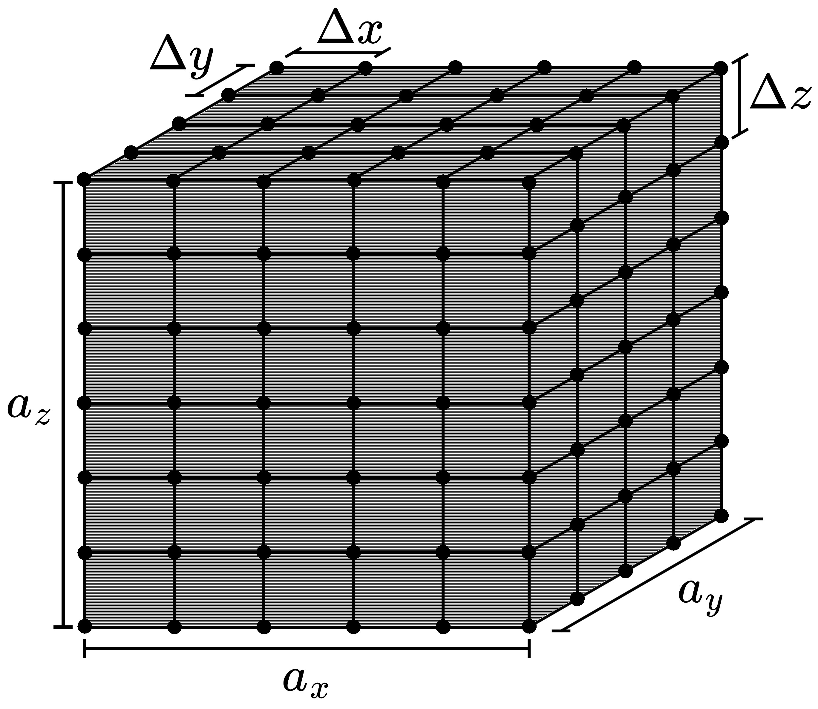
Figure 1: Sampling grid in a rectangular unit cell. Here $a_{x}$, $a_{y}$, and $a_{z}$ are the lattice parameters of the crystal and $\Delta x$, $\Delta y$ and $\Delta z$ are the sampling resolutions in each spatial axis. This discretization of space allows one to approximate linear differential operators by finite matrices up to a truncation error, which decreases with smaller sampling resolutions.

To properly define $L$, however, boundary conditions on the unit cell are needed. These are supplied by the fact that solutions to 2.1 can be labeled by a wave vector $\mathbf{k}$ in the First Brillouin Zone (FBZ) and satisfy the equations

$$\mathbf{E}_{\mathbf{k}}(\mathbf{r}+\mathbf{a}) =e^{i\mathbf{k}\cdot\mathbf{a}}\mathbf{E}_{\mathbf{k}}(\mathbf{r})$$ (2.2a)

$$\mathbf{H}_{\mathbf{k}}(\mathbf{r}+\mathbf{a}) =e^{i\mathbf{k}\cdot\mathbf{a}}\mathbf{H}_{\mathbf{k}}(\mathbf{r})$$ (2.2b)

for any arbitrary crystal lattice vector $\mathbf{a}$. The wave vector $\mathbf{k}$ is generally known as the crystal momentum. Equations 2.2 are also known as Bloch’s theorem or Bloch’s wave condition and are only valid if $\epsilon$ is a periodic function that extends through all space. Since this is the conventional way PCs are defined, the Bloch’s theorem can be naturally used and does not represent an actual constraint. Once $L$ is adequately defined, its eigenvalues and eigenvectors can be computed by modern numerical diagonalization methods, thus yielding an excellent approximation to the photonic band structure of the crystal and its corresponding eigenfunctions.

The FDFD method, as described above, allows one to study the optical properties of PCs that are infinitely extended through all space. Although, in reality, this is a physically impossible situation, methods based on this theoretical assumption still provide a realistic description of PCs. This is due to the fact that PCs are built such that the size of their unit cells is considerably small compared to the size of the crystals themselves. However, one can still ask for the possibility of studying periodic dielectric structures that do not necessarily extend endlessly through infinite space, such as real PCs embedded in optical cavities. With that in mind, we now propose a generalization of the FDFD method based on a slightly different discretization of space that allows a more general manipulation of the boundary conditions of the eigenvalue problem defined in Equations 2.1 while forcing Bloch’s wave condition. We will see how this generalization allows one to study Bloch waves in finite systems.

Our proposed generalization of the FDFD method goes as follows. We start by specifying a sampling grid with $N$ points within some fundamental domain instead of a single unit cell. This domain must comprise a finite amount $M$ of complete non-overlapping unit cells, each with $n$ sampling points, and is defined to include the boundary conditions of interest. For instance, to find the eigenmodes of the radiation field in a PC embedded in a resonant cavity, the whole cavity must be spatially sampled to apply reflective boundary conditions to the field. Again, this discretization of space and the boundary conditions allow us to represent the linear differential operator $\mathcal{L}$ as an $N\times N$ matrix $L$.

At this point, the eigenvalue problem can already be solved numerically. However, this may represent a great computational cost if either $M$ or $n$ are too large, and the solutions will not be, in general, Bloch waves. In order to filter out non-Bloch-type solutions and reduce the computational cost, we enforce the Bloch’s wave condition by expressing the field in all unit cells as phase-shifted copies of the field in a single unit cell (see Figure 2). This constraint reduces the number of independent variables from $N$ to $n$ and consequently the matrix $L$ can be transformed into an $n\times n$ matrix $\tilde{L}=B^{-1}LB$, where $B$ is defined as a $N\times n$ matrix by the equation

$$\left[\begin{array}[]{c}\psi_{0}\\ \psi_{1}\\ \vdots\\ \psi_{N-1}\\ \end{array}\right]=\sqrt{M}B\left[\begin{array}[]{c}\psi_{0}\\ \psi_{1}\\ \vdots\\ \psi_{n-1}\\ \end{array}\right],$$ (2.3)

and $B^{-1}$ is the left pseudo-inverse of $B$, which is simply its conjugate transpose. In principle, the boundary and the Bloch’s wave conditions are included in $\tilde{L}$, so the diagonalization of this matrix will yield the eigenmodes of the embedded PC. That is the essence of the GFDFD method. When $M=1$ and periodic boundary conditions are used, we return to the FDFD method. In this sense, the FDFD method is a particular case of the GFDFD method.

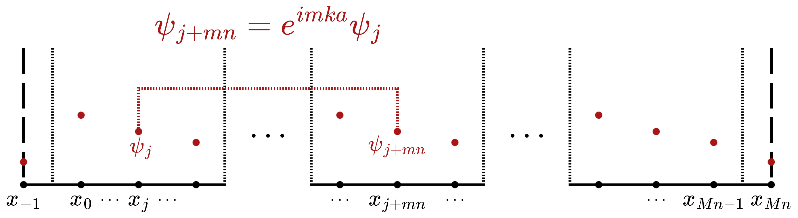
Figure 2: One-dimensional representation of a fundamental domain with $M$ unit cells and lattice constant $a$. Dashed and dotted dark vertical lines indicate the boundaries of the fundamental domain and the unit cells respectively. The field evaluated at point $x_{j}$ is denoted by $\psi_{j}$. Boundary conditions are applied at $x_{-1}$ and $x_{Mn}$. A red dashed line indicates the Bloch’s wave condition ($j=0,1,\dots,n-1$ and $m=0,1,\dots,M-1$), such that only $n$ values of the field are actually independent.

3 Photonic crystal in an optical cavity

To explicitly illustrate the method, the case of a one-dimensional finite bilayer crystal embedded in a cavity with metallic boundary conditions is studied. We considered a transverse mode of the electric field, in which case the discretization of Equation 2.1a takes the form

$$\sum_{j=0}^{n-1}L_{ij}E(x_{j})=-\frac{\omega^{2}}{c^{2}}E(x_{i}),$$ (3.1)

where $L_{ij}=(\delta_{i+1,j}-2\delta_{ij}+\delta_{i-1,j})/(\epsilon(x_{j})\Delta x^{2})$ and metallic boundary conditions are imposed by setting $\delta_{-1,j},\delta_{Mn,j}\rightarrow 0$. The diagonalization of the $Mn\times Mn$ matrix $L$ provides a complete set of eigenmodes of the radiation field in the cavity. These modes are computed to be later compared to those provided by the GFDFD method, which is implemented by the diagonalization of the $n\times n$ matrix $\tilde{L}=B^{-1}LB$, where

$$B=\frac{1}{\sqrt{M}}\left[\begin{array}[]{c}I_{n}\\ e^{ika}I_{n}\\ \vdots\\ e^{i(M-1)ka}I_{n}\\ \end{array}\right],$$ (3.2)

$I_{n}$ being the $n\times n$ identity matrix. At this stage, it is important to note that the GFDFD method relies on the validity of Bloch’s theorem in the fundamental domain. Consequently, all solutions provided by this method will exhibit periodicity in their amplitudes across all unit cells. This means only a subset of the complete set of solutions can be obtained for finite systems using the GFDFD method. This subset is specified by the node theorem as follows: let $\omega_{r}$ represent the $r$-th eigenvalue of the Sturm-Liouville problem defined by Equation 3.1. If the eigenvalues are labeled in increasing order ($\omega_{1}<\omega_{2}<\dots$), then it is well established that the $r$-th eigenfunction $\psi_{r}$ has exactly $r-1$ nodes [22]. Therefore, for a finite PC with $M$ unit cells, the eigenmode $\psi_{r}$ of $L$ can only exhibit periodic amplitude among all cells if $r$ is a multiple of $M$. This lets us filter out most non-Bloch-type solutions, allowing a more straightforward comparison between the eigenmodes of $L$ and $\tilde{L}$.

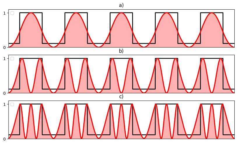
Figure 3: Red lines represent the normalized intensity profiles of the obtained solutions. (a), (b) and (c) correspond to the fifth, tenth, and fifteenth eigenmodes, respectively. The black line indicates the normalized dielectric profile.

The intensity profiles are presented in Figure 3 for the case of $M=5$ unitary cells. For this computation, we used $n=512$ sampling points per unit cell, a lattice constant of $a=1$, a wave number of $k=0$, and relative dielectric constants of 1 and 9. The profiles obtained from $\tilde{L}$ were almost indistinguishable to those given by $L$. This means that the GFDFD provides meaningful information about the actual eigenfrequencies of the system, even when Bloch’s theorem does not necessarily hold. Similar results are found for a higher number of unit cells, and the convergence of the method seems to depend mostly on the number $n$ of sampling points per unit cell. In Figure 4 we show how the mean relative convergence error (MRCE) of the first mode eigenfrequency, defined by

$$\text{MRCE}=\frac{a_{0}}{2\pi}\int_{\text{FBZ}}dk\left|\frac{\omega^{(n)}(k)-\omega^{(n-10)}(k)}{\omega^{(n)}(k)}\right|,$$ (3.3)

approaches zero as $n$ increases for all $M$, where $\omega^{(n)}(k)$ is the eigenfrequency of the first mode computed with $n$ sampling points per unit cell. The method converges quicker for lower values of $M$ and similar convergence results are obtained for higher modes.

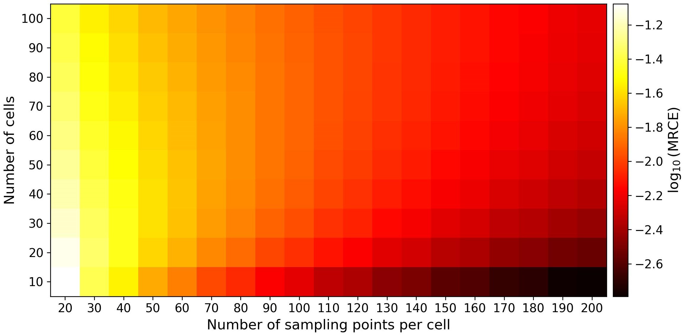
Figure 4: Convergence colormap of the GFDFD method. Color represents the logarithm of the MRCE. The method appears to converge for all number of cells.

To further study the validity of the method and the optical properties of PCs in the finite-to-infinite limit, we computed the photonic band structures of the system for increasing $M$ values. The band structure for a 1D infinite bilayer PC with the same lattice and dielectric constants is also computed using the PWE method. The results behave as expected: as $M$ increases, the band structure of the finite system converges to the one of the infinite system (see Figure 5). This is because as the number of cells increases, the ratio between the length of the crystal and the lattice constant increases as well, making the crystal effectively infinite compared to the dimensions of its unit cells. This convergence suggests that the crystal momentum, which is initially introduced by the enforcement of Bloch’s wave condition, acquires more physical relevance as the size of the crystal increases.

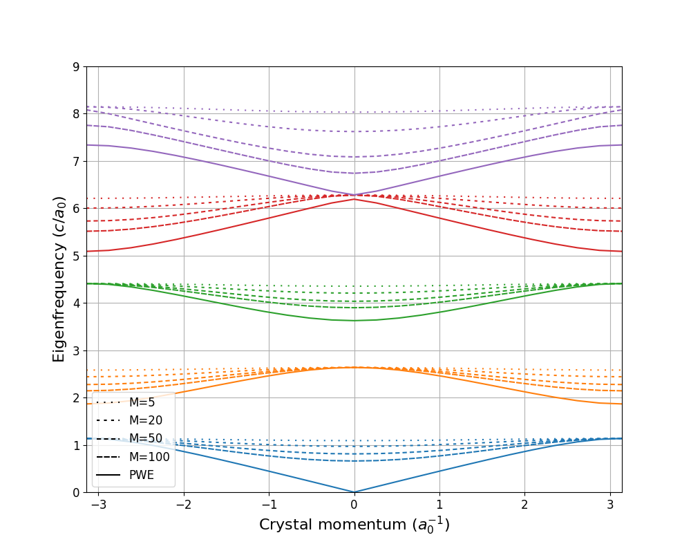
Figure 5: Photonic band structures of the one-dimensional infinite and finite bilayer PCs. Solid and dashed lines represent the solutions provided by the PWE and GFDFD methods for the infinite and finite systems respectively. The band structures were computed with 180 sampling points per unit cell.

4 Conclusions

We proposed and demonstrated a GFDFD method for the computation of the photonic band structures of finite PCs. This method, which strongly relies on the validity of Bloch’s theorem in finite systems, allows the calculation of Bloch-type solutions in finite systems. We particularly showed the method’s validity and efficacy by studying the eigenmodes of a one-dimensional finite bilayer PC embedded in an optical cavity. The intensity profiles of the radiation fields given by the GFDFD method showed a high resemblance to those obtained before using Bloch’s theorem, thus providing meaningful information about the actual eigenfrequencies of the composite system, with the addition of a new parameter of the set of solutions, namely the crystal momentum. This parameter, introduced by the enforcement of Bloch’s wave condition, appears to acquire more physical relevance as the size of the crystal increases, as suggested by the photonic band structure analysis in the finite-to-infinite limit. In this limit, the photonic band structure given by the GFDFD method for the finite PC appears to converge to that provided by the PWE method for the infinite PC, just as expected. This further solidifies the validity of the proposed method. As a perspective, we want to provide experimental support to the GFDFD method. We are also looking forward to explicitly demonstrate the validity of the method in two dimensions, showing particular cases of finite PCs in manifolds with non-trivial topologies, such as the Möbius Strip or the Klein Bottle, where boundary conditions on the fundamental domain are determined by the corresponding quotient space [23].

References

- [1] Sajeev John and Tran Quang. Spontaneous emission near the edge of a photonic band gap. Phys. Rev. A, 50:1764–1769, Aug 1994.
- [2] Sajeev John and Jian Wang. Quantum optics of localized light in a photonic band gap. Phys. Rev. B, 43:12772–12789, Jun 1991.
- [3] Jeremy L. O'Brien, Akira Furusawa, and Jelena Vučković. Photonic quantum technologies. Nature Photonics, 3(12):687–695, December 2009.
- [4] J. M. Dudley and J. R. Taylor, editors. Supercontinuum Generation in Optical Fibers. Cambridge University Press, April 2010.
- [5] Wei Liu, Hailing Ma, and Annika Walsh. Advance in photonic crystal solar cells. Renewable and Sustainable Energy Reviews, 116:109436, December 2019.
- [6] Huadong Chen, Rong Lou, Yanxiao Chen, Lili Chen, Jingya Lu, and Qianqian Dong. Photonic crystal materials and their application in biomedicine. Drug Delivery, 24(1):775–780, January 2017.
- [7] Xiaoren Lv, Bing Zhong, Yanfei Huang, Zhiguo Xing, Haidou Wang, Weiling Guo, Xueting Chang, and Zhinan Zhang. Research progress in preparation and application of photonic crystals. Chinese Journal of Mechanical Engineering, 36(1), March 2023.
- [8] Wei Ma, Zhaocheng Liu, Zhaxylyk A. Kudyshev, Alexandra Boltasseva, Wenshan Cai, and Yongmin Liu. Deep learning for the design of photonic structures. Nature Photonics, 15(2):77–90, October 2020.
- [9] Muhammad, John Kennedy, and C.W. Lim. Machine learning and deep learning in phononic crystals and metamaterials – a review. Materials Today Communications, 33:104606, December 2022.
- [10] Kazuaki Sakoda. Optical Properties of Photonic Crystals. Springer Berlin Heidelberg, 2005.
- [11] Allen Taflove and Susan Hagness. Computational electrodynamics. Artech House antennas and propagation library. Artech House, Norwood, MA, 3 edition, May 2005.
- [12] K. Ohtaka. Theory II: Advanced topics of photonic crystals. In Photonic Crystals, pages 65–118. Springer Berlin Heidelberg, 2004.
- [13] Liang Wu, Fie Zhuang, and Sailing He. Degeneracy analysis for a supercell of a photonic crystal and its application to the creation of band gaps. Phys. Rev. E, 67:026612, Feb 2003.
- [14] Kazuyoshi Hirose, Yong Liang, Yoshitaka Kurosaka, Akiyoshi Watanabe, Takahiro Sugiyama, and Susumu Noda. Watt-class high-power, high-beam-quality photonic-crystal lasers. Nature Photonics, 8(5):406–411, April 2014.
- [15] Takuya Inoue, Masahiro Yoshida, John Gelleta, Koki Izumi, Keisuke Yoshida, Kenji Ishizaki, Menaka De Zoysa, and Susumu Noda. General recipe to realize photonic-crystal surface-emitting lasers with 100-w-to-1-kw single-mode operation. Nature Communications, 13(1), July 2022.
- [16] Pedro Pereyra. The transfer matrix method and the theory of finite periodic systems. from heterostructures to superlattices. physica status solidi (b), 259(3), December 2021.
- [17] Zihao Chen, Xuefan Yin, Peishen Li, Zhao Zheng, Zixuan Zhang, Feifan Wang, and Chao Peng. Analytical theory of finite-size photonic crystal slabs near the band edge. Opt. Express, 30(9):14033–14047, Apr 2022.
- [18] Shangping Guo, Feng Wu, Sacharia Albin, and Robert S. Rogowski. Photonic band gap analysis using finite-difference frequency-domain method. Opt. Express, 12(8):1741–1746, Apr 2004.
- [19] Eougenious L Ivchenko and Grigory Pikus. Superlattices and other heterostructures. Springer Series in Solid-State Sciences. Springer, Berlin, Germany, 2 edition, February 2012.
- [20] Juan P. Vasco and Herbert Vinck-Posada. Método de diferencias finitas en el dominio de las frecuencias para cristales fotónicos 1d y 2d. TecnoLógicas, (24):125, June 2010.
- [21] John D. Joannopoulos, Steven G. Johnson, Joshua N. Winn, and Robert D. Meade. Photonic Crystals: Molding the Flow of Light (Second Edition). Princeton University Press, 2 edition, 2008.
- [22] G. Teschl. Ordinary Differential Equations and Dynamical Systems. Graduate studies in mathematics. American Mathematical Soc.
- [23] J Bělín, T Tyc, and S A R Horsley. Optical simulation of quantum mechanics on the möbius strip, klein’s bottle and other manifolds, and talbot effect. New Journal of Physics, 23(3):033003, mar 2021.