Abstract

In this paper, we explore the relativistic quantum motion of spin-zero scalar particles influenced by rainbow gravity’s in the background of a magnetic solution. Our focus is on the Bonnor-Melvin magnetic space-time, a four-dimensional solution featuring a non-zero cosmological constant. To analyze this scenario, we solve the Klein-Gordon equation using two sets of rainbow functions: (i) $f(\chi)=\frac{1}{(1-\beta\,\chi)}$, $h(\chi)=1$ and (ii) $f(\chi)=\frac{1}{(1-\beta\,\chi)}=h(\chi)$, where $0<\chi(=\frac{|E|}{E_{p}})\leq 1$ with $E_{p}$ being Planck’s energy. The resulting solutions provide the relativistic energy profiles of the scalar particles. Furthermore, we study the quantum oscillator fields through the Klein-Gordon oscillator within the same Bonnor-Melvin magnetic space-time background. Employing $f(\chi)=\frac{1}{(1-\beta\,\chi)}$, $h(\chi)=1$ as the rainbow function, we obtain the eigenvalue solutions for the quantum oscillator fields. Notably, we demonstrate that the relativistic energy profile of scalar particles and the oscillator fields are influenced by the topology of the geometry and the cosmological constant both are connected with the magnetic field strength. Additionally, we highlight the impact of the rainbow parameter on the energy profiles.

Faizuddin Ahmed
Department of Physics, University of Science & Technology Meghalaya, Ri-Bhoi, 793101, India
Abdelmalek Bouzenada
Laboratory of theoretical and applied Physics, Echahid Cheikh Larbi Tebessi University, Algeria

Keywords: Quantum fields in curved space-time; Relativistic wave equations; Solutions of wave equations: bound-states; special functions

PACS: 04.50.Kd; 04.62.+v; 03.65.Pm; 03.65.Ge; 02.30.Gp

1 Introduction

Engaging in a profound exploration of the intricate interplay between gravitational forces and the dynamics of quantum mechanical systems is a truly captivating pursuit. Albert Einstein’s groundbreaking general theory of relativity (GR) adeptly conceptualizes gravity as an inherent geometric aspect of spacetime [1]. This revolutionary theory unveils a fascinating connection between spacetime curvature and the emergence of classical gravitational fields, yielding precise predictions for phenomena like gravitational waves [2] and black holes [3]. Concurrently, the robust framework of quantum mechanics (QM) [4] provides invaluable insights into the subtle behaviors of particles at the microscopic scale. The convergence of these two foundational theories beckons us to delve into the profound mysteries situated at the crossroads of the macroscopic domain governed by gravity and the quantum intricacies of the subatomic realm.

Until a viable theory of quantum gravity (QG) is established, physicists are compelled to employ semi-classical approaches to QG. These approaches, while not providing a complete solution, prove beneficial in describing phenomena associated with extremely high-energy physics and the early universe [5, 6, 7, 8, 9, 10, 11, 12]. An illustrative instance of such a phenomenological or semi-classical approach to QG involves the infringement of Lorentz invariance. This entails deviating from the ordinary relativistic dispersion relation, brought about by modifying the physical energy and momentum at the Planck scale [13]. This departure from the dispersion relation has found application in diverse realms, including spacetime foam models [14], loop QG [15], spontaneous symmetry breaking of Lorentz invariance in string field theory [16], spin networks [17], discrete spacetime [18], as well as non-commutative geometry and Lorentz invariance violation [19].

Since then, scientists have delved into the myriad applications of rainbow gravity across various realms of physics. These explorations span a diverse array of topics, encompassing the isotropic quantum cosmological perfect fluid model within the framework of rainbow gravity [20], the adaptation of the Friedmann–Robertson–Walker universe in the context of Einstein-massive rainbow gravity [21], the thermodynamics governing black holes [22], the geodesic structure characterizing the Schwarzschild black hole [23, 24], and the nuanced examination of the massive scalar field in the presence of the Casimir effect [25].

Equally intriguing are inquiries into the impact of rainbow gravity on equilibrium configurations elucidated by the Tolman–Oppenheimer–Volkoff equation [26], the interplay between rainbow gravity and Hořava–Lifshitz gravity [27], the dynamic interplay of topology changes and the emergence of electric/magnetic charges due to quantum fluctuations in the context of rainbow gravity [28, 29], the effects arising from the combination of an f (R) theory with rainbow gravity on the computation of the induced cosmological constant [30], the calculation of black hole entropy utilizing the brick wall model in conjunction with a rainbow metric [31], considerations of zero-point energy, and the management of ultraviolet divergences through judicious selection of rainbow functions [32, 33, 34].

The exploration extends further to encompass topics such as rainbow gravity’s role in quantum cosmology [35], the intricate geometries of wormholes in both cis-Planckian and trans-Planckian regimes employing rainbow functions [36], the identification of temporal divergences for in-going observers in rainbow gravity beyond the Planck scale [37], and the dynamics of gravitational collapse within the framework of rainbow gravity [38]. These scholarly articles collectively underscore the growing interest in the semi-classical approach to rainbow gravity and highlight the potential applications of the findings presented in this paper, where we delve into the study of the Klein–Gordon (KG) oscillator within a space-time incorporating rainbow gravity and topological defects, specifically, a global monopole.

In recent years, a heightened interest has emerged in the exploration of magnetic fields, spurred by discoveries of systems with remarkably strong fields like magnetars [39, 40] and occurrences in heavy ion collisions [41, 42, 43]. This raises a compelling question: how can the magnetic field be seamlessly incorporated into the broader framework of general relativity, adding a fascinating dimension to the ongoing investigation of fundamental forces and their interconnected dynamics in the universe? The integration of the magnetic field within the framework of general relativity prompts intriguing questions, considering various existing solutions to the Einstein-Maxwell equations, including the Manko solution [44, 45], the Bonnor-Melvin universe [46, 47], and a recent proposal [48] that introduces the cosmological constant into the Bonnor-Melvin framework. Shifting focus to the intersection of general relativity and quantum physics raises another critical consideration: the potential interrelation of these two theories and its relevance. Numerous studies have tackled this inquiry, often relying on the Klein-Gordon and Dirac equations within curved space-times [49, 50]. This exploration spans diverse scenarios, from particles in Schwarzschild [51] and Kerr black holes [52] to cosmic string backgrounds [53, 54, 55], quantum oscillators [56, 57, 58, 59, 60, 61, 62, 63, 64], the Casimir effect [65, 66], and particles within the Hartle-Thorne space-time [67]. These investigations, alongside others [68, 69, 70], have provided valuable insights into how quantum systems respond to the arbitrary geometries of space-time. Consequently, an intriguing avenue of study involves examining quantum particles within a space-time influenced by a magnetic field. For instance, in [71], Dirac particles were explored in the Melvin metric, while our current work delves into the study of spin-0 bosons within a magnetic universe incorporating a cosmological constant, as proposed in [48].

The Melvin magnetic universe is an exact static solution of Einstein-Maxwell equations describe by the following metric in cylindrical coordinates is given by [47]

$$ds^{2}=\Lambda^{2}(r)\Big{(}-dt^{2}+dr^{2}+dz^{2}\Big{)}+\frac{r^{2}}{\Lambda^{2}(r)}\,d\phi^{2},$$ (1)

where $\Lambda(r)=\Big{(}1+K^{2}\,r^{2}\Big{)}$ with $K=\frac{B}{2}$ and $B$ is the magnetic field strength.

The Bonnor-Melvin universe with rainbow functions is described by the line-element

$$ds^{2}=-\frac{dt^{2}}{f^{2}}+\frac{1}{h^{2}}\Bigg{[}dz^{2}+\frac{1}{2\,\Lambda}\,\Big{(}d\rho^{2}+\alpha^{2}\,\sin^{2}\rho\,d\phi^{2}\Big{)}\Bigg{]},$$ (2)

where $\Lambda$ denotes the cosmological constant, and $\alpha$ represents a constant of integration. For $f\to 1$ and $h\to 1$, we will get back the original Bonnor-Melvin magnetic universe [48]. The magnetic field strength for this modified space-time is given by $\mathcal{H}=\frac{\alpha}{h(\chi)\,\sqrt{2}}\,\sin\rho$ which is influenced by the rainbow function in addition to those parameters $\alpha,\Lambda$. Here the rain bow functions $f=f(\chi)$, $h=h(\chi)$, where $\chi=\frac{|E|}{E_{p}}$ with $E_{p}$ being Planck’s energy.

The covariant ($g_{\mu\nu}$) and contravariant form ($g_{\mu\nu}$) of the metric tensor for the space-time (3) are given by

$$g_{\mu\nu}=\begin{pmatrix}-\frac{1}{f^{2}}&0&0&0\\ 0&\frac{1}{2\,\Lambda\,h^{2}}&0&0\\ 0&0&\frac{\alpha^{2}\,\sin^{2}r}{2\,\Lambda\,h^{2}}&0\\ 0&0&0&\frac{1}{h^{2}}\end{pmatrix},\quad g^{\mu\nu}=\begin{pmatrix}-f^{2}&0&0&0\\ 0&2\,\Lambda\,h^{2}&0&0\\ 0&0&\frac{2\,\Lambda\,h^{2}}{\alpha^{2}\,\sin^{2}r}&0\\ 0&0&0&h^{2}\end{pmatrix}.$$ (3)

The determinant of the metric tensor for the space-time (4) is given by

$$det\,(g_{\mu\nu})=g=-\frac{\alpha^{2}\,f^{2}}{4\,\Lambda^{2}\,h^{6}}\,\sin^{2}r\,.$$ (4)

Our motivation is to study the relativistic quantum motions of scalar particles under the influence of rainbow gravity’s in the background of a Bonnor-Melvin solution. This is a four-dimensional space-time with a cosmological constant attached with the magnetic field strength along $z$-direction. We derive the radial equation in this magnetic universe background and obtain approximate as well as exact analytical eigenvalue solutions by choosing two pairs of rainbow functions: ((i) $f(\chi)=\frac{1}{1-\beta\,\chi}$, $h(\chi)=1$ [72] and (ii) $f(\chi)=\frac{1}{1-\beta\,\chi}=h(\chi)$ [73, 74, 75]. Afterwards, we study the relativistic quantum oscillator fields in the background of same geometry with one pair of rainbow gravity’s function $f(\chi)=\frac{1}{1-\beta\,\chi}$, $h(\chi)=1$ and obtain the approximate energy profiles. In fact, we show that the energy profiles of scalar and oscillator fields are influenced by the topology of the space-time and the cosmological constant. Furthermore. rainbow parameter modifies the energy spectrum and shifted the results.

This paper is summarized as follows: In section 2, we study the Klein-Gordon equation in the background of Bonnor-Melvin magnetic universe with a cosmological constant in the presence of rainbow gravity’s. We derive the radial equation obtain the approximate as well as analytical solutions by choosing two pairs of rainbow functions. In section 3, we study the relativistic quantum oscillator fields in the same magnetic universe background and obtain the approximate eigenvalue solution by choosing on pair of rainbow functions. In section 4, we present our results and discussion. Throughout this paper, we use the system of units, where $c=1=G$.

2 Effects of rainbow gravity on scalar fields in magnetic universe background

Therefore, the relativistic wave equation describing the quantum system is given by [76]

$$\Bigg{[}-\frac{1}{\sqrt{-g}}\,\partial_{\mu}\,\Big{(}\sqrt{-g}\,g^{\mu\nu}\,\partial_{\nu}\Big{)}+M^{2}\Bigg{]}\,\Psi=0,$$ (5)

where $M$ is the rest mass of the particles, $g$ is the determinant of the metric tensor $g_{\mu\nu}$ with its inverse $g^{\mu\nu}$.

Therefore, the KG-equation (5) in the space-time (2) becomes can be expressed in the following differential equation:

$$\Bigg{[}-f^{2}\,\frac{d^{2}}{dt^{2}}+2\,\Lambda\,h^{2}\,\Bigg{\{}\frac{d^{2}}{dr^{2}}+\frac{1}{\tan r}\,\frac{d}{dr}+\frac{1}{\alpha^{2}\,\sin^{2}r}\,\frac{d^{2}}{d\phi^{2}}\Bigg{\}}+h^{2}\,\frac{d^{2}}{dz^{2}}-M^{2}\Bigg{]}\,\Psi=0\,.$$ (6)

In quantum mechanical system, the total wave function is always expressible in terms of different variables. In our case, we choose the following ansatz of the total wave function $\Psi$ in terms of different variable functions $\psi(x)$ and $\Theta(\theta)$ as follows:

$$\Psi=\exp(-i\,E\,t)\,\exp(i\,m\,\phi)\,\exp(i\,k\,z)\,\psi(r),$$ (7)

where $E$ is the particles energy, $m=0,\pm\,1,\pm\,2,....$ are the eigenvalues of the angular quantum number. We are able to express total wave function in the above since the differential equation (6) is independent of the time $t$, angular $\phi$ coordinates, and $z$ coordinate.

Substituting the total wave function (7) into the differential equation (6) and after separating the variables, we obtain the differential equations for $\psi(x)$ as follows:

$$\psi^{\prime\prime}+\frac{1}{\tan r}\,\psi^{\prime}+\Bigg{[}\frac{(f^{2}\,E^{2}-M^{2})}{2\,\Lambda\,h^{2}}-\frac{k^{2}}{2\,\Lambda}-\frac{\iota^{2}}{\sin^{2}r}\Bigg{]}\,\psi=0,$$ (8)

where $\iota=\frac{|m|}{|\alpha|}$.

2.1 Approximation Analytical solution

In this part, we solve the above equation taking an approximation of the trigonometric function up to the first order, that is, $\sin r\approx r$, $\tan r\approx r$. Therefore, the radial wave equation (8) reduces to the following form:

$$\psi^{\prime\prime}+\frac{1}{r}\,\psi^{\prime}+\Bigg{[}\frac{(f^{2}\,E^{2}-M^{2})}{2\,\Lambda\,h^{2}}-\frac{k^{2}}{2\,\Lambda}-\frac{\iota^{2}}{r^{2}}\Bigg{]}\,\psi=0.$$ (9)

This is Bessel differential equation whose solutions are well-know. We want a solution which is finite at the origin $r=0$ and this is possible when we write

$$\psi(r)=c_{1}\,J{\iota}(r\,\Theta),\quad\Theta=\frac{(f^{2}\,E^{2}-M^{2})}{2\,\Lambda\,h^{2}}-\frac{k^{2}}{2\,\Lambda},$$ (10)

where $c_{1}$ is an arbitrary constant.

Asymptotic form of the Bessel function [77, 78] is given by

$$J_{\iota}(r\,\Theta)\propto\cos\Big{(}r\,\Theta-\frac{\iota\,\pi}{2}-\frac{\pi}{4}\Big{)}$$ (11)

Now, we impose a hard wall confining potential condition which states that at some axial distance $r=r_{0}>0$, the radial wave function $\psi(r=r_{0})=0$. This condition is also known as Dirichlet’s boundary condition. Therefore, substituting (11) into the equation (10) and using this condition $\psi(r=r_{0})=0$, we obtain the following relation of the energy spectrum given by

$$f^{2}\,E^{2}=M^{2}+h^{2}\,\Bigg{[}k^{2}+\Lambda\,\Big{(}2\,n+\frac{3}{2}+\frac{|m|}{|\alpha|}\Big{)}^{2}\,\frac{\pi^{2}}{2\,r^{2}_{0}}\Bigg{]},$$ (12)

where $n=0,1,2,3,....$.

Now, we use two different types of rainbow function and obtain the compact expression of the energy eigenvalue.

Case A: Rainbow functions $f(\chi)=\frac{1}{1-\beta\,\chi}$, $h(\chi)=1$, and $\chi=\frac{|E|}{E_{p}}$

Substituting this pair of rainbow function into the expression (12) and after simplification, we obtain

$$E_{n,m}=\Bigg{[}\frac{\beta}{E_{p}}\pm\Bigg{\{}M^{2}+k^{2}+2\,\Lambda\,\Big{(}n+\frac{3}{4}+\frac{|m|}{2|\alpha|}\Big{)}^{2}\,\frac{\pi^{2}}{r^{2}_{0}}\Bigg{\}}^{-1/2}\Bigg{]}^{-1}.$$ (13)

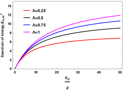
(a)

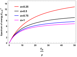
(b)

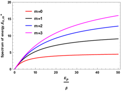
(c)

Figure 1: The energy spectrum $E_{m,n}^{+}$ for the relation given in Equation (13), where the parameters are set as $k=M=1,n=0,r_{0}=0.5$.

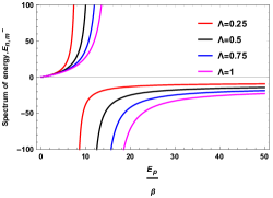
(d)

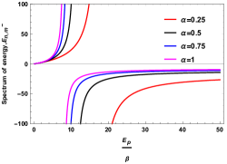
(e)

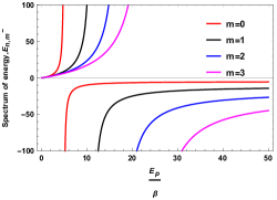
(f)

Figure 2: The energy spectrum $E_{m,n}^{-}$ for the relation given in Equation (13), where the parameters are set as $k=M=1,n=0,r_{0}=0.5$

Equation (13) is the relativistic energy profile of a scalar particle in the background of magnetic universe with non-zero cosmological constant. We see that the relativistic energy spectrum is influenced by the topology of the geometry characterized by the parameter $\alpha$ and the cosmological constant $\Lambda$. Furthermore, the rainbow parameter $\beta<1$ also modified the energy profiles and shifted the results.

We have presented Figure 1, illustrating the energy spectrum $E_{n,m}(+)$ (considering the positive sign within the brackets in the energy expression 13) plotted against $E_{p}/\beta$. The figure encompasses different values of the cosmological constant (Fig: 1(a)), the topology parameter $\alpha$ (Fig: 1(b)), and the angular quantum number $m$ (Fig: 1(c)). Notably, the nature of the spectrum is parabolic and exhibits an upward shift with increasing values of $\Lambda$ and $m$, while depicting a decreasing trend for $\alpha$. In Figure 2, we depict the spectrum of energy $E_{n,m}(-)$, this time considering the minus sign within the brackets in the energy expression 13.

Case B: Rainbow functions $f(\chi)=\frac{1}{1-\beta\,\chi}=h(\chi)$

Substituting this pair of rainbow function into the expression (12) and after simplification, we obtain

$$E_{n,m}=\frac{1}{\Big{(}1-\frac{M^{2}\,\beta^{2}}{E^{2}_{p}}\Big{)}}\,\Bigg{[}-\frac{\beta\,M^{2}}{E_{p}}\pm\sqrt{M^{2}+\Big{(}1-\frac{M^{2}\,\beta^{2}}{E^{2}_{p}}\Big{)}\,\Bigg{\{}k^{2}+2\Lambda\Big{(}n+\frac{3}{4}+\frac{|m|}{2|\alpha|}\Big{)}^{2}\,\frac{\pi^{2}}{r^{2}_{0}}\Bigg{\}}}\Bigg{]}.$$ (14)

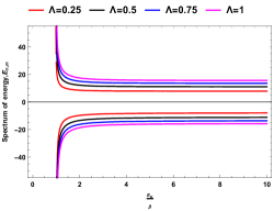
(a)

(b)

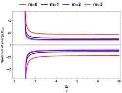
(c)

Figure 3: The energy spectrum $E_{m,n}^{+}$ for the relation given in Equation (14), where the parameters are set as $k=M=1,n=0,r_{0}=0.5$.

Equation (14) is the relativistic energy profile of a scalar particle in the background of magnetic universe with non-zero cosmological. We see that the relativistic energy spectrum is influenced by the topology of the geometry characterized by the parameter $\alpha$ and the cosmological constant $\Lambda$.

We present Figure 3, illustrating the energy spectrum $E_{n,m}(+)$ (considering the positive sign within the brackets in the energy expression 14) plotted against $E_{p}/\beta$. The figure displays various values of the cosmological constant (Fig: 3(a)), the topology parameter $\alpha$ (Fig: 3(b)), and the angular quantum number $m$ (Fig: 3(c)).

2.2 Exact analytical solution

In this part, we solve the above differential equation (8) by analytical treatment. Transforming to a new variable via $\cos r=u$ into the equation (8), we obtain

$$(1-u^{2})\,\psi^{\prime\prime}(u)-2\,u\,\psi^{\prime}(u)+\Big{[}\Theta-\frac{\iota^{2}}{1-u^{2}}\Big{]}\,\psi(u)=0,$$ (15)

where $\Theta=\frac{(f^{2}\,E^{2}-M^{2})}{2\,\Lambda\,h^{2}}-\frac{k^{2}}{2\,\Lambda}$.

Setting $\ell=(\Theta+\frac{1}{4})^{1/2}-\frac{1}{2}$, where $\ell\,(\ell+1)=\Theta$, one can write the above equation into the standard differential equation form given by

$$(1-u^{2})\,\psi^{\prime\prime}(u)-2\,u\,\psi^{\prime}(u)+\Bigg{[}\ell\,(\ell+1)-\frac{\iota^{2}}{1-u^{2}}\Bigg{]}\,\psi(u)=0,$$ (16)

Equation (16) is the associated Legendre polynomial whose solution is well-known given by [77, 78]

$$\psi(u)=P^{\iota}_{\ell}(u)=(-1)^{\iota}\,(1-u^{2})^{\iota/2}\,\frac{d^{\iota}}{du^{\iota}}\left(P_{\ell}(u)\right),$$ (17)

where $P_{\ell}(u)$ is the Legendre polynomials.

It is well-known that the associated Legendre polynomial can be expressed in terms of hypergeometric function as follows [77]:

$$p^{\iota}_{\ell}(u)=\frac{1}{\Gamma(1-\iota)}\,\Big{(}\frac{1+u}{1-u}\Big{)}^{\iota/2}\,{}_{2}F_{1}\left(-\ell,\ell+1;1-\iota;\frac{1-u}{2}\right).$$ (18)

Also, we know that the power series expansion of hypergeometric function terminates to a finite degree polynomial provided $-\ell$ must be a non-positive integer, that means, $\ell=n$ [77], where $n=0,1,2,3,...$. Thus, we can write $\Theta=n\,(n+1)$ and simplification of this condition results the following relation of the energy eigenvalue

$$f^{2}\,E^{2}=M^{2}+h^{2}\,\Big{[}k^{2}+2\,\Lambda\,n\,(n+1)\Big{]},\quad n=0,1,2,.....$$ (19)

It is interesting to note here that the relativistic energy eigenvalue expression $E$ of a scalar particle obtain from the above relation (19) for any pair of rainbow function is independent of the geometrical topology characterized by the parameter $\alpha$. Now, we use two pairs of rainbow function mentioned earlier and obtain the compact expression of the energy eigenvalue.

Case A: Rainbow functions $f(\chi)=\frac{1}{1-\beta\,\chi}$, $h(\chi)=1$

Substituting this pair of rainbow function into the expression (19) and after simplification, we obtain

$$E_{n}=\Bigg{[}\frac{\beta}{E_{p}}\pm\Big{\{}M^{2}+k^{2}+2\,\Lambda\,n\,(n+1)\Big{\}}^{-1/2}\Bigg{]}^{-1}.$$ (20)

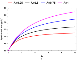
(a)

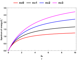
(b)

Figure 4: The energy spectrum $E_{m,n}^{+}$ for the relation given in Equation(20), where the parameters are set as $k=M=1$.

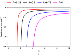
(a)

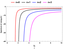
(b)

Figure 5: The energy spectrum $E_{m,n}^{-}$ for the relation given in Equation(20), where the parameters are set as $k=M=1$.

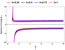
(a)

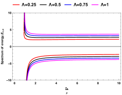
(b)

Figure 6: The energy spectrum $E_{m,n}$ for the relation given in Equation (21), where the parameters are set as $k=M=1$.

Equation (20) is the relativistic energy profile of a scalar particle in the background of magnetic universe with non-zero cosmological. We see that the relativistic energy spectrum is influenced by the cosmological constant $\Lambda$ and the rainbow parameter $\beta$.

We present Figure 4, displaying the energy spectrum $E_{n,m}(+)$ (considering the positive sign within the brackets in the energy expression 20) plotted against $E_{p}/\beta$. The figure encompasses different values of the cosmological constant (Fig: 4(a)) and the radial quantum number $n$ (Fig: 4(b)). Notably, the nature of the spectrum is parabolic and demonstrates an upward shift with increasing values of $\Lambda$ and $n$. Figure 5 illustrates the spectrum of energy $E_{n,m}(-)$ (considering the negative sign within the brackets in the energy expression 20), plotted against $E_{p}/\beta$. The figure features various values of the cosmological constant (Fig: 5(a)) and the radial quantum number $n$ (Fig: 5(b)).

Case B: Rainbow functions $f(\chi)=\frac{1}{1-\beta\,\chi}=h(\chi)$

Substituting this pair of rainbow function into the expression (19) and after simplification, we obtain

$$E_{n}=\frac{1}{\Big{(}1-\frac{M^{2}\,\beta^{2}}{E^{2}_{p}}\Big{)}}\,\Bigg{[}-\frac{\beta\,M^{2}}{E_{p}}\pm\sqrt{M^{2}+\Big{(}1-\frac{M^{2}\,\beta^{2}}{E^{2}_{p}}\Big{)}\,\Big{(}k^{2}+2\,\Lambda\,n\,(n+1)\Big{)}}\Bigg{]}.$$ (21)

Equation (21) is the relativistic energy profile of a scalar particle in the background of magnetic universe with non-zero cosmological. We see that the relativistic energy spectrum is influenced by the cosmological constant $\Lambda$ and the rainbow parameter $\beta$.

We present Figure 6, displaying the energy spectrum $E_{n,m}(+)$ (considering the positive sign within the brackets in the energy expression 21) plotted against $E_{p}/\beta$. The figure encompasses different values of the cosmological constant for $n=1$ (Fig: 6(a)) and for $n=2$ (Fig: 6(b)).

3 Effects of rainbow gravity on oscillator fields in magnetic universe background

In this part, we study the relativistic quantum oscillator fields via the Klein-Gordon oscillator in the background of Bonnor-Melvin magnetic universe. This oscillator field is studied by replacing the momentum operator into the Klein-Gordon equation via $\partial_{\mu}\to(\partial_{\mu}+M\,\omega\,X_{\mu})$, where the four-vector $X_{\mu}=(0,r,0,0)$ and $\omega$ is the oscillator frequency. The relativistic quantum oscillator fields in curved space-times background have been investigated by numerous authors (see, [56, 57, 58, 59, 60, 61, 62, 63, 64]).

Therefore, the relativistic wave equation describing the quantum oscillator fields is given by

$$\Big{[}\frac{1}{\sqrt{-g}}\,(\partial_{\mu}+M\,\omega\,X_{\mu})\,(\sqrt{-g}\,g^{\mu\nu})\,(\partial_{\nu}-M\,\omega\,X_{\nu})\Big{]}\,\Psi=M^{2}\,\Psi.$$ (22)

Expressing the wave equation (22) in the magnetic universe background (2), we obtain

$$\Bigg{[}-f^{2}\,\frac{d^{2}}{dt^{2}}+2\,\Lambda\,h^{2}\,\Bigg{\{}\frac{d^{2}}{dr^{2}}+\frac{1}{\tan r}\,\frac{d}{dr}-M\,\omega-\frac{M\,\omega\,r}{\tan r}-M^{2}\,\omega^{2}\,r^{2}+\frac{1}{\alpha^{2}\,\sin^{2}r}\,\frac{d^{2}}{d\phi^{2}}\Bigg{\}}$$

$$+h^{2}\,\frac{d^{2}}{dz^{2}}-M^{2}\Bigg{]}\,\Psi=0\,.$$ (23)

Substituting the wave function ansatz (7) into the above differential equation (23) results the following second-order differential equation form:

$$\psi^{\prime\prime}+\frac{1}{\tan r}\,\psi^{\prime}+\Bigg{[}\frac{(f^{2}\,E^{2}-M^{2})}{2\,\Lambda\,h^{2}}-M\,\omega-\frac{M\,\omega\,r}{\tan r}-M^{2}\,\omega^{2}\,r^{2}-\frac{k^{2}}{2\,\Lambda}-\frac{\iota^{2}}{\sin^{2}r}\Bigg{]}\,\psi=0.$$ (24)

We solve the above equation by taking an approximation of the trigonometric function up to the first order, that is, $\sin r\approx r$, $\tan r\approx r$. Therefore, the radial wave equation (24) reduces to the following form:

$$\psi^{\prime\prime}+\frac{1}{r}\,\psi^{\prime}+\Bigg{[}\lambda-M^{2}\,\omega^{2}\,r^{2}-\frac{\iota^{2}}{r^{2}}\Bigg{]}\,\psi=0,$$ (25)

where $\lambda=\frac{(f^{2}\,E^{2}-M^{2})}{2\,\Lambda\,h^{2}}-\frac{k^{2}}{2\,\Lambda}-2\,M\,\omega$.

Transforming to a new variable via $s=M\,\omega\,r^{2}$ into the above equation (25) results the following equation form [79]:

$$\psi^{\prime\prime}(s)+\frac{(c_{1}-\,c_{2}\,s)}{s\,(1-c_{3}\,s)}\,\psi^{\prime}(s)+\frac{\Big{(}-\xi_{1}\,s^{2}+\xi_{2}\,s-\xi_{3}\Big{)}}{s^{2}\,(1-c_{3}\,s)^{2}}\,\psi(s)=0,$$ (26)

where $c_{1}=1$, $c_{2}=0=c_{3}$ and

$$\xi_{1}=\frac{1}{4},\quad\xi_{2}=\frac{\lambda}{4\,M\,\omega},\quad\xi_{3}=\frac{\iota^{2}}{4}.$$ (27)

Therefore, the energy eigenvalue relation will be

$$f^{2}\,E^{2}=M^{2}+h^{2}\,\Bigg{[}k^{2}+8\,M\,\omega\,\Lambda\,\Big{(}n+1+\frac{|m|}{2|\alpha|}\Big{)}\Bigg{]},\quad n=0,1,2,....$$ (28)

The corresponding radial wave function will be

$$\psi(s)=\mathcal{N}\,s^{\frac{|m|}{2|\alpha|}}\,e^{-s/2}\,L^{\frac{|m|}{|\alpha|}}_{n}(s),$$ (29)

where $\mathcal{N}$ is the normalization constant. The normalization constant cab be determined using hte following relation

$$\frac{|\alpha|}{2\,\Lambda}\,\int^{\infty}_{0}\,r\,|\psi(r)|^{2}\,dr=1.$$ (30)

Here, we use only one pair of the rainbow function given by

$$f(\chi)=\frac{1}{1-\beta\,\chi},\quad h(\chi)=1,\quad\chi=\frac{|E|}{E_{p}}.$$ (31)

Substituting this rainbow function into the relation (28) and after simplification, we obtain

$$E_{n,m}=\Bigg{[}\frac{\beta}{E_{p}}\pm\Bigg{\{}M^{2}+k^{2}+8\,M\,\omega\,\Lambda\,\Big{(}n+1+\frac{|m|}{2|\alpha|}\Big{)}\Bigg{\}}^{-1/2}\Bigg{]}^{-1}.$$ (32)

(a)

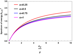
(b)

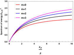
(c)

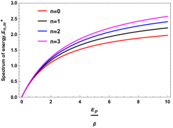
(d)

Figure 7: The energy spectrum $E_{m,n}^{+}$ for the relation given in Equation (32), where the parameters are set as $k=M=1$ and $\omega=0.5$.

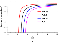
(e)

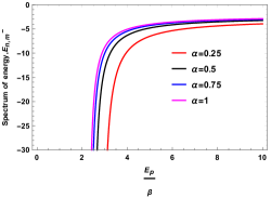
(f)

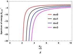
(g)

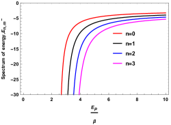
(h)

Figure 8: The energy spectrum $E_{m,n}^{-}$ for the relation given in Equation (32), where the parameters are set as $k=M=1$ and $\omega=0.5$.

Equation (32) is the relativistic energy profile of oscillator fields in the background of a magnetic universe with non-zero cosmological. We see that the relativistic energy spectrum is influenced by the topology of the geometry characterized by the parameter $\alpha$, the cosmological constant $\Lambda$, and the rainbow parameter $\beta$.

We present Figure 7, displaying the energy spectrum $E_{n,m}(+)$ (positive sign within the brackets in the energy expression 32) plotted against $E_{p}/\beta$. The figure encompasses various values of the cosmological constant (Fig: 7(a)), topology parameter (Fig: 7(b)), angular quantum number (Fig: 7(c)), and radial quantum number (Fig: 7(d)). It is observed that the energy spectrum exhibits a parabolic nature and shifts upward with increasing values of these parameters ($\Lambda,m,n$), except in Figure 7(b) where a decreasing trend is observed with increasing $\alpha$. Figure 8 illustrates the energy spectrum $E_{n,m}(-)$ (minus sign within the brackets in the energy expression 32) and encompasses different values of the cosmological constant (Fig: 8(a)), topology parameter (Fig: 8(b)), angular quantum number (Fig: 8(c)), and radial quantum number (Fig: 8(d)).

4 Conclusions

The exploration of wave equations, including the Schrödinger equation, the Klein-Gordon equation, and the Duffin-Kemmer-Petiau equation within the framework of curved space, has been a long-standing research interest. Numerous scholars have delved into these wave equations within the backdrop of topological defects, demonstrating that these defects induce modifications in the eigenvalue solutions.

In this analysis, our emphasis was on an Einstein-Maxwell solution of the field equations that incorporates a cosmological constant. Specifically, we selected the Bonnor-Melvin solution-a four-dimensional magnetic universe characterized by a magnetic field strength contingent upon the topology of the geometry. Subsequently, we studied the quantum motion of charge-free scalar particles, as described by the Klein-Gordon equation, within this chosen framework. Importantly, our entire investigation was carried out under the influence of rainbow gravity’s. As a result, the magnetic field strength alters by the rainbow gravity’s.

In Section 2, we derived the radial equation and established approximate and exact eigenvalue relations through special functions. We employed two categories of rainbow functions and showcased the relativistic energy profiles of charge-free scalar particles for each set of rainbow functions, as expressed in equations (13)–(14) and (20)–(21). Our analysis showed that the energy profiles undergo modifications influenced by the topology of the geometry ($\alpha$), the cosmological constant ($\Lambda$), and the rainbow parameter ($\beta$). To illustrated these spectrum of energy, we generated Figures 1–6 showing these for different values of the cosmological constant, topology parameter, angular quantum number, and radial quantum number and found interesting results.

In Section 3, our focus shifted to the investigation of quantum oscillator fields within the background of the same magnetic universe considering the influence of rainbow gravity. We derived the radial equation governing the oscillator fields and proceeded to solve it employing special functions. The approximate energy eigenvalue was determined by utilizing a specific pair of rainbow functions given in equation (32). Once again, we observed that the relativistic energy spectrum of oscillator fields is subject to modification, impacted by the topology of the geometry ($\alpha$), the cosmological constant ( $\Lambda$), and the rainbow parameter ($\beta$). Additionally, the oscillator frequency ($\omega$) also contributes to alterations in the energy profile. To illustrated spectrum of energy, we generated Figures 7–8 showing these for different values of the cosmological constant, topology parameter, angular quantum number, and radial quantum number and found interesting results.

In summary, we investigated quantum field in curved space-time background in the context of rainbow gravity’s. This curved space-time is the Bonnor-Melvin magnetic universe produced by a magnetic field strength along the symmetry axis $z$-direction taking into account the cosmological constant $\Lambda>0$. The present experimental observation confirms that expanding of the universe is accelerating. we have shown that the quantum dynamics of scalar charge-free particles are influenced and results get modified.

Conflict of Interest

There is no conflict of interests.

Funding Statement

There is no funding agency associated with this manuscript.

Data Availability Statement

No data were generated or analysed during this study.

References

- [1] A. Einstein, Annalen Phys. 49, 769 (1916) https://doi.org/10.1002/20andp.200590044.
- [2] B. P. Abbott et al, Phys Rev Lett 116, 061102 (2016) https://doi.org/10.1103/PhysRevLett.116.061102.
- [3] K. Akiyama et al, Astrophys J Lett 875, L1 (2019) https://doi.org/10.3847/2041-8213/ab0f43.
- [4] R. P. Feynman, and A. R. Hibbs, Quantum mechanics and path integrals, Dover Publications Inc. (1965).
- [5] G. Amelino-Camelia, Phys. Lett. B 510, 255 (2001) https://doi.org/10.1016/S0370-2693(01)00506-8.
- [6] G. Amelino-Camelia, Int. J. Mod. Phys. D 11, 35 (2002) https://doi.org/10.1142/S0218271802001330.
- [7] G. Amelino-Camelia, J. Kowalski-Glikman, G. Mandanici, A. Procaccini, Int. J. Mod. Phys. A 20, 6007 (2005) https://doi.org/10.1142/S0217751X05028569.
- [8] J. Magueijo, L. Smolin, Phys. Rev. Lett. 88, 190403 (2002) https://doi.org/10.1103/PhysRevLett.88.190403.
- [9] J. Magueijo, L. Smolin, Phys. Rev. D 67, 044017 (2003) https://doi.org/10.1103/PhysRevD.67.044017.
- [10] L. Smolin, Nucl. Phys. B 742, 142 (2006) https://doi.org/10.1016/j.nuclphysb.2006.02.017.
- [11] S. Ghosh, Phys. Rev. D 74, 084019 (2006) https://doi.org/10.1103/PhysRevD.74.084019.
- [12] Y. Ling, Q. Wu, Phys. Lett. B 687, 103 (2010) https://doi.org/10.1016/j.physletb.2010.03.028.
- [13] A. Ashour, M. Faizal, A. F. Ali, F. Hammad, Eur. Phys. J. C 76, 264 (2016) https://doi.org/10.1140/epjc/s10052-016-4124-7.
- [14] G. Amelino-Camelia, J. R. Ellis, N. E. Mavromatos, D. V. Nanopoulos, S. Sarkar, Nature 393, 763 (1998) https://doi.org/10.1038/31647.
- [15] G. Amelino-Camelia, J. R. Ellis, N. E. Mavromatos, D. V. Nanopoulos, Int. J. Mod. Phys. A 12, 607 (1997) https://doi.org/10.1142/S0217751X97000566.
- [16] V. A. Kostelecký, S. Samuel, Phys. Rev. D 39, 683 (1989) https://doi.org/10.1103/PhysRevD.39.683.
- [17] R. Gambini, J. Pullin, Phys. Rev. D 59, 124021 (1999) https://doi.org/10.1103/PhysRevD.59.124021.
- [18] G. T. Hooft, Class. Quantum Grav. 13, 1023 (1996) https://doi.org/10.1088/0264-9381/13/5/018.
- [19] S. M. Carroll, J. A. Harvey, V. A. Kostelecký, C. D. Lane, T. Okamoto, Phys. Rev. Lett. 87, 141601 (2001) https://doi.org/10.1103/PhysRevLett.87.141601.
- [20] B. Majumder, Int. J. Mod. Phys. D 22, 1350079 (2013) https://doi.org/10.1142/S021827181350079X.
- [21] S. H. Hendi, M. Momennia, B. Eslam-Panah, S. Panahiyan, Phys. Dark Univ. 16, 26 (2017) https://doi.org/10.1016/j.dark.2017.04.001.
- [22] S. H. Hendi, M. Faizal, B. Eslam-Panah, S. Panahiyan, Eur. Phys. J. C 76, 296 (2016) https://doi.org/10.1140/epjc/s10052-016-4119-4.
- [23] C. Leiva, J. Saavedra, J. Villanueva, Mod. Phys. Lett. A 24, 1443 (2009) https://doi.org/10.1142/S0217732309029983.
- [24] H. Li, Y. Ling, X. Han, Class. Quantum Grav. 26, 065004 (2009) https://doi.org/10.1088/0264-9381/26/6/065004.
- [25] V. B. Bezerra, H .F. Mota, C. R. Muniz, EPL 120, 10005 (2017) https://doi.org/10.1209/0295-5075/120/10005.
- [26] R. Garattini, G. Mandanici, Eur. Phys. J. C 77, 57 (2017) https://doi.org/10.1140/epjc/s10052-017-4618-y.
- [27] R. Garattini, E.N. Saridakis, Eur. Phys. J. C 75, 343 (2015) https://doi.org/10.1140/epjc/s10052-015-3562-y.
- [28] R. Garattini, F.S.N. Lobo, Eur. Phys. J. C 74, 2884 (2014) https://doi.org/10.1140/epjc/s10052-014-2884-5.
- [29] R. Garattini, B. Majumder, Nucl. Phys. B 883, 598 (2014) https://doi.org/10.1016/j.nuclphysb.2014.04.005.
- [30] R. Garattini, JCAP 1306,17 (2013) https://doi.org/10.1088/1475-7516/2013/06/017/meta.
- [31] R. Garattini, Phys. Lett. B 685, 329 (2010) https://doi.org/10.1016/j.physletb.2010.02.012.
- [32] R. Garattini, G. Mandanici, Phys. Rev. D 83, 084021 (2011) https://doi.org/10.1103/PhysRevD.83.084021.
- [33] R. Garattini, G. Mandanici, Phys. Rev. D 85, 023507 (2012) https://doi.org/10.1103/PhysRevD.85.023507,10.1103/PhysRevD.85.023507.
- [34] R. Garattini, B. Majumder, Nucl. Phys. B 884, 125 (2014) https://doi.org/10.1016/j.nuclphysb.2014.04.014.
- [35] R. Garattini, M. Sakellariadou, Phys. Rev. D 90, 043521 (2014) https://doi.org/10.1103/PhysRevD.90.043521.
- [36] R. Garattini, F. S. N. Lobo, Phys. Rev. D 85, 024043 (2012) https://doi.org/10.1103/PhysRevD.85.024043.
- [37] A. F. Ali, M. Faizal, B. Majumder, EPL 109, 20001 (2015) .https://doi.org/10.1209/0295-5075/109/20001.
- [38] A. F. Ali, M. Faizal, B. Majumder, R. Mistry, Int. J. Geom. Meths. Mod. Phys. 12, 1550085 (2015) https://doi.org/10.1142/S0219887815500851.
- [39] C. Thompson and R. C. Duncan, Monthly Notices of the Royal Astronomical Society, 275, 255–300 (1995) https://doi.org/10.1093/mnras/275.2.255.
- [40] C. Kouveliotou et al., Nature, 393, 235–237 (1998) https://doi.org/10.1038/30410.
- [41] U. Gürsoy, D. Kharzeev, and K. Rajagopal, Phys. Rev. C, 89, 054905 (2014)https://doi.org/10.1103/PhysRevC.89.054905.
- [42] A. Bzdak and V. Skokov, Physics Letters B, 710, 171–174 (2012) https://doi.org/10.1016/j.physletb.2012.02.065.
- [43] V. Voronyuk, V. D. Toneev, W. Cassing, E. L. Bratkovskaya, V. P. Konchakovski, and S. A. Voloshin, Phys. Rev. C, 83, 054911 (2011) https://doi.org/10.1103/PhysRevC.83.054911.
- [44] T. Gutsunaev and V. Manko, Phys. Lett. A 123, 215 (1987) https://doi.org/10.1016/0375-9601(87)90063-6.
- [45] T. Gutsunaev and V. Manko, Phys. Lett. A 132, 85 (1988) https://doi.org/10.1016/0375-9601(88)90257-5.
- [46] W. B. Bonnor, Proc. Phys. Soc. A 67, 225 (1954) https://doi.org/10.1088/0370-1298/67/3/305.
- [47] M. Melvin, Phys. Lett. 8, 65 (1964) https://doi.org/10.1103/PhysRev.139.B225.
- [48] M. Žofka, Phys. Rev. D 99, 044058 (2019) https://doi.org/10.1103/PhysRevD.99.044058.
- [49] L. Parker, Phys. Rev. Lett. 44, 1559 (1980) https://doi.org/10.1103/PhysRevLett.44.1559.
- [50] N. D. Birrell, and P. Davies, Quantum fields in curved space, Cambridge University Press (2012) https://doi.org/10.1017/CBO9780511622632.
- [51] E. Elizalde, Phys. Rev. D 36, 1269 (1987) https://doi.org/10.1103/PhysRevD.36.1269.
- [52] S. Chandrasekhar, Proc. R. Soc. London. A. Math. Phys. Sci. 349, 571 (1976) https://doi.org/10.1098/rspa.1976.0090.
- [53] L. C. N. Santos and C. C. Barros Jr., Eur. Phys. J. C 77, 186 (2017) https://doi.org/10.1140/epjc/s10052-017-4732-x.
- [54] L. C. N. Santos and C. C. Barros Jr., Eur. Phys. J. C 78, 13 (2018) https://doi.org/10.1140/epjc/s10052-017-5476-3.
- [55] R. L. L. Vitória and K. Bakke, Eur. Phys. J. C 78, 175 (2018) https://doi.org/10.1140/epjc/s10052-018-5658-7.
- [56] F. Ahmed, Int. J. Mod. Phys. A 37, 2250186 (2022) https://doi.org/10.1142/S0217751X2250186X.
- [57] F. Ahmed, Commun. Theor. Phys. 75, 025202 (2023) https://doi.org/10.1088/1572-9494/aca650.
- [58] L. C. N. Santos, C. E. Mota, and C. C. Barros Jr., Adv. High Energy Phys. 2019, 2729352(2019) https://doi.org/10.1155/2019/2729352.
- [59] Y. Yang, Z.-W. Long, Q.-K. Ran, H. Chen, Z.-L. Zhao, and C.-Y. Long, Int. J. Mod. Phys. A 36, 2150023 (2021) https://doi.org/10.1142/S0217751X21500238.
- [60] A. R. Soares, R. L. L. Vitória, and H. Aounallah, Eur. Phys. J. Plus 136, 966 (2021) https://doi.org/10.1140/epjp/s13360-021-01965-0.
- [61] A. Bouzenada, A. Boumali, Ann. Phys. 452, 169302 (2023) https://doi.org/10.1016/j.aop.2023.169302.
- [62] A. Bouzenada, A. Boumali, R. L. L. Vitoria, F. Ahmed and M. Al-Raeei, Nucl. Phys. B 994, 116288 (2023) https://doi.org/10.1016/j.nuclphysb.2023.116288.
- [63] A. Bouzenada, A. Boumali and F. Serdouk, Theor. Math. Phys,216, 1055–1067 (2023) https://doi.org/10.1134/S0040577923070115.
- [64] A. Bouzenada, A. Boumali, and E. O. Silva, Ann. Phys. 458,169479 (2023) https://doi.org/10.1016/j.aop.2023.169479.
- [65] V. B. Bezerra, M. S. Cunha, L. F. F. Freitas, C. R. Muniz, and M. O. Tahim, Mod. Phys. Lett. A 32, 1750005 (2016) https://doi.org/10.1142/S0217732317500055.
- [66] L. C. N. Santos and C. C. Barros Jr., Int. J. Mod. Phys. A 33, 1850122 (2018) https://doi.org/10.1142/S0217751X18501221.
- [67] E. O. Pinho and C. C. Barros Jr., Eur. Phys. J. C. 83, 745 (2023) https://doi.org/10.1140/epjc/s10052-023-11907-y.
- [68] P. Sedaghatnia, H. Hassanabadi, and F. Ahmed, Eur. Phys. J. C. 79, 541 (2019) https://doi.org/10.1140/epjc/s10052-019-7051-6.
- [69] A. Guvendi, S. Zare, and H. Hassanabadi, Phys. Dark Univ. 38, 101133 (2022) https://doi.org/10.1016/j.dark.2022.101133.
- [70] R. L. L. Vitória and K. Bakke, Eur. Phys. J. Plus 133, 490 (2018) https://doi.org/10.1140/epjp/i2018-12310-9.
- [71] L. C. N. Santos and C. C. Barros Jr., Eur. Phys. J. C 76, 560 (2016) https://doi.org/10.1140/epjc/s10052-016-4409-x.
- [72] Z. W. Feng and S. Z. Yang, Phys. Lett. B 772, 737 (2017) http://dx.doi.org/10.1016/j.physletb.2017.07.057.
- [73] S. H. Hendi, M. Faizal, B. Eslam Panah and S. Panahiyan, Eur. Phys. J C 76, 296 (2016) https://doi.org/10.1140/epjc/s10052-016-4119-4.
- [74] J. Magueijo and L Smolin, Phys. Rev. D 67, 044017 (2003) https://doi.org/10.1103/PhysRevD.67.044017.
- [75] J. Magueijo and L. Smolin, Phys. Rev. Lett. 88, 190403 (2002) https://doi.org/10.1103/PhysRevLett.88.190403.
- [76] W. Greiner, Relativistic Quantum Mechanics. Wave Equations, Springer-Verlag, Berlin, Gemnay (2000) https://doi.org/10.1007/978-3-662-04275-5.
- [77] M. Abramowitz and I. A. Stegun, Handbook of Mathematical Functions with Formulas, Graphs, and Mathematical Tables, New York: Dover (1972) https://digital.library.unt.edu/ark:/67531/metadc40302/.
- [78] G. B. Arfken, H. J. Weber and F. E. Harris, Mathematical Methods for Physicists, Elsevier (2012) https://doi.org/10.1016/C2009-0-30629-7.
- [79] A. F. Nikiforov and V. B. Uvarov, Special Functions of Mathematical Physics, Birkhauser (1988) https://doi.org/10.1007/978-1-4757-1595-8.