Abstract

This research focus on the investigation of relativistic quantum dynamics of spin-0 scalar particles/fields through the utilization of the Klein-Gordon (KG) equation within the framework of an electrovacuum space-time in the presence of an external scalar potential. Specifically, we focus on a cylindrical symmetric Bonnor-Melvin magnetic universe with a cosmological constant, where the magnetic field aligns along the symmetry axis direction. We derive the radial wave equation of the KG-equation by considering a Cornell-type scalar potential in the background of magnetic universe and successfully obtain an analytical eigenvalue solution for spin-0 quantum system. Notably, our findings reveal that both the energy spectrum and the corresponding radial wave function are significantly influenced by the presence of the cosmological constant, the topology parameter of the space-time geometry, which induces a deficit in the angular coordinates, and the potential parameters.

Scalar fields in Bonnor-Melvin Universe with potential: A study of dynamics of spin-0 particles-antiparticles

Faizuddin Ahmed
Department of Physics, University of Science & Technology Meghalaya, Ri-Bhoi, 793101, India
Abdelmalek Bouzenada
Laboratory of theoretical and applied Physics, Echahid Cheikh Larbi Tebessi University, Algeria

keywords: Klein-Gordon equation, Bonnor-Melvin Universe, Cosmological Constant.

PACS: 04.62.+v; 04.40.−b; 04.20.Gz; 04.20.Jb; 04.20.−q; 03.65.Pm; 03.50.−z; 03.65.Ge; 03.65.−w; 05.70.Ce

1 Introduction

Embarking on a profound exploration of the intricate interplay between gravitational forces and the dynamics of quantum mechanical systems sparks significant interest. Albert Einstein’s groundbreaking general theory of relativity (GR) artfully portrays gravity as an inherent geometric facet of space-time [1]. This theory unveils the fascinating connection between space-time curvature and the emergence of classical gravitational fields, yielding accurate predictions for phenomena such as gravitational waves [2] and black holes [3]. Simultaneously, the robust framework of quantum mechanics (QM) [4] offers insights into the nuanced behaviors of particles at the microscopic scale.

The convergence of these two realms of physics holds immense promise, offering a gateway to deeper insights into the fundamental nature of the universe. The success of quantum field theory in deciphering subatomic particle interactions and unraveling the origins of weak, strong, and electromagnetic forces [5] further enhances the anticipation surrounding this union. However, the longstanding pursuit of a unified theory — a theory of quantum gravity reconciling general relativity and quantum mechanics-has faced persistent challenges and technical issues until very recently [6, 7]. These hurdles have catalyzed intense scientific endeavors as researchers diligently strive to bridge lingering gaps in our understanding, aiming to unveil the foundational framework harmonizing these two essential cornerstones of modern physics. Undoubtedly, one of the most captivating theories in physics is the general theory of relativity. Its description of gravitational interaction through the geometry of space-time has unveiled a plethora of unexpected phenomena, including the Lense-Thirring effect [8, 9], which delves into frame dragging, the revelation of gravitational waves [10], and the captivating phenomenon of gravitational lensing [11, 12].

In recent times, there has been a notable surge in interest regarding studies on magnetic fields, driven by the discovery of systems boasting exceptionally strong fields such as magnetars [13, 14] and occurrences in heavy ion collisions [15, 16, 17]. This prompts a compelling question: how can the magnetic field be seamlessly integrated into the overarching framework of general relativity? This inquiry adds an intriguing dimension to the ongoing exploration of the universe’s fundamental forces and their interconnected dynamics. Exploring the integration of the magnetic field within the framework of general relativity raises intriguing questions. Presently, various solutions to the Einstein-Maxwell equations exist, such as the Manko solution [18, 19], the Bonnor-Melvin universe [20, 21], and a recently proposed solution [22] that incorporates the cosmological constant into the Bonnor-Melvin framework. Transitioning our focus to the intersection of general relativity and quantum physics, a crucial consideration emerges: how these two theories may interrelate or if such a connection is even relevant. Numerous works have addressed this inquiry, predominantly relying on the Klein-Gordon and Dirac equations within curved spacetimes [23, 24]. This exploration extends to diverse scenarios, encompassing particles in Schwarzschild [25] and Kerr black holes [26], cosmic string backgrounds [27, 28, 29], quantum oscillators [30, 31, 32, 33, 34, 35, 36, 37, 38], the Casimir effect [39, 40], and particles within the Hartle-Thorne spacetime [41]. These investigations, alongside others [42, 43, 44], have yielded compelling insights into how quantum systems respond to the arbitrary geometries of spacetime. Consequently, an intriguing avenue of study involves the examination of quantum particles within a spacetime influenced by a magnetic field. For instance, in [45], Dirac particles were explored in the Melvin metric, while our current work delves into the study of spin-0 bosons within the magnetic universe incorporating a cosmological constant, as proposed in [22].

The examination of generally covariant relativistic wave equations for a scalar particle in Riemannian space, characterized by the metric tensor $g_{\mu\nu}$ , necessitates the reformulation of the KG-equation. The modified form is expressed by as [35, 36, 37, 38, 46, 47, 48, 49]

$$\left[\mathcal{D}^{2}+M^{2}-\mathcal{\xi}R\right]\Psi=0.$$ (1)

Here, $\mathcal{D}^{2}$ denotes the Laplace-Beltrami operator given by

$$\mathcal{D}^{2}=g^{\mu\nu}\,D_{\mu}\,D_{\nu}=\frac{1}{\sqrt{-g}}\,\partial_{\mu}\,\left(\sqrt{-g}\,g^{\mu\nu}\,\partial_{\nu}\right)$$ (2)

The real dimensionless coupling constant is denoted by $\xi$, and RR represents the Ricci scalar curvature given by $R=g^{\mu\nu}R_{\mu\nu}$, where $R_{\mu\nu}$ is the Ricci curvature tensor. The inverse metric tensor is denoted by $g^{\mu\nu}$ , and $g=\det\left(g_{\mu\nu}\right)$. This investigation seeks to uncover the complex interaction between the Bonnor-Melvin Universe and the dynamics of scalar fields as outlined in the Klein-Gordon equation.

We aim to study the relativistic quantum motions of spin-0 scalar particles in the background of an electro-vacuum space-time. One of the example of such electro-vacuum space-time is the Bonnor-Melvin magnetic universe, which is a generalization of Melvin universe. Furthermore, we introduce an external scalar potential called Cornell-type potential (sum of linear confining and repulsive Coulomb potential) by modifying the mass term in the wave equation and explore the dynamics of scalar fields. We derive the radial wave equation and solve it in two different ways: firstly taking approximation of the trigonometric function appears in the radial equation and secondly performing suitable transform to reduces the radial equation into some standard differential equation form. We show that the energy eigenvalue of the scalar fields are influenced by the cosmological constant, the topological parameter of the space-time, and the potential parameters.

This paper is summarized as follows: In section 2, we derive the radial wave equation of the Klein-Gordon equation in the presence of a non-electromagnetic scalar potential. We then solve this radial equation through special functions by considering two types of scalar potential: a linear confining and a Cornell-type potential. In section 3, we present our results and discussion of the system under investigation. Throughout the paper we choose the system of units, where $c=1=\hbar$.

2 Klein-Gordon equation in Bonnor-Melvin-$\Lambda$ universe with external potential

In this section, our focus turns to the exploration of the Klein-Gordon equation within the backdrop of the Bonnor-Melvin space-time-enriched with a cosmological constant. The metric under consideration stands as a static solution characterized by cylindrical symmetry, emerging from Einstein’s equations. This metric is intricately shaped by a homogeneous magnetic field, offering a compelling scenario for our investigation. In a cylindrical coordinate system, the magnetic field is succinctly expressed, providing a foundational element for our analysis.

$$ds^{2}=g_{\mu\nu}dx^{\mu}dx^{\nu}=-dt^{2}+d\rho^{2}+\sigma^{2}\,\sin^{2}(\sqrt{2\,\Lambda}\,\rho)\,d\varphi^{2}+dz^{2}$$ (3)

Here, $\Lambda$ denotes the cosmological constant, and $\sigma$ represents a constant of integration intricately connected to the magnetic field through the following relation [50, 51]:

$$H=\sigma\,\sqrt{\Lambda}\,\sin\left(\sqrt{2\,\Lambda}\,\rho\right)$$ (4)

The metric tensor and it’s inverse are, respectively given by

$$g_{\mu\nu}=\left(\begin{array}[]{cccc}-1&0&0&0\\ 0&1&0&0\\ 0&0&\sigma^{2}\,\sin^{2}(\sqrt{2\,\Lambda}\,\rho)&0\\ 0&0&0&1\end{array}\right)$$ (5)

and

$$g^{\mu\nu}=\left(\begin{array}[]{cccc}-1&0&0&0\\ 0&1&0&0\\ 0&0&\frac{1}{\sigma^{2}\,\sin^{2}(\sqrt{2\,\Lambda}\,\rho)}&0\\ 0&0&0&1\end{array}\right)$$ (6)

We introduce a scalar potential into the Klein-Gordon equation (1) by modifying the mass term in this way: $M\to M+S(\rho)$, where $S(\rho)$ is an external scalar potential [52]. Therefore, we can write the differential equation form for the Klein-Gordon equation (1) in the background space-time (3) as follows

$$\Bigg{[}-\frac{\partial^{2}}{\partial t^{2}}+\frac{1}{\sigma\,\sin(\sqrt{2\,\Lambda}\,\rho)}\,\frac{\partial}{\partial\rho}\Big{(}\sigma\,\sin(\sqrt{2\,\Lambda}\,\rho)\,\frac{\partial}{\partial\rho}\Big{)}+\frac{1}{\sigma^{2}\,\sin^{2}(\sqrt{2\,\Lambda}\,\rho)}\,\frac{\partial^{2}}{\partial\varphi^{2}}$$

$$+\frac{\partial^{2}}{\partial z^{2}}-(M+S)^{2}\Bigg{]}\,\Psi=0$$ (7)

where the determinant of the metric tensor is

$$\sqrt{-g}=\sigma\,\sin(\sqrt{2\,\Lambda}\,\rho).$$ (8)

The differential equation (7) is independent of the time coordinate $t$, the angular coordinate $\varphi$, and the translation coordinate $z$. Therefore, we can one possible ansatz for the total wave function in the following form:

$$\Psi=e^{-i\,E\,t+i\ell\,\varphi+i\,k\,z}\,\psi(\rho).$$ (9)

With this wave function, we can write the following form of the second order differential equation

$$\psi^{\prime\prime}+\frac{\sqrt{2\,\Lambda}}{\tan(\sqrt{2\,\Lambda}\,\rho)}\,\psi^{\prime}+\Bigg{[}\beta^{2}-2\,M\,S(\rho)-S^{2}(\rho)-\frac{\ell^{2}}{\sigma^{2}\,\sin^{2}(\sqrt{2\,\Lambda}\,\rho)}\Bigg{]}\,\psi=0,$$ (10)

where

$$\beta^{2}=E^{2}-M^{2}-k^{2}\,.$$ (11)

We solve this radial equation by considering two different types of potential. Many potential models have been proposed in quantum system both in the context of relativistic and non-relativistic limit. Among these potential models are, linear confining potential, Yukawa potential, Coulomb potential which is used for H-atom problem, Cornell potential and many more. These potentials have wide applications including atomic and molecular physics, nuclear and particle physics.

2.1 Linear potential

In this part, we consider a linear potential into the above discussed quantum system and see how the relativistic scalar particles is influenced by this. Therefore, the linear confining potential is given by

$$S=\eta\,\rho,$$ (12)

where $\eta$ is the confining parameter. This potential has widely been used in the confinement of quark phenomenon [53] and in the quantum system by numerous authors (see, [54, 55, 56]).

Thereby, substituting this confining potential into the radial equation (10) results the following equation:

$$\psi^{\prime\prime}+\frac{\sqrt{2\,\Lambda}}{\tan(\sqrt{2\,\Lambda}\,\rho)}\,\psi^{\prime}+\Bigg{[}\beta^{2}-2\,M\,\eta\,\rho-\eta^{2}\,\rho^{2}-\frac{\ell^{2}}{\sigma^{2}\,\sin^{2}(\sqrt{2\,\Lambda}\,\rho)}\Bigg{]}\,\psi=0,$$ (13)

Taking approximation to the trigonometric function up to the first order, we obtain

$$\psi^{\prime\prime}+\frac{1}{\rho}\,\psi^{\prime}+\Bigg{[}\beta^{2}-2\,M\,\eta\,\rho-\eta^{2}\,\rho^{2}-\frac{\tau^{2}}{\rho^{2}}\Bigg{]}\,\psi=0,$$ (14)

where $\tau=\frac{|\ell|}{\sigma\,\sqrt{2\,\Lambda}}$.

The following ansatz is considered for the above differential equation:

$$\psi(\rho)=\rho^{\tau}\,\mathrm{e}^{-\frac{1}{2}\,\rho^{2}\,\eta-M\,\rho}\,\chi(\rho)$$ (15)

Thereby, substituting this wave function into the differential equation (14), we obtain the following form:

$$\chi^{\prime\prime}+\left[\frac{(2\,\tau+1)}{\rho}-2\,\eta\,\rho-2\,M\right]\,\chi^{\prime}+\left[\beta^{2}+M^{2}-2\,(\tau+1)\,\eta-\frac{M\,(2\,\tau+1)}{\rho}\right]\chi=0.$$ (16)

Transforming to a new variable via $s=\sqrt{\eta}\,\rho$ into the differential equation (16) results the following form:

$$s\,\chi^{\prime\prime}(s)+\left(1+2\,\tau-\alpha^{\prime}\,s-2\,s^{2}\right)\,\chi^{\prime}(s)+\left(\mu\,s-\nu\right)\,\chi(s)=0,$$ (17)

where we set the following parameters

$$\alpha^{\prime}=\frac{2\,M}{\sqrt{\eta}},\quad\mu=\frac{\beta^{2}+M^{2}}{\eta}-2\,(1+\tau),\quad\nu=\frac{M}{\sqrt{\eta}}\,(1+2\,\tau)$$ (18)

Equation (17) is the Biconfluent Heun second-order differential equation form [57] whose solution is given by

$$\chi=\mathrm{HeunB}\left(2\,\tau,\alpha^{\prime},\mu+2\,(1+\tau),0,s\right)$$ (19)

Now, we solve the differential equation (17) using a power series solution method. Therefore, we consider the following power series around the origin given by[58]

$$\chi=\sum_{j=0}^{\infty}\mathcal{C}_{j}\,s^{j}.$$ (20)

Therefore, we obtain

$$\chi^{\prime}=\sum_{j=1}^{\infty}\,j\,\mathcal{C}_{j}\,s^{j-1}=\sum_{j=0}^{\infty}\,(j+1)\,\mathcal{C}_{j+1}\,s^{j}$$ (21)

And its second-order derivative gives

$$\chi^{\prime\prime}(s)=\sum_{j=2}^{\infty}\,j\,\left(j-1\right)\mathcal{C}_{j}s^{j-2}=\sum_{j=0}^{\infty}\,(j+1)\,(j+2)\,\mathcal{C}_{j+2}\,s^{j}$$ (22)

Thereby, substituting equations (20)–(22) into the differential equation (17), we get the following three terms recurrence relation given by

$$\mathcal{C}_{j+2}=\frac{\left(\alpha^{\prime}\left(j+1\right)+\nu\right)}{\left[\left(j+2\right)\left(2\left|\tau\right|+j+2\right)\right]}\mathcal{C}_{j+1}+\frac{\left(2j-\mu\right)}{\left[\left(j+2\right)\left(2\left|\tau\right|+j+2\right)\right]}\mathcal{C}_{j},$$ (23)

with the following coefficient

$$\mathcal{C}_{1}=\frac{\nu}{2\,\tau+1}\mathcal{C}_{0}$$ (24)

To obtain bound-state solution of the quantum system under investigation, we must truncate the three terms recurrence relation such that the power series function (20) becomes a finite degree polynomial. This truncation of power series is obtained by setting the coefficient $\mathcal{C}_{j+1}=0$ and $\mu=2\,j$ in the recurrence relation (25) results the higher power coefficients of $s$ vanishes, that is, $\mathcal{C}_{j+2}=0$. In that case the power series becomes $\chi=\sum_{j=0}^{n}\,\mathcal{C}_{j}\,s^{j}$, a finite degree polynomial of degree $j$, and thus, the wave function (15) is finite and well-behaved everywhere. The truncating conditions are given by

$$\mathcal{C}_{j+1}=0,\quad\mu=2\,j.$$ (25)

Simplifying the second condition gives the following expression of the energy eigenvalue associated with the mode $\{j,\ell\}$ given by

$$E_{j,\ell}=\pm\,\sqrt{k^{2}+2\,\eta\,(j+1+\tau)}.$$ (26)

The radial wave function is given by

$$\psi_{j,\ell}=\mathcal{N}_{1}\rho^{\tau}\mathrm{e}^{-\frac{1}{2}\,\rho^{2}\,\eta-M\,\rho}\,\mathrm{HeunB}\,\Big{(}2\,\tau,\frac{2\,M}{\sqrt{\eta}},\frac{M^{2}+\beta^{2}}{\eta},0,\sqrt{\eta}\,\rho\Big{)}$$ (27)

One should remembered that the first condition given by $\mathcal{C}_{j+1}=0$ must also analyze simultaneously to get a complete information of the quantum system under investigation. This analysis will give us the individual energy level expression and the corresponding radial function of the scalar particles. The lowest state of the quantum system is defined by $j=1$. In that case the coefficient $\mathcal{C}_{2}=0$. Therefore, the ground-state energy eigenvalue from (26) becomes

$$E_{1,\ell}=\pm\,\sqrt{k^{2}+2\,\eta\,\Big{(}2+\frac{|\ell|}{\sigma\,\sqrt{2\,\Lambda}}\Big{)}}.$$ (28)

From the recurrence relation (25), we obtain

$$\mathcal{C}_{2}=\frac{1}{2\,(1+2\,\tau)}\Bigg{[}(\alpha^{\prime}+\nu)\,\mathcal{C}_{1}-\mu\,\mathcal{C}_{0}\Bigg{]}.$$ (29)

For the ground state we have $\mathcal{C}_{2}=0$ and $\mu=2$ which implies $\mathcal{C}_{1}=\frac{2}{(\alpha^{\prime}+\nu)}\,\mathcal{C}_{0}$. Therefore, equating this one with the equation (24) results the following condition

$$\eta_{1,\ell}=\Big{(}\frac{3}{2}+\frac{|\ell|}{\sigma\,\sqrt{2\,\Lambda}}\Big{)}\,M^{2}$$ (30)

a constraint on the confining potential parameter $\eta\to\eta_{1,\ell}$ that permit us to construct a first degree polynomial of $\chi(\rho)$. We see that this parameter $\eta_{1,\ell}$ depends on the quantum number $\ell$ and the geometric parameters $(\sigma,\Lambda)$.

Therefore, from equation (28) we obtain the energy expression given by

$$E_{1,\ell}=\pm\,\sqrt{k^{2}+2\,M^{2}\,\Big{(}\frac{3}{2}+\frac{|\ell|}{\sigma\,\sqrt{2\,\Lambda}}\Big{)}\Big{(}2+\frac{|\ell|}{\sigma\,\sqrt{2\,\Lambda}}\Big{)}}.$$ (31)

And the corresponding ground state wave function will be

$$\psi_{1,\ell}=\rho^{\frac{|\ell|}{\sigma\,\sqrt{2\,\Lambda}}}\,\mathrm{e}^{-\frac{1}{2}\,\Big{(}\frac{3}{2}+\frac{|\ell|}{\sigma\,\sqrt{2\,\Lambda}}\Big{)}\,M^{2}\,\rho^{2}-M\,\rho}\,\Bigg{[}1+\Big{(}\frac{3}{2}+\frac{|\ell|}{\sigma\,\sqrt{2\,\Lambda}}\Big{)}\,\rho\Bigg{]}\,\mathcal{C}_{0}$$ (32)

Equation (31) is the relativistic energy level and equation (32) is the corresponding wave function associated with ground state of the system in the background of Bonnor-Melvin magnetic universe in the presence of a linear confining scalar potential. Following the similar procedure, we one find excited states energy levels and wave function of the quantum system defined by the mode $j\geq 2$. We see that the ground-state energy spectrum and the wave function is influenced by the topology parameter $\sigma$ of the geometry under consideration and the cosmological constant $\Lambda$. We also see that the ground-state energy level $E_{1,\ell}$ for particle-antiparticles are equally spaced on either side about $E=0$ for a fixed quantum number $\ell$.

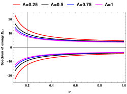
(a)

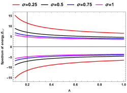
(b)

Figure 1: Energy spectrum with $\sigma$ and $\Lambda$. Here $\ell=1,k=1,M=1$.

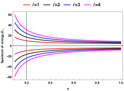
(a)

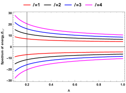
(b)

Figure 2: Energy spectrum with $\sigma$ and $\Lambda$ for different quantum numbers $\ell$. Here $k=1,M=1$.

2.2 Cornell-type potential

In this part, we consider a linear plus Coulomb-type potential together called Cornell-type potential given by

$$S=\eta\,\rho+\frac{\xi}{\rho},$$ (33)

where $\xi>0$ is potential parameter. The linear part is responsible for long range interactions whereas the Coulomb part for short range interactions. The Cornell potential consists of a linear potential plus a Coulomb potential and a harmonic term that is used in quark-antiquark interaction [59]. This type of potential has widely been used in the studies of quantum mechanical system by numerous authors (see, refs. [56, 54, 44]. Thereby, substituting this Cornell-type potential into the radial equation (10) and considering first order approximation reduces to the following differential equation form:

$$\psi^{\prime\prime}+\frac{1}{\rho}\,\psi^{\prime}+\Bigg{[}\beta^{2}-2\,\eta\,\xi-2\,M\,\eta\,\rho-\eta^{2}\,\rho^{2}-\frac{2\,M\,\xi}{\rho}-\frac{\iota^{2}}{\rho^{2}}\Bigg{]}\,\psi=0,$$ (34)

where

$$\iota^{2}=\xi^{2}+\tau^{2}=\xi^{2}+\frac{\ell^{2}/\sigma^{2}}{2\,\Lambda}.$$ (35)

Analogue to the previous section, let us consider the following wave function ansatz:

$$\psi\left(\rho\right)=\rho^{\left|\iota\right|}\mathrm{e}^{-\frac{1}{2}\rho^{2}\eta-M\rho}\Omega(\rho)$$ (36)

Substituting this wave function into the equation (34) results the following differential equation form:

$$\Omega^{\prime\prime}+\left[-2\,M-2\,\eta\,\rho+\frac{(2\,\iota+1)}{\rho}\right]\,\Omega^{\prime}+\left[M^{2}+\beta^{2}-2\,\xi\,\eta-2\,(1+\iota)\,\eta-\frac{2\,M}{\rho}\left(\xi+\iota+\frac{1}{2}\right)\right]\,\Omega=0.$$ (37)

Transforming to a new variable via the following transformation $\mathcal{P}=\sqrt{\eta}\rho$ into the above differential equation results

$$\Omega^{\prime\prime}+\left[\frac{2\,\iota+1}{\mathcal{P}}-\frac{2\,M}{\sqrt{\eta}}-2\,\mathcal{P}\right]\Omega^{\prime}+\left[\frac{M^{2}+\beta^{2}-2\,\xi\,\eta}{\eta}-2\,(\iota+1)-\frac{\left(\frac{M}{\sqrt{\eta}}\right)}{\mathcal{P}}\,(2\,\xi+2\,\iota+1)\right]\,\Omega=0.$$ (38)

Defining the following parameters

$$\delta=\frac{2M}{\sqrt{\eta}},\quad\gamma=\frac{M^{2}+\beta^{2}-2\,\xi\,\eta}{\eta}-2\,(\iota+1),\quad\varsigma=\frac{M}{\sqrt{\eta}}(2\,\xi+2\,\iota+1)$$ (39)

into the equation (38), we obtain the following standard differential equation form given by

$$\mathcal{P}\,\Omega^{\prime\prime}+\left(1+2\,\iota-\delta\,\mathcal{P}-2\,\mathcal{P}^{2}\right)\,\Omega^{\prime}+\left(\gamma\,\mathcal{P}-\varsigma\right)\,\Omega=0.$$ (40)

This differential equation is the Biconfluent Heun equation form [57] whose solution is given by

$$\Omega\left(\mathcal{P}\right)=\mathrm{HeunB}\left(2\,\iota,\delta,\gamma+2\,(\iota+1),2\,\varsigma-4\,(\iota+1),\mathcal{P}\right).$$ (41)

Following the previous analysis, we choose a power series given by [58]

$$\Omega\left(\mathcal{P}\right)=\sum_{j=0}^{\infty}\mathcal{D}_{j}\mathcal{P}^{j}$$ (42)

into the differential equation (40), we get the following coefficient

$$\mathcal{D}_{1}=\frac{\varsigma}{\left[(2\,\iota+1)\right]}\,\mathcal{D}_{0}$$ (43)

with the three-terms recurrence relation given by

$$\mathcal{D}_{j+2}=\frac{\left[\alpha^{\prime}\,(j+1)+\varsigma\right]}{\left[\left(j+2\right)\left(2\left|\iota\right|+j+2\right)\right]}\mathcal{D}_{j+1}+\frac{\left[2j-\gamma\right]}{\left[\left(j+2\right)\left(2\left|\iota\right|+j+2\right)\right]}\mathcal{D}_{j}$$ (44)

The truncating conditions of the power series are given by

$$\mathcal{D}_{j+1}=0,\quad\gamma=2\,j$$ (45)

Simplification of the second condition gives the following expression of the energy eigenvalues

$$E_{j,\ell}=\pm\,\sqrt{k^{2}+2\,\eta\,\Bigg{(}j+1+\xi+\sqrt{\xi^{2}+\frac{\ell^{2}}{2\,\Lambda\,\sigma^{2}}}\Bigg{)}}.$$ (46)

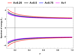
(a)

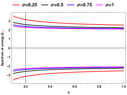
(b)

Figure 3: Energy spectrum with $\sigma$ and $\Lambda$. Here $\xi=\eta=0.5,j=1,k=1,M=1$

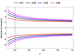
(a)

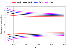
(b)

Figure 4: Energy spectrum with $\sigma$ and $\Lambda$ for different quantum number $\ell$. Here, $\xi=\eta=0.5,j=1,k=1,M=1$

The corresponding wave function is given by

$$\psi_{j,\ell}=\mathcal{N}_{2}\,\rho^{\iota}\,\mathrm{e}^{-\frac{1}{2}\,\rho^{2}\,\eta-M\,\rho}\,\mathrm{HeunB}\left(2\,\iota,\frac{2\,M}{\sqrt{\eta}},\frac{M^{2}+\beta^{2}-2\,\eta\,\xi}{\eta},\frac{4\,M\,\xi}{\sqrt{\eta}},\sqrt{\eta}\,\rho\right).$$ (47)

The ground-state of the quantum system is defined by $j=1$. Therefore, from (45) we have $\mathcal{D}_{2}=0$ and $\gamma=2$. But from the recurrence relation (44), we obtain by setting $\mathcal{D}_{2}=0$ as follows:

$$\mathcal{D}_{1}=\frac{2}{\varsigma+\alpha^{\prime}}\,\mathcal{D}_{0}.$$ (48)

Equating equations (43) and (48) and simplification results

$$\eta_{1,\ell}=\frac{M^{2}}{\Big{(}\frac{1}{2}+\sqrt{\xi^{2}+\frac{\ell^{2}}{2\,\Lambda\,\sigma^{2}}}\Big{)}}\,\Bigg{(}\xi+\frac{1}{2}+\sqrt{\xi^{2}+\frac{\ell^{2}}{2\,\Lambda\,\sigma^{2}}}\Bigg{)}\,\Bigg{(}\xi+\frac{3}{2}+\sqrt{\xi^{2}+\frac{\ell^{2}}{2\,\Lambda\,\sigma^{2}}}\Bigg{)}.$$ (49)

a constraint on the potential parameter $\eta$ that gives us allowed values of the energy level and a first order polynomial of $\Omega$.

Therefore, the ground state energy level is given by

$$E_{1,\ell} = \pm\,\Bigg{[}k^{2}+\frac{2\,M^{2}}{\Bigg{(}\frac{1}{2}+\sqrt{\xi^{2}+\frac{\ell^{2}}{2\,\Lambda\,\sigma^{2}}}\Bigg{)}}\,\Bigg{(}\xi+\frac{1}{2}+\sqrt{\xi^{2}+\frac{\ell^{2}}{2\,\Lambda\,\sigma^{2}}}\Bigg{)}\,\Bigg{(}\xi+\frac{3}{2}+\sqrt{\xi^{2}+\frac{\ell^{2}}{2\,\Lambda\,\sigma^{2}}}\Bigg{)}\times$$ (50)

$$\,\Bigg{(}2+\xi+\sqrt{\xi^{2}+\frac{\ell^{2}}{2\,\Lambda\,\sigma^{2}}}\Bigg{)}\Bigg{]}^{1/2}.$$

The corresponding ground-state wave function is given by

$$\psi_{1,\ell}=\rho^{\iota}\,\mathrm{e}^{-\frac{1}{2}\,\rho^{2}\,\eta_{1,\ell}-M\,\rho}\,\Big{[}\mathcal{D}_{0}+\mathcal{D}_{1}\,\sqrt{\eta}\,\rho\Big{]},$$ (51)

where

$$\mathcal{D}_{1}=\sqrt{\frac{\Bigg{(}\xi+\frac{1}{2}+\sqrt{\xi^{2}+\frac{\ell^{2}}{2\,\Lambda\,\sigma^{2}}}\Bigg{)}}{\Bigg{(}\frac{1}{2}+\sqrt{\xi^{2}+\frac{\ell^{2}}{2\,\Lambda\,\sigma^{2}}}\Bigg{)}\,\Bigg{(}\xi+\frac{3}{2}+\sqrt{\xi^{2}+\frac{\ell^{2}}{2\,\Lambda\,\sigma^{2}}}\Bigg{)}}}.$$ (52)

Equation (50) is the relativistic ground state energy level and equations (51)–(52) is the corresponding ground state wave function of a relativistic scalar particle in the background of Bonnor-Melvin magnetic universe in the presence of a Cornell-type scalar potential. Following the similar procedure, we one find excited states energy levels and the wave function of the quantum system defined by the mode $j\geq 2$. We see that the ground-state energy spectrum and the wave function is influenced by the topology parameter $\sigma$ of the geometry, the cosmological constant $\Lambda$ and the potential parameter $\xi$ related with Coulomb-type potential. We also see that the ground-state energy level $E_{1,\ell}$ for scalar particle-antiparticles are equally spaced on either side about $E=0$ for a fixed quantum number $\ell$ and potential values $\xi$.

3 Conclusions

We conducted an investigation into the relativistic quantum dynamics of scalar particles within the background of a magnetic universe, taking into consideration the presence of a cosmological constant. Our focus was on the Bonnor-Melvin magnetic universe, wherein the strength of the magnetic field is contingent upon the topological parameter $\sigma$ and the cosmological constant $\Lambda$. Additionally, we introduced a static non-electromagnetic scalar potential denoted as $S$, modifying the mass term $M\to(M+S)$ within the Klein-Gordon equation. We derived the radial wave equation for this scalar potential in the magnetic universe background. Specifically, we opted for a linear confining potential and solved the resulting radial equation, which took the form of a Biconfluent Heun second-order differential equation. Employing a power series solution method, we obtained eigenvalue solution, for example, the ground state energy level and the corresponding wave function for the scalar particles. Notably, we demonstrated that the eigenvalue solution is influenced by the topology of the geometry represented by $\sigma$ and the cosmological constant $\Lambda$, resulting in modifications. Subsequently, we selected a Cornell-type scalar potential, and following the established procedure, we presented the ground state energy level and the radial wave function. In this case, we observed that the eigenvalue solution is not only influenced by the previously mentioned parameters $\sigma$ and $\Lambda$ but also by the potential parameter $\xi$.

We have generated several figures illustrating the energy spectrum (31) and (50) in relation to the topology parameter $\sigma$ and the cosmological constant $\Lambda$. In Figure 1(a), we observe that as the values of the cosmological constant $\Lambda$ increase while keeping $\ell=1=k=M$ constant, the energy levels decrease, shifting downward with increasing values of the parameter $\sigma$. A similar trend is also evident in Figure 1(b) as the values of the topology parameter $\sigma$ increase. In Figure 2(a), for a fixed cosmological constant value of $\Lambda=0.5$, the decreasing energy levels shift upward with an increase in the quantum number $\ell$. A parallel observation can be made in Figure 2(b) for a fixed value of $\sigma=0.5$. The trends depicted in Figures 3 and 4 can be explained in a similar manner.

Certainly, we have explored a fascinating subject, focusing into the relativistic dynamics of scalar fields in the presence of non-electromagnetic potentials within the framework of a magnetic universe. It is noteworthy that the eigenvalue solutions are modified not only by the topological characteristics of the geometry but also by the cosmological constant, along with the inherent potential parameters. This investigation sheds light on the interplay of factors influencing the quantum behavior of scalar fields in a gravitational context. It is essential to highlight that the link between gravity theory and quantum mechanics remains elusive and not fully understood. The intricacies of how gravitational fields interact with quantum particles, especially in the presence of non-electromagnetic potentials, present a rich area for further exploration and research.

Conflict of Interest

There is no conflict of interests in this paper.

Funding Statement

There is no funding agency associated with this manuscript.

Data Availability Statement

No new data are generated or analysed during this study.

References

- [1] A. Einstein, Annalen Phys. 49, 769 (1916).
- [2] B. P. Abbott et al, Phys Rev Lett 116, 061102 (2016).
- [3] K. Akiyama et al, Astrophys J Lett 875, L1 (2019).
- [4] R. P. Feynman, and A. R. Hibbs, Quantum mechanics and path integrals, Courier Corporation(1965).
- [5] M. D. Schwartz, Quantum field theory and the standard model, Cambridge University Press (2013).
- [6] A. Ashtekar, and J. J. Stachel, Conceptual problems of quantum gravity, Birkhäuser (1991).
- [7] L. Smolin, The trouble with physics: The rise of string theory, the fall of a science, and what comes next, Mariner Books (2007).
- [8] L. I. Schiff, Phys. Rev. Lett.4,215(1960).
- [9] J. Lense and H. Thirring, Physikalische Zeitschrift, 19,156(1918).
- [10] B. P. Abbot et al., Phys. Rev. Lett., 116, 6(2016).
- [11] A. Einstein, Science, 84, 506–507 (1936).
- [12] S. Refsdal and J. Surdej, Reports on Progress in Physics, 57,117 (1994).
- [13] C. Thompson and R. C. Duncan, Monthly Notices of the Royal Astronomical Society, 275, 255 (1995).
- [14] C. Kouveliotou et al., Nature, 393, 235 (1998).
- [15] U. Gürsoy, D. Kharzeev, and K. Rajagopal, Phys. Rev. C, 89, 054905 (2014).
- [16] A. Bzdak and V. Skokov, Physics Letters B, 710, 171 (2012).
- [17] V. Voronyuk, V. D. Toneev, W. Cassing, E. L. Bratkovskaya, V. P. Konchakovski, and S. A. Voloshin, Phys. Rev. C, 83, 054911 (2011).
- [18] T. Gutsunaev and V. Manko, Phys. Lett. A 123, 215 (1987).
- [19] T. Gutsunaev and V. Manko, Phys. Lett. A 132, 85 (1988).
- [20] W. B. Bonnor, Proc. Phys. Soc. Section A 67, 225 (1954).
- [21] M. Melvin, Phys. Lett. 8, 65 (1964).
- [22] M. Žofka, Phys. Rev. D 99, 044058 (2019).
- [23] L. Parker, Phys. Rev. Lett. 44, 1559 (1980).
- [24] N. D. Birrell, N. D. Birrell, and P. Davies, Quantum fields in curved space,” Cambridge University Press (1984).
- [25] E. Elizalde, Phys. Rev. D 36, 1269 (1987).
- [26] S. Chandrasekhar, Proc. Roy. Soc. London. A. Math. Phys. Sci. 349, 571 (1976).
- [27] L. C. N. Santos and C. C. Barros Jr., Eur. Phys. J. C 77, 186 (2017).
- [28] L. C. N. Santos and C. C. Barros Jr., Eur. Phys. J. C 78, 13 (2018).
- [29] R. L. L. Vitória and K. Bakke, Eur. Phys. J. C 78, 175 (2018).
- [30] F. Ahmed, Int. J. Mod. Phys. A 37, 2250186 (2022).
- [31] F. Ahmed, Commun. Theor. Phys. 75, 025202 (2023).
- [32] L. C. N. Santos, C. E. Mota, and C. C. Barros Jr., Adv. High Energy Phys. 2019, 2729352 (2019).
- [33] Y. Yang, Z.-W. Long, Q.-K. Ran, H. Chen, Z.-L. Zhao, and C.-Y. Long, Int. J. Mod. Phys. A 36, 2150023 (2021).
- [34] A. R. Soares, R. L. L. Vitória, and H. Aounallah, Eur. Phys. J. Plus 136, 966 (2021).
- [35] A. Bouzenada, A. Boumali, Ann. Phys. 452, 169302 (2023).
- [36] A. Bouzenada, A. Boumali, R. L. L. Vitoria, F. Ahmed and M. Al-Raeei, Nucl. Phys. B 994, 116288 (2023).
- [37] A. Bouzenada, A. Boumali and F. Serdouk, Theor. Math. Phys,216, 1055 (2023).
- [38] A. Bouzenada, A. Boumali, and E. O. Silva, Ann. Phys. 458, 169479 (2023).
- [39] V. B. Bezerra, M. S. Cunha, L. F. F. Freitas, C. R. Muniz, and M. O. Tahim, Mod. Phys. Lett. A 32, 1750005 (2016).
- [40] L. C. N. Santos and C. C. Barros Jr., Int. J. Mod. Phys. A 33, 1850122 (2018).
- [41] E. O. Pinho and C. C. Barros Jr., Eur. Phys. J. C. 83, 745 (2023).
- [42] P. Sedaghatnia, H. Hassanabadi, and F. Ahmed, Eur. Phys. J. C. 79, 541 (2019).
- [43] cA. Guvendi, S. Zare and H. Hassanabadi, Phys. Dark Univ. 38, 101133 (2022).
- [44] R. L. L. Vitória and K. Bakke, Eur. Phys. J. Plus 133, 490 (2018).
- [45] L. C. N. Santos and C. C. Barros Jr., Eur. Phys. J. C 76, 560 (2016).
- [46] O. Klein, Z. Phys 37, 895 (1926).
- [47] W. Gordon, Z. Phys 40, 117 (1926).
- [48] A. Boumali, R. Allouani , A. Bouzenada, and F. Serdouk. Ukr. J. Phys. 68, 235 (2023).
- [49] H. Hassanabadi, S. Zare and Marc de Montigny, Gen. Relativ. Gravit. 50, 104 (2018).
- [50] L. G. Barbosa, and C. C. Barros Jr, arXiv:2311.11148 [gr-qc].
- [51] L. G. Barbosa, and C. C. Barros Jr, arXiv:2310.04883 [gr-qc].
- [52] W. Greiner, Relativistic Quantum Mechanics. Wave Equations, Springer-Verlag, Berlin, Gemnay (2000).
- [53] C. L. Chrichfield, J. Math. Phys. 17, 261 (1976).
- [54] E. R. F. Medeiros and E. R. B. de Mello, Eur. Phys. J C 72, 2051 (2012).
- [55] F. Ahmed, Eur. Phys. J. C 79, 104 (2019).
- [56] Z. Wang, Z. Long, C. Long, and M. Wu, Eur. Phys. J Plus 130, 36 (2015).
- [57] A. Ronveaux, Heun’s Differential Equations, A Clarendon Press Publication (1995).
- [58] G. B. Arfken, H. J. Weber and F. E. Harris Mathematical Methods for Physicists, Elsevier, Academic Press (2012).
- [59] M. K. Bahar and F. Yasuk, Adv. High Energy Phys. 2013, 814985 (2013).