Information theory for model reduction in stochastic dynamical systems

Abstract

Model reduction is the construction of simple yet predictive descriptions of the dynamics of many-body systems in terms of a few relevant variables. A prerequisite to model reduction is the identification of these relevant variables, a task for which no general method exists.Here, we develop a systematic approach based on the information bottleneck to identify the relevant variables, defined as those most predictive of the future. We elucidate analytically the relation between these relevant variables and the eigenfunctions of the transfer operator describing the dynamics. Further, we show that in the limit of high compression, the relevant variables are directly determined by the slowest-decaying eigenfunctions. Our information-based approach indicates when to optimally stop increasing the complexity of the reduced model. Further, it provides a firm foundation to construct interpretable deep learning tools that perform model reduction. We illustrate how these tools work on benchmark dynamical systems and deploy them on uncurated datasets, such as satellite movies of atmospheric flows downloaded directly from YouTube.

I Introduction

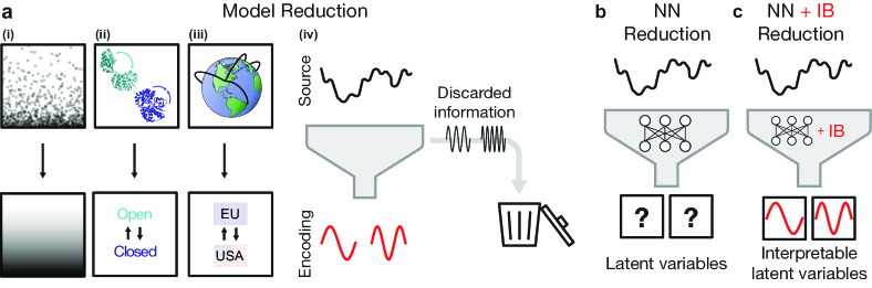
Figure 1: Interpretable dynamical variables in reduced models via the information bottleneck. (a) Model reduction. (a.i) The long time dynamics of particles in a box can be compressed into a continuous scalar field. (a.ii) An enzyme (here, inorganic pyrophosphatase) which undergoes a large conformational change can be described by the locations of all its constituent atoms, or by a simple binary variable representing whether it is open or closed. (a.iii) People or goods which flow between geographical locations can be reduced into a simpler model representing, for example, total flow between countries. (a.iv) The information bottleneck performs model reduction by finding a lossy compression of a signal into a simpler discrete or continuous variable predictive of the future state. (b) Neural networks, in particular those with autoencoder-type architectures, can compress inputs into a reduced latent representation which are not interpretable a priori. (c) By combining these with an IB loss function, the latent variables can be interpreted as eigenfunctions of the system’s transfer operator, i.e. the slowest-varying functions under the dynamics.

The exhaustive description of a physical system is usually impractical due to the sheer volume of information involved. As an example, the air in your office may be described by a $10^{27}$–dimensional state vector containing the positions and momenta of every particle in the room. Yet, for most practical purposes, it can be effectively described using only a small number of quantities such as pressure and temperature. Similar reductions can be achieved for physical systems ranging from diffusing particles to biochemical molecules and complex networks (Fig. 1a). In all cases, certain “relevant variables” can be predicted far into the future even though individual degrees of freedom in the system are effectively unpredictable.

The process by which one goes from the complete description of a system to a simpler one is known as model reduction. Several procedures for model reduction exist across the natural sciences. They range from analytical methods, such as adiabatic elimination and multiple-scale analysis [1, 2, 3, 4, 5, 6, 7, 8, 9, 10], to data-driven methods such as dynamic mode decomposition, diffusion maps, and spectral submanifolds [11, 12, 13, 14, 12, 15, 16, 17, 18, 19, 20, 21, 22].

The success of these approaches is limited by a fundamental difficulty: before performing any reduction, one has to identify a decomposition of the full system into relevant and irrelevant variables. In the absence of physical intuition (e.g. a clear separation of scales), identifying such a decomposition is an open problem [4]. It may not even be clear a priori when to stop increasing the complexity of a simplified model or, conversely, when to stop reducing the amount of information needed to represent the dynamical state of a many body system. In both cases, one must first determine the minimal number of relevant variables that are needed. The answer to this question depends in fact on how precisely and how far in the future you wish to forecast. Nonetheless, this answer should be compatible with fundamental constraints on forecasting set by external perturbation and finite measurement accuracy [23].

In order to address the difficulty identified in the previous paragraph, we develop an information-theoretic framework for model reduction. Very much like MP3 compression is about retaining information that matters most to the human ear [24], model reduction is about keeping information that matters most to predict the future [25]. Inspired by this simple insight, we formalize model reduction as a lossy compression problem known as the information bottleneck (IB) [26, 27, 28]. This formal step allows us to give a precise answer to the question of how to identify relevant and irrelevant variables. We show how and under what conditions the standard operator-theoretic formalism of dynamical systems [29, 19], which underlies most methods of model reduction, naturally emerges from optimal compression. Crucially, our framework systematically answers the question of when to stop increasing the complexity of a minimal model (or reducing the information needed to represent a many body state). Further, it provides a firm foundation to address a practical problem: the construction of deep learning tools to perform model reduction that are guaranteed to be interpretable (Fig. 1b-c). We illustrate our approach on benchmark dynamical systems and demonstrate that it works even on uncurated datasets, such as satellite movies of atmospheric flows downloaded directly from YouTube.

The remainder of this paper is structured as follows. In Section II, we provide an introduction to the information-theoretic background needed to formulate the IB problem. Next, we prove that the most informative features identified by IB correspond to the eigenfunctions of the transfer operator describing the time evolution of a noisy dynamical system (via its probability distribution). In Section III, we relate the spectrum of the transfer operator with the rate at which noisy dynamical systems loose information about their initial state. In Section IV, we show that mutual information can be used as a metric for the fidelity of discrete reduced models which tells us “when to stop” increasing the complexity of the model [23]. The level of noise in the system critically impacts this stopping criterion. In Section V, we numerically solve the exact IB optimization problem in the limit of high compression, confirming our analytical results. In Section VI, we turn to deep learning methods to find approximate solutions to the IB problem. To do so, we use a variational formulation of IB where the relevant variables in the reduced model are learned as latent variables in a neural network [30]. The learned variables in these networks are naturally interpretable as transfer operator eigenfunctions. We demonstrate this feature on benchmark dynamical systems: the Hopf oscillator, the Lorenz-63 system [31], and Navier-Stokes equations. In Section VII, we apply our method on uncurated experimental datasets such as videos of von Kármán streets obtained in the laboratory as well as from satellite-based observations of the Earth’s atmosphere.

II Model reduction as a compression problem

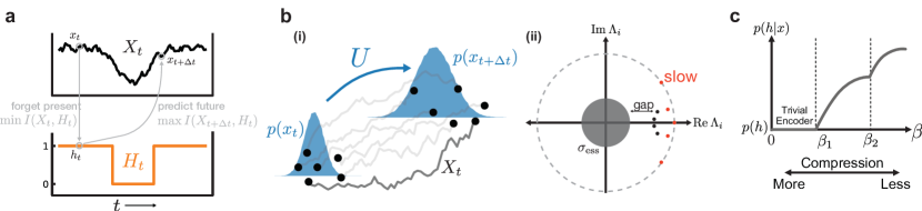
Figure 2: Dynamical system compression via information bottleneck and transfer operators. (a) The information bottleneck for dynamical systems aims to reduce the state $x$ into a lower-dimensional (here, discrete) variable $h$ by forgetting as much as possible about the current time, yet retaining predictive power about the future $x_{t+\Delta t}$. (b.i) We consider systems that evolve according to a linear transfer operator $U$, which acts on probability distributions. (b.ii) The point spectrum of $U$ contains several slowly decaying modes (red). We assume that the essential spectrum $\sigma_{\text{ess}}$ has a small spectral radius relative to the point spectrum. (c) Schematic evolution of the encoder $p(h|x)$ for varying $\beta$. For low $\beta$ (high compression), the encoder is trivial. After the first IB transition at $\beta_{1}$, the encoder becomes non-trivial by gaining some dependence on $x$.

Any system in the real world is subject to measurement noise or random fluctuations or both. We therefore describe dynamical systems using random variables: let $p_{X_{t}}(x)$ be the probability of finding a system in a state $x\in\mathcal{M}$ at time $t$, where $\mathcal{M}$ is the space of all possible states of the system ($X_{t}$ denotes the corresponding random variable). Deterministic systems are naturally encompassed in this description by taking all probabilities to be either 0 or 1. We wish to identify a reduced description of the system in terms of so-called relevant variables $h$ ($H_{t}$ is the corresponding random variable). A reduction of $x$ into $h$ can be understood as a probabilistic encoding $p_{H_{t}|X_{t}}(h|x)$ which gives the probability of attributing the value $h$ to the state $x$. In the following, we use shorthands such as $p(h|x)$ for $p_{H_{t}|X_{t}}(h|x)$ when the meaning is clear.

For $p(h|x)$ to be a useful and efficient reduction, the resulting variable $h$ should contain just enough information to predict the state of the system in the future. This objective can be formalized in the so-called information bottleneck (IB) framework [26]. Formally, an encoder $p(h|x)$ is sought which minimizes the IB Lagrangian

$$\mathcal{L}_{\text{IB}}[p(h_{t}|x_{t})] =I(X_{t},H_{t})-\beta I(X_{t+\Delta t},H_{t})$$ (1)

with the mutual information for two random variables $X$ and $Y$ given by

$$I(X,Y) =\int\text{d}x\,\text{d}y\,p(y|x)p(x)\log\frac{p(y|x)}{p(y)}$$ (2)

$$=S(Y)-S(Y|X)$$ (3)

where $S(X)=-\int p(x)\log p(x)$ is the entropy of $X$.

The optimal encoder

$$p_{\beta}^{*}(h|x)=\text{arg min}\;\mathcal{L}_{\text{IB}}$$ (4)

compresses as much information as possible about the current state $x_{t}$, while maximizing the information retained about the future state $x_{t+\Delta t}$ (Fig. 2a) [27]. This trade-off is controlled by the parameter $\beta$. For small $\beta$ the compression term dominates and the optimal encoder is trivial, losing all information about the system. In the limit of large $\beta$ the second term dominates. In this scenario, corresponding to vanishing compression regime, the variable $H_{t}$ simply copies $X_{t}$ (or is a bijection thereof). For intermediate $\beta$ the compression term does not allow $X_{t}$ to be completely captured by $H_{t}$ so that features of $X_{t}$ must “compete” to pass through to the encoding variable.

We wish to connect the features learned by IB to the dynamical properties of $X_{t}$. We assume that the evolution in time of the system can be described by a transfer operator $U$ as (Fig. 2b.i)

$$p_{X_{t+\Delta t}}(x)=[Up_{X_{t}}](x).$$ (5)

As detailed in Appendix B, this description includes deterministic dynamical systems (for which $U$ is known as the Perron-Frobenius operator) as well as stochastic differential equations. The transfer operator $U$ can be decomposed into its right and left eigenvectors as

$$U=\sum_{n}\ket{\rho_{n}}\text{e}^{\lambda_{n}\Delta t}\bra{\phi_{n}}+U_{\text{ess}}$$ (6)

where $\rho_{n}$ are right eigenvectors with eigenvalue $\Lambda_{n}\equiv\text{e}^{\lambda_{n}\Delta t}$ and $\phi_{n}$ are the corresponding left eigenvectors ($\lambda_{n}$ are the eigenvalues of the infinitesimal generator of $U$). The operator $U_{\text{ess}}$ corresponds to the so-called essential spectrum, and we assume that it can be neglected  (Fig. 2b.ii). This is usually possible when the system is subjected to even a small amount of noise, or when some amount of uncertainty is present in the measurements [33, 34].

Our key observation is that the optimal encoder in Eq. (4) can be expressed in terms of the eigenvalues $\lambda_{n}$ and left eigenfunctions $\phi_{n}$ of (the generator of) $U$,

$$\!\!p_{\beta}^{*}(h|x)=\frac{1}{\mathcal{N}(x)}\,p_{\beta}^{*}(h)\,\exp\left[\beta\sum_{n}\text{e}^{\lambda_{n}\Delta t}\phi_{n}(x)f_{n}(h)\right]$$ (7)

where $f_{n}(h)$ are factors that do not depend on $x$ (cf. Appendix C). These factors effectively parameterize the encoder’s dependence on $x$ by weighting the respective eigenfunctions $\phi_{n}$. Equation (7) is valid for arbitrary $\beta$. When $\beta$ is small so that the encoder is trivial, the value $h$ is assigned at random with no regard to the state $x$ of the system. The trivial encoder satisfies $p(h|x)=p(h)$ so that the factors $f_{n}$ are all equal to zero. As $\beta$ is increased, the encoder undergoes a series of transitions at $\beta=\beta_{1}<\beta_{2}<\beta_{3}...$ where new features are allowed to pass through the bottleneck (Fig. 2c) [35, 36, 37, 38]. The first transition happens at a finite value of $\beta_{1}$ when the first most predictive feature is learnt. This transition represents a perturbation around the trivial encoder where the coefficients $f_{n}$ become non-zero.

Surprisingly, we find that at the first IB transition the vector of $f_{n}$ coefficients is dominated by a single term $f_{1}$. This tells us that for high compression, the most relevant feature is the subleading eigenfunction $\phi_{1}(x)$. We understand this observation by performing a perturbative expansion of the IB objective for small $f_{n}$ at the first transition. Concretely, we consider a transfer operator $U$ with infinitesimal generator $\mathcal{L}_{U}$. For $\mathcal{L}_{U}$ with a discrete spectrum with eigenvalues satisfying $0=\lambda_{0}>\lambda_{1}>\lambda_{2}\gg\lambda_{3}...$ and for $\beta$ just above the first IB transition $\beta_{1}$, we can show that the optimal encoder is given approximately by

$$p^{*}_{\beta}(h|x)=\frac{1}{\mathcal{N}(x)}p^{*}_{\beta}(h)\,\exp\left(\beta\,\text{e}^{\lambda_{1}\Delta t}\phi_{1}(x)f_{1}(h)\right)$$ (8)

with corrections due to the second eigenfunction given by $f_{2}(h)\approx f_{1}(h)\text{e}^{-\Gamma\Delta t}+\mathcal{O}(\text{e}^{-2\Gamma\Delta t})$ where $\Gamma=\lambda_{1}-\lambda_{2}>0$ denotes the spectral gap. A proof of Eq. 8 subject to some further technical assumptions may be found in Appendix C.

The above statement shows that in the limit of high compression the encoder’s dependence on $x$ is given by the first left eigenfunction $\phi_{1}(x)$, which is the slowest-varying function of the state under dynamics given by $U$. Therefore, Eq. 8 makes precise the intuitive statement that slow features are the most relevant for predicting the future. Our analytical result, while applying only to the dominant eigenfunction, is valid for arbitrary non-Gaussian variables. The question of maximally informative features has additionally been explored in the context of animal vision, where one seeks to understand what features of the field of vision are encoded by retinal neurons [39, 40].

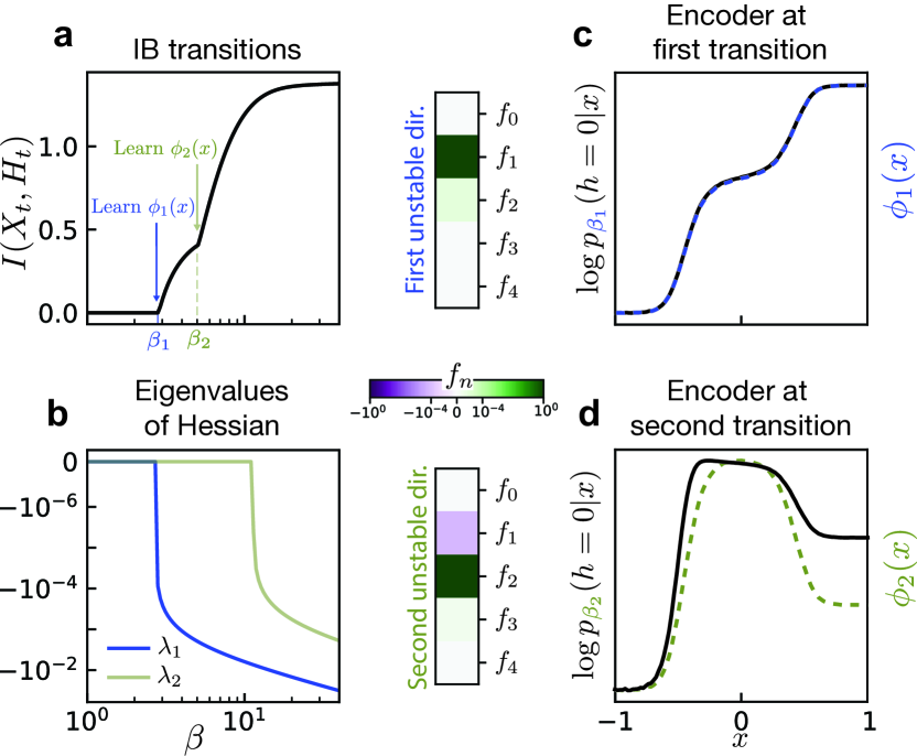
Figure S1: IB transitions for a Brownian particle in a triple-well potential. (a) Information transitions with varying $\beta$ for a particle in a triple-well potential. (b) Eigenvalues of the IB Hessian evaluated at the uniform encoder $p(h|x)=N_{H}^{-1}$. The appearance of an unstable direction at $\beta_{1}\approx 3$ coincides with the first IB transition. The emergence of a second unstable direction doesn’t correspond precisely to the IB transition at $\beta_{2}$ because stability is evaluated at the uniform encoder, but the true optimal encoder at $\beta_{2}$ is not uniform. (c) The unstable directions are dominated by single components (note the color scale is logarithmic). At the first transition, the logarithm of the encoder is given by the eigenfunction $\phi_{1}(x)$, up to rescaling ($y$-axis is shown in arbitrary units). (d) Likewise, at the second transition the encoder is given primarily by $\phi_{2}(x)$.

We further observe numerically that this picture holds true more generally: also at successive IB transitions, the learned features correspond to successive modes of the transfer operator (Fig. S1). This picture is consistent with the exact results known for Gaussian IB, where the encoder learns eigenvectors of a matrix (related to the covariance of the joint $X_{t},X_{t+\Delta t}$ distribution) in a step-wise fashion at each IB transition [37]. Together, this shows that the most informative features extracted by IB, an agnostic information-theoretic approach, correspond to physically-interpretable quantities – namely transfer operator eigenfunctions.

III Information decay and the spectrum of the transfer operator

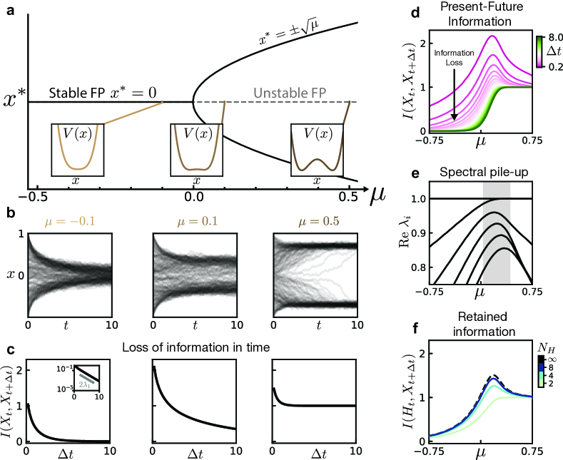
Figure 3: Information loss of a Brownian particle in a double well potential. (a) Fixed point (FP) diagram of the dynamics given by Eq. 9 for zero noise. There is a bifurcation at $\mu=0$ where the stable FP at $x=0$ becomes unstable and two new stable FPs appear at $\pm\sqrt{\mu}$. Insets show the evolution of the corresponding potential $V(x)$, with the emergence of a double-well structure for $\mu>0$. (b) Dynamics of the system Eq. 9 for varying values of $\mu$ corresponding to the potential insets in (a), with uniformly-distributed initial conditions. (c) Loss of information between the initial condition and the future state. Inset shows scaling given by the first eigenvalue of the transfer operator. (d) Mutual information between the present and future state for varying time delay $\Delta t$ and bifurcation parameter $\mu$. (e) Spectrum of the transfer operator $U$, showing a pile-up of eigenvalues for $\mu\gtrsim 0$. These are related to the eigenvalues of its infinitesimal generator by $\Lambda_{i}=\text{e}^{\lambda_{i}\Delta t}$. (f) Maximal mutual information which can be encoded into a discrete variable of $N_{H}$ values, for a fixed time delay $\Delta t=1.0$. Black dashed line shows $I(X_{t},X_{t+\Delta t})$ for reference.

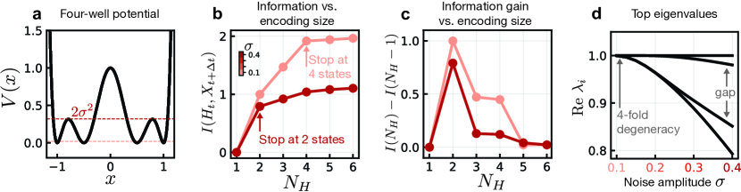
Figure 4: “Knowing when to stop”. The spectral properties of the transfer operator determine the necessary complexity (i.e. “when to stop” [23]) of the reduced model, which we show is also visible in information theoretic metrics. (a) Four-well potential in which a Brownian particle fluctuates. The magnitude $\sigma$ of the fluctuating noise is related to an energy scale $E_{\sigma}\sim 2\sigma^{2}$. (b) Information contained in the encoding variable $H_{t}$ about the future state $X_{t+\Delta t}$ for varying levels of noise and alphabet sizes $N_{H}$. (c) Information gain achieved by increasing the alphabet size by a single variable. This is the discrete derivative of the curve in (b). (d) Spectrum of the transfer operator for changing values of noise amplitude.

To develop intuition for information in a dynamical system and the information bottleneck encoder, we turn to a simple system which describes a Brownian particle trapped in a confining double-well potential. This might represent, for example, a molecule with a single degree of freedom that transitions between two metastable configurations [41]. In the overdamped limit the state of the particle is completely determined by its position $X_{t}\in\mathbb{R}$, with dynamics given by the Langevin equation

$$\dot{x}_{t} =-\partial_{x}V(x_{t})+\sigma\eta_{t}.$$ (9a)

$$V(x) =\frac{1}{4}(\mu-x^{2})^{2}$$ (9b)

Here, $\eta_{t}$ is unit-variance white noise, $\sigma$ controls its strength, and $\mu$ controls the shape of the potential $V(x)$.

The deterministic dynamical system undergoes a bifurcation at $\mu=0$ (Fig. 3a). For $\mu<0$, the potential features a single well, which then becomes two for positive $\mu$ (figure insets). Sample trajectories, with noise, for a uniform initial distribution of particles are shown in Fig. 3b. For negative $\mu$, the trajectories all converge to a fixed point at $x=0$, while for $\mu>0$ they fluctuate around the fixed points at $x=\pm\sqrt{\mu}$. When $\mu$ is small but positive, the particle may occasionally transition from one potential well to the other because of thermal fluctuations.

To quantify the amount of information about the future state $X_{t+\Delta t}$ contained in the initial state $X_{t}$, we compute the mutual information between them (Fig. 3c). We estimate transition probabilities $p(x_{t+\Delta t}|x_{t})$ with an Ulam scheme where we bin trajectories by their initial and final states (see Appendix D). The dynamics of $X_{t}$ are Markovian, so that for any sequence of times $t_{0}<t_{1}<t_{2}$, $p(X_{t_{2}}|X_{t_{1}},X_{t_{0}})=p(X_{t_{2}}|X_{t_{1}})$. From the data processing inequality, one has [28]

$$I(X_{t_{2}};X_{t_{0}})\leq I(X_{t_{1}};X_{t_{0}}),$$

which implies that information can only decrease in time.

What governs the rate at which information decays? Here we can already see the role of the spectrum of the dynamics’ transfer operator. By exploiting the spectral expansion of the conditional distribution $p(x_{t+\Delta t}|x_{t})$ one finds that for long times the information decays as

$$\!\!I(X_{t};X_{t+\Delta t})=e^{2\lambda_{1}\Delta t}\langle\phi_{1}^{2}\rangle\langle\rho_{1}^{2}/\rho_{0}^{2}\rangle+\mathcal{O}(e^{(\lambda_{1}+\lambda_{2})\Delta t})$$ (10)

where expectations are taken over the steady state distribution (see Appendix E). Asymptotically, the information decay is set by the value of $\lambda_{1}$, the rate of decay of the slowest-varying function $\phi_{1}(x)$ under the dynamics of $U$. For infinite times, for any value of $\mu$ even weak noise will cause the mutual information to become zero as there is a non-zero probability of hopping between the wells, though this rate of hopping is exponentially small [33].

The loss of information in time depends on the bifurcation parameter $\mu$ as summarized in Fig. 3d. Note the peak in $I(X_{t},X_{t+\Delta t})$ for small, positive $\mu$. This corresponds to dynamics where observation of $X_{t}$ strongly informs the future state; recall that the mutual information can be written as a difference of entropies Eq. 3), which is maximized when the conditional entropy $S(X_{t+\Delta t}|X_{t})\approx 0$. In contrast, for large positive or negative $\mu$, $X_{t}$ is not as informative of $X_{t+\Delta t}$ even for small times: the initial state is quickly forgotton as the particle approaches the bottom of the single (for $\mu<0$) or double (for $\mu>0$) well.

This phenomenon is reminiscent of critical slowing down, which occurs in the noise-free system as $\mu$ passes through the bifurcation at $\mu=0$. For the deterministic dynamics, the slowing down is reflected in the spectrum as a “pile up” of eigenvalues to form a continuous spectrum [33]. In the presence of noise, although the continuous spectrum becomes discrete [33, 34] there is still a pile-up of eigenvalues characterized by several eigenvalues becoming close to 1 (Fig. 3e). This pile-up gives rise to the information peak seen in Fig. 3d. The peak is not solely due to the closing of the spectral gap $\lambda_{1}-\lambda_{2}$, but is also impacted by the subdominant eigenvalues which accumulate at $\mu\approx 0.2$ (see also Fig. S2).

IV Knowing when to stop

For discrete encoding variables $h$, the information bottleneck partitions state space and reduces the dynamics on $x$ to a discrete dynamics on $h$. Such reductions of complex systems to symbolic sequences via partitioning of state space has attracted attention for more than half a century [42, 43, 44, 45]. Several works have approached this partition problem from a dynamical systems perspective, linking “optimal” partitions to eigenfunctions of the (adjoint) transfer operator [23, 46]. In this setting, a central question (posed most explicitly by Cvitanović et al. [23]) is “when to stop”: how many states does $h$ need in order to capture statistical properties of the original dynamics?

We consider this question by finding the optimal IB encoder in the limit of low compression, $\beta\gg 1$, but fixed encoding capacity $N_{H}$ (where $H_{t}\in\{0,...,N_{H}-1\}$), i.e. the encoder is only restricted by the number of symbols it can use. Analogous setup was used in the context of Renormalization Group transformations in [47, 48, 49]. In this regime, the encoder learned by IB is deterministic; we are learning an optimal hard partition of state space. This can be seen by noting that $I(H_{t};X_{t+\Delta t})=S(H_{t})-S(H_{t}|X_{t+\Delta t})$ is maximized when the latter term is zero, which happens when $x$ unambiguously determines $h$, i.e. when $p(h|x)\in\{0,1\}$ for all $x$. The details of how the encoder is computed are discussed in the next section.

Fig. 3f shows that the number of states necessary to describe the system depends strongly on the value of $\mu$. For $|\mu|\gg 0$, a two-state discrete variable $h_{t}\in\{0,1\}$ suffices to describe the system’s future. Increasing the number of reduced variables $N_{H}$ does not allow more information to be captured. Near the information peak at $\mu\approx 0.2$ this changes: predicting the future state of the system requires a more complex hidden variable of up to $N_{H}\approx 20$ values. Above, we saw that this peak arises due to the pile-up of eigenvalues at $\mu\approx 0.2$. The content of the transfer operator spectrum is thus directly reflected in the number of encoding variables needed to capture the system’s statistics.

Noise can have a similarly dramatic impact on the reduced model complexity. Indeed, noise in some form, either inherent to the dynamics or due to measurement error, is necessary for a model to be reducible. In purely deterministic systems where the future state is a bijective function of the present state, information does not decay and complete knowledge of the state is required to predict the future.

Consider a fluctuating Brownian particle as above, where now each of the wells is split into two smaller wells, giving a total of four potential minima (Fig. 4a). As the system is in steady state, the standard deviation of the fluctuations $\sigma$ corresponds to an energy scale $E_{\sigma}=2\sigma^{2}$. For small $E_{\sigma}$, the system rarely transitions between the four potential minima. In this case, knowledge of the initial minimum is very informative of the future state of the particle. In contrast, for large fluctuations the particle can spontaneously jump between shallow minima in each large well, so that the system immediately forgets about the precise potential minimum it was in. Information about the shallow minima has been “washed out”, and only the information about the larger double-well structure remains.

To see this reflected in the information, we again consider an encoding of the initial state into a discrete variable $H_{t}\in\{0,...,N_{H}-1\}$. In both the small and large noise scenarios, a variable with $N_{H}=2$ encodes approximately one bit of information (Fig. 4b), corresponding to an $H_{t}$ which distinguishes the two large wells for $x\lessgtr 0$. For large noise this is essentially all the information that can be learned; increasing the capacity of the encoding variable beyond this provides only marginally more information about the future state (Fig. 4c). In the small noise case, the information between the encoding and the future state continues to increase to approximately two bits at $N_{H}=4$, after which it plateaus. The encoding has learned to distinguish each of the four potential wells. These observations are reflected in the transfer operator spectrum shown in Fig. 4d. For small noise, the eigenvalue $\lambda=1$ is four-fold degenerate which indicates the existence of four regions that can evolve independently under $U$, giving rise to four steady state distributions satisfying $U\rho=\rho$. These regions correspond to the potential minima. Hops between the separate minima are exceedingly rare, so that the dynamics essentially take place in the four minima independently. With larger $\sigma$ the degeneracy is lifted, resulting in one dominant subleading eigenvalue followed by a gap. The corresponding eigenfunction is one which is positive (negative) on the right (left) side of the large potential barrier at $x=0$. The only relevant piece of information is therefore which of the large wells the initial condition is contained in; all other information is lost exponentially quickly.

V Transfer operator eigenfunctions are most informative features

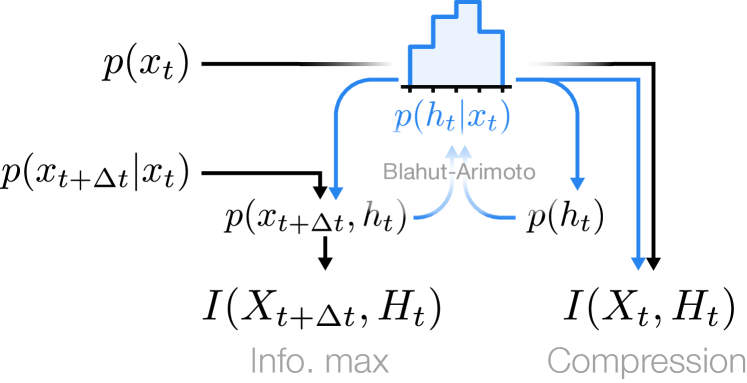
Figure 5: Exact IB. Exact IB [26] finds an optimal encoder using an iterative Blahut-Arimoto algorithm, described in the main text, for a rate-distortion problem with Kullback-Leibler distortion. This process requires access to (an estimate of) the transfer matrix and the steady state distribution. Once an optimal encoder has been found, relevant quantities such as mutual information can be computed.

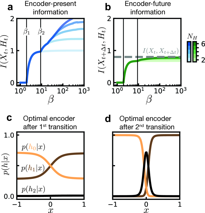
Figure 6: Information bottleneck for a Brownian particle in a double well. (a) Mutual information between the current state $X_{t}$ and its encoding $H_{t}$ for various alphabet sizes $N_{H}$ (color). The first two IB transitions are denoted with black lines and occur at $\beta_{1}$ and $\beta_{2}$. (b) Mutual information between the current state’s encoding $H_{t}$ and the future $X_{t+\Delta t}$. The gray dashed line denotes the maximum attainable information, which is the mutual information $I(X_{t},X_{t+\Delta t})$. Color denotes encoding alphabet size. Black lines showing IB transitions are shown for reference. (c) Optimal encoder after the first transition ($\beta\gtrsim\beta_{1}$) with alphabet size $N_{H}=3$. (d) Optimal encoder after the second transition ($\beta\gtrsim\beta_{2}$) with alphabet size $N_{H}=3$.

Thusfar we have concerned ourselves with encodings whose capacity is limited only by the number of variables, rather than by the compression imposed by a small value of $\beta$. In the regime of small $\beta$, or high compression, features of the state $x_{t}$ are forced to compete to make it through the bottleneck $h_{t}$. By studying the behavior of the encoder in this regime, in particular its dependence on $x_{t}$, we may identify the most relevant features of the state variable and show that they coincide with left eigenfunctions of the transfer operator.

We return to the simple example of a particle in a double well with dynamics given by Eq. (9) which we map to a discrete variable $H_{t}\in\{0,...,N_{H}-1\}$. In this system the IB loss function Eq. (1) can be optimized directly, as shown in Ref. [26], using an iterative scheme known as the Blahut-Arimoto algorithm [28]. This algorithm requires access to the exact distributions $p(x_{t})$ and $p(x_{t+\Delta t}|x_{t})$, which we approximate using an Ulam scheme (see Appendix D). After choosing some initial guess for $p(h_{t}|x_{t})$, the optimal encoder is found by iteratively computing $p(x_{t+\Delta t},h_{t})$ and $p(h_{t})$ and using these to recompute $p(h_{t}|x_{t})$.

To focus on the properties of encodings for varying degrees of compression $\beta$, we consider a fixed set of dynamical parameters $\mu$ and $\sigma$. Increasing $\beta$ reduces the amount of compression, i.e. “widens” the bottleneck, allowing more information to pass into the encoder. This leads to a series of IB transitions which are visible in $I(X_{t},H_{t})$ and $I(X_{t+\Delta t},H_{t})$ (Fig. 6a-b). The information about the present state $I(X_{t},H_{t})$ is bounded by the entropy of the random variable $X_{t}$, which occurs when $H_{t}$ exactly encodes $X_{t}$. Similarly, the information shared between the encoding state and the future $I(X_{t+\Delta t},H_{t})$ is bounded from above by $I(X_{t},X_{t+\Delta t})$: the encoding cannot contain more information about the future than the full state itself. Fig. 6b shows that $N_{H}=6$ states suffice to encode nearly all information about the future. Note that although $I(X_{t},X_{t+\Delta t})<1$ bit, two encoding variables do not suffice to encode this information.

The optimal encoder changes qualitatively at the IB transitions. Before $\beta_{1}$, the optimal encoder has no dependence on $x$ so that $p(h_{i}|x)=\text{const}$ for all $h_{i}$. After the first transition, the encoder begins to associate regions of $x$ to particular values of $h$, which can be understood as a soft partition of the state space (Fig. 6c). In this case, $h$ essentially encodes the identity of the well which the particle is currently located in. When $\beta$ is increased further, the encoder undergoes another transition and begins to distinguish states $x$ which are near the barrier of the double well (Fig. 6d).

We are interested in the form of the encoder at $\beta\gtrsim\beta_{1}$, just above the first IB transition, as this reflects the most informative features of the full state variable $x$ (Fig. 7a). The dependence of $p(h|x)$ on $x$ can be explained by our stability analysis of the IB Lagrangian performed in Appendix C. In brief, we analyze stability by considering the Hessian of the IB Lagrangian with respect to the parameters $f_{n}(h)$ in Eq. 7. These parameters tell us how much the encoder “weights” each transfer operator eigenfunction; $f_{n}(h)=0$ (for $n>0$) corresponds to the uniform encoder.

For small $\beta$ all Hessian eigenvalues $\eta_{i}$ are positive, indicating that the uniform encoder is a stable minimum of the IB Lagrangian. In Fig. 7b we show the smallest two eigenvalues of the IB Hessian Eq. 30 when evaluated at the uniform encoder $p(h|x)=p(h)$. At the first transition one eigenvalue becomes negative, so that the uniform encoder is unstable. The eigenvector corresponding to the unstable eigenvalue $\eta_{1}$ tells us how the weights $f_{n}(h)$ should be adjusted to lower the value of the IB Lagrangian. Our numerics confirm that these weights are dominated by $f_{1}$ as expected from our analytical result (Fig. 7c, top). By taking the logarithm of the encoder after the transition, we can independently confirm that the encoder depends only on $\phi_{1}(x)$ (Fig. 7d).

Our stability analysis predicts that a second mode becomes unstable at the second IB transition $\beta\approx\beta_{2}$ (Fig. 7b). Here we see that this unstable mode selects $f_{2}$, and that the encoder correspondingly gains dependence on $\phi_{2}(x)$ (Fig. 7d). Note that in general, $\eta_{2}$ must not necessarily become negative precisely at $\beta_{2}$ because the stability analysis is performed at the uniform encoder while the true optimal encoder has already deviated from uniformity. In Appendix C, we perform the same analysis for a triple-well potential where this difference is more apparent.

VI Variational IB for data-driven discovery of slow variables

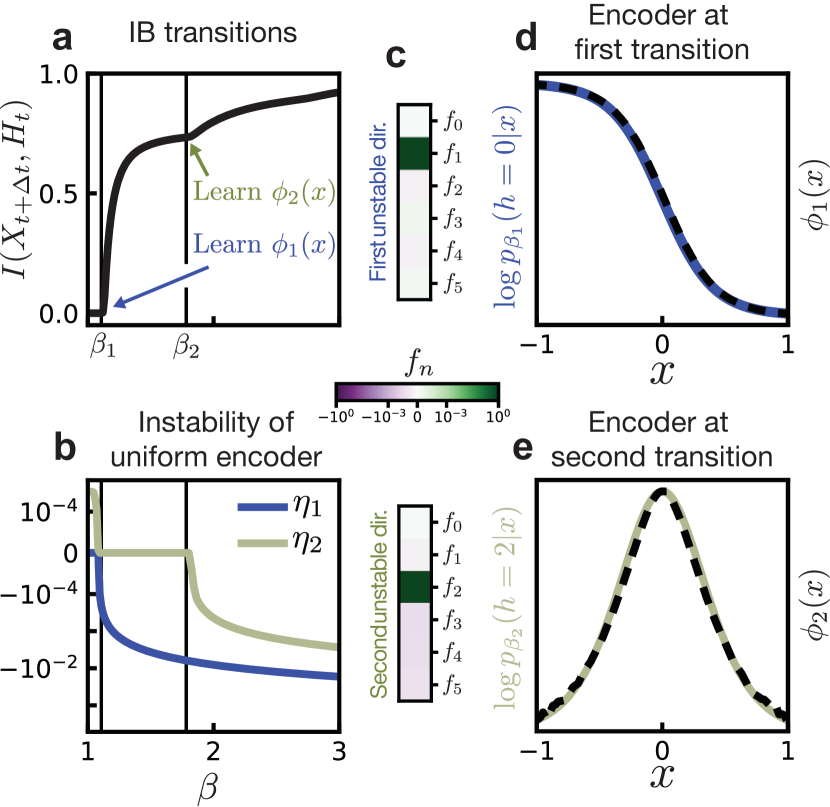
Figure 7: IB learns eigenfunctions of the adjoint transfer operator. (a) When the relative weight $\beta$ between both constraints in Eq. 1 is changed, more and more information can go through the encoder. This occurs in steps, where the spectral content of the transfer operator is included starting from eigenvalues with largest magnitude (i.e., the slowest ones). (b) Transitions are characterized by the appearance of negative eigenvalues in the spectrum of the Hessian of the IB loss function. Here we consider the Hessian evaluated at the uniform encoder $p(h|x)=N_{H}^{-1}$. The IB transitions $\beta_{1}\approx 1.1$ and $\beta_{2}\approx 1.8$ correspond to the appearence of negative eigenvalues of the Hessian. (c) The unstable directions are dominated by single components (note the color scale is logarithmic). (d) At the first transition, the logarithm of the encoder is given by the eigenfunction $\phi_{1}(x)$, up to rescaling ($y$-axis is shown in arbitrary units). (e) Likewise, at the second transition the encoder is given by $\phi_{2}(x)$.

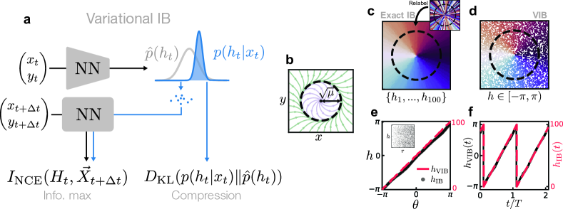
Figure 8: Variational IB extends exact IB. (a) Variational IB optimizes the variational objective directly from samples, in contrast to exact IB which requires an estimation of the full conditional distribution $p(x_{x+\Delta t}|x_{t})$. Values of $h_{t}$ are drawn from a “latent” distribution $p(h|x)$, from which one can estimate the mutual information $I(X_{t+\Delta t},H_{t})$. The compression term is approximated by the Kullback-Leibler divergence between the learned $p(h|x)$ and a variational ansatz for the marginal $\hat{p}(h)$. (b) Phase portrait for a dynamical system above a Hopf bifurcation. (c) Exact IB learns (up to permutations) an encoding $h$ which corresponds to the polar angle coordinate $\theta$. (d) Variational IB similarly learns the correct encoding, directly from samples. (e) Correspondence between IB encodings and the angle coordinate $\theta$. The encoding learned by VIB is independent of $r$ (inset). (f) Time dependence of the encoded variable $h_{t}$.

IB finds transfer operator eigenfunctions by optimizing an information theoretic-objective that makes no reference to physics or dynamics. This suggests it may be used for the discovery of slow variables in situations where one lacks physical intuition. The utility of exact IB for this purpose is limited because it requires knowledge of the exact conditional distribution $p(x_{t+\Delta t}|x_{t})$ which is difficult to estimate in many real-world scenarios. Fortunately however, the IB optimization problem can be replaced by an approximate variational objective introduced in Ref. [30] that can be solved with neural networks. In the remainder of this paper, we show how to implement these networks for the discovery of slow variables directly from data.

In place of the optimal encoder, we instead search for one which minimizes a tractable upper bound on the Lagrangian Eq. 1. To achieve this, the first (compression) term is upper-bounded as

$$I(X_{t};H_{t})\leq D_{\text{KL}}(p(h|x)\lVert\hat{p}(h))$$

where $\hat{p}(h)$ is a variational approximation to the marginal $p(h)$. The second term is lower-bounded by a noise-contrastive estimate of the mutual information [50],

$$I(X_{t+\Delta t};H_{t})\geq I_{\text{NCE}}(X_{t+\Delta t};H_{t}),$$

which can be computed directly from samples, and does not require access to the full distribution $p(h_{t},x_{t+\Delta t})$ (see Appendix F for details). The procedure for finding the optimal encoder in variational IB (VIB) are shown schematically in Fig. 8a; compare this to the procedure for exact IB shown in Fig. 5.

We now show that VIB learns an encoding consistent with exact IB, i.e. one which depends only on the dominant transfer operator eigenfunctions. We consider the example of a Hopf oscillator given by the dynamical system

$$\dot{r} =r(\mu-r^{2}),$$

$$\dot{\theta} =\omega.$$ (11)

Equation (11) is the normal form (in polar coordinates) for dynamics near a Hopf bifurcation [51]. For $\mu>0$ this system exhibits a circular limit cycle of radius $\sqrt{\mu}$ (Fig. 8b). In Appendix G we show that this system has infinite purely imaginary eigenvalues $\lambda_{n}=in\omega$ and that as a result, encoders which exactly encode the angle coordinate, $p(h|r,\theta)\propto\delta(h-\theta)$, are solutions of the IB optimization problem.

The exact IB calculation breaks down for perfectly deterministic dynamics, hence we add a small amount of white noise to the dynamics. While this slightly perturbs the spectral content of the transfer operator, we still find our results to be consistent with the those expected for the deterministic case (see Appendix G). As we increase the size of the encoding alphabet $N_{H}$, the encoder partitions space by finer and finer angular wedges. The learned encoding is invariant under permutations of the encoded symbols. Upon reordering, we find that, for large alphabets $N_{H}\gg 1$, the encoder indeed approximates $p(h|r,\theta)\propto\delta(h-\theta)$ as expected (Fig. 8c).

Using VIB, we learn a continuous $h_{t}$ which can be computed directly from samples of the state variable. The encoding $h_{t}$ learned by VIB closely approximates the angle coordinate (Fig. 8e-f) and is nearly uncorrelated with $r$ (inset). This shows that our mathematical results illustrated for exact IB in Sec. V hold also in the approximate framework of VIB. In Appendix F we verify this also for the Lorenz system, a standard example of chaotic dynamics.

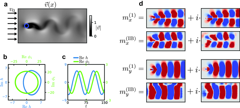
Figure 9: VIB for high-dimensional simulated fluid flow. (a) A fluid flows into the system with uniform velocity $v_{0}$ in the $x$-direction and passes a disk-shaped obstacle, which perturbs the fluid and causes vortex shedding behind the object in a so-called von Kármán street. (b) The dynamics in latent space (blue) are very regular, traversing a nearly circular trajectory. For comparison we show the evolution of the mode amplitudes obtained by projecting the velocity field onto the first DMD mode (green). (c) Time evolution of one component of the latent variable ($h_{1}$, blue) as well as the DMD mode amplitude (green). (d) Comparison of the first Koopman mode obtained from DMD ($\bm{m}^{(1)}$) and from VIB ($\bm{m}^{(\text{IB})}$). Koopman modes from VIB are computed as gradients of the latent encoding variables as described in the main text. Red corresponds to positive values and blue to negative; the magnitudes of the modes are not directly comparable.

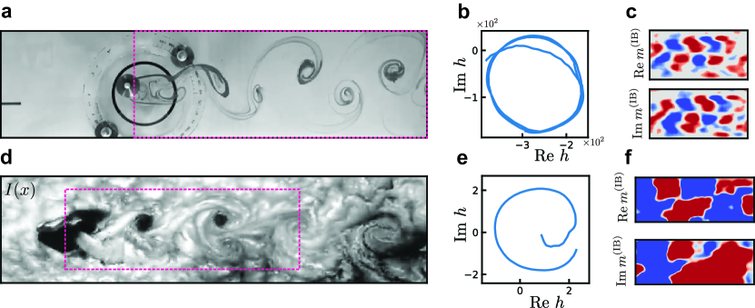
Figure 10: Two experimental case studies: slow dynamics in flow past a cylinder and atmospheric vortices. (a) Frame of experimentally-imaged von Kármán street extracted from Ref. [52]. Here we show the grayscale image fed as input into the VIB neural network. (b) Trajectory of learned encoding variables in the latent space. (c) Gradients of the latent encoding variables with respect to the input field. Note the similar symmetry as $\bm{m}^{(\text{IB})}_{x}$ in (d). (d) Satellite image of von Kármán street visible in clouds behind Guadalupe Island extracted from Ref. [53]. (e) The trajectory of learned encoding variables in the latent space is nearly circular, despite only having access to one full cycle during training. (f) Gradients of the latent encoding variables with respect to the input field. Again, note the glide symmetry in $\partial h_{0}/\partial I$. This structure is less clear in $\partial h_{1}/\partial I$.

One benefit of the variational formulation of IB is that it may be applied directly to large datasets. Here we provide numerical evidence showing that the results of the previous sections remain valid for high-dimensional systems by considering a simulated fluids dataset. We then turn to experimental data to show that even in the presence of large noise and small sample sizes, our framework allows for an interpretation of VIB latent variables as approximate transfer operator eigenfunctions.

We first consider simulations of two-dimensional fluid flow past a disk [54]. The system is characterized by a high-dimensional velocity field $\bm{v}(x)\in\mathbb{R}^{2\times N_{\text{pixels}}}$, where $N_{\text{pixels}}\sim\mathcal{O}(10^{5})$ (Fig. 9a). Fluid flows in from the left boundary with a constant velocity $v_{0}\hat{e}_{x}$ past a disk of unit diameter. At Reynolds number $\text{Re}\gtrsim 150$, the fluid undergoes periodic vortex shedding behind the disk, forming what is known as a von Kármán street.

This system is well approximated by linear dynamics, so that eigenfunctions of the adjoint transfer operator are given by linear functions of the state variable,

$$\phi_{n}[\bm{v}]=\langle\bm{v}(\bm{x}),\bm{m}^{(n)}(\bm{x})\rangle,$$ (12)

where $\bm{m}^{(n)}$ is the $n$-th “Koopman mode” and angled brackets denote integration over space. To compute these modes and the corresponding transfer operator spectrum, we use dynamic mode decomposition (DMD; see Appendix H) [55, 56]. The eigenfunctions for this system are in general complex, and come in conjugate pairs: $\phi_{2}(x)=\phi^{*}_{1}(x)$. In this situation any linear combination of $\phi_{1}$ and $\phi_{2}$ will decay at the same rate, and hence we expect VIB to learn some arbitrary combination of the two dominant eigenfunctions, or equivalently a combination of the real and imaginary parts of $\phi_{1}$. We therefore allow VIB to learn a two-dimensional encoding variable $[h_{0},h_{1}]$, so that it can learn the complete first eigenfunction rather than only the real or imaginary part. For the purposes of comparing our learned variable with $\phi_{1}$, we construct a complex $h=h_{0}+ih_{1}$ out of the two learned components and rotate the true eigenfunction by a complex constant $\phi_{1}\rightarrow e^{i\theta}\phi_{1}$ so that the real and imaginary parts of $\phi_{1}$ and $h$ coincide.

Our learned latent variables are oscillatory with the correct frequency as shown in Fig. 9b-c. The fact that the latent variables oscillate as expected does not on its own imply that they are learning the correct eigenfunctions: there may be many such functions which exhibit the same oscillatory behavior, for example the flow velocity at one well-chosen pixel.

To distinguish these cases, we must identify whether the learned functions $h_{i}[\bm{v}]$ are of the form Eq. (12). This can be done by examining gradients of the network with respect to the input field

$$\frac{\partial h}{\partial v_{j}}=m^{(\text{IB})}_{j}+g_{\text{res},j}(\bm{v}(\bm{x}))$$ (13)

where we have separated the part of the gradient which is independent of $\bm{v}$ from a residual part which is dependent on $\bm{v}$. Gradients of the true eigenfunctions are given simply by

$$\frac{\partial\phi_{n}}{\partial v_{j}}=m_{j}^{(n)}.$$ (14)

We can then directly compare our latent variables with the true eigenfunctions by comparing their derivatives. If $h$ corresponds to the true eigenfunction, we expect that $\bm{m}^{(\text{IB})}$ is approximately equal to the Koopman mode $\bm{m}^{(1)}$, and that $\bm{g}_{\text{res}}$ is small. We indeed find this to be the case; Fig. 9d shows these gradients averaged over several instantiations of the neural network, which corresponds strongly to the true mode. Details concerning both the averaging procedure and the residuals $\bm{g}_{\text{res}}$ can be found in Appendix H. This suggests that VIB not only recovers the essential oscillatory nature of the dynamics, but does so by learning the correct slowly varying functions of the state variable given by the Koopman eigenfunctions.

VII DVIB for model reduction directly from experimental movies

The scenario above is characterized by high-dimensional data and few samples; training was performed with only $\sim 400$ samples. We now demonstrate that our framework continues to hold approximately and yield interpretable latent spaces even for real-world fluid flow datasets scraped directly from videos on Youtube [52, 53].

The first shows a von Kármán street which forms as water passes by a cylindrical obstacle at Reynolds number 171, with flow visualized by a dye injected at the site of the obstacle [52]. We take a background-subtracted grayscale image of the flow field as our input (Fig. 10a) and task VIB with learning a two-dimensional latent variable as above. Also here, VIB learns oscillatory dynamics of the latent variables (Fig. 10b). We visualize the function learned by the encoder by considering gradients of the latent variables, which show the same structure as those obtained for the $x$ component of the simulated data (Fig. 10c). This is expected, as the $x$-component of the velocity field has similar glide reflection symmetry as the intensity image.

Finally, we apply VIB to a von Kármán street arising due to flow around Guadalupe Island, which was imaged by a National Oceanic and Atmospheric Administration (NOAA) satellite [53] (Fig. 10d). The video consists of only 62 frames, and the von Kármán street undergoes a single oscillation. Even with this small amount of data, our VIB method learns latent variables which capture this oscillation and have the expected dependence on the input variables (Fig. 10e-f). As in the first experimental example, the gradients of the encoding variables show the glide symmetry of $m_{x}$ due to the symmetry of the intensity pattern in Fig. 9d. This symmetry is less clear in the component $\frac{\partial h_{1}}{\partial I(x)}$, which is likely due to the fact that the von Kármán street is not as fully formed in this data as in our previous examples: the vortices in the lower half of the street are less apparent than those in the top half.

VIII Conclusion

We have related information-theoretical properties of dynamical systems to the spectrum of the transfer operator. We illustrate our findings on several simple and analytically tractable systems, and turn them into a practical tool using variational IB, which learns an encoding variable with a neural network. The latent variables of these networks can be interpreted as transfer operator eigenfunctions even though the network was not explicitly constructed to learn these: it optimizes a purely information-theoretic objective that contains no knowledge of a transfer operator or dynamics. This allows one to harness the power of neural networks to learn physically-relevant latent variables. Our results may be particularly useful for discovering slow variables in complex systems where one lacks physical intuition.

IX Acknowledgements

M.K.-J. would like to thank Zohar Ringel for discussions. M.S.S. acknowledges support from a MRSEC-funded Graduate Research Fellowship (DMR-2011854). M.K.-J. gratefully acknowledges financial support from the European Union’s Horizon 2020 programme under Marie Sklodowska-Curie Grant Agreement No. 896004 (COMPLEX ML). D.S.S. acknowledges support from a MRSEC-funded Kadanoff–Rice fellowship and the University of Chicago Materials Research Science and Engineering Center (DMR-2011854). V.V. acknowledges support from the Simons Foundation, the Complex Dynamics and Systems Program of the Army Research Office under grant W911NF19-1-0268, the National Science Foundation under grant DMR-2118415 and the University of Chicago Materials Research Science and Engineering Center, which is funded by the National Science Foundation under award no. DMR-2011854.

Appendix A Information bottleneck

The information bottleneck was originally formulated in Ref. [26] as a rate distortion problem. Rate distortion theory describes how to maximally compress a signal (i.e. minimize its communication rate) such that it remains minimally distorted, which, however, presupposes the knowledge of a distortion function specifying which features need to be preserved[28]. In Ref. [26], Tishby et al. introduce a variant of the problem where the a priori unknown distortion function is not used, but rather one seeks to ensure that the compression retains information about an auxiliary variable $Y$ correlated with the signal. As the correlations with $Y$ define implicitly the relevant features of the signal to be preserved, $Y$ is called the relevance variable. Concretely, we call $X$ the source signal, and $H$ denotes the compressed signal. The random variables form a Markov chain $H\leftrightarrow X\leftrightarrow Y$, meaning that $H$ and $Y$ are conditionally independent given $X$:

$$p(y|h,x) =p(y|x)p(h,x)$$

$$p(h|x,y) =p(h|x)p(y,x)$$

As noted in the main text, the IB optimization objective is given by the Lagrangian

$$\mathcal{L}_{\text{IB}}[p(h|x)] =I(X,H)-\beta I(Y,H).$$ (15)

To enforce normalization of the $p(h|x)$ one introduces a Lagrange multiplier $\lambda(x)$ so that the full optimization function is

$$\begin{split}\mathcal{L}_{\text{IB}}[p(h|x)]&=\sum_{x,h}p(h|x)p(x)\log\frac{p(h|x)}{p(h)}\\ &\qquad-\beta\sum_{y,h}p(y,h)\log\frac{p(y,h)}{p(h)p(y)}\\ &\qquad+\sum_{x}\lambda(x)\left(1-\sum_{h}p(h|x)\right).\end{split}$$ (16)

The encoder which optimizes this objective can be solved for exactly. Using the following functional derivatives,

$$\frac{\delta}{\delta p(h|x)}p(h^{\prime}) =\delta(h-h^{\prime})p(x)$$

$$\frac{\delta}{\delta p(h|x)}p(h^{\prime},y^{\prime}) =\delta(h-h^{\prime})p(x,y^{\prime}),$$

one can compute the derivative of the Lagrangian. By evaluating the derivative and setting to zero, one finds

$$\log p(h|x)=\log p(h)-\beta\sum_{y}p(y|x)\log\frac{1}{p(y|h)}-\lambda(x)$$

which can be rearranged to give the optimal encoder

$$p(h|x)=\frac{p(h)}{N(x)}\exp\left[-\beta D_{KL}(p(y|x)\|p(y|h))\right].$$ (17)

By absorbing terms which only depend on $h$ and $x$ into $p(h)$ and $N(x)$, respectively, the encoder can be expressed as

$$p(h|x)=\frac{p(h)}{N(x)}\exp\left[\beta\int dy\,p(y|x)\log p(y|h)\right].$$ (18)

When $\beta<1$, it follows from the data processing inequality $I(X,H)\geq I(Y,H)$ that Eq. (15) is minimized by a trivial encoder $p(h|x)=p(h)$. In this case, $\mathcal{L}_{\text{IB}}=0$ and no information passes through the bottleneck. As $\beta$ is increased, more information is allowed through the bottleneck until the relevant variables begin to gain a dependence on the state $x$. This occurs suddenly for a certain value of $\beta=\beta_{1}>1$ at which the encoder becomes non-uniform and $I(H,X)$ becomes non-zero. This is referred to as an IB transition; for increasing $\beta$, there may be a sequence of transitions at $\beta_{2},\beta_{3},...$ etc.

Appendix B Transfer operators

In this work we consider dynamical systems given by a Langevin equation

$$\dot{\bm{x}}=\bm{f}(\bm{x})+\sqrt{2D(\bm{x})}\bm{\xi}(t)$$ (19)

where the first term is the deterministic part of the dynamics, and the second term corresponds to noise, where

$$\langle\xi_{i}(t)\xi_{j}(t^{\prime})\rangle=C_{ij}\delta(t-t^{\prime}).$$

This framework captures purely deterministic dynamics, which are obtained by setting $D=0$.

The transfer operator describes the evolution of probability distributions. For dynamics given by a Langevin equation, probability distributions evolve according to the corresponding Fokker-Planck equation

$$[\mathcal{L}\rho](\bm{x})=\partial_{t}\rho(\bm{x})=-\partial_{i}(f_{i}(\bm{x})\rho(\bm{x}))+\partial_{i}\partial_{j}(D(\bm{x})C_{ij}\rho(\bm{x})).$$

Here we recognize $\mathcal{L}$ as the infinitesimal generator of the transfer operator $U$: evolution for a time $t$ is given by $U=\text{e}^{t\mathcal{L}}$.

The adjoint operator is given by the so-called backward Kolmogorov equation, and it describes the evolution of functions $\phi$.

$$\mathcal{L}^{\dagger}\phi(x)=f_{i}(\bm{x})\partial_{i}(\phi(\bm{x}))+D(\bm{x})C_{ij}\partial_{i}\partial_{j}(\phi(\bm{x})).$$ (20)

For $D=0$, $\mathcal{L}$ is the generator of the Perron-Frobenius operator, while its adjoint is the Koopman operator [19].

Appendix C Derivation

Here we derive the form of the optimal encoder given in Eq. 7 and the approximation at the first transition. In Ref. [26], it is shown that the encoding minimizing Eq. 1 satisfies the implicit equation

$$\!\!\!\!p_{\beta}^{*}(h|x)=\frac{p_{\beta}^{*}(h)}{\mathcal{N}(x)}\,\exp\left(-\beta D_{\text{KL}}\left[p_{X_{t+\Delta t}|X_{t}}\big{|}\big{|}p_{X_{t+\Delta t}|H_{t}}\right]\right)$$ (21)

where $\mathcal{N}$ is a normalization factor ensuring $\int\text{d}h\,p_{\beta}^{*}(h|x)=1$, and

$$p_{\beta}^{*}(h)\equiv p^{*}_{H_{t};\beta}(h)=\int\text{d}x\,p_{H_{t}|X_{t};\beta}^{*}(h|x)p_{X_{t}}(x).$$ (22)

The Kullback-Leibler divergence between two probability distributions $p(x)$ and $q(x)$ is defined by

$$D_{\text{KL}}[p||q]=\int\text{d}x\,p(x)\,\log\frac{p(x)}{q(x)};$$ (23)

in the $D_{\text{KL}}$ in (21), the integration is done with respect to the common random variable $X_{t+\Delta t}$ of the two conditional distributions.

Equation (21) contains the conditional distribution $p_{X_{t+\Delta t}|H_{t}}$, which is the composition of two operations: decoding (going from $H_{t}$ to $X_{t}$) and time evolution (going from $X_{t}$ to $X_{t+\Delta t}$). The decoding is performed using Bayes’ theorem $p_{X_{t}|H_{t}}p_{H_{t}}=p_{H_{t}|X_{t}}p_{X_{t}}$, so that we have

$$p_{X_{t+\Delta t}|H_{t}}=\int_{X_{t}}p_{X_{t+\Delta t}|X_{t}}\,p_{H_{t}|X_{t}}\,\frac{p_{X_{t}}}{p_{H_{t}}}.$$ (24)

Note the appearance of the encoder $p_{H_{t}|X_{t}}$, making Eq. (21) only an implicit solution of the optimization problem.

To arrive at the expression for the encoder Eq. (7), we write the conditional distribution in terms of right and left eigenvectors of $U$. As mentioned in Sec. II, we neglect $U_{\text{ess}}$, which is the operator corresponding to the essential spectrum. The essential spectrum is the part of the spectrum that is not the discrete spectrum; by neglecting it, we are assuming that the essential radius $\rho_{\text{ess}}$ (the maximum absolute value of eigenvalues in the essential spectrum) is small enough compared to the first few eigenvalues $|\lambda_{n}|$ in the point spectrum. While purely deterministic systems may exhibit a large essential radius, the introduction of noise causes the essential spectrum to shrink or disappear [33, 34]. We can then write the conditional distribution in terms of right and left eigenvectors of $U$,

$$p_{X_{t+\Delta t}|X_{t}}(x|x^{\prime}) =\sum_{n}\text{e}^{\lambda_{n}\Delta t}\rho_{n}(x)\phi_{n}(x^{\prime}).$$ (25)

The Kullback-Leibler divergence in Eq. (7) can be represented as a sum of two terms,

$$D_{\text{KL}}[...] =\int\text{d}x_{t+\Delta t}\,p(x_{t+\Delta t}|x_{t})\,\log p(x_{t+\Delta t}|x_{t})$$

$$\quad-\int\text{d}x_{t+\Delta t}\,p(x_{t+\Delta t}|x_{t})\,\log p(x_{t+\Delta t}|h_{t}).$$ (26)

The first term has no dependence on $h$ and can hence be absorbed into the normalization $\mathcal{N}(x)$. Plugging the decomposition Eq. (25) into the second term leads directly to

$$p_{\beta}^{*}(h|x)=\frac{1}{\mathcal{N}(x)}\,p_{\beta}^{*}(h)\,\exp\left[\beta\sum_{n}\text{e}^{\lambda_{n}\Delta t}\phi_{n}(x)f_{n}(h)\right]$$ (27)

where

$$f_{n}(h)=\int\text{d}x_{t+\Delta t}\,\rho_{n}(x_{t+\Delta t})\log p(x_{t+\Delta t}|h),$$ (28)

which can be understood as a quasi-cross entropy between the right eigenvector $\rho_{n}$ and the distribution on $x_{t+\Delta t}$ obtained by decoding $h$. Equation (27) depends only on the existence of the spectral decomposition; we have made no other assumptions on the dynamics (beyond Markovianity) up until this point.

Stability of the uniform encoder

In this section we derive our main result for the optimal encoder in the limit of high compression (small $\beta$).

Mathematical result – Consider a transfer operator $U$ with infinitesimal generator $\mathcal{L}_{U}$. Assume that $\mathcal{L}_{U}$ has a discrete spectrum with eigenvalues satisfying $0=\text{Re }\lambda_{0}>\text{Re }\lambda_{1}>\text{Re }\lambda_{2}\gg\text{Re }\lambda_{3}...$. Then, for $\beta$ just above the first IB transition $\beta_{1}$ so that $f_{n}(h)\rightarrow 0$, the optimal encoder is given approximately by

$$p^{*}_{\beta}(h|x)=\frac{1}{\mathcal{N}(x)}p^{*}_{\beta}(h)\,\exp\left(\beta\,\text{e}^{\lambda_{1}\Delta t}\phi_{1}(x)f_{1}(h)\right)$$ (29)

with corrections due to the second eigenfunction given by $f_{2}(h)\approx f_{1}(h)\text{e}^{-\Gamma\Delta t}+\mathcal{O}(\text{e}^{-2\Gamma\Delta t})$ where $\Gamma=\lambda_{1}-\lambda_{2}>0$ denotes the spectral gap.

To show this we compute the $f_{n}(h)$ coefficients at the onset of instability. The instability at the first IB transition at $\beta=\beta_{1}$ corresponds to the emergence of negative eigenvalues in the Hessian of the IB loss,

$$\frac{\partial^{2}}{\partial f_{n}(h_{i})\partial f_{m}(h_{j})}\mathcal{L}_{\text{IB}}.$$ (30)

Similar stability approaches have been studied in other contexts within IB in [35, 57, 38].

For concreteness, we consider a discrete state $x\in\{1,...,N_{X}\}$ and discrete encoding $h\in\{1,...,N_{H}\}$. We express the encoder as in Eq. 7

$$p_{\beta}^{*}(h_{\mu}|x_{i})=\frac{f_{0}(h_{\mu})\exp\left[\beta\sum_{n}\text{e}^{\lambda_{n}\Delta t}\phi_{n}(x_{i})f_{n}(h_{\mu})\right]}{\sum_{h_{\lambda}}f_{0}(h_{\lambda})\exp\left[\beta\sum_{n}\text{e}^{\lambda_{n}\Delta t}\phi_{n}(x_{i})f_{n}(h_{\lambda})\right]}$$ (31)

In the following, we simplify notation as

$$p(h_{\mu}|x_{i})=\frac{f_{0}^{\mu}\exp\left[\sum_{n}\tilde{\phi}_{n}(x_{i})f_{n}^{\mu}\right]}{\sum_{h_{\lambda}}f_{0}^{\lambda}\exp\left[\sum_{n}\tilde{\phi}_{n}(x_{i})f_{n}^{\lambda}\right]}$$ (32)

where $\tilde{\phi}_{n}(x_{i})=\beta\text{e}^{\lambda_{n}\Delta t}\phi_{n}(x_{i})$. For the uniform encoder, $f_{n}^{\mu}=0$ for all $n\neq 0$. To compute the Hessian at the uniform encoder, we use that, for $n\neq 0$,

$$\partial_{n}^{\mu}p(h_{\nu}|x_{i}) \equiv\frac{\partial}{\partial f_{n}^{\mu}}p(h_{\nu}|x_{i})$$ (33)

$$=p(h_{\nu}|x_{i})\tilde{\phi}_{n}(x_{i})\left(\delta_{\mu\nu}-p(h_{\mu}|x_{i})\right)$$ (34)

and for $n=0$,

$$\partial_{0}^{\mu}p(h_{\nu}|x_{i}) =p(h_{\nu}|x_{i})\frac{1}{f_{0}^{\mu}}\left(\delta_{\mu\nu}-p(h_{\mu}|x_{i})\right).$$ (35)

Hereafter we assign $\tilde{\phi}_{0}=\frac{1}{f_{0}^{\mu}}$, taking care to track the correct Greek index which otherwise is not present for $\tilde{\phi}_{n}$ (in the following, $n$ is always paired with $\mu$ and $m$ always with $\nu$). Following from the above relations, we find

$$\partial_{n}^{\mu}p(h_{\nu}) =\sum_{x_{i}}p(x_{i})p(h_{\nu}|x_{i})\tilde{\phi}_{n}(x_{i})\left(\delta_{\mu\nu}-p(h_{\mu}|x_{i})\right).$$ (36)

We are now in a position to calculate the Hessian of the Lagrangian; we omit the messy algebra and state the result. The key steps in the derivation is the fact that $\sum_{\lambda}\partial^{\mu}_{n}p(h_{\lambda})=0$ (by exchanging sum and derivative), and that $p(h_{\mu}|x_{i})|_{\bm{f}=0}=p(h_{\mu})$. The compression term is given by

$$\partial_{n}^{\mu}\partial_{m}^{\nu}I(X,H) =\left(\langle\tilde{\phi}_{n}\tilde{\phi}_{m}\rangle-\langle\tilde{\phi}_{n}\rangle\langle\tilde{\phi}_{m}\rangle\right)$$

$$\qquad\times\left(\delta_{\mu\nu}p(h_{\mu})-p(h_{\nu})p(h_{\mu})\right)$$

and the information maximization term is

$$\partial_{n}^{\mu}\partial_{m}^{\nu}I(Y,H) =\left(\left\langle\frac{\langle\tilde{\phi}_{n}\rangle_{p(\cdot,y)}\langle\tilde{\phi}_{m}\rangle_{p(\cdot,y)}}{p(y)^{2}}\right\rangle-\langle\tilde{\phi}_{n}\rangle\langle\tilde{\phi}_{m}\rangle\right)$$

$$\qquad\times\left(\delta_{\mu\nu}p(h_{\mu})-p(h_{\nu})p(h_{\mu})\right)$$

Angled brackets with no subscript correspond to an average with respect to the steady state distribution, $\langle\cdot\rangle=\sum_{x_{i}}\cdot\,p(x_{i})$. For the second term, we retain the argument which is integrated over ($y$) for clarity. In sum, the Hessian of the Lagrangian is given by

$$H_{(\mu,n),(\nu,m)} =\left(\langle\tilde{\phi}_{n}\tilde{\phi}_{m}\rangle-\beta\left\langle\frac{\langle\tilde{\phi}_{n}\rangle_{p(\cdot,y)}\langle\tilde{\phi}_{m}\rangle_{p(\cdot,y)}}{p(y)^{2}}\right\rangle-(1-\beta)\langle\tilde{\phi}_{n}\rangle\langle\tilde{\phi}_{m}\rangle\right)\left(\delta_{\mu\nu}p(h_{\mu})-p(h_{\nu})p(h_{\mu})\right)$$ (37)

which lives in $\mathbb{R}^{(N_{X}\times N_{H})\times(N_{X}\times N_{H})}$; we index $H$ with a multi-index $(\mu,n)$. From the form of Eq. 37, we see that $H$ is given by a Kronecker (tensor) product

$$H_{(\mu,n),(\nu,m)} =A^{\beta}_{nm}\otimes G_{\mu\nu}.$$

Eigenvalues of $H$ are given by products of eigenvalues of $A^{\beta}$ and $G$, while eigenvectors are given by the tensor product of eigenvectors of $A^{\beta}$ and $G$. The appearance of unstable directions of the Hessian corresponds to the appearance of negative eigenvalues in its spectrum. As $G$ does not depend on $\beta$, zero-crossings of eigenvalues of $H$ therefore correspond to zero-crossings of eigenvalues in the spectrum of $A^{\beta}$.

We now show that the first component $f_{1}$ is selected at the first IB transition. From our assumption on the spectrum of $\mathcal{L}_{U}$, namely $0>\text{Re}\lambda_{1}>\text{Re}\lambda_{2}\gg\text{Re}\lambda_{3}...$ it follows that near the first IB transition the IB loss is given by

$$\mathcal{L}_{\text{IB}} =\begin{pmatrix}f_{1}\\ f_{2}\end{pmatrix}^{T}\begin{pmatrix}a_{11}&a_{12}\\ a_{12}&a_{22}\end{pmatrix}\begin{pmatrix}f_{1}\\ f_{2}\end{pmatrix}+\mathcal{O}(f_{n}^{3},\,\text{e}^{\lambda_{3}\Delta t})$$

with

$$a_{11} =\text{e}^{2\lambda_{1}\Delta t}\left(\langle\phi_{1}^{2}\rangle-\beta B_{11}\right)=\text{e}^{2\lambda_{1}\Delta t}\hat{a}_{11}$$

$$a_{12} =\text{e}^{(\lambda_{1}+\lambda_{2})\Delta t}\left(\langle\phi_{1}\phi_{2}\rangle-\beta B_{12}\right)=\text{e}^{(\lambda_{1}+\lambda_{2})\Delta t}\hat{a}_{12}$$

$$a_{22} =\text{e}^{2\lambda_{2}\Delta t}\left(\langle\phi_{2}^{2}\rangle-\beta B_{22}\right)=\text{e}^{2\lambda_{2}\Delta t}\hat{a}_{22},$$

where we have introduced the shorthand $B_{ij}=\left\langle\frac{\langle\tilde{\phi}_{i}\rangle_{p(\cdot,y)}\langle\tilde{\phi}_{j}\rangle_{p(\cdot,y)}}{p(y)^{2}}\right\rangle$. The stability of the uniform encoder at $f_{n}=0$ is given by the stability of the 2$\times$2 matrix above. The eigenvalues $\omega_{i}$ and eigenvectors $\bm{v}_{i}$ of this matrix can be computed explicitly,

$$\eta_{\pm} =\frac{1}{2}\left(\text{e}^{2\lambda_{1}\Delta t}\hat{a}_{11}+\text{e}^{2\lambda_{2}\Delta t}\hat{a}_{22}\pm D\right)$$

$$\bm{v}_{\pm} =\begin{pmatrix}\frac{-1}{2\text{e}^{(\lambda_{1}+\lambda_{2})\Delta t}\hat{a}_{12}}\left(-\text{e}^{2\lambda_{1}\Delta t}\hat{a}_{11}+\text{e}^{2\lambda_{2}\Delta t}\hat{a}_{22}\mp D\right)\\ 1\end{pmatrix}$$

where

$$D =(\text{e}^{4\lambda_{1}\Delta t}\hat{a}_{11}^{2}+2\text{e}^{2(\lambda_{1}+\lambda_{2})\Delta t}(2\hat{a}_{12}^{2}-\hat{a}_{11}\hat{a}_{22})$$

$$\qquad+\text{e}^{4\lambda_{2}\Delta t}\hat{a}_{22}^{2})^{1/2}.$$

In what follows, we will express quantities in terms of the spectral gap $\Gamma=\lambda_{1}-\lambda_{2}>0$. For example, the expression above can be written

$$D =\text{e}^{2\lambda_{1}\Delta t}\left(\hat{a}_{11}+\mathcal{O}(\text{e}^{-2\Gamma\Delta t})\right).$$

The first eigenvalue to become negative is $\eta_{+}$. We are interested in the ratio of the corresponding eigenvector components, $f_{1}/f_{2}=\bm{v}_{+,1}/\bm{v}_{+,2}$, which tells us how much the encoder will depend on the first eigenfunction $\phi_{1}(x)$ compared to the second. This ratio is given by

$$\frac{f_{1}}{f_{2}} =\frac{-\text{e}^{(\lambda_{1}-\lambda_{2})\Delta t}}{2\hat{a}_{12}}\left(-\hat{a}_{11}+\text{e}^{2(\lambda_{2}-\lambda_{1})\Delta t}\hat{a}_{22}-D\right)$$ (38)

$$=\frac{\text{e}^{\Gamma\Delta t}}{2\hat{a}_{12}}\left(2\hat{a}_{11}+\mathcal{O}(\text{e}^{-2\Gamma\Delta t})\right)$$ (39)

$$=\text{e}^{\Gamma\Delta t}\frac{\hat{a}_{11}}{\hat{a}_{12}}+\mathcal{O}(\text{e}^{-2\Gamma\Delta t}).$$ (40)

This suggests that we must make one additional assumption, which is that the factor $\hat{a}_{11}/\hat{a}_{12}$ is not small. This is true in the simple 2-, 3-, and 4-well systems considered in this work, where we observe $\hat{a}_{12}$ is typically small (hence the inverse is large).

Note that in this calculation, $\phi_{0}(x)$ is constant (following from the assumption of a non-degenerate eigenvalue at 0) so that the $f_{0}(h)$ factors can be absorbed into $p(h)$. This changes in the case of a degenerate ground state, which corresponds a situation where there are decoupled sectors in which the dynamics evolve independently. Then, each eigenfunction corresponding to the zero eigenvalue is piecewise constant on one of the independent sectors. The optimal encoder Eq. 29 will depend instead on $\phi_{0}(x)$, which identifies the independent sectors.

Appendix D Exact IB and Ulam approximations of the transfer operator

The optimal IB encoder can be found using the Blahut-Arimoto (BA) algorithm [28]. As described in detail in Refs. [26, 58], the algorithm is an iterative procedure, where the encoder at iteration $k+1$ is updated according to

$$\begin{cases}p_{k+1}(h|x_{t})=\frac{p_{k}(h)}{N_{k+1}(x)}\exp(-\beta D_{\text{KL}}(p(x_{t_{\Delta}t}|x_{t})\lVert p_{k}(x_{t+\Delta t}|h)))\\ p_{k+1}(h)=\sum_{x_{t}}p(x_{t})p_{k+1}(h|x_{t})\\ p_{k+1}(x_{t+\Delta t}|h)=\sum_{x_{t}}p(x_{t+\Delta t}|x_{t})p_{k+1}(x_{t}|h).\end{cases}$$

The first line simply plugs the previous estimate of the encoder in to Eq. 21 (and normalizes the distribution), while the following two lines update marginal and conditional distributions using the new estimate of the encoder. In Refs. [26, 58] it is shown that this algorithm converges.

The BA algorithm requires access to the conditional distribution $p(x_{t+\Delta t}|x_{t})$ for each $x_{t}$, as well as the steady state $p(x_{t})$. To solve the IB optimization problem we therefore need a numerical approximation of the transfer operator, which we obtain by an Ulam approximation [42, 43]. In brief, one divides space into bins and computes a finite-dimensional approximation to the conditional distribution as

$$P_{ij}=P(X_{t+\Delta t}=x_{j}|X_{t}=x_{i})=N_{i\rightarrow j}/N_{i},$$ (41)

where $N_{i}$ is the number of trajectories starting in bin $i$ and $N_{i\rightarrow j}$ the number of observed transitions from bin $i$ to bin $j$. The transfer operator is then approximately given by

$$Up(x_{j})\approx\sum_{x_{i}}P_{ij}p(x_{i}),$$ (42)

and eigenvalues and eigenvectors of $U$ can be computed by diagonalizing $P$.

Appendix E Rate of information decay

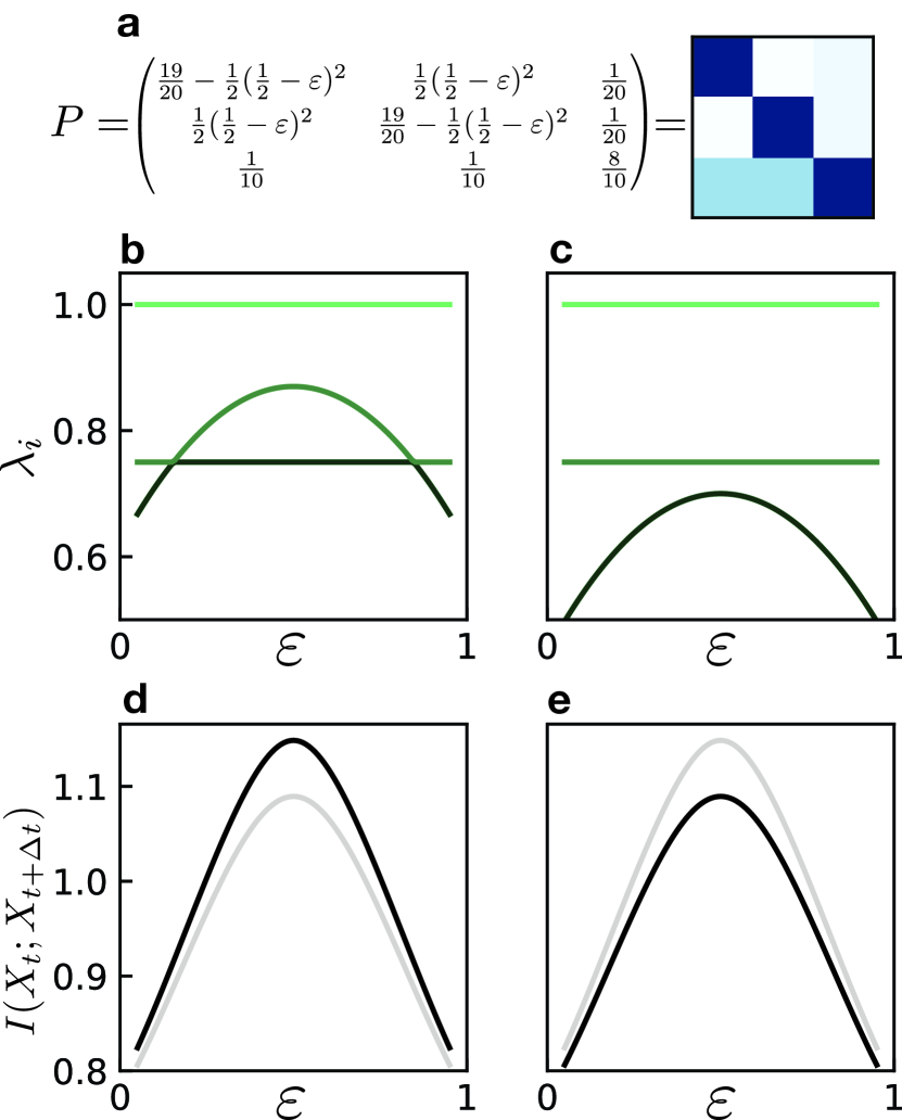
Figure S2: Information gain due to an eigenvalue pile-up. (a) To study the role of a gap closing compared to the pile-up of eigenvalues (beyond the dominant one) in the mutual information $I(X_{t};X_{t+\Delta t})$ we build a matrix $P$ with which we can tune the eigenvalues via a parameter $\varepsilon$. (b) Eigenvalues for the matrix shown in (a) with varying parameter values $\varepsilon$; for $\varepsilon\rightarrow 0.5$, the spectral gap $\lambda_{0}-\lambda_{1}$ closes. (c) Eigenvalues for the matrix shown in (a), but with all $\frac{1}{2}(\frac{1}{2}-\varepsilon)^{2}$ terms subtracted with a constant (here $1/8$). Here, the spectral gap $\lambda_{0}-\lambda_{1}$ does not close but there is an accumulation of eigenvalues at $\varepsilon\rightarrow 0.5$. (d-e) Mutual information for $\Delta t=1$ for the matrices in (b-c), respectively, as a function of $\varepsilon$. The curve from the other scenario is shown in gray for comparison. Both exhibit a clear peak in information which differs only slightly in magnitude, showing that the information peak in Fig. 3d-f of the main text is not due to the closing gap alone, but rather due to contributions from subdominant eigenvalues.

We consider the mutual information

$$I(X_{t},X_{t+\Delta t})=\sum_{x,y}p(y|x)p(x)\log\frac{p(y|x)}{p(y)}$$ (43)

where $x$ denotes values of the random variable $X_{t}$ and $y$ the values of $X_{t+\Delta t}$. We further consider dynamics which can be given by a transfer operator $U$ with integral kernel $p(y|x)$ that can be spectrally decomposed as

$$p(y|x)=\sum_{n}e^{\lambda_{n}t}\rho_{n}(y)\phi_{n}(x),$$ (44)

where $\lambda_{0}=0$, $\phi_{0}=\text{const}$ and $\rho_{0}(y)$ is the steady state distribution. The mutual information can then be written

$$I(X_{t},X_{t+\Delta t}) =\sum_{x,y}\sum_{n}e^{\lambda_{n}\Delta t}\rho_{n}(y)\phi_{n}(x)p(x)\log\left(1+\sum_{m>0}e^{\lambda_{m}\Delta t}\frac{\rho_{m}(y)}{p(y)}\phi_{m}(x)\right)$$ (45)

$$=\sum_{n,m>0}e^{(\lambda_{n}+\lambda_{m})\Delta t}\sum_{x,y}\phi_{n}(x)\phi_{m}(x)p(x)\frac{\rho_{n}(y)\rho_{m}(y)}{p(y)}$$ (46)

$$\quad+\sum_{n,m,\ell>0}e^{(\lambda_{n}+\lambda_{m}+\lambda_{\ell})\Delta t}\sum_{x,y}\phi_{n}(x)\phi_{m}(x)\phi_{\ell}(x)p(x)\frac{\rho_{n}(y)\rho_{m}(y)\rho_{\ell}(y)}{p(y)}+...$$ (47)

For long times, the contribution of $\lambda_{1}$ dominates, with the remaining terms decaying as $\text{e}^{(\lambda_{n}-\lambda_{1})\Delta t}$ for $n\geq 2$. Retaining only the first term, we see

$$I(X_{t},X_{t+\Delta t}) =e^{2\lambda_{1}\Delta t}\sum_{x}\phi^{2}_{1}(x)p(x)\sum_{y}\frac{\rho_{1}(y)^{2}}{p(y)}.$$ (48)

For short times, other eigenvalues will also contribute to the mutual information (Fig. S2).

Appendix F Variational IB

Exactly solving the IB problem in principle requires access to the full distribution $p(y,x)$, where $x$ is the variable to be compressed and $y$ is the relevance variable. One way around this is via so-called Deep Variational IB as introduced in Ref. [30]. The key result from [30] is an upper bound on the IB objective

$$\mathcal{L}_{\text{IB}}=I(X;H)-\beta I(Y;H).$$ (49)

To compute the first term, [30] introduces a variational ansatz for the marginal $\hat{p}(h)$. It follows from positivity of the Kullback-Leibler divergence $D_{\text{KL}}(p(h)\lVert\hat{p}(h))$ that

$$\int dhp(h)\log p(h)\geq\int dhp(h)\log\hat{p},$$ (50)

and hence

$$I(X,H) \leq\int dxdhp(h|x)p(x)\log\frac{p(h|x)}{\hat{p}(h)}$$ (51)

$$=\mathbb{E}_{x}D_{\text{KL}}(p(h|x)\lVert\hat{p}(h)).$$ (52)

If $p(h|x)$ and $\hat{p}(h)$ are chosen properly, the Kullback-Leibler can be expressed analytically which enables gradients to be effectively computed. As in Ref. [30], we take a Gaussian ansatz for $p(h|x)$ and let the marginal $\hat{p}(h)$ be a spherical unit-variance Gaussian. More concretely, encoded variables $H_{t}$ are sampled from $p(H_{t}|X_{t})$ by computing

$$h_{t}=f_{W}(x_{t})+\sigma_{W}(x_{t})\eta,$$ (53)

where $f_{W}$ and $\sigma_{W}$ are deterministic functions modeled by neural networks with parameters (weights) $W$, and $\eta$ is a Gaussian random variable with unit variance.

To bound the entire loss from above, we must bound $I(Y,H)$ from below. We do this using the noise-contrastive estimate of the mutual information introduced in Ref. [50]. This recasts the problem as one of distinguishing samples from the distributions $p(y|h)$ and $p(y)$. Given a batch of $B$ pairs $(y,h)$ and one particular value $h_{i}$, one asks what the probability is that a sample $y_{j}$ is from $p(y|h_{i})$ (is a positive sample) and not $p(y)$ (is a negative sample). This probability is

$$p(y_{j}=\text{pos}|h_{i})=\frac{\frac{p(y_{i}|h_{i})}{p(y_{i})}}{\sum_{k}^{B}\frac{p(y_{k}|h_{i})}{p(y_{k})}},$$ (54)

where $i$ is the index of the positive sample. The log likelihood of these probabilities,

$$\mathbb{E}[-\log p(y_{j}=\text{pos}|h_{i})],$$ (55)

where the expectation is taken over indices $i$ and $j$, is closely related to the mutual information $I(Y,H)$. In the limit of infinite samples $B\rightarrow\infty$, this quantity is given by

$$-\int dydh\,p(h)p(y|h)\log p(y_{j}=\text{pos}|h_{i})=\log B-I(Y,H).$$ (56)

If one had access to the probabilities $p(y_{i}=\text{pos}|h)$ appearing in Eq. 55, the mutual information could thus be easily determined. One attempts to estimate these probabilities by introducing a variational ansatz $f(y,h)$ to approximate the density ratio $\frac{p(y|h)}{p(y)}$. Typically this $f$ is represented by a neural network. One can then obtain a bound on the mutual information by minimizing

$$\mathcal{L}_{B}=\mathbb{E}\left[-\log\frac{f(y_{i}|h_{i})}{\sum_{k}^{B}f(y_{k}|h_{i})}\right],$$ (57)

from which the InfoNCE estimate of the mutual information can be calculated as

$$I_{\text{NCE}}(Y,H)=\log B-\mathcal{L}_{B}\leq I_{\text{true}}(Y,H).$$ (58)

The full objective to be minimized is given by

$$\mathcal{L}_{\text{VIB}}=D_{KL}(p(H_{t}|X_{t})\lVert\hat{p}(H_{t}))-\beta I_{\text{NCE}}(X_{t+\Delta t};H_{t}).$$ (59)

This loss is evaluated on batches of sample pairs $\{(x^{(1)}_{t},x^{(1)}_{t+\Delta t}),(x^{(2)}_{t},x^{(2)}_{t+\Delta t}),...\}$. A minimum is found via stochastic gradient descent.

The VIB loss Eq. 59 is very similar to the loss function for a time-lagged $\beta$-variational autoencoder ($\beta$-VAE) [59], which have a form $\mathcal{L}=D_{KL}-\mathcal{L}_{\text{rec}}$, where the reconstruction term $\mathcal{L}_{\text{rec}}$ measures the deviation from the true future state $X_{t+\Delta t}$ and the reconstruction from the latent variable $H_{t}$. In the VIB, this term is replaced by the mutual information $I_{\text{NCE}}$: rather than searching for a latent variable which can reconstruct the While a standard $\beta$-VAE with mean squared error (MSE) loss finds a latent variable that can reconstruct the full state at a time $\Delta t$ in the future, the VIB merely tries to reconstruct the statistics of $X_{t+\Delta t}$ conditioned on $X_{t}$.

Replacing reconstruction losses with information-theoretical loss functions makes sense in some scenarios, such as chaotic systems. Recent work in this direction has used the Kullback-Leibler divergence as a loss function in place of a $L_{2}$ loss which generated well-behaved long-term dynamics [60, 61]. Other metrics which penalize the number of “false neighbors” in latent space have also shown to improve performance for chaotic systems [62].

The extent to which our findings might apply to time-lagged VAEs with $L_{2}$ reconstruction losses is an interesting question for future work. In Fig. S6, we observe that time-lagged VAEs learn a similar latent variable as VIB for the simulated fluids dataset. Indeed, several works have noted the apparent similarity between modes learned by variational and regular autoencoders with linear methods such as principal component analysis (PCA) [63, 13, 64].

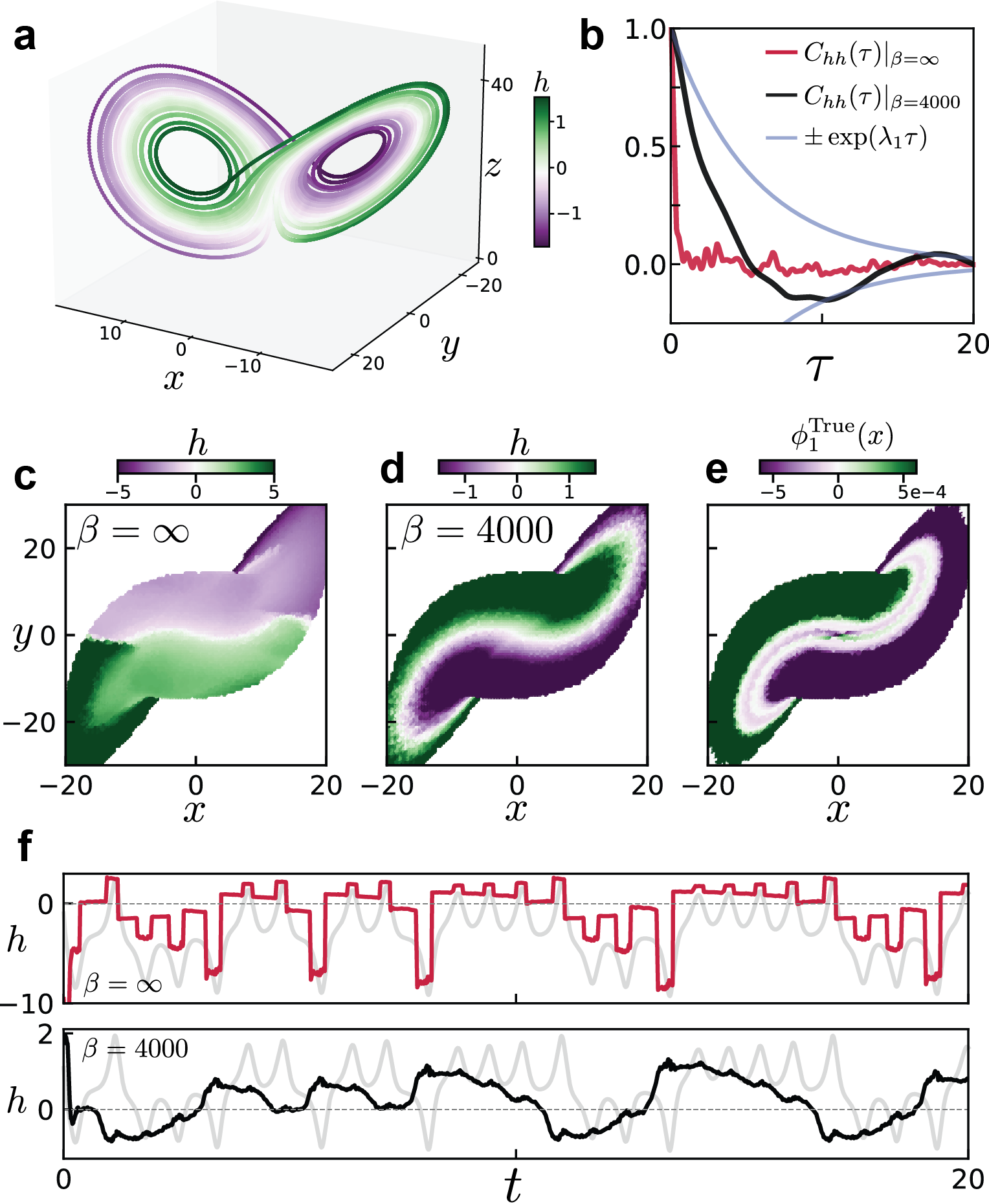
Figure S3: Variational IB discovers slow variables. (a) Variational IB applied to the Lorenz system. Color corresponds the encoding value $h_{t}$. (b) Time correlation functions of the encoded variable $C_{XY}(\tau)=\langle(X(\tau)-\bar{X})(Y(0)-\bar{Y})\rangle$ for high compression (black) and no compression (red). Blue shows the decay of the subleading Koopman eigenfunction using numerically-obtained eigenvalues. (c-d) Lorenz attractor projected onto the $x$-$y$ plane, colored by encoding variable. (e) Same projection, colored by the value of the true subleading Koopman eigenfunction. (f) Dynamics of $h_{t}$ obtained by encoding the state at every time during the true trajectory. Top corresponds to no compression ($\beta=\infty$), bottom corresponds to high compression ($\beta=4000$).

VIB for deterministic dynamics

IB is an inherently probabilistic framework. To handle deterministic dynamics, we make them effectively stochastic by introducing a stochastic sampling scheme. Concretely, rather than taking as our IB relevance variable $Y=X_{t+\Delta t}$, we take $Y=X_{t+\Delta t+\eta}$ where $\eta$ is a random uniformly-distributed time shift. Despite using a different relevance variable, this yields essentially the same optimal encoding as Eq. 7, where the eigenvalue $\text{e}^{\lambda_{n}\Delta t}$ is replaced by $\int d\eta\,p(\eta)\exp(\lambda_{n}(\Delta t+\eta))$. Crucially, the encoder retains its dependence on the transfer operator eigenfunctions $\phi_{n}(x)$ as before. In general, this need not be the case: selecting a new relevance variable changes the IB objective and will generically lead to a different encoder. Our choice of stochasticity which we introduce to the dynamics is chosen in such a way to preserve the form of the encoder.

We illustrate this with a prototypical example of deterministic chaotic dynamics, the Lorenz system [31]. In the steady state, the state variable of the Lorenz system resides on a chaotic attractor consisting of two “lobes” which encircle unstable fixed points (Fig. S3a). The encoding variable $h$ learned by VIB is the slowest varying function of the state $\bm{x}$, decaying as $\exp(\lambda^{\text{Re}}_{1}t)$ where $\lambda^{\text{Re}}_{1}$ is the real part of the first subleading eigenvalue of the transfer operator (here Perron-Frobenius operator) (Fig. S3b). Eigenvalues $\lambda_{n}$ as well as right eigenvectors $\phi_{n}(x)$ of the Perron-Frobenius operator were computed numerically using the Ulam method. The correspondence between $\phi_{1}(x)$ and $h$ disappears as $\beta$ is increased (Fig. S3c-e). The dynamics of $h$ also become notably less “slow”, and are instead nearly constant with occasional large jumps (Fig. S3f). This shows that in order for $h$ to be a valid slow variable, the compression term in Eq. (59) is crucial. These results are consistent with those obtained for exact IB, where we showed that the encoder incorporates the slow modes at low beta (high compression).

Appendix G Optimal encoding for Hopf normal form dynamics

We begin by deriving the Koopman generator in polar coordinates. In Cartesian coordinates, the equations of motion for the particle are

$$\dot{x} =(\mu-x^{2}-y^{2})x-\omega y$$ (60)

$$\dot{y} =(\mu-x^{2}-y^{2})y-\omega x$$ (61)

Expressed in polar coordinates, we have

$$f_{x}\hat{e}_{x} =f_{x}\cos\theta\hat{e}_{r}-f_{x}\sin\theta\hat{e}_{\theta}$$ (62)

$$f_{y}\hat{e}_{y} =f_{y}\sin\theta\hat{e}_{r}+f_{y}\cos\theta\hat{e}_{\theta}$$ (63)

From this we can compute $\mathcal{L}_{\mathcal{K}}\phi=f_{i}\partial_{i}\phi$,

$$f_{i}\partial_{i}\phi =(\partial_{r}\phi)(\mu-r^{2})r+\frac{1}{r}(\partial_{\theta}\phi)\omega r$$ (64)

$$=r(\mu-r^{2})(\partial_{r}\phi)+\omega\partial_{\theta}\phi$$ (65)

Because this differential equation is separable, we can find eigenfunctions by looking for eigenfunctions that are a function of either $r$ or $\theta$. Recall that for deterministic dynamics, a product of Koopman (generator) eigenfunctions is again an eigenfunction [19]. The eigenvalue equation for the radial coordinate is solved in Ref. [33], and in Ref. [65] it is shown that for this system there is no globally valid Koopman decomposition. However we are only interested in a subset of eigenfunctions, in particular those with eigenvalue with real part $\text{Re}\lambda_{i}\approx 0$, which may not suffice to approximate arbitrary functions of the state variable.

For the angle coordinate alone the situation is much simpler,

$$\omega\partial_{\theta}\phi(\theta)=\lambda\phi(\theta)$$

which is solved by functions $\phi_{n}(\theta)=\exp\left(\frac{\lambda_{n}}{\omega}\theta\right)$. Periodicity requires $\frac{\lambda}{\omega}2\pi=i2\pi n$, which leads to $\lambda=in\omega$. The eigenfunctions and eigenvalues are then

$$\phi_{n}(\theta)=e^{in\theta},\quad\quad\lambda_{n}=in\omega.$$

The corresponding eigenfunctions of the Perron-Frobenius operator are given by $\rho=\text{e}^{-in\theta}$.

We now consider an encoding $p(h|x)$.

$$p(h|r,\theta) \propto\exp\left\{\sum_{n}^{\infty}\text{e}^{\lambda_{n}\Delta t}\phi_{n}(r,\theta)\int r^{\prime}dr^{\prime}d\theta^{\prime}\rho_{n}(r^{\prime},\theta^{\prime})\log p(r^{\prime},\theta^{\prime}|h)\right\}$$ (66)

$$=\exp\left\{\sum_{n}^{\infty}\text{e}^{in\omega\Delta t}\int r^{\prime}dr^{\prime}d\theta^{\prime}\text{e}^{in(\theta-\theta^{\prime})}\log p(r^{\prime},\theta^{\prime}|h)\right\}+\mathcal{O}(e^{\text{Re}\lambda_{k}\Delta t})$$ (67)

where we retain only the eigenvalues with zero real part; the $\lambda_{k}$ in the above refer to those eigenvalues with non-zero real part. After neglecting these terms, it can be seen directly that $p(h|r,\theta)=p(h|\theta)$. The coordinates $(r^{\prime},\theta^{\prime})$ are used to denote $(r_{t+\Delta t},\theta_{t+\Delta t})$. The expression can be further simplified by replacing the sum over $n$ with a delta function, which leads to

$$p(h|r,\theta) \propto\exp\left\{\int r^{\prime}dr^{\prime}\log p(r^{\prime},(\theta+\omega\Delta t)|h)\right\}.$$ (68)

We next ask whether an encoder of the form $p(h|\theta)\propto\delta(h-\theta)$ is a solution. Recall that the probability distribution appearing in Eqn. 68 is a distribution over future positions, $p(R_{t+\Delta t}=r^{\prime},\Theta_{t+\Delta t}=\theta+\omega\Delta t|h)$. This distribution can be calculated as

$$p(r_{t+\Delta t},\theta_{t+\Delta t}|h) =\int rdrd\theta p(r_{t+\Delta t},\theta_{t+\Delta t}|r_{t},\theta_{t})p(r,\theta_{t}|h)$$ (69)

$$\propto\delta((\theta_{t+\Delta t}-\omega\Delta t)-h)$$ (70)

where we used that the two terms in the integrand of the first equation are both delta functions. Plugging this into Eqn. 68 shows that $p(h|\theta)\propto\delta(h-\theta)$ is consistent, and hence is an optimal encoding. In the presence of noise, the eigenvectors are perturbed and may gain a dependence on $r$ (see Fig. S4).

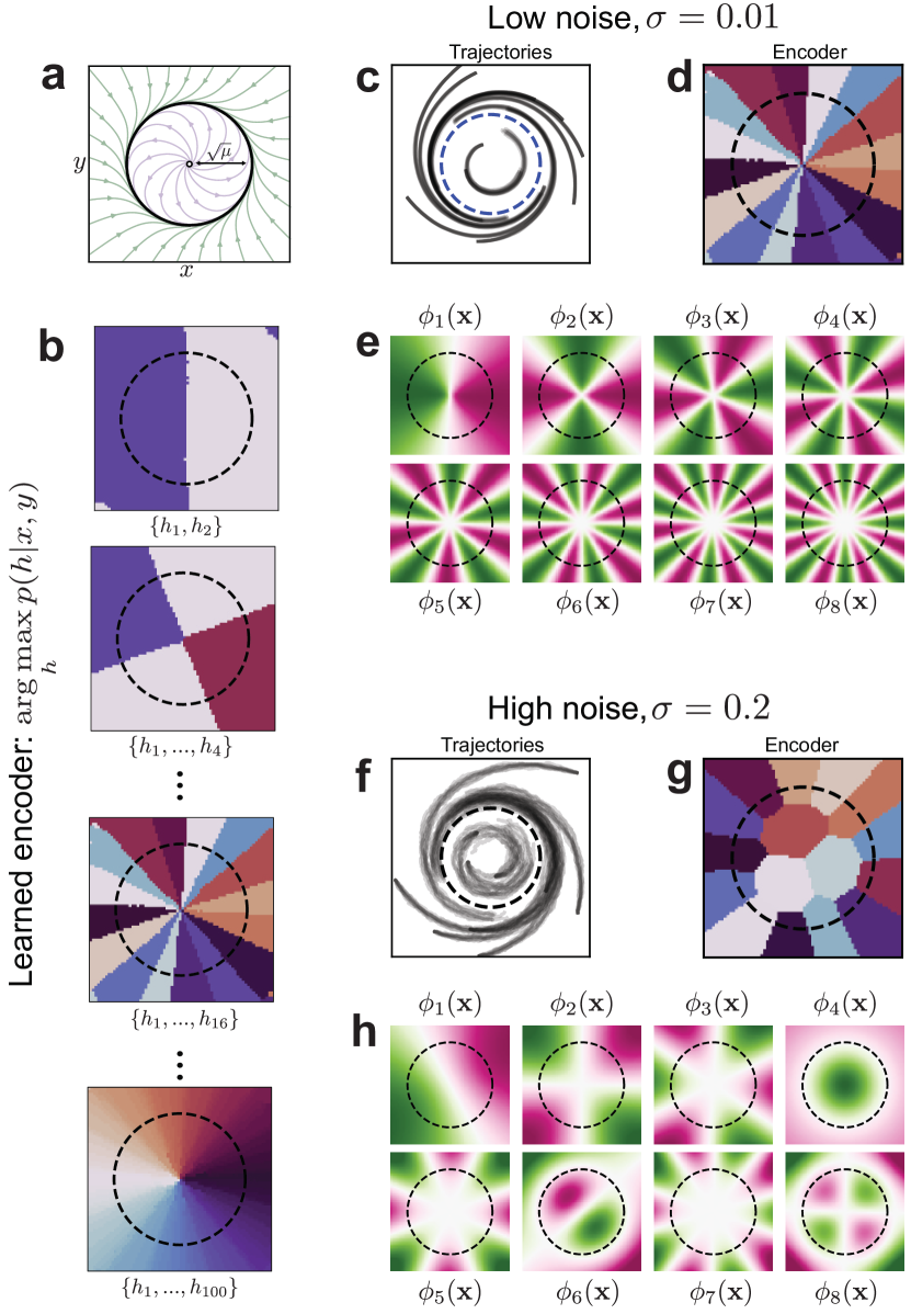
Figure S4: Eigenfunctions and IB partitions for the Hopf Oscillator. (a) Phase portrait for the deterministic Hopf oscillator. (b) Partitions found by IB for high beta but a restricted encoding alphabet $N_{H}$. (c) Example trajectories of the nearly deterministic Hopf oscillator, with small noise amplitude $\sigma=0.01$. (d) IB partition of the low noise dynamics for a $N_{H}=16$ encoding alphabet (same as appears in (b)). (e) For small noise, the first several eigenfunctions obtained numerically approximate the numerically expected ones of the form $\cos n\theta$. (f) Simulated trajectories of Hopf oscillator with higher noise amplitude $\sigma=0.2$. (g) IB partition of the low noise dynamics for a $N_{H}=16$ encoding alphabet; note the dependence on $r$. (h) The presence of noise changes the eigenfunctions, in particular they depend on $r$.

Appendix H VIB for fluid flow around a cylinder

Eigenfunction computation via dynamic mode decomposition

Here we provide some additional details on the computation used to generate components of Fig. 10. The true Koopman modes were computed using dynamical mode decomposition (DMD) [55, 56, 66]. DMD attempts to find a finite dimensional approximation of the Koopman operator using $n$ snapshots of the system’s state $x\in\mathbb{R}^{d}$ which are assembled into a data matrix $\mathbf{X}\in\mathbb{R}^{n\times d}$. One then attempts to find a linear evolution operator $K$ which propagates the state forward in time

$$\mathbf{X}_{t+\Delta t}=K\mathbf{X}_{t}.$$

The approximate Koopman operator is given by the least squares solution $K=\mathbf{X}_{t+\Delta t}\mathbf{X}_{t}^{+}$ where $\mathbf{X}_{t}^{+}$ denotes the pseudo-inverse of $\mathbf{X}_{t}$. Approximate Koopman eigenfunctions are given by $\phi_{n}(x)=x\cdot w_{n}$ where $w_{n}$ denotes the $n$th eigenvector of the matrix $K$ and is known as the $n$th DMD mode, denoted by $m^{(n)}$ in the main text.

Details on gradient analysis

As described in the main text, to understand to what extent VIB has learned the true eigenfunctions we analyze the gradients of the learned variables,

$$\frac{\partial h}{\partial v_{j}}=m^{(\text{IB})}_{j}+g_{\text{res},j}(\bm{v}(\bm{x})).$$ (71)

While it is unclear how to perform this decomposition in a general setting, we assume that the residual component $g_{\text{res},j}$ averages to zero over an oscillation period of the flow field $\bm{v}$. Then, $m^{(\text{IB})}_{j}\approx\langle\frac{\partial h}{\partial v_{j}}\rangle_{t}$ and $g_{\text{res},j}$ is given by variations about the mean. We see in Fig. S5 that these variations are much smaller than the mean in magnitude, and that they are essentially orthogonal to the mean vector. From this, we conclude that the gradients are given primarily by the constant part $\bm{m}$.

The learned latent functions vary for different training instances of the neural network. To extract the average gradient, we use PCA in an approach similar to that in Ref. [47]. The learned functions can have arbitrary sign structure; $h=h_{0}+ih_{1}$ is just as likely to be learned as $h=-h_{0}+ih_{1}$, for example. While in principle the network could learn arbitrary rotations, rather than simply changes in sign, we observe this is not the case. The distribution of gradients forms clusters in the high-dimensional gradient space corresponding to the four possible permutations of sign. PCA picks out the directions separating these clusters, as these are precisely the directions along which the data varies the most. This procedure gives an average gradient, while taking the varying sign structure into account. For reference, the gradient of a single instantiation of the VIB network can be seen in Fig. S6b.

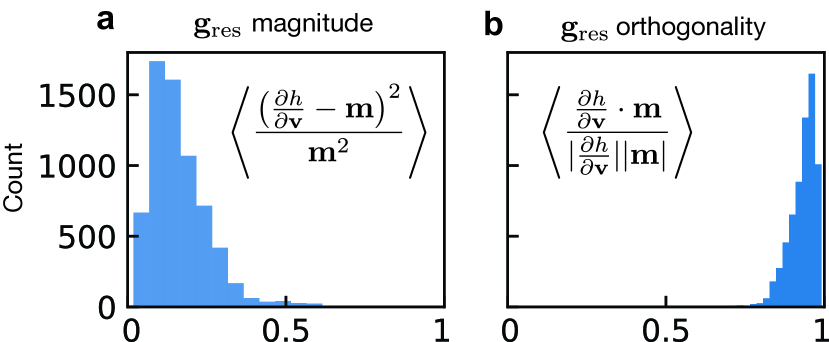
Figure S5: VIB gradients for fluid flow are nearly linear. We compare the linear part of the gradients of the VIB network to the residual which depends on the input field $\bm{v}(\bm{x})$. (a) The residual parts are smaller in magnitude than the linear part $\bm{m}$. Angle brackets denote average over space. (b) The residual parts are nearly orthogonal to the mean $\bm{m}$, as we see that the projection of the full gradient onto the mean is nearly 1.

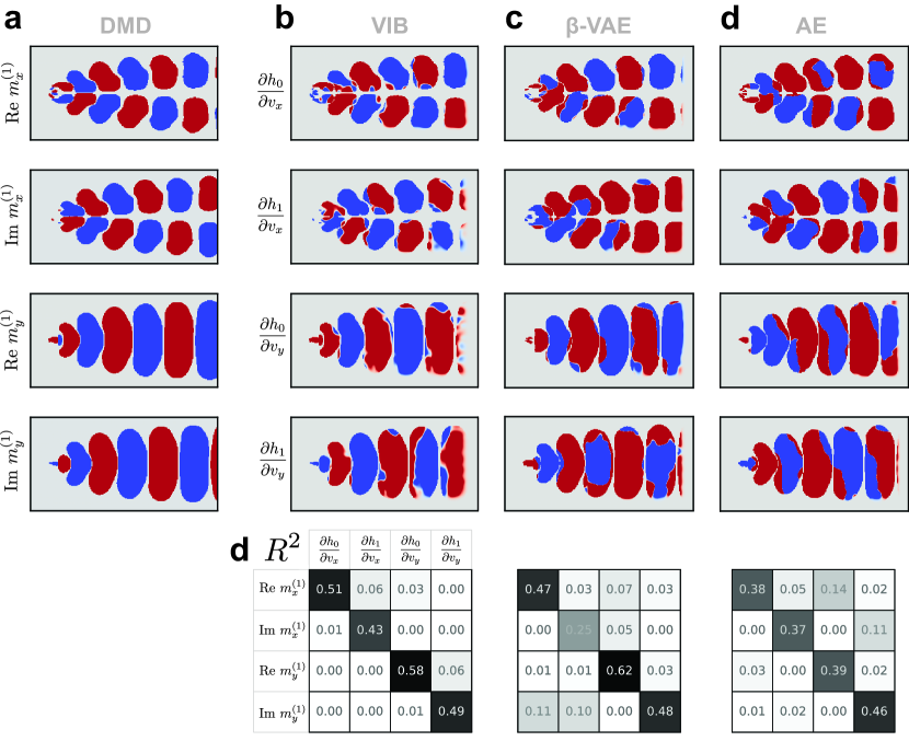
Figure S6: Learned latent variables for various deep neural networks. To compare latent variables we compare their gradients as in Fig. 10, which should correspond to Koopman modes. Here we show the gradients masked by regions in the DMD mode which have large amplitude. (a) True Koopman modes, with real and imaginary parts shown, obtained via DMD. (b) Corresponding modes for a VIB network. Matrix in the bottom row shows the $R^{2}$ values obtained by regressing the pixel values of the VIB gradients against the different components of the Koopman modes. (c) Corresponding modes for a $\beta$-variational autoencoder (VAE). The VAE has the same encoder structure as the VIB network, while the decoder has an inverted architecture to predict the future state $x_{t+\Delta t}$ from the latent variable $h_{t}$. Bottom row shows $R^{2}$ values, analogously to (b). (d) Corresponding modes for an autoencoder.

Appendix I Comment on VIB compared to other data-driven methods

Here we provide a brief overview of other data-driven methods for the learning of dynamical systems and model reduction.

Dynamic Mode Decomposition (DMD), in its original formulation [56, 55], attempts to find a finite dimensional approximation of the Koopman operator using $n$ snapshots of the system’s state $x\in\mathbb{R}^{d}$ which are assembled into a data matrix $\mathbf{X}\in\mathbb{R}^{n\times d}$. One then attempts to find a linear evolution operator $K$ which propagates the state forward in time

$$\mathbf{X}_{t+\Delta t}=K\mathbf{X}_{t}.$$

The approximate Koopman operator is given by the least squares solution $K=\mathbf{X}_{t+\Delta t}\mathbf{X}_{t}^{+}$ where $\mathbf{X}_{t}^{+}$ denotes the pseudo-inverse of $\mathbf{X}_{t}$. Approximate Koopman eigenfunctions are given by $\phi_{n}(x)=x\cdot w_{n}$ where $w_{n}$ denotes the $n$th eigenvector of the matrix $K$ and is known as the $n$th DMD mode.

DMD in its original formulation assumes that the Koopman operator linearly evolves the observed state variable. However, the true Koopman operator evolves arbitrary non-linear functions of the state variable forward in time. DMD has therefore been extended to account for non-linear functions through “extended DMD”, or eDMD [17]. eDMD augments the state vector with non-linear transformations of the state. As an example, a state vector $[-\bm{x}-]$ may be replaced by monomials $[-\bm{x}-,-\bm{x}^{2}-,-\bm{x}^{3}-]$ (where here we understand exponentiation as element-wise). Other approaches also exist, such as augmenting the state vector by several time-delayed state vectors [67]. Rather than constructing the full $d\times d$ matrix, where $d$ is the dimension of the (possibly augmented) state, one can directly construct a low-rank approximation of $K$ by computing the reduced-rank singular value decomposition (SVD) of the matrix $K$ from the SVDs of $\mathbf{X}_{t}$ and $\mathbf{X}_{t+\Delta t}$.

The primary limitation of DMD compared to VIB is the requirement that one first selects a suitable set of non-linear terms to account for potential non-linear eigenfunctions of the Koopman operator; it is unclear how to choose this set of functions in a generic setting.

Diffusion Maps refer to a technique which attempts to approximate the Perron-Frobenius operator, or rather the integral kernel $p(x_{t+\Delta t}|x_{t})$ [14, 68]. Given this approximation, one computes eigenfunctions and uses them as a low-dimensional parameterization of the data (“diffusion coordinates”).

This method takes data pairs $\{x^{(i)}_{t},x^{(i)}_{t+\Delta t}\}_{i}$ and approximates the probability of observing these two points via a kernel $p(x^{(i)}_{t},x^{(j)}_{t+\Delta t})\approx k(x^{(i)}_{t},x^{(j)}_{t+\Delta t})$, where one typically takes a Gaussian Ansatz

$$k_{\epsilon}(x,y)\propto\exp\left[\frac{-(x-y)^{2}}{\epsilon}\right].$$

From this, one can assemble the conditional probability distributions into a matrix

$$P_{ij}=p(x^{(j)}_{t+\Delta t}|x^{(i)}_{t})=\frac{p(x^{(i)}_{t},x^{(j)}_{t+\Delta t})}{p(x^{(i)}_{t})}=\frac{k(x^{(i)}_{t},x^{(j)}_{t+\Delta t})}{\sum_{j}k(x^{(i)}_{t},x^{(j)}_{t+\Delta t})}.$$

This matrix describes the evolution of probability distributions on a graph where each node is a data point. In practice, a symmetrized version of $P$ is constructed and the learned eigenvectors are adjusted after the diagonalization [14, 68]. To compute the diffusion coordinates of an arbitrary point that wasn’t in the original dataset, one inverts the definition of the adjoint transfer operator eigenfunction

$$\phi_{i}(\bm{x}_{\text{new}})\approx\frac{1}{\lambda_{i}}\sum_{k}P^{\dagger}_{jk}\phi_{i}(\bm{x}_{k})$$

where $\lambda_{i}$ is the $i$-th eigenvalue.

Diffusion maps have the advantage, relative to DMD, that they find the full Perron-Frobenius operator and not a linear approximation to it. However, while DMD can isolate the dominant eigenvectors of the operator using reduced-rank SVD, it is less clear how they can be extracted with diffusion maps without first computing the full matrix $P$. We note that VIB, like DMD, also directly learns the dominant modes and does not require estimation of the full transfer operator.

(Variational) Autoencoders belong to a class of deep learning methods used for model reduction. Autoencoders are composed of an encoder which compresses the observable $\bm{x}$ into a lower-dimensional latent variable $\bm{z}$, and a decoder which attempts to reconstruct the original state $\bm{x}$. Variational autoencoders aim to learn a probability distribution over observations $p_{\theta}(\bm{x})\approx p(\bm{x})$ from which one can directly sample [69]. This is done by assuming that the latent variable is low dimensional, and optimizing the objective

$$\mathcal{L}_{\beta\text{-VAE}}=\mathbb{E}_{q_{\phi}(z|x)}[-\log p_{\theta}(x|z)]-\beta D_{\text{KL}}(q(z|x)\lVert\hat{p}(z))$$

where $q_{\phi}(z|x)$ is the posterior on the latent variables $z$ and is parameterized by a neural network (encoder) with parameters $\phi$, and $p_{\theta}(x|z)$ denotes the decoding network with parameters $\theta$. Strictly speaking, we present in the above objective function the $\beta$-VAE loss [59]. With $\beta=1$, which is the case for the original VAE [69], the objective is an upper bound on the log likelihood $-\mathbb{E}[\log p_{\theta}(x)]$ which is minimized when $p_{\theta}(x)$ is equal to the true data distribution $p(x)$. The term $\beta$ controls compression as in the IB objective, however it has the opposite effect: small $\beta_{\text{IB}}$ corresponds to high compression, while small $\beta_{\text{VAE}}$ corresponds to low compression.

In cases where one directly computes the probabilities $p_{\theta}(x|z)$ the first term can be evaluated directly, else it is typically replaced with an $L_{2}$ loss $\lVert x-g_{\theta}(z)\lVert^{2}$ (where $g_{\theta}$ is a deterministic neural network), which is equivalent to assuming a Gaussian Ansatz for $p_{\theta}$ with a fixed variance.

The VIB loss function is very similar to the $\beta$-VAE loss [70]. Rather than attempting to reconstruct the original state $x$, VIB replaces this term with an estimate of the mutual information between the latent variable $z$ and some other relevance variable $y$ (for us, $y=x_{t+\Delta t}$). In contrast to DMD and diffusion maps, neither VIB nor $\beta$-VAEs make any mention of transfer operators and are instead motivated by purely statistical considerations. As we show in the main text, the latent variables learned by VIB correspond to eigenfunctions of the transfer operator. While we cannot claim that that $\beta$-VAEs learn the same thing, some preliminary results in Fig. S6 suggest they may coincide to some degree.

Other neural networks can also be used for model reduction. For example, [21] uses recurrent neural networks (RNNs) to learn the evolution of macroscopic variables. To ensure stability and fidelity, the macroscopic variables are periodically “lifted” to the full microscopic state, which is then evolved for several time steps to recalibrate the RNN’s hidden state. While interpretability of the latent variables has yet to be explored in such models, we expect the addition of VIB-like objective functions may aid interpretability without harming performance.

As another example, [20] attempts to learn the full Koopman operator using neural networks. This can be thought of as an extension of eDMD, where instead of prescribing the library of nonlinear terms by hand, they can be learned by a neural network. The latent dynamics are then encouraged to be linear by minimizing the deviation between the true future (latent) state $\bm{z}_{t+\Delta t}$ and its linear approximation found by least squares. This approach was applied primarily to deterministic systems. We expect that combining their method of encouraging linear latent dynamics together with the VIB objective function may be fruitful and lead to more well-behaved latent variables.

Appendix J Simulation Parameters

Triple well simulations For the dynamics of the triple well we work directly with the force $F=-\partial_{x}U$,

$$F(x) =\frac{-1}{200}\left(9375x^{5}-7500x^{3}+1100x-20\right).$$

The evolution of the Brownian particle’s position $x_{t}$ is given by

$$\text{d}x_{t}=\frac{F(x_{t})}{\gamma}\text{d}t+\sigma\sqrt{\text{d}t}\eta_{t}$$ (72)

where $\eta_{t}$ is white noise with unit variance. The noise magnitude $\sigma$ is related to the diffusion constant in Eq. 19 by $D=\frac{\sigma^{2}}{2}$. We use $\sigma=1.0$ and $\gamma=0.2$

Simulations were performed with $N_{\text{init}}=10^{5}$ initial conditions, with 300 trajectories generated from each initial condition. The state is evolved for $100$ steps at $\text{d}t=2\cdot 10^{-3}$. The transfer matrix is approximated by binning the space $x\in[-1,1]$ with $N_{\text{bins}}=100$ bins. IB is performed using a time delay $\Delta t=64$ steps.

Pitchfork bifurcation simulations The system was evolved according to the stochastic differential equation Eq. 72 with $F(x)=-\mu x-x^{3}$, $\gamma=1$ and $\sigma=0.1$. For each value of $\mu$, $10^{5}$ initial conditions were simulated with 2000 trajectories starting at each initial condition. These were evolved for 100 time steps of $\text{d}t=2\cdot 10^{-3}$.

Hopf oscillator simulations The system was evolved according to Eq. 72 with the force given by Eq.11 in the main text, with $\gamma=1$ and $\sigma=10^{-2}$, $\omega=4.0$ and $\mu=0.25$. For each value of $\mu$, $10^{6}$ initial conditions were simulated with 1000 trajectories starting at each initial condition. These were evolved for 50 time steps of $\text{d}t=2\cdot 10^{-3}$.

Lorenz system simulations The system was evolved according to

$$\dot{x} =\sigma(y-x)$$ (73)

$$\dot{y} =x(\rho-z)-y$$ (74)

$$\dot{z} =xy-\beta z$$ (75)

with $\rho=28$, $\beta=8/3$ and $\sigma=10$. We took $10^{3}$ initial conditions from which trajectories were simulated for $10^{5}$ steps with $\text{d}t=2\cdot 10^{-3}$. We compute the true eigenfunctions using the GAIO library [71].

Fluid flow simulations The fluid flow simulations simulations are contained in the “Cylinder in Crossflow” dataset, downloaded from Ref. [72]. We take the dataset at Reynolds number 150, and interpolate the velocity field from the unstructured 6569-node mesh to a regular grid of $300\times 150$ pixels. The VIB networks are trained with $\beta=10^{7}$ and a time buffer $\Delta t$ chosen randomly between $[4,24]$ (see our comment on time randomization in “VIB for deterministic dynamics” in Appendix F).

References

- Kuramoto [1984] Y. Kuramoto, Chemical Oscillations, Waves, And Turbulence (Springer, 1984).
- Haken [1983] H. Haken, Synergetics: An Introduction, Springer Series in Synergetics (Springer Berlin Heidelberg, 1983).
- Pavliotis and Stuart [2010] G. Pavliotis and A. Stuart, Multiscale Methods: Averaging and Homogenization, Texts in Applied Mathematics (Springer New York, 2010).
- Givon et al. [2004] D. Givon, R. Kupferman, and A. Stuart, Nonlinearity 17, R55–R127 (2004).
- Kuramoto and Nakao [2019] Y. Kuramoto and H. Nakao, Philosophical Transactions of the Royal Society A: Mathematical, Physical and Engineering Sciences 377, 20190041 (2019).
- Kunihiro et al. [2022] T. Kunihiro, Y. Kikuchi, and K. Tsumura, Geometrical Formulation of Renormalization-Group Method as an Asymptotic Analysis: With Applications to Derivation of Causal Fluid Dynamics, Fundamental Theories of Physics (Springer Nature Singapore, 2022).
- Kuramoto [1989] Y. Kuramoto, Progress of Theoretical Physics Supplement 99, 244–262 (1989).
- Mori and Kuramoto [1998] H. Mori and Y. Kuramoto, Dissipative Structures and Chaos , 93–117 (1998).
- Chen et al. [1996] L.-Y. Chen, N. Goldenfeld, and Y. Oono, Physical Review E 54, 376–394 (1996).
- Chapman and Cowling [1990] S. Chapman and T. G. Cowling, The mathematical theory of non-uniform gases: an account of the kinetic theory of viscosity, thermal conduction and diffusion in gases (Cambridge university press, 1990).
- Otto and Rowley [2021] S. E. Otto and C. W. Rowley, Annual Review of Control, Robotics, and Autonomous Systems 4, 59–87 (2021).
- Klus et al. [2018] S. Klus, F. Nüske, P. Koltai, H. Wu, I. Kevrekidis, C. Schütte, and F. Noé, Journal of Nonlinear Science 28, 985 (2018).
- Brunton et al. [2020] S. L. Brunton, B. R. Noack, and P. Koumoutsakos, Annual Review of Fluid Mechanics 52, 477 (2020), https://doi.org/10.1146/annurev-fluid-010719-060214 .
- Coifman and Lafon [2006] R. R. Coifman and S. Lafon, Applied and Computational Harmonic Analysis 21, 5 (2006), special Issue: Diffusion Maps and Wavelets.
- Jain and Haller [2021] S. Jain and G. Haller, Nonlinear Dynamics 107, 1417–1450 (2021).
- Cenedese et al. [2022] M. Cenedese, J. Axås, B. Bäuerlein, K. Avila, and G. Haller, Nature Communications 13, 10.1038/s41467-022-28518-y (2022).
- Williams et al. [2015] M. O. Williams, I. G. Kevrekidis, and C. W. Rowley, Journal of Nonlinear Science 25, 1307 (2015).
- Mezić [2005] I. Mezić, Nonlinear Dynamics 41, 309–325 (2005).
- Brunton et al. [2022] S. L. Brunton, M. Budišić, E. Kaiser, and J. N. Kutz, SIAM Review 64, 229 (2022).
- Takeishi et al. [2017] N. Takeishi, Y. Kawahara, and T. Yairi, in Advances in Neural Information Processing Systems, Vol. 30, edited by I. Guyon, U. V. Luxburg, S. Bengio, H. Wallach, R. Fergus, S. Vishwanathan, and R. Garnett (Curran Associates, Inc., 2017).
- Vlachas et al. [2022] P. R. Vlachas, G. Arampatzis, C. Uhler, and P. Koumoutsakos, Nature Machine Intelligence 4, 359 (2022).
- Wu et al. [2022] T. Wu, T. Maruyama, and J. Leskovec, Learning to accelerate partial differential equations via latent global evolution (2022), arXiv:2206.07681 [cs.LG] .
- Cvitanović and Lippolis [2012] P. Cvitanović and D. Lippolis, AIP Conference Proceedings 10.1063/1.4745574 (2012).
- Jayant et al. [1993] N. Jayant, J. Johnston, and R. Safranek, Proceedings of the IEEE 81, 1385 (1993).
- Creutzig and Sprekeler [2008] F. Creutzig and H. Sprekeler, Neural Computation 20, 1026 (2008).
- Tishby et al. [2000] N. Tishby, F. C. Pereira, and W. Bialek, The information bottleneck method (2000), arXiv:physics/0004057 [physics.data-an] .
- Creutzig et al. [2009] F. Creutzig, A. Globerson, and N. Tishby, Phys. Rev. E 79, 041925 (2009).
- Cover and Thomas [2012] T. Cover and J. Thomas, Elements of Information Theory (Wiley, 2012).
- Lasota and Mackey [1998] A. Lasota and M. C. Mackey, Chaos, Fractals, and Noise (Springer, 1998) p. 492.
- Alemi et al. [2017] A. A. Alemi, I. Fischer, J. V. Dillon, and K. Murphy, in International Conference on Learning Representations (2017).
- Lorenz [1963] E. N. Lorenz, Journal of the Atmospheric Sciences 20, 130–141 (1963).
- Note [1] The essential spectrum is defined as the part of the spectrum that is not the discrete spectrum. Here, we assume that the essential radius of (the maximum absolute value of eigenvalues in the essential spectrum) is small enough compared to the first few eigenvalues in the point spectrum so that, for these eigenvalues, and the corresponding terms can be neglected. This is not always the case; we focus on cases where this assumption holds.
- Gaspard et al. [1995] P. Gaspard, G. Nicolis, A. Provata, and S. Tasaki, Phys. Rev. E 51, 74 (1995).
- Froyland [2013] G. Froyland, Physica D: Nonlinear Phenomena 250, 1 (2013).
- Parker et al. [2002] A. Parker, T. v. Gedeon, and A. Dimitrov, in Advances in Neural Information Processing Systems, Vol. 15, edited by S. Becker, S. Thrun, and K. Obermayer (MIT Press, 2002).
- Wu et al. [2020] T. Wu, I. Fischer, I. L. Chuang, and M. Tegmark, in Proceedings of The 35th Uncertainty in Artificial Intelligence Conference, Proceedings of Machine Learning Research, Vol. 115, edited by R. P. Adams and V. Gogate (PMLR, 2020) pp. 1050–1060.
- Chechik et al. [2005] G. Chechik, A. Globerson, N. Tishby, and Y. Weiss, Journal of Machine Learning Research 6, 165 (2005).
- Ngampruetikorn and Schwab [2021] V. Ngampruetikorn and D. J. Schwab, in Advances in Neural Information Processing Systems, edited by A. Beygelzimer, Y. Dauphin, P. Liang, and J. W. Vaughan (2021).
- Palmer et al. [2015] S. E. Palmer, O. Marre, M. J. Berry, and W. Bialek, Proceedings of the National Academy of Sciences 112, 6908 (2015).
- Sachdeva et al. [2021] V. Sachdeva, T. Mora, A. M. Walczak, and S. E. Palmer, PLOS Computational Biology 17, 1 (2021).
- Chu and Voth [2007] J.-W. Chu and G. A. Voth, Biophysical Journal 93, 3860 (2007).
- Ulam [1960] S. Ulam, Problems in Modern Mathematics (Science Editions, 1960).
- Li [1976] T.-Y. Li, Journal of Approximation Theory 17, 177 (1976).
- Shaw [1981] R. Shaw, Zeitschrift für Naturforschung A 36, 80–112 (1981).
- Crutchfield and Packard [1983] J. Crutchfield and N. Packard, Physica D: Nonlinear Phenomena 7, 201–223 (1983).
- Froyland [2005] G. Froyland, Physica D: Nonlinear Phenomena 200, 205 (2005).
- Gökmen et al. [2021a] D. E. Gökmen, Z. Ringel, S. D. Huber, and M. Koch-Janusz, Phys. Rev. Lett. 127, 240603 (2021a).
- Gökmen et al. [2021b] D. E. Gökmen, Z. Ringel, S. D. Huber, and M. Koch-Janusz, Phys. Rev. E 104, 064106 (2021b).
- Gökmen et al. [2023] D. E. Gökmen, S. Biswas, S. D. Huber, Z. Ringel, F. Flicker, and M. Koch-Janusz, Compression theory for inhomogeneous systems (2023), arXiv:2301.11934 [cond-mat.stat-mech] .
- van den Oord et al. [2019] A. van den Oord, Y. Li, and O. Vinyals, Representation learning with contrastive predictive coding (2019), arXiv:1807.03748 [cs.LG] .
- Strogatz [2018] S. H. Strogatz, Nonlinear Dynamics and Chaos (CRC Press, 2018) p. 532.
- Albright [@jacobalbright3585] J. Albright (@jacobalbright3585), Flow Visualization in a Water Channel, https://www.youtube.com/watch?v=30_aADFVL9M (2017), [Accessed 03-Sept-2023].
- @NOAASatellites [2021] @NOAASatellites, Earth from Orbit: von Kármán Vortices, https://www.youtube.com/watch?v=SawKLWT1bDA (2021), [Accessed 03-Sept-2023].
- Tencer and Potter [2020] J. Tencer and K. Potter, A tailored convolutional neural network for nonlinear manifold learning of computational physics data using unstructured spatial discretizations (2020), arXiv:2006.06154 [physics.comp-ph] .
- Rowley et al. [2009] C. W. Rowley, I. Mezić, S. Bagheri, P. Schlatter, and D. S. Henningson, Journal of Fluid Mechanics 641, 115–127 (2009).
- Schmid [2010] P. J. Schmid, Journal of Fluid Mechanics 656, 5–28 (2010).
- Gordon et al. [2021] A. Gordon, A. Banerjee, M. Koch-Janusz, and Z. Ringel, Phys. Rev. Lett. 126, 240601 (2021).
- Slonim [2002] N. Slonim, The Information Bottleneck: Theory and Applications, Ph.D. thesis, Hebrew University of Jerusalem (2002), retrieved from https://www.cs.huji.ac.il/labs/learning/Theses/Slonim_PhD.pdf.
- Higgins et al. [2017] I. Higgins, L. Matthey, A. Pal, C. Burgess, X. Glorot, M. Botvinick, S. Mohamed, and A. Lerchner, in International Conference on Learning Representations (2017).
- Mikhaeil et al. [2022] J. Mikhaeil, Z. Monfared, and D. Durstewitz, in Advances in Neural Information Processing Systems, Vol. 35, edited by S. Koyejo, S. Mohamed, A. Agarwal, D. Belgrave, K. Cho, and A. Oh (Curran Associates, Inc., 2022) pp. 11297–11312.
- Koppe et al. [2019] G. Koppe, H. Toutounji, P. Kirsch, S. Lis, and D. Durstewitz, PLOS Computational Biology 15, 1 (2019).
- Gilpin [2020] W. Gilpin, in Advances in Neural Information Processing Systems, Vol. 33, edited by H. Larochelle, M. Ranzato, R. Hadsell, M. Balcan, and H. Lin (Curran Associates, Inc., 2020) pp. 204–216.
- Eivazi et al. [2022] H. Eivazi, S. Le Clainche, S. Hoyas, and R. Vinuesa, Expert Systems with Applications 202, 117038 (2022).
- Rolinek et al. [2019] M. Rolinek, D. Zietlow, and G. Martius, in Proceedings of the IEEE/CVF Conference on Computer Vision and Pattern Recognition (CVPR) (2019).
- Page and Kerswell [2019] J. Page and R. R. Kerswell, Journal of Fluid Mechanics 879, 1–27 (2019).
- Tu et al. [2014] J. H. Tu, C. W. Rowley, D. M. Luchtenburg, S. L. Brunton, and J. N. Kutz, Journal of Computational Dynamics 1, 391 (2014).
- Brunton et al. [2017] S. L. Brunton, B. W. Brunton, J. L. Proctor, E. Kaiser, and J. N. Kutz, Nature Communications 8, 19 (2017).
- Coifman et al. [2008] R. R. Coifman, I. G. Kevrekidis, S. Lafon, M. Maggioni, and B. Nadler, Multiscale Modeling & Simulation 7, 842 (2008), https://doi.org/10.1137/070696325 .
- Kingma and Welling [2022] D. P. Kingma and M. Welling, Auto-encoding variational bayes (2022), arXiv:1312.6114 [stat.ML] .
- Burgess et al. [2018] C. P. Burgess, I. Higgins, A. Pal, L. Matthey, N. Watters, G. Desjardins, and A. Lerchner, Understanding disentangling in -vae (2018), arXiv:1804.03599 [stat.ML] .
- Dellnitz et al. [2001] M. Dellnitz, G. Froyland, and O. Junge, in Ergodic Theory, Analysis, and Efficient Simulation of Dynamical Systems, edited by B. Fiedler (Springer Berlin Heidelberg, Berlin, Heidelberg, 2001) pp. 145–174.
- Tencer [2020] J. Tencer, Cylinder in Crossflow (2020).