Promoting Counterfactual Robustness through Diversity

Abstract

Counterfactual explanations shed light on the decisions of black-box models by explaining how an input can be altered to obtain a favourable decision from the model (e.g., when a loan application has been rejected). However, as noted recently, counterfactual explainers may lack robustness in the sense that a minor change in the input can cause a major change in the explanation. This can cause confusion on the user side and open the door for adversarial attacks. In this paper, we study some sources of non-robustness. While there are fundamental reasons for why an explainer that returns a single counterfactual cannot be robust in all instances, we show that some interesting robustness guarantees can be given by reporting multiple rather than a single counterfactual. Unfortunately, the number of counterfactuals that need to be reported for the theoretical guarantees to hold can be prohibitively large. We therefore propose an approximation algorithm that uses a diversity criterion to select a feasible number of most relevant explanations and study its robustness empirically. Our experiments indicate that our method improves the state-of-the-art in generating robust explanations, while maintaining other desirable properties and providing competitive computational performance.

1 Introduction

Counterfactual explanations support the outcome of a black-box machine learning model by explaining how the input could be changed to produce a different decision (Guidotti et al. 2019; Karimi et al. 2023; Stepin et al. 2021; Wachter, Mittelstadt, and Russell 2017). Roughly speaking, a counterfactual explainer is called robust, if a minor change in the input cannot cause a major change in the explanation. The actual change can be quantified, for example, by the Euclidean distance, by the number of features that have to be changed or by a cost associated with changing the features. One motivation for robustness is user justifiability. Two similar users would expect to get a similar explanation and an individual user may be surprised if a minor change in its characteristics would result in a completely different explanation (Hancox-Li 2020). Robustness is also relevant from a fairness perspective because some non-robust counterfactual explainers can be manipulated such that they offer better explanations for particular subgroups (Slack et al. 2021).

There are different reasons for non-robustness. As noted in (Slack et al. 2021), local search methods as hill-climbing can be highly sensitive to input perturbations and may therefore not be robust. All heuristic methods can be susceptible to such problems, in particular if they rely on randomization. However, as noted in (Fokkema, de Heide, and van Erven 2022), there are more fundamental problems that can cause robustness problems. Intuitively, whenever an input is between two decision boundaries on opposite sides, a minor change in the input can result in a major change in the computed counterfactual. We illustrate this in Figure 1 for two different decision boundaries and give additional explanations in the caption. Note that this problem even applies to exact methods.

Figure 1: The figure shows the decision boundaries of two classes $B$ (blue outer region) and $Y$ (yellow inner region) in two scenarios (left, right). In both cases, the points $x$, $x_{1}$, $x_{2}$ are relatively close, but their corresponding counterfactuals $\mathbf{c},\mathbf{c}_{1},\mathbf{c}_{2}$ on the decision boundary are relatively far away from each other wrt. Euclidean distance.

The problem in Figure 1 occurs if the input $x$ is close to the center between decision boundaries. Clearly, a counterfactual explainer that returns a single counterfactual is bound to lack robustness in such a scenario. One intuitive idea to overcome this fundamental problem is to report multiple counterfactuals instead of a single one. In Section 4, we study this idea theoretically and identify some interesting cases under which an exhaustive explainer can guarantee robustness by returning all approximate counterfactuals with respect to some tolerance parameter $\epsilon$. Unfortunately, the exhaustive explainer is not practically viable because the number of identified counterfactuals can be prohibitively large or even infinite. The blowup is partially caused by sets of counterfactuals that are redundant in the sense that they are all very similar. Reporting all of them is not desirable from an explanation perspective (because the explanation becomes too large) and is, indeed, not always necessary for guaranteeing robustness. To overcome these issues, we propose an approximation algorithm in Section 5 that incrementally builds up a set of counterfactuals while filtering new candidates based on a diversity criterion. In Section 6, we study the robustness and general performance of our approximation algorithm and compare it to DiCE (Mothilal, Sharma, and Tan 2020), a state-of-the-art algorithm to generate sets of diverse explanations. Our experiments show that our algorithm is more robust and also outperforms DiCE along other metrics of interest, while maintaining superior runtime performance.

2 Related Work

Counterfactual explanations and their properties. Several approaches have been proposed to compute counterfactual explanations for learning models. The seminal work of Wachter et al (Wachter, Mittelstadt, and Russell 2017) used gradient-based optimisation to generate counterfactual explanations for neural networks. These counterfactuals are obtained by optimising a loss function that encourages their validity (i.e., the counterfactual flips the classification outcome of the network) and proximity (i.e., the counterfactual is close to the original input for which the explanation is sought under some distance metric). Following this initial proposal, other approaches have been developed to enforce additional properties on the explanations they produce. For instance, DiCE (Mothilal, Sharma, and Tan 2020) proposed novel loss terms to generate sets of counterfactual explanations for a given input. By maximising the diversity within the set, the authors provide a method to better approximate local decision boundaries of machine learning models, thus improving the explanatory power of counterfactuals. A different approach is proposed in proto (Van Looveren and Klaise 2021), where the authors present a method to generate counterfactual explanations that lie in the data manifold of the dataset in an attempt to improve their plausiblity. The method relies on class prototypes identified by variational auto-encoders or kd-trees to guide the search for high-quality explanations. Moving away from continuous optimisation techniques for differentiable models, (Mohammadi et al. 2021) cast the problem of finding counterfactual explanations as a constrained optimisation problem encoded and solved using Mixed-Integer Linear Programming. Similarly, FACE (Karimi et al. 2020) uses Satisfiability Modulo Theory solving to derive a model-agnostic counterfactual explanation algorithm. For further details on counterfactual explanations we refer to (Karimi et al. 2023), which offers a recent survey on the state of the art in this area.

Robustness and explainability. As explanations are increasingly used to guide decisions in areas with clear societal implications (ProPublica 2016; FICO Community 2019), their reliability has come under scrutiny. In particular, recent work has highlighted issues related to the robustness of state-of-the-art counterfactual explainers. For instance, (Upadhyay, Joshi, and Lakkaraju 2021; Black, Wang, and Fredrikson 2022; Jiang et al. 2023) study how the validity of counterfactual explanations is affected when the weights of a neural network are slightly altered, e.g., due to retraining or fine-tuning, observing that many state-of-the-art approaches fail to generate robust counterfactuals in this setting. Robustness to model changes is also investigated in (Dutta et al. 2022), where the authors consider tree-based classifiers and propose a statistical procedure to test the robustness of counterfactual explanations when minor modifications are applied to the tree. A related notion of robustness is also studied in (Leofante, Botoeva, and Rajani 2023; Pawelczyk, Broelemann, and Kasneci 2020), where the authors consider the more general setting of robustness under model multiplicity.

In another line of work, (Leofante and Lomuscio 2023) show that the validity of a counterfactual explanation may be compromised by adversarial perturbations directly applied to the explanation itself. The authors discuss how such lack of model robustness (as opposed to input robustness as we consider here) hinder a transparent interaction between humans and AI agents. The authors propose to use formal verification techniques to counter this problem and derive a method to rigorously quantify the robustness of the explanations they produce. The same notion of robustness is also addressed in (Pawelczyk et al. 2023), where a probabilistic method is proposed to generate robust counterfactuals.

To the best of our knowledge, the only existing work that aims at improving input robustness is (Slack et al. 2021). In particular, they showed that algorithms based on gradient search can be highly sensitive to changes in the input and may thus result in radically different explanations for very similar events. While they offer useful empirical observations on how to circumvent this robustness issue, they do not propose an algorithm to generate counterfactuals that are robust. In this paper we fill this gap and propose to move away from instance-based explanations and instead report multiple, diverse counterfactuals to improve the robustness of counterfactual explanations.

3 Background

We focus on classification problems over tabular data. Our datasets are defined by a set of feature variables (features) $X_{1},\dots,X_{k}$ and a class variable $C$. We let $D_{1},\dots,D_{k}$ denote the domains associated with the variables and $L$ denote the class labels associated with the class $C$. We let $\mathcal{D}=\bigtimes_{i=1}^{k}D_{i}$ denote the set of all inputs (of the classification problem). A domain $D$ is called discrete if $D$ is countable and continuous if $D$ is an uncountable subset of $\mathbb{R}$. A classification problem $P=((D_{1},\dots,D_{k}),L,E)$ consists of domains, class labels and a set of training examples $E=\{(\mathbf{x}_{i},y_{i})\mid 1\leq i\leq N,\mathbf{x}_{i}\in\mathcal{D},y_{i}\in L\}$. A training example $(\mathbf{x}_{i},y_{i})$ consist of an instantiation $\mathbf{x}_{i}$ of the variables and a class label $y_{i}$. A classifier is a function $\operatorname{Cl}:\mathcal{D}\rightarrow L$ that assigns a class label $l\in L$ to every input $\mathbf{x}$.

Counterfactual explanations explain how an input can be changed to change the classification outcome. For example, in a loan application scenario, users may be interested in learning what they have to change in order to be successful. Formally, given a classifier $\operatorname{Cl}$ and an input $\mathbf{x}\in\mathcal{D}$ such that $\operatorname{Cl}(\mathbf{x})=y$, a counterfactual explanation is an input $\mathbf{c}\in\mathcal{D}$ such that $\operatorname{Cl}(\mathbf{c})\neq y$ and $\mathbf{c}$ is close to $\mathbf{x}$. Proximity can be defined by different measures. This includes metrics like Euclidean or Manhattan distance, weighted variants and measures that count the number of features that change. Given one such distance measure $d:\mathcal{D}\times\mathcal{D}\rightarrow\mathbb{R}_{0}^{+}$, a point $\mathbf{x}^{\prime}\in\mathcal{D}$ may satisfy the proximity constraint if it minimizes the distance among all points that take a different class label or if the distance is below a particular threshold. Unless stated otherwise, we do not make any assumptions about $d$ other than that it is non-negative. Often, $d$ will be a metric, that is, it will also satisfy

Definiteness:

$d(\mathbf{x}_{1},\mathbf{x}_{2})=0$ if and only if $\mathbf{x}_{1}=\mathbf{x}_{2}$.

Symmetry:

$d(\mathbf{x}_{1},\mathbf{x}_{2})=d(\mathbf{x}_{2},\mathbf{x}_{1})$.

Triangle Inequality:

$d(\mathbf{x}_{1},\mathbf{x}_{3})\leq d(\mathbf{x}_{1},\mathbf{x}_{2})+d(\mathbf{x}_{2},\mathbf{x}_{3})$.

In the following, we will consider two types of counterfactuals.

Definition 1 (Counterfactuals).

Given a reference point $\mathbf{x}\in\mathcal{D}$ and a distance measure $d$, the counterfactual distance (cfd) of $\mathbf{x}$ is defined as

$$\operatorname{cfd}(\mathbf{x})=\inf\{d(\mathbf{x},\mathbf{x}^{\prime})\mid\mathbf{x}^{\prime}\in\mathcal{D},\operatorname{Cl}(\mathbf{x})\neq\operatorname{Cl}(\mathbf{x}^{\prime})\}.$$ (1)

A point $\mathbf{c}\in\mathcal{D}$ such that $\operatorname{Cl}(c)\neq\operatorname{Cl}(\mathbf{x})$ is called a strong counterfactual (wrt. $\mathbf{x}$) if

$$d(\mathbf{x},\mathbf{c})=\operatorname{cfd}(\mathbf{x})$$ (2)

and, for $\epsilon\geq 0$, an $\epsilon$-approximate counterfactual (wrt. $\mathbf{x}$) if

$$d(\mathbf{x},\mathbf{c})\leq\operatorname{cfd}(\mathbf{x})+\epsilon.$$ (3)

Let us make some simple observations.

• If the domain $\mathcal{D}$ forms a complete metric space, then for every boundary point $\mathbf{x}$ of a class such that $\mathbf{x}$ belongs to the class, we have $\operatorname{cfd}(\mathbf{x})=0$. In this case, if the distance measure $d$ satisfies Definiteness, there are no strong counterfactuals for $\mathbf{x}$ because the distance of a counterfactual must be non-zero.

• Every strong counterfactual is an $\epsilon$-approximate counterfactual for all $\epsilon\geq 0$.

In the following, we will consider approximate and exact counterfactual explainers. Since our first observation implies that strong counterfactuals may not exist even though approximate counterfactuals do, we allow that even an exact counterfactual explainer returns approximate counterfactuals in this boundary case. To this end, we assume that exact explainers have a tolerance parameter $\epsilon$. Let us note that, in practice, even explainers based on exact optimization methods are typically only $\epsilon$-approximate $d$-minimizing due to limited precision.

Definition 2 (Counterfactual Explainer).

A counterfactual explainer $E$ is a function that takes as input a classifier $\operatorname{Cl}$ and an input $\mathbf{x}\in\mathcal{D}$ and returns a set $E(\operatorname{Cl},\mathbf{x})\subset\mathcal{D}$ of counterfactuals. We say that:

• $E$ is $\epsilon$-approximate $d$-minimizing if every $\mathbf{c}\in E(\operatorname{Cl},\mathbf{x})$ is an $\epsilon$-approximate counterfactual wrt. $\mathbf{x}$,

• $E$ is $d$-minimizing (with tolerance $\epsilon>0$) if every $\mathbf{c}\in E(\operatorname{Cl},\mathbf{x})$ is a strong counterfactual whenever $\operatorname{cfd}(\mathbf{x})>0$ and an $\epsilon$-approximate counterfactual if $\operatorname{cfd}(\mathbf{x})=0$.

4 Counterfactual Robustness Limitations and the Exhaustive Explainer $E^{\epsilon}_{exh}$

Our goal is to design a counterfactual explainer that guarantees that whenever two inputs $\mathbf{x}_{1},\mathbf{x}_{2}\in\mathcal{D}$ are close, then their corresponding counterfactuals are close. In general, we allow that counterfactual explainers return a set of counterfactuals. There are various ways to measure distance between two sets. Ideally, we would like to guarantee that for every counterfactual in $E(\operatorname{Cl},\mathbf{x}_{1})$, there is a close counterfactual in $E(\operatorname{Cl},\mathbf{x}_{2})$ and vice versa. To measure the extent to which this constraint is satisfied, we consider two set distance measures. The first one averages the distance of counterfactuals between the sets, whereas the second takes the maximum:

$$\operatorname{set-distance}^{d}_{\Sigma}(S_{1},S_{2})=\frac{1}{2\cdot\lvert S_{1}\rvert}\sum_{\mathbf{c}_{1}\in S_{1}}\min_{\mathbf{c}_{2}\in S_{2}}d(\mathbf{c}_{1},\mathbf{c}_{2})$$

$$\hskip 71.13188pt+\frac{1}{2\cdot\lvert S_{2}\rvert}\sum_{\mathbf{c}_{2}\in S_{2}}\min_{\mathbf{c}_{1}\in S_{1}}d(\mathbf{c}_{2},\mathbf{c}_{1}).$$ (4)

$$\operatorname{set-distance}^{d}_{\max}(S_{1},S_{2})=\frac{1}{2}\big{(}\max_{\mathbf{c}_{1}\in S_{1}}\min_{\mathbf{c}_{2}\in S_{2}}d(\mathbf{c}_{1},\mathbf{c}_{2})$$

$$\hskip 71.13188pt+\max_{\mathbf{c}_{2}\in S_{2}}\min_{\mathbf{c}_{1}\in S_{1}}d(\mathbf{c}_{2},\mathbf{c}_{1})\big{)}.$$ (5)

The following lemma states some simple, but useful facts about our set distance measures.

Lemma 1.

• For all distance measures $d$, and all $\emptyset\subset S_{1},S_{2}\subseteq\mathcal{D}$, $\operatorname{set-distance}^{d}_{\sum}(S_{1},S_{2})\leq\operatorname{set-distance}^{d}_{\max}(S_{1},S_{2})$.

• If $d$ satisfies Symmetry, $S_{1}=\{\mathbf{c}_{1}\}$ and $S_{2}=\{\mathbf{c}_{2}\}$ ($S_{1}$ and $S_{2}$ contain a single point), then $\operatorname{set-distance}^{d}_{\sum}(S_{1},S_{2})=\operatorname{set-distance}^{d}_{\max}(S_{1},S_{2})=d(\mathbf{c}_{1},\mathbf{c}_{2})$.

Proof.

See Appendix. ∎

The first item explains that the maximum distance is more conservative in the sense that it always returns a distance at least as large as the sum-distance. That is, if we know that the maximum distance is smaller than some $\epsilon>0$, then so is the sum distance. The second item explains that the definitions generalize symmetric distance measures from points to sets. This is important for our experiments because it guarantees a fair comparison between counterfactual explainers that return a single counterfactual and those that return a set.

We are now ready to give a first formalization of robustness. Intuitively, we demand that if two inputs are close, then the set-distance between their counterfactual explanations must be proportional to the distance between the inputs. We use the maximum distance in the definition since it is more conservative.

Definition 3 ($(\epsilon,k)$-Robustness).

A counterfactual explainer $E$ is $(\epsilon,k)$-robust with respect to a distance measure $d$ if for all inputs $\mathbf{x}_{1},\mathbf{x}_{2}\in\mathcal{D}$ with $\operatorname{Cl}(\mathbf{x}_{1})=\operatorname{Cl}(\mathbf{x}_{2})$ and $d(\mathbf{x}_{1},\mathbf{x}_{2})<\epsilon$, we have:

$$\operatorname{set-distance}^{d}_{\max}(E(\operatorname{Cl},\mathbf{x}_{1}),E(\operatorname{Cl},\mathbf{x}_{2}))\leq k\cdot d(\mathbf{x}_{1},\mathbf{x}_{2}).$$ (6)

While $(\epsilon,k)$-robustness is desirable, it may be impossible to satisfy. The geometric intuition is shown in Figure 1. Whenever the input $\mathbf{x}$ is close to two counterfactuals on opposite sides, a minor change in $\mathbf{x}$ can cause a major change in the corresponding counterfactual. We make this intuition algebraically more precise in the following example.

Example 1.

Consider a classification problem with $\mathcal{D}=\mathbb{R}^{n}$ and two classes $Y$ (yellow region in Figure 1) and $B$ (blue region). We use the Euclidean distance as a distance measure and let $Y$ be the $r$-ball $\{\mathbf{x}\in\mathbb{R}^{n}\mid d(0,\mathbf{x})\leq r\}$ centered at $0$ as illustrated in Figure 1. Assume that the counterfactual explainer finds counterfactuals by minimizing the Euclidean distance, that is, $E(\operatorname{Cl},\mathbf{x})=\{\mathbf{c}\in\mathbb{R}^{n}\mid d(\mathbf{c},\mathbf{x})=\operatorname{cfd}(\mathbf{x})\}$. Consider an input $\mathbf{x}\neq 0$ in the $r$-ball. Then there is a unique counterfactual $\mathbf{c}\in E(\operatorname{Cl},\mathbf{x})$. Now consider $\mathbf{x}_{2}=-\mathbf{x}$. By symmetry, the corresponding counterfactual will be $\mathbf{c}_{2}=-\mathbf{c}$. Furthermore, since $\mathbf{c},\mathbf{c}_{2},0$ are collinear (they lie on the line through $\mathbf{c}$ and $\mathbf{c}_{2}$), we have $d(\mathbf{c},\mathbf{c}_{2})=d(\mathbf{c},0)+d(0,\mathbf{c}_{2})=2\cdot r$. If we choose $\mathbf{x},\mathbf{x}_{2}$ such that $d(\mathbf{x},\mathbf{x}_{2})<\frac{2r}{k}$, then $d(\mathbf{x},\mathbf{x}_{2})>k\cdot d(\mathbf{x},\mathbf{x}_{2})$. Since we can choose $\mathbf{x},\mathbf{x}_{2}$ such that the distance is arbitrarily small, $E$ cannot be $(\epsilon,k)$-robust for any choice of $\epsilon$ and $k$.

Note that the example can be generalized to many other non-linear classification settings. To illustrate this, Figure 2 shows some $s$-balls with respect to Manhattan, Euclidean and Chebyshev distance. It should be geometrically clear that the same argument applies in these scenarios.

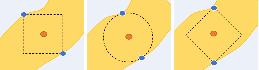
Figure 2: Critical $s$-balls with respect to Manhattan (left), Euclidean (middle) and Chebyshev (right) distance.

The essence of these examples is that the existence of multiple counterfactuals can cause robustness problems. In order to avoid the problem, we have to allow, at least, that counterfactual explainers return more than one counterfactual. However, even when returning multiple counterfactuals, $(\epsilon,k)$-robustness cannot be guaranteed because boundary counterfactuals (i.e., counterfactuals with distance $\operatorname{cfd}(\mathbf{x})+\epsilon$) are always lost when making an arbitrarily small step away from them. However, we can satisfy a weaker notion that guarantees that strong counterfactuals are preserved.

Definition 4 (Weak $\epsilon$-Robustness).

$E$ is weakly $\epsilon$-robust with respect to $d$ if for all inputs $\mathbf{x}_{1},\mathbf{x}_{2}\in\mathcal{D}$ such that $\operatorname{Cl}(\mathbf{x}_{1})=\operatorname{Cl}(\mathbf{x}_{2})$ and $d(\mathbf{x}_{1},\mathbf{x}_{2})<\epsilon$, we have that if $\mathbf{x}_{\mathbf{c}_{1}}\in E(\operatorname{Cl},\mathbf{x}_{1})$ is a strong counterfactual with respect to $\mathbf{x}_{1}$, then $\mathbf{x}_{\mathbf{c}_{1}}\in E(\operatorname{Cl},\mathbf{x}_{2})$

Conceptually, we can define a weakly $\frac{\epsilon}{2}$-robust counterfactual explainer by returning all $\epsilon$-approximate counterfactuals. We call the corresponding explainer the exhaustive $\epsilon$-approximate explainer and denote it by $E^{\epsilon}_{exh}$. Before showing that $E^{\epsilon}_{exh}$ is indeed $\frac{\epsilon}{2}$-robust, we state a simple lemma that is useful for proving robustness guarantees in general.

Lemma 2.

If $d$ satisfies the triangle inequality, then for all $\mathbf{x}_{1},\mathbf{x}_{2}\in\mathcal{D}$ such that $\operatorname{Cl}(\mathbf{x}_{1})=\operatorname{Cl}(\mathbf{x}_{2})$, we have $\operatorname{cfd}(\mathbf{x}_{1})\leq d(\mathbf{x}_{1},\mathbf{x}_{2})+\operatorname{cfd}(\mathbf{x}_{2})$.

Proof.

See Appendix. ∎

Proposition 1.

If $d$ satisfies Symmetry and the Triangle Inequality, then $E^{\epsilon}_{exh}$ is weakly $\frac{\epsilon}{2}$-robust.

Proof.

See Appendix. ∎

We give a geometrical illustration of the proposition in the appendix after the proof. The following example explains why we cannot give a general robustness guarantee for $\epsilon$-approximate counterfactuals that are not strong.

Example 2.

Consider again the example in Figure 1. Let $\epsilon>0$ be minimally chosen such that $\mathbf{c}$ is an $\epsilon$-approximate counterfactual for $\mathbf{x}_{2}$. Then, $\mathbf{c}\in E^{\epsilon}_{exh}(\operatorname{Cl},\mathbf{x}_{2})$. However, when we let $\mathbf{x}_{3}$ be another input on the line segment between $\mathbf{x}_{2}$ and $\mathbf{c}_{2}$, then we will lose $\mathbf{c}$ and all of its close neighbours in $E^{\epsilon}_{exh}(\operatorname{Cl},\mathbf{x}_{3})$.

Let us note, however, that this case only occurs in boundary cases. Intuitively, a counterfactual is safer the closer it is to a strong counterfactual. To make this intuition more precise, we define a notion of safety of counterfactuals based on a given input that is to be explained and the tolerance parameter $\epsilon$ of $E^{\epsilon}_{exh}$ (c.f., Def. 2).

Definition 5.

A counterfactual $\mathbf{c}$ of $\mathbf{x}$ is called $\delta$-safe with respect to $E^{\epsilon}_{exh}(\operatorname{Cl},\mathbf{x})$ if $\delta=\operatorname{cfd}(\mathbf{x})+\epsilon-d(\mathbf{x},\mathbf{c})$ and $\delta\geq 0$.

For example, strong counterfactuals are $\epsilon$-safe. Boundary $\epsilon$-approximate counterfactuals as in Example 2 are $0$-safe. All other $\epsilon$-approximate counterfactuals are $\delta$-safe for some $\delta\in(0,\epsilon)$. As we show next, $E^{\epsilon}_{exh}$ also gives us some robustness guarantees for $\delta$-safe counterfactuals that are not strong. Using our previous terminology, the following proposition roughly states that $E^{\epsilon}_{exh}$ is $\frac{\delta}{2}$-robust for $\delta$-safe counterfactuals.

Proposition 2.

Suppose that $d$ satisfies Symmetry and the Triangle Inequality. If $\mathbf{c}\in E^{\epsilon}_{exh}(\operatorname{Cl},\mathbf{x})$ is $\delta$-safe, then for all $\mathbf{x}^{\prime}\in\mathcal{D}$ such that $\operatorname{Cl}(\mathbf{x})=\operatorname{Cl}(\mathbf{x}^{\prime})$ and $d(\mathbf{x},\mathbf{x}^{\prime})<\frac{\delta}{2}$, we have $\mathbf{c}\in E^{\epsilon}_{exh}(\operatorname{Cl},\mathbf{x}^{\prime})$.

Proof.

See Appendix. ∎

Intuitively, $E^{\epsilon}_{exh}$ guarantees that the closer a counterfactual is to being a strong counterfactual, the further away we can move from the reference point without losing the counterfactual.

At this point, we know that $E^{\epsilon}_{exh}$ gives us some interesting robustness guarantees. However, $E^{\epsilon}_{exh}$ is not practical because the number of $\epsilon$-approximate counterfactuals is infinite in continuous domains and potentially exponentially large (with respect to the number of features) in discrete domains. In the next section, we will therefore focus on approximating $E^{\epsilon}_{exh}$ by a subset of diverse counterfactuals that provide a good tradeoff between explanation size and robustness guarantees.

5 Approximating $E^{\epsilon}_{exh}$

From a user perspective, there is no point in reporting a large set of counterfactuals that are all very similar. Instead, we should try to identify a small set of diverse counterfactuals that represent the counterfactuals in $E^{\epsilon}_{exh}$ well. We assume that our dataset $E$ is representative for the data that can occur in our domain and guide our search for representative counterfactuals by the examples that occur in $E$. Before describing our approach in more detail, we give a high-level overview of the four main steps it performs, which we also illustrate in Figure 3:

1. Order examples based on distance from input (Fig 3(a)).

2. Filter examples based on distance (Fig 3(b)).

3. Filter remaining examples based on diversity (Fig 3(c)).

4. For every remaining example, compute a corresponding counterfactual via binary search (Fig 3(d)).

(a)

(b)

(c)

(d)

Figure 3: Pictorial representation of steps 1-4 performed by our approach.

In step 1, we are given an input $\mathbf{x}$ with class $\operatorname{Cl}(\mathbf{x})=l$. We construct the set:

$$S_{1}=\{(\mathbf{x}^{\prime},d(\mathbf{x},\mathbf{x}^{\prime}))\mid(\mathbf{x}^{\prime},y)\in E,\operatorname{Cl}(\mathbf{x}^{\prime})\neq l\}$$ (7)

consisting of pairs of counterfactual points from $E$ and their distance to $\mathbf{x}$. We order the elements in $S_{1}$ according to the distance in increasing order.

In step 2, we restrict $S_{1}$ to the closest candidates. There are two natural options to cutoff candidates.

Number-based:

pick the $M$ closest candidates.

Distance-based:

pick all candidates within a tolerance threshold.

The number-based approach cannot adapt to different characteristics of $E$. For example, depending on whether the counterfactuals in $E$ are all very close (dense) or all very far away (sparse), we may want to make a different choice of $M$. The distance-based selection computes the minimum distance of a counterfactual in $E$:

$$m=\min_{(\mathbf{x}^{\prime},y^{\prime})\in E}d(\mathbf{x}^{\prime},\mathbf{x}),$$ (8)

and picks all candidates with distance at most $(1+\epsilon)\cdot m$ (all counterfactuals that are at most $100\cdot\epsilon\%$ more distant than the closest counterfactual). Hence, it will pick a larger number when $E$ is dense and a smaller number when $E$ is sparse. We let $S_{2}$ denote the set obtained from $S_{1}$ by picking the closest candidates according to our selection criterion:

$$S_{2}=distanceFilter(S_{1},\alpha),$$ (9)

where the parameter $\alpha$ determines the number of candidates (number-based) or the tolerance threshold $\epsilon$ (distance-based).

In step 3, we filter $S_{2}$ according to some diversity criterion. We consider two alternatives for this purpose.

Angle-based:

We quantify the difference between two counterfactuals $\mathbf{c}_{1},\mathbf{c}_{2}$ by the angle between them relative to the input $\mathbf{x}$. Formally, we compute the cosine distance between $(\mathbf{x}_{1}-\mathbf{x})$ and $(\mathbf{x}_{2}-\mathbf{x})$.

Distance-based:

Based on the distance between $\mathbf{c}_{1}$ and $\mathbf{c}_{2}$.

We create the filtered set $S_{3}$ in a greedy fashion. Starting with the set containing only the closest counterfactual, we successively add elements from $S_{2}$ (still ordered by distance) if they are sufficiently different from all candidates that have already been added. For the cosine distance, we use the intuition that the angle between the vectors should be sufficiently large. For the distance-based filter we demand that the distance between two counterfactuals is at least $100\cdot\beta\%$ more than $m$ (Equation 8) for some $\beta\in[0,1]$, which leads to the constraint $d(x,y)\geq(1+\beta)\cdot m$. We define $S_{3}$ by filtering $S_{2}$ based on the angle or distance.

$$S_{3}=diversityFilter(S_{2},\beta),$$ (10)

where the parameter $\beta$ determines the angular (angle-based) or distance (distance-based) threshold.

In step 4, we compute counterfactuals from the remaining candidates in $S_{3}$. To this end, we perform a binary search (Algorithm 1) for every $\mathbf{c}\in S_{3}$ to find the closest counterfactual to $\mathbf{x}$ on the line segment between $\mathbf{x}$ and $\mathbf{c}$. Our algorithm finally returns:

$$C=binarySearch(S_{3},\mathbf{x}).$$ (11)

Algorithm 1 Binary linear-search algorithm

1:reference point $\mathbf{x}$, counterfactual $\mathbf{c}$, desired accuracy $\gamma$

2:closest counterfactual on line segment between $\mathbf{x}$ and $\mathbf{c}$

3:while $d(\mathbf{x},\mathbf{c})>\gamma$ do

4:     $\mathbf{x}^{\prime}\leftarrow\frac{\mathbf{x}+\mathbf{c}}{2}$

5:     if $\operatorname{Cl}(\mathbf{x}^{\prime})=\operatorname{Cl}(\mathbf{x})$ then

6:         $\mathbf{x}\leftarrow\mathbf{x}^{\prime}$

7:     else

8:         $\mathbf{c}\leftarrow\mathbf{x}^{\prime}$      

9:return $\mathbf{c}$

We give a short runtime analysis of our algorithm in the following proposition.

Proposition 3.

Consider a classification problem with $k$ features and $N$ examples.

• Step 1 can be computed in time $O(N\cdot(k+\log N))$.

• Step 2 can be computed in time $O(N\cdot k)$.

• Let $M$ be the number of points remaining after step 2. Assuming that the distance can be computed in time $O(k)$, Step 3 can be computed in time $O(M^{2}\cdot k)$.

• Let $T_{\operatorname{Cl}}(k)$ be the runtime function of the classifier and let $D_{max}$ be the maximum distance between the reference point $\mathbf{x}$ and one of the remaining points. Step 4 can be computed in time $O(M\cdot(k+T_{\operatorname{Cl}}(k))\cdot\log_{2}\frac{D_{max}}{\gamma})$.

Proof.

See Appendix. ∎

Let us note that many classifiers can classify examples in linear time, that is, $T_{\operatorname{Cl}}(k)=O(k)$. The overall runtime is then roughly quadratic with respect to the number of features and the number of candidates remaining after step 2 and log-linear in the number of all examples.

We implemented a first prototype of our algorithm. Instead of sorting and maintaining the points manually, we use a k-d-tree. This is likely to increase runtime, but simplified the implementation.

6 Experimental Analysis

In the previous sections we laid the theoretical foundations for a framework to generate counterfactual explanations that are robust to changes in the input. We then introduced an approximation algorithm that uses diversity to generate robust counterfactual explanations while maintaining computational feasibility. In this section, we evaluate the performance of our approximation algorithm empirically. To this end, we compare our method with DiCE, the de-facto standard approach to generate sets of diverse counterfactual explanations. We study the robustness of the two methods along different metrics and show that our approach outperforms DiCE in most cases.

Experimental setup

Datasets. We consider five binary classification datasets commonly used in the literature: diabetes (Smith et al. 1988), no2 (Vanschoren et al. 2013), credit (Dua and Graff 2017), spambase (Hopkins et al. 1999) and online news popularity (Fernandes et al. 2015). Our selection includes both low- and high-dimensionality data, which allows to evaluate the applicability of our approach in both scenarios. We split each dataset into a training set and test set; more details about the datasets can be found in the appendix.

Models and algorithms. We train neural network classifier with two hidden layers ($20$ and $10$ neurons respectively) for each dataset and use two algorithms to generate diverse explanations: ours and DiCE (Mothilal, Sharma, and Tan 2020), which uses gradient-based optimisation to generate sets of explanations under a loss function that optimises their diversity and proximity to the input.

Hyperparameters. DiCE is run with default parameters from the respective library. As for our approach, the following configuration is used: number-based selection in Step 2 with $\alpha=50$ for diabetes and no2, and $\alpha=1000$ for the remaining datasets; angle-based filter with $\beta=0.5$ in Step 3 and $\gamma=0.1$ in Step 4. More details on hyperparameter selection can be found in the appendix.

Protocol. Counterfactual explanations are generated following the same protocol. Given an input $\mathbf{x}$ a set of counterfactual explanations is generated using one among the algorithms considered. Then, a Gaussian distribution centered at $\mathbf{x}$ is sampled to obtain a new input $\mathbf{x}_{2}$ of the same class. This input is then used to test the robustness of the counterfactual explainers as follows. The same counterfactual explanation algorithm is run on $\mathbf{x}_{2}$, the resulting set of counterfactual explanations is evaluated along different metrics that we describe in the next section. We run this protocol three times for each input $\mathbf{x}$ and collect average and standard deviation for each of the metrics we consider. We use this protocol to evaluate experimentally to which extent our approximation can maintain the theoretical robustness guarantees of $E^{\epsilon}_{exh}$.

Hardware. All experiments were conducted on standard PC running Ubuntu 20.04.6 LTS, with 15GB RAM and processor Intel(R) Core(TM) i7-8700 CPU @ 3.20GHz.

	diabetes				no2				news
	ours (L1)	DiCE (L1)	ours (L2)	DiCE (L2)	ours (L1)	DiCE (L1)	ours (L2)	DiCE (L2)	ours (L1)	DiCE (L1)	ours (L2)	DiCE (L2)
validity	100%	100%	100%	100%	100%	100%	100%	100%	100%	100%	100%	100%
$k$-distance	1.13 $\pm$ 0.43	1.83 $\pm$ 0.35	0.52 $\pm$ 0.20	1.06 $\pm$ 0.18	0.62 $\pm$0.23	1.26 $\pm$ 0.22	0.31 $\pm$ 0.11	0.80 $\pm$ 0.15	2.70 $\pm$ 0.97	3.59 $\pm$ 0.78	0.75 $\pm$ 0.27	1.47 $\pm$ 0.24
$k$-diversity	1.39 $\pm$ 0.46	1.32 $\pm$ 0.19	0.63 $\pm$ 0.22	0.77 $\pm$ 0.10	0.78 $\pm$ 0.28	0.87 $\pm$ 0.16	0.30 $\pm$ 0.14	0.50 $\pm$ 0.09	3.45 $\pm$ 1.24	1.91 $\pm$ 0.93	0.94 $\pm$ 0.35	0.78 $\pm$ 0.40
$\operatorname{set-distance}^{d}_{\Sigma}$	0.21 $\pm$ 0.20	0.33 $\pm$0.1	0.09 $\pm$ 0.03	0.18 $\pm$ 0.06	0.16 $\pm$ 0.12	0.87 $\pm$ 0.16	0.07 $\pm$ 0.05	0.16 $\pm$ 0.07	0.88 $\pm$ 0.78	1.73 $\pm$ 0.72	0.21 $\pm$ 0.21	0.61 $\pm$ 0.30
$\operatorname{set-distance}^{d}_{max}$	0.51 $\pm$ 0.44	0.66 $\pm$ 0.25	0.24 $\pm$ 0.20	0.38 $\pm$ 0.16	0.33 $\pm$ 0.24	0.47 $\pm$ 0.24	0.16 $\pm$ 0.11	0.26 $\pm$ 0.13	1.94 $\pm$ 1.41	2.59 $\pm$ 1.00	0.52 $\pm$ 0.44	0.94 $\pm$ 0.40
Time (s)	0.02 $\pm$ 0.00	72.66 $\pm$ 32.57	0.02 $\pm$ 0.00	75.22 $\pm$ 35.29	0.02 $\pm$ 0.01	130.78 $\pm$ 13.945	0.02 $\pm$ 0.01	129.13 $\pm$ 134. 66	0.30 $\pm$ 0.08	338.89 $\pm$ 11.59	0.30 $\pm$ 0.00	340.26 $\pm$ 117.52

Table 1: Comparison between DiCE and our method (angle-based) on $50$ instances for $\beta=0.5$ and $\gamma=0.1$ We report average and standard deviation for each metric (validity excluded).

	diabetes				no2				news
	ours (L1)	DiCE (L1)	ours (L2)	DiCE (L2)	ours (L1)	DiCE (L1)	ours (L2)	DiCE (L2)	ours (L1)	DiCE (L1)	ours (L2)	DiCE (L2)
validity	100%	100%	100%	100%	100%	100%	100%	100%	100%	100%	100%	100%
$k$-distance	1.38 $\pm$ 0.29	1.83 $\pm$ 0.35	0.64 $\pm$ 0.14	1.06 $\pm$ 0.18	0.87 $\pm$ 0.20	1.26 $\pm$ 0.22	0.43 $\pm$ 0.09	0.80 $\pm$ 0.15	3.53 $\pm$ 0.90	3.59 $\pm$ 0.78	0.98 $\pm$ 0.26	1.47 $\pm$ 0.24
$k$-diversity	1.71 $\pm$ 0.3	1.32 $\pm$ 0.19	0.78 $\pm$ 0.15	0.77 $\pm$ 0.10	1.11 $\pm$ 0.24	0.87 $\pm$ 0.16	0.55 $\pm$ 0.10	0.50 $\pm$ 0.09	4.35 $\pm$ 1.17	1.91 $\pm$ 0.93	1.20 $\pm$ 0.34	0.78 $\pm$ 0.40
$\operatorname{set-distance}^{d}_{\Sigma}$	0.22 $\pm$ 0.24	0.33 $\pm$0.1	0.10 $\pm$ 0.11	0.18 $\pm$ 0.06	0.15 $\pm$ 0.16	0.87 $\pm$ 0.16	0.07 $\pm$ 0.08	0.16 $\pm$ 0.07	0.79 $\pm$ 0.97	1.73 $\pm$ 0.72	0.21 $\pm$ 0.27	0.61 $\pm$ 0.30
$\operatorname{set-distance}^{d}_{max}$	0.63 $\pm$ 0.56	0.66 $\pm$ 0.25	0.29 $\pm$ 0.26	0.38 $\pm$ 0.16	0.39 $\pm$ 0.35	0.47 $\pm$ 0.24	0.18 $\pm$ 0.16	0.26 $\pm$ 0.13	2.14 $\pm$ 1.87	2.59 $\pm$ 1.00	0.61 $\pm$ 0.56	0.94 $\pm$ 0.40
Time (s)	0.01 $\pm$ 0.00	72.66 $\pm$ 32.57	0.01 $\pm$ 0.00	75.22 $\pm$ 35.29	0.01 $\pm$ 0.00	130.78 $\pm$ 13.945	0.01 $\pm$ 0.01	129.13 $\pm$ 134. 66	0.28 $\pm$ 0.01	338.89 $\pm$ 11.59	0.27 $\pm$ 0.04	340.26 $\pm$ 117.52

Table 2: Comparison between DiCE and our method (angle-based) on $50$ instances for $\beta=0.5$ and no minimisation. We report average and standard deviation for each metric (validity excluded).

Evaluation metrics

We evaluate results obtained using metrics that are specifically designed to assess the proximity and diversity of the explanations returned, as well as their robustness with respect to minor changes in the input to be explained. Formally, given a distance metric $dist:\mathcal{D}\times\mathcal{D}\rightarrow\mathbb{R}^{+}$, a factual input $\mathbf{x}$ and a set of diverse counterfactuals $S=\{\mathbf{x}^{\prime}_{1},\ldots,\mathbf{x}^{\prime}_{n}\}$, we consider:

• $k$-distance (Mohammadi et al. 2021), defined as:

  $$k\text{-distance}(\mathbf{x},S)=\frac{1}{\lvert S\rvert}\sum_{j=1}^{\lvert S\rvert}dist(\mathbf{x},\mathbf{x}^{\prime}_{j})$$ (12)

  to measure the distance of the diverse set of counterfactuals from the factual input. Low values imply lower cost of recourse.

• $k$-diversity (Mohammadi et al. 2021), defined as:

  $$k\text{-diversity}(S)=\frac{1}{{\lvert S\rvert\choose 2}}\sum_{j=1}^{\lvert S\rvert-1}\sum_{l=j+1}^{\lvert S\rvert}dist(\mathbf{x}^{\prime}_{j},\mathbf{x}^{\prime}_{l})$$ (13)

  to measure the distance between counterfactual explanations within the set $S$. Higher values indicate more diversity.

• in order to compare the robustness of generated counterfactuals, we use the average and maximum set distance as defined in equations (4) and (4)

In all our experiments we use the $L_{1}$ and $L_{2}$ distances to measure $dist$, as commonly done in the literature (Wachter, Mittelstadt, and Russell 2017; Mohammadi et al. 2021; Dutta et al. 2022; Jiang et al. 2023).

Evaluating robustness

This experiment is designed to show that our approach is able to generate diverse sets of explanations that are more robust than state-of-the-art algorithms. For each dataset, we select $20$ additional instances from the test set and generate sets of counterfactual explanations each following the protocol described earlier in this section. The number of diverse counterfactuals for each input is limited to a maximum of $5$ for each method so as to limit the cognitive load on the user. For better legibility, we only report results for three datasets; the full results can be found in the appendix.

Table 1 reports the results obtained for the overall best parameterisation $\beta=0.5$ and $\gamma=0.1$ under angle-based filtering. As we can observe, our approach consistently outperforms DiCE on several of the metrics considered across all the datasets. In particular, our explanations exhibit a higher degree of robustness compared to DiCE’s. Indeed, the distance between the two sets of counterfactuals generated by our algorithm for the original input and its perturbed version is always smaller than that of DiCE, demonstrating that our approach is successful at improving the robustness of the explanations it generates. As far as diversity is concerned, the results produced by the two appraoches are comparable for diabetes and no2. DiCE generates more diverse explanations for credit and spam, whereas our appraoch dominates in the news dataset. Overall we can observe that when DiCE achieves better diversity, it often sacrifices proximity; our approach instead always obtains better proximity, revealing a possible tension between the two metrics. Indeed, we hypothesise the diversity of our counterfactuals is affected by the minimisation of Step 4, which brings counterfactuals closer together thus leading to a decrease in $k$-diversity. Finally, we note that the time taken by DiCE to generate solutions is always significantly larger, reaching a two order of magnitude difference in the news dataset.

The effect of minimisation

To test the impact that minimisation may have on the diversity of counterfactuals generated by our method, we conducted another set of experiments where no minimisation is performed. We report the results obtained in Table 2, again using $\beta=0.5$ and angle-based filtering for better comparison. Overall, we observe that this configuration results in higher degrees of diversity when compared to the previous experiments. This appears to confirm our intuition that minimising distance reduces the diversity of the set returned. Removing minimisation results in higher $k$-distance from the original input; however, our approach still outperforms DiCE across all datasets. Overall, the robustness of our counterfactual explanations does not appear to be compromised as our approach always returns explanations that are more robust than DiCE’s; however we observe a slight increase in both robustness-related metrics, indicating a possible connection between $k$-diversity and robustness. Finally, we note that also in this case the runtime performance of our algorithm is superior to DiCE’s across all datasets considered.

7 Conclusions

In this paper we studied the robustness of counterfactual explanations with respect to minor changes in the input they were generated for. We discussed several limitations of current algorithms for generating counterfactual explanations and presented a novel framework to generate explanation with interesting robustness guarantees. While theoretically interesting, the number of counterfactuals that need to be reported can be infinite. Therefore, we introduced an approximation scheme that uses diversity to find a compact representation of the candidate counterfactuals and presented an empirical evaluation of the robustness of our approximation. Our results show that the resulting method improves the state-of-the-art in generating robust counterfactual explanations, while also showing great advantages in terms of computational performance. Future work will focus on devising tighter approximation schemes to further strengthen the robustness guarantees our framework can offer.

8 Proofs of Technical Results

Lemma 1.

• For all distance measures $d$, and all $\emptyset\subset S_{1},S_{2}\subseteq\mathcal{D}$, $\operatorname{set-distance}^{d}_{\sum}(S_{1},S_{2})\leq\operatorname{set-distance}^{d}_{\max}(S_{1},S_{2})$.

• If $d$ satisfies Symmetry, $S_{1}=\{\mathbf{c}_{1}\}$ and $S_{2}=\{\mathbf{c}_{2}\}$ ($S_{1}$ and $S_{2}$ contain a single point), then $\operatorname{set-distance}^{d}_{\sum}(S_{1},S_{2})=\operatorname{set-distance}^{d}_{\max}(S_{1},S_{2})=d(\mathbf{c}_{1},\mathbf{c}_{2})$.

Proof.

1. The claim follows from observing that $\frac{1}{\lvert S\rvert}\sum_{\mathbf{c}\in S}\min_{\mathbf{c}^{\prime}\in S^{\prime}}d(\mathbf{c},\mathbf{c}^{\prime})\leq\frac{\lvert S\rvert}{\lvert S\rvert}\max_{\mathbf{c}\in S}\min_{\mathbf{c}^{\prime}\in S^{\prime}}d(\mathbf{c},\mathbf{c}^{\prime})$ and the definitions.

2. Both measures evaluate to $\frac{1}{2}d(\mathbf{c}_{1},\mathbf{c}_{2})+\frac{1}{2}d(\mathbf{c}_{2},\mathbf{c}_{1})$, which is just $d(\mathbf{c}_{1},\mathbf{c}_{2})$ by Symmetry. ∎

Lemma 2.

If $d$ satisfies the triangle inequality, then for all $\mathbf{x}_{1},\mathbf{x}_{2}\in\mathcal{D}$ such that $\operatorname{Cl}(\mathbf{x}_{1})=\operatorname{Cl}(\mathbf{x}_{2})$, we have $\operatorname{cfd}(\mathbf{x}_{1})\leq d(\mathbf{x}_{1},\mathbf{x}_{2})+\operatorname{cfd}(\mathbf{x}_{2})$.

Proof.

First assume that there is a strong counterfactual $\mathbf{c}_{2}$ for $\mathbf{x}_{2}$. Since $\operatorname{Cl}(\mathbf{x}_{1})=\operatorname{Cl}(\mathbf{x}_{2})$, $\mathbf{c}_{2}$ is a (not necessarily strong) counterfactual for $\mathbf{x}_{1}$ as well and we have $\operatorname{cfd}(\mathbf{x}_{1})\leq d(\mathbf{x}_{1},\mathbf{c}_{2})\leq d(\mathbf{x}_{1},\mathbf{x}_{2})+d(\mathbf{x}_{2},\mathbf{c}_{2})=d(\mathbf{x}_{1},\mathbf{x}_{2})+\operatorname{cfd}(\mathbf{x}_{2})$.

If there is no strong counterfactual for $\mathbf{x}_{2}$, then, for every $\epsilon>0$, we can find a (non-strong) counterfactual $\mathbf{c}_{2}$ such that $d(\mathbf{x}_{2},\mathbf{x}_{2})<\operatorname{cfd}(\mathbf{x}_{2})+\epsilon$. As before, we can then conclude that $\operatorname{cfd}(\mathbf{x}_{1})\leq d(\mathbf{x}_{1},\mathbf{x}_{2})+\operatorname{cfd}(\mathbf{x}_{2})+\epsilon$. Since $\epsilon$ can be arbitrarily small, we can conclude that $\operatorname{cfd}(\mathbf{x}_{1})\leq d(\mathbf{x}_{1},\mathbf{x}_{2})+\operatorname{cfd}(\mathbf{x}_{2})$. ∎

Proposition 1.

If $d$ satisfies Symmetry and the Triangle Inequality, then $E^{\epsilon}_{exh}$ is weakly $\frac{\epsilon}{2}$-robust.

Proof.

Consider two inputs $\mathbf{x}_{1},\mathbf{x}_{2}\in\mathcal{D}$ such that $d(\mathbf{x}_{1},\mathbf{x}_{2})<\frac{\epsilon}{2}$. Assume that $\mathbf{c}_{1}\in E(\operatorname{Cl},\mathbf{x}_{1})$ is a strong counterfactual wrt. $\mathbf{x}_{1}$. Therefore, $d(\mathbf{x}_{2},\mathbf{c}_{1})\leq d(\mathbf{x}_{2},\mathbf{x}_{1})+d(\mathbf{x}_{1},\mathbf{c}_{1})<\frac{\epsilon}{2}+\operatorname{cfd}(\mathbf{x}_{1})\leq\frac{\epsilon}{2}+(\operatorname{cfd}(\mathbf{x}_{2})+\frac{\epsilon}{2})=\operatorname{cfd}(\mathbf{x}_{2})+\epsilon.$ Hence, $\mathbf{c}_{1}$ is an $\epsilon$-approximate counterfactual for $\mathbf{x}_{2}$ and therefore $\mathbf{x}_{\mathbf{c}_{1}}\in E^{\epsilon}_{exh}(\operatorname{Cl},\mathbf{x}_{2})$. ∎

We explain the geometrical intuition of the result in Figure 4.

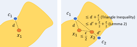
Figure 4: Illustration of the geometrical intuition of Proposition 1: As we move from $x_{1}$ to $x_{2}$ by less than $\frac{\epsilon}{2}$, the distance from the strong counterfactual $c_{1}$ for $x_{1}$ to $x_{2}$ cannot be larger than the counterfactual distance of $x_{1}$ plus $\frac{\epsilon}{2}$ by the triangle inequality. Furthermore, Lemma 2 guarantees that the difference between the counterfactual distances of $x_{1}$ and $x_{2}$ cannot be larger than $\frac{\epsilon}{2}$. Hence, the distance from $c_{1}$ to $x_{2}$ cannot be larger than $x_{2}$’s counterfactual distance plus $\epsilon$. $E^{\epsilon}_{exh}$ will therefore report it (see the proof of Proposition 1 for the algebraic argument).

Proposition 2.

Suppose that $d$ satisfies Symmetry and the Triangle Inequality. If $\mathbf{c}\in E^{\epsilon}_{exh}(\operatorname{Cl},\mathbf{x})$ is $\delta$-safe, then for all $\mathbf{x}^{\prime}\in\mathcal{D}$ such that $\operatorname{Cl}(\mathbf{x})=\operatorname{Cl}(\mathbf{x}^{\prime})$ and $d(\mathbf{x},\mathbf{x}^{\prime})<\frac{\delta}{2}$, we have $\mathbf{c}\in E^{\epsilon}_{exh}(\operatorname{Cl},\mathbf{x}^{\prime})$.

Proof.

We have $d(\mathbf{x}^{\prime},\mathbf{c})\leq d(\mathbf{x}^{\prime},\mathbf{x})+d(\mathbf{x},\mathbf{c})=\frac{\delta}{2}+(\operatorname{cfd}(\mathbf{x})+\epsilon-\delta)\leq\frac{\delta}{2}+(\operatorname{cfd}(\mathbf{x}^{\prime})+\frac{\delta}{2})+\epsilon-\delta=\operatorname{cfd}(\mathbf{x}^{\prime})+\epsilon$ and therefore $\mathbf{c}\in E^{\epsilon}_{exh}(\operatorname{Cl},\mathbf{x}^{\prime})$. ∎

Proposition 3.

Consider a classification problem with $k$ features and $N$ examples.

• Step 1 can be computed in time $O(N\cdot(k+\log N))$.

• Step 2 can be computed in time $O(N\cdot k)$.

• Let $M$ be the number of points remaining after step 2. Assuming that the distance can be computed in time $O(k)$, Step 3 can be computed in time $O(M^{2}\cdot k)$.

• Let $T_{\operatorname{Cl}}(k)$ be the runtime function of the classifier and let $D_{max}$ be the maximum distance between the reference point $\mathbf{x}$ and one of the remaining points. Step 4 can be computed in time $O(M\cdot(k+T_{\operatorname{Cl}}(k))\cdot\log_{2}\frac{D_{max}}{\gamma})$.

Proof.

1. Computing the distances from the examples to the reference point $\mathbf{x}$ has cost $O(N\cdot k)$. Ordering the points according to the distance with QuickSort has cost $O(N\cdot\log N)$.

2. Since the points have been ordered in step 1, we can just run through the array once, determine the cutoff point and copy the first points to a new array. The overall cost is $O(N\cdot k)$.

3. The first point can just be added to a new array. For the $i$-th point, $i>1$, we have to compute the distance/angle to the previously added points. Since at most $i-1$ points have been added at this point, the cost in the $i$-th iteration is $O((i-1)\cdot k)$ and the overall cost is $O(M^{2}\cdot k)$.

4. Let $D=d(\mathbf{x},\mathbf{c})$. Binary search updates $\mathbf{x}$ and $\mathbf{c}$ such that we halve the distance in every iteration. Hence, the distance after iteration $i$ is $\frac{D}{2^{i}}$. Hence, the termination criterion is reached after $\log_{2}\frac{D}{\gamma}$ iterations. Computing $\mathbf{x}^{\prime}$ and making the assignments can be done in time $O(k)$. Hence, the overall cost per iteration is $O(k+T_{\operatorname{Cl}}(k))$ an=d the overall cost of one binary search is $O((k+T_{\operatorname{Cl}}(k))\cdot\log_{2}\frac{D}{\gamma})$. Since we have to run the search for $M$ examples, the overall runtime is obtained from this bound by multiplying by $M$. ∎

9 Dataset details

Our experimental analysis uses five datasets for binary classification tasks, namely:

• the diabetes dataset, which is used to predict whether a patient has diabetes or not based on diagnostic measurements;

• the no2 dataset, which is used to predict whether nitrogen dioxide levels exceed a given threshold, based on measurements related to traffic volumes and metereological conditions;

• the credit dataset, which is used to predict the credit risk of a person (good or bad) based on a set of attribute describing their credit history;

• the spambase is used to predict whether an email is to be considered spam or not based on selected attributes of the email;

• the online news popularity dataset, referred to as news in the following, is used to predict the popularity of online articles.

Table 3 summarises the main features of the dataset used.

dataset	type	instances	variables
no2	numeric	500	7
diabetes	numeric	768	8
credit	numeric	2000	10
spambase	numeric	4600	57
online news	numeric	39644	58

Table 3: Dataset details.

Each dataset is split into a training set and a test set using the train_test_split method provided by the sklearn Python library, run with default parameters. Min max scaling is applied to all datasets to ease training.

10 Models

Training is performed using the PyTorch library. We use batch size of $8$ and $100$ epochs for each dataset and model. Table 4 reports the accuracy obtained for each dataset.

dataset	accuracy
no2	0.60
diabetes	0.70
credit	0.93
spambase	0.91
online news	0.65

Table 4: Model accuracy for each dataset.

11 Hyperparameter tuning

We performed hyperparameter tuning using $50$ counterfactual pairs not contained in our test set. We used $\beta\in\{0,0.1,0.2,0.3,0.4,0.5\}$ to assess the impact of our filtering criterion in Step 3 using both distance and angle-based filtering. Finally, we used $\gamma\in\{0.1,0.01,0.001\}$ to evaluate different precisions in Step 4. The overall best results were obtained using $\beta=0.5$ and $\gamma=0.1$, for which we report results in Tables 5, Table 6, Table 7 and Table 8. Results obtained for other parameter valuations can be found at the following url: https://github.com/fraleo/robust˙counterfactuals˙aaai24/tree/main/results. Angle-based filtering proved to yield the best overall results when compared to distance-based filtering; we therefore decided to use angle-based filtering for the experiments reported in the main body of the paper.

	diabetes				no2				credit				spambase				news
	ours (L1)	DiCE (L1)	ours (L2)	DiCE (L2)	ours (L1)	DiCE (L1)	ours (L2)	DiCE (L2)	ours (L1)	DiCE (L1)	ours (L2)	DiCE (L2)	ours (L1)	DiCE (L1)	ours (L2)	DiCE (L2)	ours (L1)	DiCE (L1)	ours (L2)	DiCE (L2)
validity	50/50	50/50	50/50	50/50	50/50	50/50	50/50	50/50	50/50	50/50	50/50	50/50	50/50	48/50	50/50	48/50	50/50	50/50	50/50	50/50
$k$-distance	1.22	1.90	0.55	1.09	0.78	1.28	0.37	0.83	0.78	1.91	0.39	1.18	0.74	7.83	0.26	1.94	2.60	4.18	0.75	1.66
$k$-diversity	1.39	1.29	0.63	0.75	0.96	0.91	0.45	0.54	0.96	2.02	0.46	1.09	0.45	8.62	0.15	2.00	3.36	2.04	0.94	0.84
$\operatorname{set-distance}^{d}_{\Sigma}$	0.25	0.33	0.11	0.18	0.19	0.27	0.09	0.16	0.35	0.78	0.18	0.42	0.59	3.73	0.15	0.93	0.71	1.89	0.18	0.67
$\operatorname{set-distance}^{d}_{max}$	0.59	0.64	0.26	0.36	0.41	0.47	0.19	0.28	0.71	1.35	0.35	0.73	0.73	7.12	0.20	1.69	1.82	2.90	0.49	1.06
Time (s)	0.02	69.66	0.02	69.19	0.02	138.66	0.02	140.18	0.22	374.92	0.22	381.57	0.15	188.95	0.14	176.75	0.29	351.52	0.30	320.53

Table 5: Comparison between our method (angle-based) and DiCE on $50$ instances for $\beta=0.5$ and $\gamma=0.1$.

	diabetes				no2				credit				spambase				news
	ours (L1)	DiCE (L1)	ours (L2)	DiCE (L2)	ours (L1)	DiCE (L1)	ours (L2)	DiCE (L2)	ours (L1)	DiCE (L1)	ours (L2)	DiCE (L2)	ours (L1)	DiCE (L1)	ours (L2)	DiCE (L2)	ours (L1)	DiCE (L1)	ours (L2)	DiCE (L2)
validity	50/50	50/50	50/50	50/50	50/50	50/50	50/50	50/50	50/50	50/50	50/50	50/50	50/50	48/50	50/50	48/50	50/50	50/50	50/50	50/50
$k$-distance	1.13	1.90	0.57	1.09	0.71	1.28	0.38	0.83	0.63	1.91	0.42	1.18	0.74	7.83	0.26	1.94	2.32	4.18	0.82	1.66
$k$-diversity	0.93	1.29	0.63	0.75	0.71	0.91	0.47	0.54	0.53	2.02	0.50	1.09	0.55	8.62	0.13	2.00	2.48	2.04	1.03	0.84
$\operatorname{set-distance}^{d}_{\Sigma}$	0.12	0.33	0.13	0.18	0.13	0.27	0.11	0.16	0.10	0.78	0.22	0.42	0.36	3.73	0.17	0.93	0.42	1.89	0.63	0.67
$\operatorname{set-distance}^{d}_{max}$	0.44	0.64	0.26	0.36	0.35	0.47	0.23	0.28	0.33	1.35	0.37	0.73	0.65	7.12	0.21	1.69	0.93	2.90	0.23	1.06
Time (s)	0.03	69.66	0.02	69.19	0.02	138.66	0.02	140.18	0.19	374.92	0.16	381.57	0.10	188.95	0.07	176.75	0.28	351.52	0.24	320.53

Table 6: Comparison between our method (distance-based) and DiCE on $50$ instances for $\beta=0.5$ and $\gamma=0.1$.

	diabetes				no2				credit				spambase				news
	ours (L1)	DiCE (L1)	ours (L2)	DiCE (L2)	ours (L1)	DiCE (L1)	ours (L2)	DiCE (L2)	ours (L1)	DiCE (L1)	ours (L2)	DiCE (L2)	ours (L1)	DiCE (L1)	ours (L2)	DiCE (L2)	ours (L1)	DiCE (L1)	ours (L2)	DiCE (L2)
validity	50/50	50/50	50/50	50/50	50/50	50/50	50/50	50/50	50/50	50/50	50/50	50/50	50/50	48/50	50/50	48/50	50/50	50/50	50/50	50/50
$k$-distance	1.45	1.90	0.66	1.09	0.97	1.28	0.46	0.83	0.82	1.91	0.41	1.18	0.97	7.83	0.34	1.94	3.42	4.18	0.99	1.66
$k$-diversity	1.69	1.29	0.77	0.75	1.18	0.91	0.55	0.54	1.00	2.02	0.45	1.09	0.65	8.62	0.23	2.00	4.32	2.04	1.23	0.84
$\operatorname{set-distance}^{d}_{\Sigma}$	0.27	0.33	0.12	0.18	0.18	0.27	0.09	0.16	0.36	0.78	0.18	0.42	0.50	3.73	0.17	0.93	0.58	1.89	0.17	0.67
$\operatorname{set-distance}^{d}_{max}$	0.69	0.64	0.32	0.36	0.46	0.47	0.23	0.28	0.73	1.35	0.37	0.73	0.76	7.12	0.25	1.69	2.05	2.90	0.60	1.06
Time (s)	0.01	69.66	0.01	69.19	0.01	138.66	0.05	140.18	0.20	374.92	0.20	381.57	0.14	188.95	0.14	176.75	0.28	351.52	0.28	320.53

Table 7: Comparison between our method (angle-based) and DiCE on $50$ instances for $\beta=0.5$ and no minimisation.

	diabetes				no2				credit				spambase				news
	ours (L1)	DiCE (L1)	ours (L2)	DiCE (L2)	ours (L1)	DiCE (L1)	ours (L2)	DiCE (L2)	ours (L1)	DiCE (L1)	ours (L2)	DiCE (L2)	ours (L1)	DiCE (L1)	ours (L2)	DiCE (L2)	ours (L1)	DiCE (L1)	ours (L2)	DiCE (L2)
validity	50/50	50/50	50/50	50/50	50/50	50/50	50/50	50/50	50/50	50/50	50/50	50/50	50/50	48/50	50/50	48/50	50/50	50/50	50/50	50/50
$k$-distance	1.30	1.90	0.72	1.09	0.90	1.28	0.49	0.83	0.67	1.91	0.45	1.18	0.92	7.83	0.35	1.94	3.05	4.18	1.08	1.66
$k$-diversity	1.08	1.29	0.82	0.75	0.87	0.91	0.57	0.54	0.56	2.02	0.52	1.09	0.66	8.62	0.21	2.00	3.15	2.04	1.35	0.84
$\operatorname{set-distance}^{d}_{\Sigma}$	0.10	0.33	0.15	0.18	0.11	0.27	0.12	0.16	0.09	0.78	0.25	0.42	0.21	3.73	0.20	0.93	0.17	1.89	0.29	0.67
$\operatorname{set-distance}^{d}_{max}$	0.45	0.64	0.32	0.36	0.41	0.47	0.27	0.28	0.33	1.35	0.39	0.73	0.59	7.12	0.26	1.69	0.74	2.90	0.83	1.06
Time (s)	0.01	69.66	0.01	69.19	0.01	138.66	0.01	140.18	0.18	374.92	0.15	381.57	0.09	188.95	0.07	176.75	0.25	351.52	0.24	320.53

Table 8: Comparison between our method (distance-based) and DiCE on $50$ instances for $\beta=0.5$ and no minimisation.

12 Full results Section 6

Tables 9 and 10 report the full results obtained for the five datasets considered in Section 6.

	diabetes				no2				credit				spambase				news
	ours (L1)	DiCE (L1)	ours (L2)	DiCE (L2)	ours (L1)	DiCE (L1)	ours (L2)	DiCE (L2)	ours (L1)	DiCE (L1)	ours (L2)	DiCE (L2)	ours (L1)	DiCE (L1)	ours (L2)	DiCE (L2)	ours (L1)	DiCE (L1)	ours (L2)	DiCE (L2)
validity	100%	100%	100%	100%	100%	100%	100%	100%	100%	100%	100%	100%	100%	89&	100%	89%	100%	100%	100%	100%
$k$-distance	1.13 $\pm$ 0.43	1.83 $\pm$ 0.35	0.52 $\pm$ 0.20	1.06 $\pm$ 0.18	0.62 $\pm$0.23	1.26 $\pm$ 0.22	0.31 $\pm$ 0.11	0.80 $\pm$ 0.15	0.85 $\pm$ 0.33	1.87 $\pm$0.34	0.41 $\pm$ 0.15	1.17 $\pm$ 0.18	1.12 $\pm$ 1.27	7.26 $\pm$ 2.73	0.38 $\pm$0.39	1.87 $\pm$ 0.57	2.70 $\pm$ 0.97	3.59 $\pm$ 0.78	0.75 $\pm$ 0.27	1.47 $\pm$ 0.24
$k$-diversity	1.39 $\pm$ 0.46	1.32 $\pm$ 0.19	0.63 $\pm$ 0.22	0.77 $\pm$ 0.10	0.78 $\pm$ 0.28	0.87 $\pm$ 0.16	0.30 $\pm$ 0.14	0.50 $\pm$ 0.09	1.02 $\pm$ 0.37	1.98 $\pm$ 0.31	0.48 $\pm$ 0.16	1.08 $\pm$ 0.16	0.61 $\pm$ 0.50	8.02 $\pm$ 2.77	0.20 $\pm$ 0.16	1.92 $\pm$ 0.55	3.45 $\pm$ 1.24	1.91 $\pm$ 0.93	0.94 $\pm$ 0.35	0.78 $\pm$ 0.40
$\operatorname{set-distance}^{d}_{\Sigma}$	0.21 $\pm$ 0.20	0.33 $\pm$0.1	0.09 $\pm$ 0.03	0.18 $\pm$ 0.06	0.16 $\pm$ 0.12	0.87 $\pm$ 0.16	0.07 $\pm$ 0.05	0.16 $\pm$ 0.07	0.35 $\pm$ 0.18	0.72 $\pm$ 0.21	0.17 $\pm$ 0.08	0.39 $\pm$ 0.11	0.50 $\pm$ 0.23	4.20 $\pm$ 1.52	0.14 $\pm$0.08	1.05 $\pm$ 0.37	0.88 $\pm$ 0.78	1.73 $\pm$ 0.72	0.21 $\pm$ 0.21	0.61 $\pm$ 0.30
$\operatorname{set-distance}^{d}_{max}$	0.51 $\pm$ 0.44	0.66 $\pm$ 0.25	0.24 $\pm$ 0.20	0.38 $\pm$ 0.16	0.33 $\pm$ 0.24	0.47 $\pm$ 0.24	0.16 $\pm$ 0.11	0.26 $\pm$ 0.13	0.76 $\pm$ 0.32	1.24 $\pm$ 0.31	0.37 $\pm$ 0.15	0.67 $\pm$0.18	0.73 $\pm$ 0.38	7.32 $\pm$ 2.37	0.21 $\pm$ 0.12	1.75 $\pm$ 0.49	1.94 $\pm$ 1.41	2.59 $\pm$ 1.00	0.52 $\pm$ 0.44	0.94 $\pm$ 0.40
Time (s)	0.02 $\pm$ 0.00	72.66 $\pm$ 32.57	0.02 $\pm$ 0.00	75.22 $\pm$ 35.29	0.02 $\pm$ 0.01	130.78 $\pm$ 13.945	0.02 $\pm$ 0.01	129.13 $\pm$ 134. 66	0.22 $\pm$ 0.02	396.71 $\pm$ 3.72	0.22 $\pm$ 0.02	413.09 $\pm$ 23.15	0.15 $\pm$ 0.01	203.19 $\pm$ 125.03	0.14 $\pm$ 0.01	205.58 $\pm$ 126.87	0.30 $\pm$ 0.08	338.89 $\pm$ 11.59	0.30 $\pm$ 0.00	340.26 $\pm$ 117.52

Table 9: Comparison between our method (angle-based) and DiCE on $50$ instances for $\beta=0.5$ and $\gamma=0.1$ We report average and standard deviation for each metric (validity excluded).

	diabetes				no2				credit				spambase				news
	ours (L1)	DiCE (L1)	ours (L2)	DiCE (L2)	ours (L1)	DiCE (L1)	ours (L2)	DiCE (L2)	ours (L1)	DiCE (L1)	ours (L2)	DiCE (L2)	ours (L1)	DiCE (L1)	ours (L2)	DiCE (L2)	ours (L1)	DiCE (L1)	ours (L2)	DiCE (L2)
validity	100%	100%	100%	100%	100%	100%	100%	100%	100%	100%	100%	100%	100%	89&	100%	89%	100%	100%	100%	100%
$k$-distance	1.38 $\pm$ 0.29	1.83 $\pm$ 0.35	0.64 $\pm$ 0.14	1.06 $\pm$ 0.18	0.87 $\pm$ 0.20	1.26 $\pm$ 0.22	0.43 $\pm$ 0.09	0.80 $\pm$ 0.15	0.88 $\pm$ 0.33	1.87 $\pm$0.34	0.42 $\pm$ 0.15	1.17 $\pm$ 0.18	1.29 $\pm$ 1.23	7.26 $\pm$ 2.73	0.46 $\pm$0.38	1.87 $\pm$ 0.57	3.53 $\pm$ 0.90	3.59 $\pm$ 0.78	0.98 $\pm$ 0.26	1.47 $\pm$ 0.24
$k$-diversity	1.71 $\pm$ 0.3	1.32 $\pm$ 0.19	0.78 $\pm$ 0.15	0.77 $\pm$ 0.10	1.11 $\pm$ 0.24	0.87 $\pm$ 0.16	0.55 $\pm$ 0.10	0.50 $\pm$ 0.09	1.06 $\pm$ 0.36	1.98 $\pm$ 0.31	0.51 $\pm$ 0.56	1.08 $\pm$ 0.16	0.74 $\pm$ 0.54	8.02 $\pm$ 2.77	0.26 $\pm$ 0.19	1.92 $\pm$ 0.55	4.35 $\pm$ 1.17	1.91 $\pm$ 0.93	1.20 $\pm$ 0.34	0.78 $\pm$ 0.40
$\operatorname{set-distance}^{d}_{\Sigma}$	0.22 $\pm$ 0.24	0.33 $\pm$0.1	0.10 $\pm$ 0.11	0.18 $\pm$ 0.06	0.15 $\pm$ 0.16	0.87 $\pm$ 0.16	0.07 $\pm$ 0.08	0.16 $\pm$ 0.07	0.35 $\pm$ 0.18	0.72 $\pm$ 0.21	0.18 $\pm$ 0.08	0.39 $\pm$ 0.11	0.45 $\pm$ 0.32	4.20 $\pm$ 1.52	0.16 $\pm$ 0.10	1.05 $\pm$ 0.37	0.79 $\pm$ 0.97	1.73 $\pm$ 0.72	0.21 $\pm$ 0.27	0.61 $\pm$ 0.30
$\operatorname{set-distance}^{d}_{max}$	0.63 $\pm$ 0.56	0.66 $\pm$ 0.25	0.29 $\pm$ 0.26	0.38 $\pm$ 0.16	0.39 $\pm$ 0.35	0.47 $\pm$ 0.24	0.18 $\pm$ 0.16	0.26 $\pm$ 0.13	0.78 $\pm$ 0.33	1.24 $\pm$ 0.31	0.39 $\pm$ 0.15	0.67 $\pm$0.18	0.76 $\pm$ 0.43	7.32 $\pm$ 2.37	0.26 $\pm$ 0.15	1.75 $\pm$ 0.49	2.14 $\pm$ 1.87	2.59 $\pm$ 1.00	0.61 $\pm$ 0.56	0.94 $\pm$ 0.40
Time (s)	0.01 $\pm$ 0.00	72.66 $\pm$ 32.57	0.01 $\pm$ 0.00	75.22 $\pm$ 35.29	0.01 $\pm$ 0.00	130.78 $\pm$ 13.945	0.01 $\pm$ 0.01	129.13 $\pm$ 134. 66	0.21 $\pm$ 0.03	396.71 $\pm$ 3.72	0.21 $\pm$ 0.01	413.09 $\pm$ 23.15	0.14 $\pm$ 0.01	203.19 $\pm$ 125.03	0.14 $\pm$ 0.01	205.58 $\pm$ 126.87	0.28 $\pm$ 0.01	338.89 $\pm$ 11.59	0.27 $\pm$ 0.04	340.26 $\pm$ 117.52

Table 10: Comparison between our method (angle-based) and DiCE on $50$ instances for $\beta=0.5$ and no minimisation. We report average and standard deviation for each metric (validity excluded).

References

- Black, Wang, and Fredrikson (2022) Black, E.; Wang, Z.; and Fredrikson, M. 2022. Consistent Counterfactuals for Deep Models. In Proceedings of the International Conference on Learning Representations (ICLR’22). OpenReview.net.
- Dua and Graff (2017) Dua, D.; and Graff, C. 2017. UCI Machine Learning Repository. http://archive.ics.uci.edu/ml. Accessed: 2022-08-30.
- Dutta et al. (2022) Dutta, S.; Long, J.; Mishra, S.; Tilli, C.; and Magazzeni, D. 2022. Robust Counterfactual Explanations for Tree-Based Ensembles. In Proceedings of the International Conference on Machine Learning (ICML’22), volume 162, 5742–5756. PMLR.
- Fernandes et al. (2015) Fernandes, K.; Vinagre, P.; Cortez, P.; and Sernadela, P. 2015. Online News Popularity. UCI Machine Learning Repository. DOI: https://doi.org/10.24432/C5NS3V.
- FICO Community (2019) FICO Community. 2019. Explainable Machine Learning Challenge. https://community.fico.com/s/explainable-machine-learning-challenge.
- Fokkema, de Heide, and van Erven (2022) Fokkema, H.; de Heide, R.; and van Erven, T. 2022. Attribution-based Explanations that Provide Recourse Cannot be Robust. arXiv preprint arXiv:2205.15834.
- Guidotti et al. (2019) Guidotti, R.; Monreale, A.; Ruggieri, S.; Turini, F.; Giannotti, F.; and Pedreschi, D. 2019. A Survey of Methods for Explaining Black Box Models. ACM Comput. Surv., 51(5): 93:1–93:42.
- Hancox-Li (2020) Hancox-Li, L. 2020. Robustness in machine learning explanations: does it matter? In Proceedings of the ACM Conference on Fairness, Accountability, and Transparency (FAT*’20), 640–647. ACM.
- Hopkins et al. (1999) Hopkins, M.; Reeber, E.; Forman, G.; and Suermondt, J. 1999. Spambase. UCI Machine Learning Repository. DOI: https://doi.org/10.24432/C53G6X.
- Jiang et al. (2023) Jiang, J.; Leofante, F.; Rago, A.; and Toni, F. 2023. Formalising the Robustness of Counterfactual Explanations for Neural Networks. In Procedings of the 37th AAAI Conference on Artificial Intelligence (AAAI’23), 14901–14909. AAAI Press.
- Karimi et al. (2020) Karimi, A.; Barthe, G.; Balle, B.; and Valera, I. 2020. Model-Agnostic Counterfactual Explanations for Consequential Decisions. In Proceedings of the 23rd International Conference on Artificial Intelligence and Statistics (AISTATS’20), 895–905.
- Karimi et al. (2023) Karimi, A.; Barthe, G.; Schölkopf, B.; and Valera, I. 2023. A Survey of Algorithmic Recourse: Contrastive Explanations and Consequential Recommendations. ACM Comput. Surv., 55(5): 95:1–95:29.
- Leofante, Botoeva, and Rajani (2023) Leofante, F.; Botoeva, E.; and Rajani, V. 2023. Counterfactual Explanations and Model Multiplicity: a Relational Verification View. In Proceedings of the 20th International Conference on Principles of Knowledge Representation and Reasoning (KR’23), 763–768.
- Leofante and Lomuscio (2023) Leofante, F.; and Lomuscio, A. 2023. Towards Robust Contrastive Explanations for Human-Neural Multi-Agent Systems. In Proceedings of the 22nd International Conference on Autonomous Agents and Multiagent Systems (AAMAS’23), 2343–2345.
- Mohammadi et al. (2021) Mohammadi, K.; Karimi, A.; Barthe, G.; and Valera, I. 2021. Scaling Guarantees for Nearest Counterfactual Explanations. In Proceedings of the AAAI/ACM Conference on AI, Ethics, and Society (AIES’21 )., 177–187. ACM.
- Mothilal, Sharma, and Tan (2020) Mothilal, R. K.; Sharma, A.; and Tan, C. 2020. Explaining machine learning classifiers through diverse counterfactual explanations. In Proceedings of the ACM Conference on Fairness, Accountability, and Transparency (FAT*’20)., 607–617.
- Pawelczyk, Broelemann, and Kasneci (2020) Pawelczyk, M.; Broelemann, K.; and Kasneci, G. 2020. On Counterfactual Explanations under Predictive Multiplicity. In Proceedings of the 36th Conference on Uncertainty in Artificial Intelligence (UAI’20), volume 124 of Proceedings of Machine Learning Research, 809–818. AUAI Press.
- Pawelczyk et al. (2023) Pawelczyk, M.; Datta, T.; van den Heuvel, J.; Kasneci, G.; and Lakkaraju, H. 2023. Probabilistically Robust Recourse: Navigating the Trade-offs between Costs and Robustness in Algorithmic Recourse. In Proceedings of the 11th International Conference on Learning Representations, (ICLR’23). OpenReview.net.
- ProPublica (2016) ProPublica. 2016. How We Analyzed the COMPAS Recidivism Algorithm . https://www.propublica.org/article/how-we-analyzed-the-compas-recidivism-algorithm.
- Slack et al. (2021) Slack, D.; Hilgard, A.; Lakkaraju, H.; and Singh, S. 2021. Counterfactual Explanations Can Be Manipulated. In Advances in Neural Information Processing Systems 34 (NeurIPS’21), 62–75.
- Smith et al. (1988) Smith, J. W.; Everhart, J. E.; Dickson, W.; Knowler, W. C.; and Johannes, R. S. 1988. Using the ADAP learning algorithm to forecast the onset of diabetes mellitus. In Proceedings of the annual symposium on computer application in medical care, 261. American Medical Informatics Association.
- Stepin et al. (2021) Stepin, I.; Alonso, J. M.; Catalá, A.; and Pereira-Fariña, M. 2021. A Survey of Contrastive and Counterfactual Explanation Generation Methods for Explainable Artificial Intelligence. IEEE Access, 9: 11974–12001.
- Upadhyay, Joshi, and Lakkaraju (2021) Upadhyay, S.; Joshi, S.; and Lakkaraju, H. 2021. Towards Robust and Reliable Algorithmic Recourse. In Advances in Neural Information Processing Systems 34 (NeurIPS’21), 16926–16937.
- Van Looveren and Klaise (2021) Van Looveren, A.; and Klaise, J. 2021. Interpretable Counterfactual Explanations Guided by Prototypes. In Proceedings of the European Conference on Machine Learning and Knowledge Discovery in Databases (ECML PKDD’21), 650–665.
- Vanschoren et al. (2013) Vanschoren, J.; van Rijn, J. N.; Bischl, B.; and Torgo, L. 2013. OpenML: networked science in machine learning. SIGKDD Explor., 15(2): 49–60.
- Wachter, Mittelstadt, and Russell (2017) Wachter, S.; Mittelstadt, B. D.; and Russell, C. 2017. Counterfactual Explanations without Opening the Black Box: Automated Decisions and the GDPR. Harv. JL & Tech., 31: 841.