TaCo: Targeted Concept Removal in Output Embeddings for NLP via Information Theory and Explainability

Abstract

The fairness of Natural Language Processing (NLP) models has emerged as a crucial concern. Information theory indicates that to achieve fairness, a model should not be able to predict sensitive variables, such as gender, ethnicity, and age. However, information related to these variables often appears implicitly in language, posing a challenge in identifying and mitigating biases effectively.
To tackle this issue, we present a novel approach that operates at the embedding level of an NLP model, independent of the specific architecture. Our method leverages insights from recent advances in XAI techniques and employs an embedding transformation to eliminate implicit information from a selected variable. By directly manipulating the embeddings in the final layer, our approach enables a seamless integration into existing models without requiring significant modifications or retraining.
In evaluation, we show that the proposed post-hoc approach significantly reduces gender-related associations in NLP models while preserving the overall performance and functionality of the models.
An implementation of our method is available: https://github.com/fanny-jourdan/TaCo

1 Introduction

The multiple and impressive successes of Artificial Intelligence and Machine Learning have made them more and more ubiquitous in applications where a model’s decisions has genuine repercussions on people’s lives. These decisions, however, typically come with biases that can lead to unfair, unethical consequences. To guard against such consequences, we must identify and understand the biased information these models utilize. This links the task of ensuring an ethical comportment of a model with its interpretability or explainability: if we can show the real reasons or features why a model makes the predictions or recommendations it does, then we can control for biases among these features.

In this paper, we propose a method for finding factors that influence model predictions using an algebraic decomposition of the latent representations of the model into orthogonal dimensions. Using the method of Singular Value Decomposition (SVD), which is well suited to our particular test case, we isolate various dimensions that contribute to a prediction. As our case study, we study the use of gender information in predicting occupations in the Bios dataset De-Arteaga et al. (2019) by a RoBERTa model Liu et al. (2019a). By intervening on the latent representations to remove certain dimensions and running the model on the edited representations, we show first a causal connection between various dimensions and model predictions about gender and separately about occupation. This enables us then to eliminate dimensions in the decomposition that convey gender bias in the decision without much affecting the model’s predictive performance on occupations. Because SVD gives us orthogonal dimensions, we know that once we have removed a dimension, the information it contains is no longer in the model.

Crucially, we show how to link various dimensions in the SVD decomposition of the latent representation with concepts like gender and its linguistic manifestations that matter to fairness, providing not only a faithful explanation of the model’s behaviour but a humanly understandable or plausible one as well. Faithfulness provides a causal connection and produces factors necessary and sufficient for the model to produce its prediction given a certain input. Plausibility has to do with how acceptable the purported explanation is to humans Jacovi and Goldberg (2020).

In addition, we demonstrate that our method can reach close to the theoretically ideal point of minimizing algorithmic bias while preserving strong predictive accuracy, and we offer a way of quantifying various operations on representations. Our method also has a relatively low computational cost, as we detail below. In principle, our approach applies to any type of deep learning model; it also can apply to representations that are generated at several levels, as in modern transformer architectures with multiple attention layers Vaswani et al. (2017). As such it can serve as a diagnostic tool for exploring complex deep learning models.

2 Related work

2.1 Gender Bias in Natural Language Processing models

In this paper, we aim to enhance the fairness of our model by employing a prevalent approach in information theory, which involves eliminating gender-related information to prevent the model from utilizing it Kilbertus et al. (2017), which is not the only way of obtaining gender-unbiased models.

A first approach in the literature is to remove explicit gender indicators (he, she, her, etc.) directly from the dataset De-Arteaga et al. (2019). However, modern transformer models have been shown to be able to learn implicit gender indicators Devlin et al. (2018); Karita et al. (2019). This essentially limits the impact that such a naive approach can have on this kind of models. As a matter of fact, a RoBERTa model trained without these gender indicators can still predict with upwards of 90% accuracy the gender of a person writing a short LinkedIn bio (see Appendix A).

Another approach attempts to create word embeddings that do not exhibit gender bias Bolukbasi et al. (2016); Garg et al. (2018); Zhao et al. (2018a, b); Caliskan et al. (2017); Bolukbasi et al. (2016); Zhao et al. (2019). Although interesting in principle, Gonen and Goldberg (2019) shows these methods may camouflage gender biases in word embeddings, but fail to eliminate them entirely.

A third approach, and more in line with our proposed method, consists in intervening in the model’s latent space. In Liang et al. (2020), the authors introduce a technique based on decomposing the latent space using a PCA and subtracting from the inputs the projection into a bias subspace that carries the most information about the target concept. Another vein focuses on modifying the latent space with considerations coming from the field of information theory Xu et al. (2020). Indeed, the $\nu$-information – a generalization of the mutual information – has been used as a means to carefully remove from the model’s latent space only the information related to the target concept. In particular, popular approaches include the removal of information through linear adversarials on the last layer of the model Ravfogel et al. (2020, 2022), through Assignment-Maximization adversarials Shao et al. (2023), and through linear models that act on the whole model Belrose et al. (2023). However, Ravfogel et al. (2023) recently discovered a limitation of guarding with log-linear models on multi-class tasks and warn about the choice of the model used for guarding against the target concept – e.g. gender. Fortunately, due to the way we choose to remove information, our method will not be affected by it.

Specifically, we propose to use methodology from the field of explainable AI (XAI) to perform feature selection to reduce the effect of algorithmic bias Frye et al. (2020); Dorleon et al. (2022); Galhotra et al. (2022) in a human-understandable yet principled manner. Indeed, our aim is to decompose the model’s embedding into an interpretable base of concepts – i.e. our features –, select those that carry the most information about gender and the least about the actual task, and suppress them from the embedding. We would thus be guarding against gender without a specific parametric model, and thus, less surgically precise, but more interpretable in our interventions than the literature: a trade-off than can be enticing in certain applications.

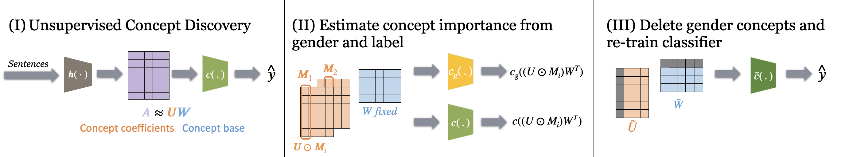
Figure 1: Overview of our method. The SVD decomposition (I) yields concepts, whose importance (II) with respect to gender and occupation are evaluated with Sobol method. Finally, some concepts are removed, which “neutralizes” the gender information and (III) produces a fairer classifier.

2.2 Explainability and Interpretability in Model Analysis

Explainability

Explanainable AI (XAI) is a domain that aims to expand the understanding of ML models and their inner workings, and to explain their predictions. We will take inspiration from this field to create a technique that allow us to debias models, and to do so in an interpretable manner.

Classical approaches analyze how each part of the input influences the model’s prediction, either through perturbation Ribeiro et al. (2016); Zeiler and Fergus (2014); Petsiuk et al. (2018) or by leveraging the gradients inside the neural network Sundararajan et al. (2017); Smilkov et al. (2017). However, these methods are prone to adversarial manipulation Wang et al. (2020), perform only partial input recovery Adebayo et al. (2018), and exhibit a general lack of stability with respect to the input Ghorbani et al. (2019). Moreover, they often fail to provide full interpretability because they provide explanations that tamper with some features but not others; in general the features tampered with do not offer a guarantee of the outcome Ignatiev et al. (2019); Marques-Silva (2023).

In NLP, the field of rationalization also play a pivotal role in enhancing our understanding by decomposing the prediction process into two: one model proposes excerpts from the input and another predicts based on them, thus allowing users to identify the parts of the input that are being used to predict the answer Lei et al. (2016); Bastings et al. (2019); Jain et al. (2020); Antognini and Faltings (2021).

Other approaches include counterfactual explanations: Asher et al. (2021) explored counterfactual approaches to isolating features that may have harmful biases. In a related note, it is also possible to perform contrastive explanations, recently used in Yin and Neubig (2022); Ferrando et al. (2023).

In particular, we will focus on concept-based methods, which propose to search for human-understandable, high-level concepts in the model’s latent space and determine their role in the predictions. The most popular methods include TCAV Kim et al. (2018) and CRAFT Fel et al. (2023) for Computer Vision, and COCKATIEL Jourdan et al. (2023) for NLP – on which we will rely to create understandable decompositions of the latent space.

Faithfulness and plausibility

Explainability involves two key concepts: explanans, the explaining part, and explanandum, the part to be explained. Recent studies have variously interpreted these terms Jacovi and Goldberg (2020); Rudin (2019). Plausibility refers to how humans perceive the explanation’s acceptability, while faithfulness relates to how well an explanation captures the causal relationships influencing a model’s prediction Jacovi and Goldberg (2020).

Our methodology includes interventions to identify causal factors, recognizing that in complex transformer architectures, superficial adjustments like token masking are insufficient. And we add a comprehensive approach, essential for constructing explanations that are both plausible and faithful to the underlying causal mechanisms.

3 Preliminaries and definitions

3.1 Methodology

The idea behind the method we propose for creating gender-neutral embedding can be summed up in 3 components: (i) Identification of occupation-related concepts within the latent space of an NLP model; (ii) evaluation of the significance of each concept in predicting gender; and (iii) removal of specific concepts to construct a gender-neutral embedding, followed by retraining a classifier to predict occupation based on this modified embedding. For a visual representation of the method, refer to Figure 1, which provides an explanatory diagram illustrating the different stages of the process.

To realize the proposed method, it is crucial to secure certain guarantees and engage in rigorous theoretical modelling. This ensures the identification and application of suitable, practical tools. This involves establishing clear criteria for selecting practical tools and methodologies, enabling the achievement of dependable and consistent results. These are defined in this section.

However, it is important to note that there is no guarantee that our group of found concepts will clearly separate between those containing information on the ouput and those containing information on the sensitive variable. It would be possible, in an unfavorable case, to have only concepts containing information relative to both variables.

3.2 Notation

In the context of supervised learning, we operate under the assumption that a neural network model, denoted as $\bm{f}\colon\mathcal{X}\rightarrow\mathcal{Y}$, has been previously trained to perform a specific classification task. Here, $\bm{x}\in\mathcal{X}$ represents an embedded input texts (in our example, a LinkedIn biography), and $y\in\mathcal{Y}$ denotes their corresponding label (in our example, the occupation). To further our analysis, we introduce an additional set, $g\in\{\text{Male, Female}\}$, representing the binary gender variable. This variable is crucial as it is the axis along which we aim to ensure fairness in our model.
With $n$ individuals in the training set, we define $\bm{X}=(\bm{x}_{1},...,\bm{x}_{n})\in\mathcal{X}^{n}$, $\bm{Y}=(y_{1},...,y_{n})\in\mathcal{Y}^{n}$, and $\bm{G}=(g_{1},...,g_{n})\in\{\text{Male, Female}\}^{n}$.

The model $\bm{f}$ is conceptualized as a composition of two functions. First, $h$ encompasses all layers from the input $\bm{x}$ to a latent space, which is a transformed representation of the input data. Then, the classification layers $c$ classify these transformed data. The model can be summarized as:

$$\bm{f}(\bm{x})=c\circ h(\bm{x})\,,$$ (1)

where $h(\bm{x})\in\mathbb{R}^{d}$. In this space, we obtain an output embedding matrix, denoted as $\bm{A}=h(\bm{X})\in\mathbb{R}^{n\times d}$, which is also referred to as the CLS embedding in the context of an encoder transformer for classification task.

3.3 Causal underpinnings of the method

A faithful reconstruction of $\bm{f}$ should support a causal relation that can be formulated as follows: $A$ and $B$ and had $A$ not been the case, $B$ would not have been the case either Lewis (1973); Pearl (2009); Jacovi and Goldberg (2020). $A$ describes the causally necessary and “other things being equal” sufficient condition for $B$. Faithfulness implies that a particular type of input is causally necessary for the prediction at a given data point $\bm{x}$. Such a condition could take the form of one or more variables having certain values or set of variables. It can also take the form of a logical statement at a higher degree of abstraction.

A counterfactual theory is simply a collection of such statements, and for every deep learning model, there is a counterfactual theory that describes it Jacovi et al. (2021); Asher et al. (2022); Yin and Neubig (2022).

The counterfactual theory itself encodes a counterfactual model Lewis (1973) that contains: a set of worlds or “cases” $\mathscr{W}$, a distance metric $\|.\|$ over $\mathscr{W}$, and an interpretation function that assigns truth values to atomic formulas at $w\in\mathscr{W}$ and then recursively assigns truth values to complex formulas including counterfactuals had A not been the case, B would not have been the case, where $A$ and $B$ are Boolean or even first order formulas describing factors that can figure in the explanans and predictions of the model. The cases in a counterfactual model represent the elements that we vary through counterfactual interventions. The distance metric tells us what are the minimal post intervention elements among the cases that are most similar to the pre -intervention case. We can try out various counterfactual models for a given function $\bm{f}$ Asher et al. (2022).

For instance, we can alternatively choose (i) $\mathscr{W}=\mathcal{X}^{n}$ the model’s input entries, (ii) $\mathscr{W}=$ the set of possible attention weights in $\bm{f}$ (assuming it’s a transformer model), (iii) $\mathscr{W}=$ the possible parameter settings for a specific intermediate layer of $\bm{f}$ –e.g., the attribution matrix as in Fel et al. (2023), (iv) $\mathscr{W}=$ the possible parameter settings for the final layer of an attention model as suggested in Wiegreffe and Pinter (2019), or (iv) sets of factors or dimensions of the final layer output matrix from the entire model Jourdan et al. (2023). Our explanatory model here follows the ideas of Jourdan et al. (2023), though it differs importantly in details. For one thing, we note that our general semantic approach allows us to have Boolean combinations even first order combinations of factors to isolate a causally necessary and sufficient explanans.

3.3.1 Counterfactual intervention for concept ranking

In part 2 of our method, we calculate the causal effect on the sensitive variable for each dimension $r$ of $\bm{U}$ and $\bm{W}$ of the $\bm{A}=\bm{U}\bm{W}$ decomposition created in part 1 of the method (more details on this decomposition in practice in section 4.1). We conduct a counterfactual intervention that involves removing the dimension or “concept” $r$. By comparing the behaviour of the model with the concept removed and the behaviour of the original model, we can assess the causal effect of the concept on the sensitive variable. As explained above, this assumes a counterfactual model where $\mathscr{W}$ corresponds to the possible variations of $\bm{A}=h(\bm{X})$ when reducing the dimensionality of its decomposition $\bm{A}=\bm{U}\bm{W}$.

In addition, this approach requires that we are really able to remove the targeted dimension, which means that the dimensions must be independent of each other.

3.4 Information theory guarantees

As part of our counterfactual intervention, we calculate the "importance of a dimension" for the sensitive variable, so that our final integration $\bm{A}$ is as independent as possible from the sensitive variable $\bm{G}$. According to information theory, if we are unable to predict a variable $\bm{G}$ from the data $\bm{A}$, it implies that this variable $\bm{G}$ does not influence the prediction of $y$ by $\bm{A}$ Xu et al. (2020). This definition is widely used in causal fairness studies Kilbertus et al. (2017), making it a logical choice for our task.

We train a classifier $c_{g}$ for the gender $\bm{G}$ prediction from the matrix $\bm{A}$ (see appendix C.2 for details on its architecture). If $c_{g}$ cannot achieve high accuracy for gender prediction, it implies that $\bm{A}$ does not contain gender-related information. The most reliable approach is thus to remove each of the dimensions found by the decomposition one by one and re-train a classifier to predict gender from this matrix. This can be computationally expensive if we have many dimensions. An alternative is to train only one classifier to predict gender on the original matrix $\bm{A}$, and then use a sensitivity analysis method (section 4.2) on the dimensions to determine their importance for prediction. We will choose the latter for our method.

To validate the efficacy of this approach, we adopt $\nu$-information as our metric. This metric serves as a crucial tool in quantifying the degree to which our methodology successfully mitigates the influence of the sensitive variable within the model. In the results presented in section 5.2, we showcase – through this metric – the significant reduction in the presence of sensitive variable information post-intervention. The selection of $\nu$-information as our evaluative metric is not arbitrary but is deeply rooted in its established relevance within the field. This metric was initially introduced in Ravfogel et al. (2023), and its utility by Belrose et al. (2023). These studies underscore the metric’s robustness and its suitability for our analysis.

4 Methodology

Now that we’ve established the constraints on how to implement our method, we define the tools used for each part of the method: (i) For the decomposition that uncovers our concepts, we use the SVD decomposition. (ii) For the gender importance calculation, we train a classifier for this task and then use Sobol importance. (iii) To remove concepts, we simply remove the columns corresponding to the removed concept.

4.1 Generating concepts used for occupation classification

Firstly, we look into latent space before the last layer of the model, where the decisions are linear. We have an output embedding matrix (also called CLS embedding) of the transformer model in this space. The aim here is to employ decomposition techniques to extract both a concept coefficients matrix and a concept base matrix from latent vectors.

To illustrate this part, we discover concepts without supervision by factorizing the final embedding matrix through a Singular Value Decomposition. We choose this technique, but it is possible to do other decompositions, like PCA Wold et al. (1987), RCA Bingham and Mannila (2001) or ICA Comon (1994).

Singular Value Decomposition (SVD)

The embedding matrix $\bm{A}\in\mathbb{R}^{n\times d}$ can be decomposed using an SVD as:

$$\bm{A}=U_{0}\Sigma_{0}V_{0}^{\intercal}=U_{0}W_{0}\,,$$

where $U_{0}\in\mathbb{R}^{n\times n}$ contains the left singular vectors, $V_{0}\in\mathbb{R}^{d\times d}$ contains the right singular vectors, and $\Sigma_{0}\in\mathbb{R}^{n\times d}$ is a rectangular diagonal matrix containing the singular values on its diagonal. Note that $U_{0}$ and $V_{0}$ are orthonormal matrices, which means that $U_{0}^{\intercal}U_{0}=Id$ and $V_{0}^{\intercal}V_{0}=Id$.

An SVD can be used to explain the main sources of variability of the decomposed matrix, here $\bm{A}$. The matrix $W_{0}^{-1}=V_{0}\Sigma_{0}^{-1}$ is indeed considered as a linear projector of $\bm{A}$, and $U_{0}$ is the projection of $\bm{A}$ on a basis defined by $V_{0}$. The amount of variability, or more generally, of information that has been captured in $\bm{A}$ by a column of $U_{0}$ is directly represented by the corresponding singular value in $\Sigma_{0}$. Using only the $r$ largest singular values of $\Sigma_{0}$, with $r<<d$, therefore allows capturing as much variability in $\bm{A}$ as possible with a reduced amount of dimensions. We then decompose $\bm{A}$ as:

$$\bm{A}\approx\bm{U}\bm{W}\,,$$ (2)

where $\bm{W}=\Sigma V^{\intercal}$ is a compressed version of $W_{0}$, in the sense that $\Sigma\in\mathbb{R}^{r,r}$ is the diagonal matrix containing the $r$ largest singular values of $\Sigma$ and $V\in\mathbb{R}^{d,r}$ contains the $r$ corresponding right singular vectors. The matrix $\bm{U}\in\mathbb{R}^{n,r}$ consequently contains the $r$ right singular vectors which optimally represent the information contained in $\bm{A}$ according to the SVD decomposition (see Eckart and Young (1936) for more details). In this paper, we refer to these vectors as the extracted concepts of $\bm{A}$. Python implementation details are in Appendix D.

4.2 Estimating concept importance with Sobol Indices

We have seen in Eq. (1) that $c$ is used to predict $\bm{Y}$ based on $\bm{A}$, and we discussed in section 3.4, that the non-linear classifier $c_{g}$ also uses $\bm{A}$ as input but predicts the gender $\bm{G}$. We also recall that $\bm{A}$ is approximated by $\bm{U}\bm{W}$ in Eq. (2), and that the columns of $\bm{U}$ represent the so-called concepts extracted from $\bm{A}$.

We then evaluate the concepts’ importance by applying a feature importance technique on $\bm{G}$ using $c_{g}$, and on $\bm{Y}$ using $c$. More specifically, Sobol indices Sobol (1993) are used to estimate the concepts’ importance, as in Jourdan et al. (2023). A key novelty of the methodology developed in our paper is to simultaneously measure each concept importance for the outputs $\bm{G}$ and $\bm{Y}$, and not only $\bm{Y}$ as proposed in Jourdan et al. (2023).

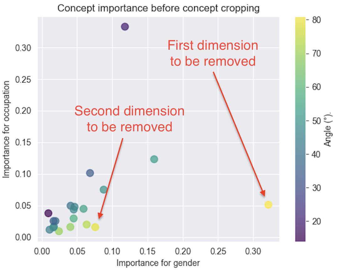
Figure 2: Co-importance plot for $r=20$ dimensions with respect to Occupation and Gender labels, computed with the Sobol method. The colour is based on the angle $a=90-\frac{2}{\pi}\arctan{(\frac{y}{x})}$. The angles with extreme values correspond to concepts with high importance for gender, but comparatively low importance for occupation. Their removal yields a favourable tradeoff in accuracy/fairness.

To estimate the importance of a concept $\bm{U}_{i}$ for gender (resp. for the label), we measure the fluctuations of the model output $c_{g}(\bm{U}\bm{W})$ (resp. $c(\bm{U}\bm{W})$) in response to perturbations of concept coefficient $\bm{U}_{i}$ .

We then propagate this perturbed activation to the model output $\bm{G}=c_{g}(\tilde{\bm{A}})$ (resp. $\bm{Y}=c(\tilde{\bm{A}})$). We can capture the importance that a concept might have as a main effect – along with its interactions with other concepts – on the model’s output by calculating the expected variance that would remain if all the concepts except the i were to be fixed. This yields the general definition of the total Sobol indices. An important concept will have a large variance in the model’s output, while an unused concept will barely change it.

We explain the total Sobol indices for each concept in details in Appendix E, along with our perturbation strategy.

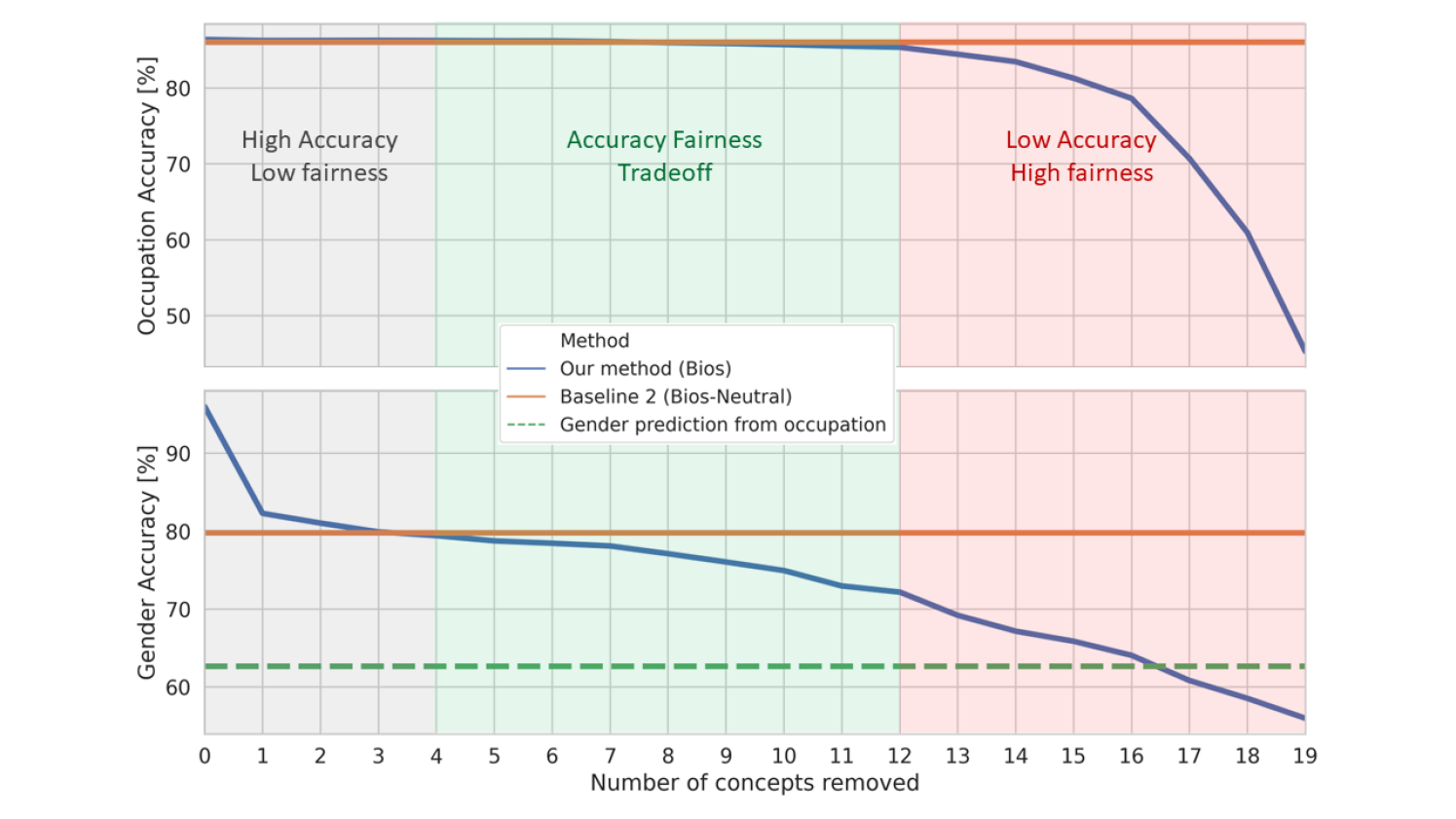
(a)

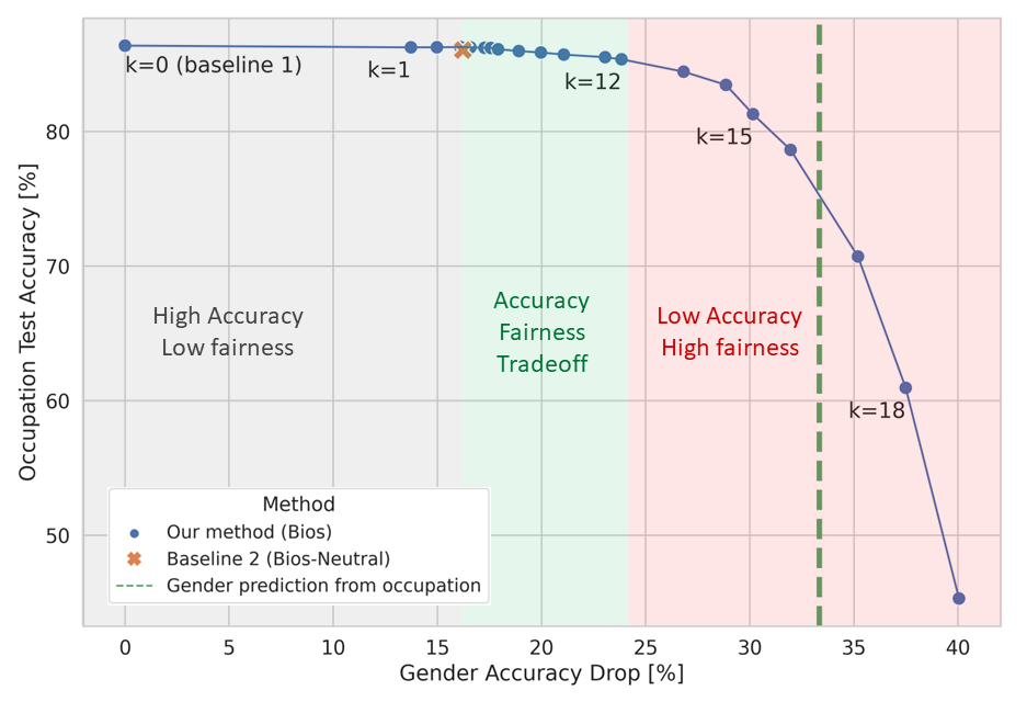
(b)

Figure 3: Accuracy drop when $k$ concepts are removed for an SVD with $r=20$ dimensions. In Figure 3(a), (Top) the occupation accuracy, (Bottom) the gender accuracy. Figure 3(b) shows occupation accuracy as a function of gender accuracy drop. The gender accuracy drop is reported relatively to the Baseline1, the classifier trained on Bios with all the concepts.

4.3 Neutralizing the embedding with importance-based concept removal

In this final section, we propose to eliminate $k$ concepts that exhibit significant gender dependence within the final embedding matrix, with the objective of improving its gender-neutrality. This provides us with an improved embedding which can serve as a base to learn a fairer classifier to predict downstream tasks, and thus, a more gender-neutral model overall.

This concept-removal procedure consists of choosing the $k$ concepts that maximize the ratio between the importance for gender prediction and for the task. This graphically corresponds to searching for the concepts whose angle with respect to the line of equal importance for gender and task prediction are the highest (see Fig. 2). This strategy allows us to work on a trade-off between the model’s performance and its fairness.

In practice, we sort the concepts $\bm{U}_{1}$,$\bm{U}_{2}$,….$\bm{U}_{r}$ according to the second strategy in descending order and we delete the $k$ first concepts. This essentially leaves us with a concept base $\tilde{\bm{U}}=(\bm{U}_{k+1},...,\bm{U}_{r})$. This same transformation can be applied to $\bm{W}$’s lines, yielding $\tilde{\bm{W}}$. From the matrix obtained from the matrix product $\tilde{\bm{U}}\tilde{\bm{W}}$, we retrain a classifier $\tilde{c}$ to predict $\bm{Y}$ (refer to Appendix C.2 for more details).

It is interesting to note that, because we are causally removing information from the latent space, it is impossible for any model to recover it from the truncated space – i.e. we are not limited by the family of models that’s intervening Ravfogel et al. (2023). Thus, we’re trading off the precision of the methods in the state-of-the-art Ravfogel et al. (2022); Belrose et al. (2023); Ravfogel et al. (2020); Shao et al. (2022, 2023) for interpretability of the removed information.

5 Results

5.1 Dataset and models

To illustrate our method, we use the Bios dataset De-Arteaga et al. (2019), which contains about 440K biographies (textual data) with labels for the genders (M or F) of the authors, and their occupations (28 classes). From the Bios dataset, we also create a second dataset Bios-neutral by removing all the explicit gender indicators. Bios-neutral will be used as a baseline to which we can compare our method. We leave the details of how this dataset preprocessing was performed in Appendix B.

For both datasets, we train a RoBERTa (Liu et al., 2019a) model to predict the occupation task. We leave the details on how these models were trained in Appendix C.

5.2 Results analysis - Quantitative part

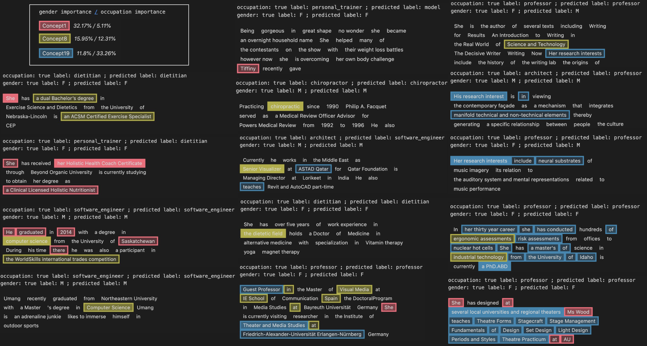
Figure 4: Understanding concepts extracted from the model trained on Bios. Concept 1 prominently features explicit gender indicators like ’she’ and ’his’, crucial for gender identification but irrelevant for occupation. Concept 8 integrates information about gender-unbalanced professions, aiding in predicting both, an individual’s gender and occupation. Concept 19 focuses on information related to the professor occupation, a gender-balanced class and most represented in the dataset.

Initially, we will examine the progression of our model’s performance for each dimension removed (one by one) utilizing our methodology.

Following the precepts of information theory, we will assess the effectiveness of our bias mitigation strategy by measuring the model’s capacity to predict the gender and the task as we progressively remove concepts.

We showcase in Fig. 3 the outcome of removing the $k$ most important concepts for $k\in\llbracket 0,19\rrbracket$ (we have $r=20$ dimensions) in terms of different metrics: accuracy on gender prediction and on predicting occupation (downstream task). We compare our technique to two baselines: Baseline1 – RoBERTa model trained on Bios dataset (i.e. when $k=0$) –, and Baseline2 – RoBERTa model trained on Bios-neutral dataset.

From Figure 3, simply by removing one concept, we achieve significant gains in the gender neutrality of our model, as it predicts gender with much lower accuracy (82.3% compared to the initial 96%) while maintaining its performance in occupation prediction (accuracy decreasing from 86.4% to 86.3%). Starting from the removal of the fourth dimension, the accuracy of gender prediction falls below the threshold of Baseline2, with 79.4% accuracy compared to 79.8% for Baseline2, while maintaining an accuracy of 86.3% for occupation (compared to 86% for Baseline2). Moreover, our method, in addition to being explainable, time-efficient, and cost-effective, exhibits greater effectiveness.

After removing these first four concepts, we enter a regime where removing concepts continues to gain us fairness (as the accuracy of the gender task continues to fall), while the accuracy of the occupation remains unchanged. This regime is therefore the one with the best trade-off between accuracy and fairness (shown in green here). From concept 12 onwards, the accuracy of occupation begins to decline, as we look more and more at concepts with a high importance for occupation (according to Sobol), and we enter a new regime where we gain more and more in fairness, but where the accuracy of our task collapses. It may be worthwhile deleting a fairly large number of concepts to get into this zone, but only if we are willing to pay the price in terms of prediction quality.

It is important to note that in this specific application, the optimal fairness-accuracy trade-off corresponds to accuracy on gender prediction of 62% as that’s the accuracy one gets when learning a model to predict the gender with the occupation labels as only information.

5.3 Concepts removed analysis - Explainability part

In this section, we interpret the dimensions of the Singular Value Decomposition (SVD) as valuable concepts for predicting our two tasks: gender and occupation. For this, we use the interpretability part of the COCKATIEL Jourdan et al. (2023) method on concepts/dimensions previously found with the SVD and ranked with the Sobol method by importance for gender and occupation.

Concept interpretability

COCKATIEL modifies the Occlusion method Zeiler and Fergus (2014), which operates by masking each word and subsequently observing the resultant impact on the model’s output. In this instance, to infer the significance of each word pertaining to a specific concept, words within a sentence are obscured, and the influence of the modified sentence (devoid of the words) on the concept is measured. This procedure can be executed at either the word or clause level, meaning it can obscure individual words or entire clauses, yielding explanations of varying granularity contingent upon the application.

Concepts interpretation

For the dimensions of the SVD to be meaningful for explanation, they must first be meaningful for the model’s prediction, whether it be the model predicting gender or the one predicting occupation. We rank the concepts w.r.t their removal order, and we focus on three important ones:
Concept 1, with a gender importance of 32%, and an occupation importance of 5%; Concept 8, with a gender importance of 16%, and an occupation importance of 12%; Concept 19, with a gender importance of 12%, and an occupation importance of 33%.

These three concepts are crucial for the prediction of at least one of our two tasks. Moreover, they are representative of our problem statement as Concept 1 is more important for gender, Concept 8 is as important to gender as occupation, and Concept 19 is more important for occupation. We illustrate several examples of explanations for these three concepts in Figure 4 to enable qualitative analysis.

According to the importance per dimension calculated in part 2 of our method, concept 1 is almost exclusively predictive of gender. The most significant words for the concept of this dimension are explicit indicators of traditional gender.

Concept 8 is capable of predicting both gender and occupation. Within its concept, we find examples of biographies predominantly related to unbalanced professions such as dietitian (92.8% women), chiropractor (26.8% women), software engineer (16.2% women), and model (83% women). It is logical that the concept allowing the prediction of these professions also enables the prediction of gender, as it is strongly correlated in these particular professions.

Concept 19, which strongly predicts occupation, focuses on biographies predicting professors (constituting more than 29.7% of all individuals). This class is gender-balanced (with 45.1% women), providing little information on gender.

6 Conclusion

In this paper, we introduced a method for neutralizing the presence of bias in transformer model’s embeddings in an interpretable and cost-efficient way through concept-based explainability. In this study, we present a method applied to gender-related information, yet inherently adaptable to other sensitive variables. Indeed, by removing concepts that are mostly influential for gender prediction, we obtain embeddings that rely considerably less on gender information for generating predictions, and at the same time, remain highly accurate at the task. Furthermore, by doing so via explainable AI, we perform interventions that can be easily interpreted by humans, and thus gain trust in the bias mitigation process and insights into what produced the bias in the first place. Finally, thanks to its low computation cost, it can be easily applied to pre-trained, fine-tuned and even embeddings accessed through inference APIs, thus allowing our method to be applied to any model in a post-hoc manner.

Limitations

Herein, we propose a novel approach that serves as a framework that can be applied to various concept extraction techniques and feature importance computation methods. This means that the SVD could be exchanged for other dimensionality reduction techniques (and thus, change the properties of the concept base and coefficients), or Shapley values could be preferred over Sobol indices for the relaxation on the independence assumption, for instance. In addition, our application was gender bias mitigation, but it could be applied to any other type of bias as long as the sensitive variable is available or can be estimated. Moreover, although the information about gender in the dataset is considered to be binary, we remind the reader that actual gender is non-binary, and as such, appropriate considerations must be taken in real-world applications. However, it is crucial to note that our method does not share this limitation, as it is designed to operate effectively with variables of multiple classes, including non-binary gender categorizations. This highlights the need for the NLP community to develop datasets that incorporate a non-binary gender variable, thereby reflecting real-world complexities and promoting inclusivity.

Appendix A Gender prediction with RoBERTa

In this section, we study the impact on gender prediction of removing explicit gender indicators with a transformer model. To do this, we train a model on a dataset and we train a model with the same architecture on modified version of the dataset where we remove the explicit gender indicators. We train these models to predict the gender and we compare both of these model’s accuracies.

In our example, we use the Bios dataset De-Arteaga et al. (2019), which contains about 400K biographies (textual data). For each biography, we have the gender (M or F) associated. We use each biography to predict the gender, and then we clean the dataset and we create a second dataset without the explicit gender indicators (following the protocol in Appendix B).

We train a RoBERTa model, as explained in Appendix C.1. Instead of training the model on the occupations, we place ourselves directly in the case where we train the RoBERTa to predict gender (with the same parameters). We train both models over 5 epochs.

In figure 5, we go from 99% accuracy for the baseline to 90% accuracy for the model trained on the dataset without explicit gender indicators. Even with a dataset without explicit gender indicators, a model like RoBERTa performs well on the gender prediction task.

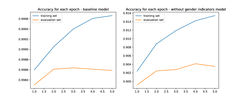
Figure 5: Convergence curves (accuracy) during training for the gender classification task, 5 epochs. (On the left) RoBERTa model trained on Bios; (On the right): RoBERTa model trained on Bios without explicit gender indicators.

Appendix B Dataset pre-processing protocol

We use Bios dataset De-Arteaga et al. (2019), which contains about 400K biographies (textual data). For each biography, Bios specifies the gender (M or F) of its author as well as its occupation (among a total of 28 possible occupations, categorical data).

As shown in Figure 6, this dataset contains heterogeneously represented occupations. Although the representation of some occupations is relatively well-balanced between males and females, other occupations are particularly unbalanced (see Figure 7).

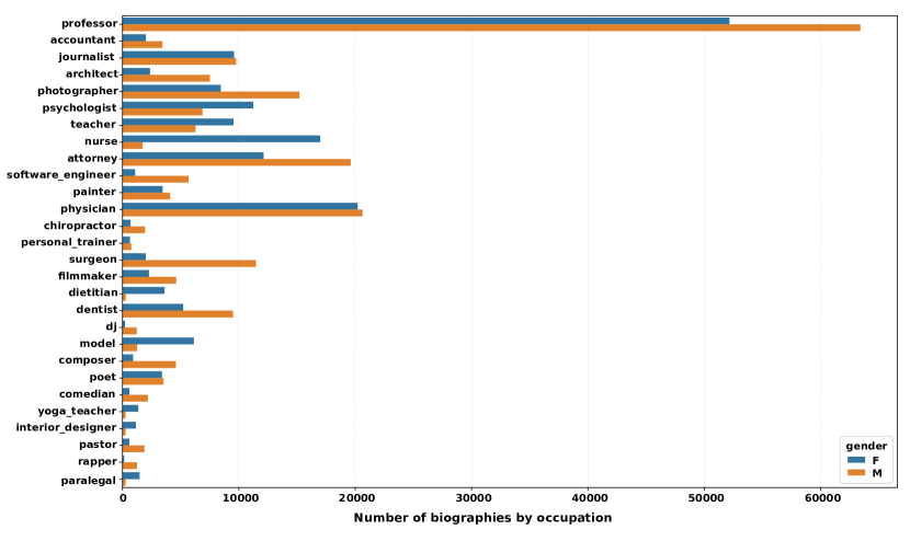
Figure 6: Number of biographies for each occupation by gender on the total Bios dataset De-Arteaga et al. (2019).

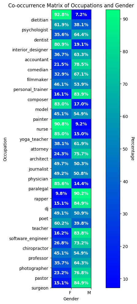
Figure 7: Co-occurrence of occupation and gender for Bios dataset De-Arteaga et al. (2019). Solely predicting the gender from the occupation yields a minimum of 62% accuracy, which is the minimum baseline for an accurate but unbiased model. Any classifier with lower accuracy on gender prediction must have accuracy on occupation prediction lower than $100\%$.

Cleaning dataset

To clean the dataset, we take all biographies and apply these modifications:

• we remove mail and URL,

• we remove dot after pronouns and acronyms,

• we remove double "?", "!" and ".",

• we cut all the biographies at 512 tokens by checking that they are cut at the end of a sentence and not in the middle.

Creating the Bios-neutral dataset

From Bios, we create a new dataset without explicit gender indicators, called Bios-neutral.

At first, we tokenize the dataset, then:

• If the token is a first name, we replace it with "Sam" (a common neutral first name).

• If the token is a dictionary key (on the dictionary defined below), we replace it with its values.

To determine whether the token is a first name, we use the list of first names: usna.edu

The dictionary used in the second part is based on the one created in Field and Tsvetkov (2020).

Appendix C Models details and convergence curves

C.1 RoBERTa training

RoBERTa base training

We use a RoBERTa model (Liu et al., 2019a), which is based on the transformers architecture and is pretrained with the Masked language modelling (MLM) objective. We specifically used a RoBERTa base model pretrained by Hugging Face. All information related to how it was trained can be found in Liu et al. (2019b). It can be remarked, that a very large training dataset was used to pretrain the model, as it was composed of five datasets: BookCorpus Zhu et al. (2015), a dataset containing 11,038 unpublished books; English Wikipedia (excluding lists, tables and headers); CC-News Mackenzie et al. (2020) which contains 63 millions English news articles crawled between September 2016 and February 2019; OpenWebText Radford et al. (2019) an open-source recreation of the WebText dataset used to train GPT-2; Stories Trinh and Le (2018) a dataset containing a subset of CommonCrawl data filtered to match the story-like style of Winograd schemas. Pre-training was performed on these data by randomly masking 15% of the words in each of the input sentences and then trying to predict the masked words.

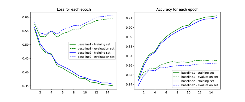
Figure 8: Convergence curves during training for occupation classification task, 15 epochs. Baseline1: RoBERTa model trained on Bios; Baseline2: RoBERTa model trained on Bios without explicit gender indicators. (On the left) accuracy curves; (on the right) loss curves.

Occupation prediction task

After pre-training RoBERTa parameters on this huge dataset, we then trained it on the 400.000 biographies of the Bios dataset. The training was performed with PyTorch on 2 GPUs (Nvidia Quadro RTX6000 24GB RAM) for 10 epochs (we train 15 epochs but we stop at 10 epochs) with a batch size of 8 observations and a sequence length of 512 words. The optimizer was Adam with a learning rate of 1e-6, $\beta_{1}=0.9$, $\beta_{2}=0.98$, and $\epsilon=1e6$. We split dataset into 70% for training, 10% for validation, and 20% for testing.

The convergence curves of the model are in Figure 8.

C.2 Classifier heads training

The importance estimation in part 2 of our method requires a classifier to be trained on top of the features. An ideal classifier will leverage the maximum amount possible of information about gender or occupation that can be realistically extracted from latent features, in the spirit of the maximum information that can be extracted under computational constraints Xu et al. (2020). Hence, it is crucial to optimize an expressive model to the highest possible performance.

In the latent space of the feature extractor, the decisions are usually computed with a linear classifier. However, when operating on latent space with removed concepts or when working with a task on which the transformer head has not been fine-tuned, nothing guarantees that the task can be solved with linear probes. Hence, we chose a more expressive model, namely a two-layer perceptron with ReLU non-linearities, and architecture $768\rightarrow 128\rightarrow C$ with $C$ the number of classes. The network is trained by minimizing the categorical cross-entropy on the train set, with Softmax activation to convert the logits into probabilities. We use Adam with a learning rate chosen between $10^{-5}$ and $10^{-1}$ with cross-validation on the validation set. Note that the paper reports the accuracy on the test set.

The gender classifier $c_{g}$ and the occupation classifer $\tilde{c}$ are both trained with this same protocol.

Appendix D Implementation details for SVD

We used the SVD implementation in sparse.linalg.svds provided in the Scipy package. This function makes use of an incremental strategy to only estimate the first singular vectors of $\bm{A}$, making the truncated SVD scalable to large matrices. Note that this implementation turned out to obtain the most robust decompositions of $\bm{A}$ after an empirical comparison between torch.svd, torch.linalg.svd, scipy.linalg.svd, and sklearn.decomposition.TruncatedSVD on our data.

Appendix E Sobol Indices - details

In this section, we define the classic Total Sobol indices and how they are calculated using our method. In practice, these indices can be calculated very efficiently Marrel et al. (2009); Saltelli et al. (2010); Janon et al. (2014) with Quasi-Monte Carlo sampling and the estimator explained below.

Let $(\Omega,\mathcal{A},\mathbb{P})$ be a probability space of possible concept perturbations. To build these concept perturbations, we use $\boldsymbol{M}=\left(M_{1},\ldots,M_{r}\right)\in\mathcal{M}\subseteq[0,1]^{r}$, i.i.d. stochastic masks where $M_{i}\sim\mathcal{U}(\left[0,1\right]),\forall i\in 1,...,r$. We define concept perturbation $\tilde{\bm{U}}=\boldsymbol{\pi}(\bm{U},\boldsymbol{M})$ with the perturbation operator $\boldsymbol{\pi}(\bm{U},\boldsymbol{M})=\bm{U}\odot\boldsymbol{M}$ with $\odot$ the Hadamard product (that takes in two matrices of the same dimensions and returns a matrix of the multiplied corresponding elements).

We denote the set $\mathcal{U}=\{1,\ldots,r\}$, $\boldsymbol{u}$ a subset of $\mathcal{U}$, its complementary $\sim\boldsymbol{u}$ and $\mathbb{E}(\cdot)$ the expectation over the perturbation space. We define $\phi:\mathcal{A}\rightarrow\mathbb{R}$, a function that takes the perturbations $\bm{U}$ from the last layer and applies the difference between the model’s two largest output logits – i.e. $\phi(\bm{U})=l_{(1)}(c(\bm{U}))-l_{(2)}(c(\bm{U}))$ where $c$ is the classification head of the model (when we do Sobol for the occupation task, it is $c$, and when we do Sobol for the gender task, it is $c_{g}$) and $l_{(1)}$ and $l_{(2)}$ represent the highest and second highest logit values respectively. We assume that $\phi\in\mathbb{L}^{2}(\mathcal{A},\mathbb{P})$ – i.e. $|\mathbb{E}(\phi(\boldsymbol{U}))|<+\infty$.

The Hoeffding decomposition provides $\phi$ as a function of summands of increasing dimension, denoting $\phi_{\boldsymbol{u}}$ the partial contribution of the concepts $\boldsymbol{U}_{\boldsymbol{u}}=\left(U_{i}\right)_{i\in\boldsymbol{u}}$ to the score $\phi(\boldsymbol{U})$:

$$\phi(\boldsymbol{U}) =\phi_{\varnothing}$$ (3)

$$+\sum_{i=1}^{r}\phi_{i}\left(U_{i}\right)$$

$$+\sum_{1\leqslant i<j\leqslant r}\phi_{i,j}\left(U_{i},U_{j}\right)+\cdots$$

$$+\phi_{1,\ldots,r}\left(U_{1},\ldots,U_{r}\right)$$

$$=\sum_{\boldsymbol{u}\subseteq\mathcal{U}}\phi_{\boldsymbol{u}}\left(\boldsymbol{U}_{\boldsymbol{u}}\right)$$

Eq. 3 consists of $2^{r}$ terms and is unique under the orthogonality constraint:

$$\quad\mathbb{E}\left(\phi_{\boldsymbol{u}}\left(\boldsymbol{U}_{\boldsymbol{u}}\right)\phi_{\boldsymbol{v}}\left(\boldsymbol{U}_{\boldsymbol{v}}\right)\right)=0,$$

$$\forall(\boldsymbol{u},\boldsymbol{v})\subseteq\mathcal{U}^{2}\text{ s.t. }\boldsymbol{u}\neq\boldsymbol{v}$$

Moreover, thanks to orthogonality, we have $\phi_{\boldsymbol{u}}\left(\boldsymbol{U}_{\boldsymbol{u}}\right)=\mathbb{E}\left(\phi(\boldsymbol{U})\mid\boldsymbol{U}_{\boldsymbol{u}}\right)-\sum_{\boldsymbol{v}\subset\boldsymbol{u}}\phi_{\boldsymbol{v}}\left(\boldsymbol{U}_{\boldsymbol{v}}\right)$ and we can write the model variance as:

$$\mathbb{V}(\phi(\boldsymbol{U})) =\sum_{i}^{r}\mathbb{V}\left(\phi_{i}\left(U_{i}\right)\right)$$ (4)

$$+\sum_{1\leqslant i<j\leqslant r}\mathbb{V}\left(\phi_{i,j}\left(U_{i},U_{j}\right)\right)$$

$$+\ldots+\mathbb{V}\left(\phi_{1,\ldots,r}\left(U_{1},\ldots,U_{r}\right)\right)$$

$$=\sum_{\boldsymbol{u}\subseteq\mathcal{U}}\mathbb{V}\left(\phi_{\boldsymbol{u}}\left(\boldsymbol{U}_{\boldsymbol{u}}\right)\right)$$

Eq. 4 allows us to write the influence of any subset of concepts $\boldsymbol{u}$ as its own variance. This yields, after normalization by $\mathbb{V}(\phi(\boldsymbol{U}))$, the general definition of Sobol’ indices.

Definition

Sobol’ indices Sobol (1993). The sensitivity index $\mathcal{S}_{\boldsymbol{u}}$ which measures the contribution of the concept set $\boldsymbol{U}_{\boldsymbol{u}}$ to the model response $f(\boldsymbol{U})$ in terms of fluctuation is given by:

$$\mathcal{S}_{\boldsymbol{u}}=\frac{\mathbb{V}\left(\phi_{\boldsymbol{u}}\left(\boldsymbol{U}_{\boldsymbol{u}}\right)\right)}{\mathbb{V}(\phi(\boldsymbol{U}))}=\\$$ (5)

$$\frac{\mathbb{V}\left(\mathbb{E}\left(\phi(\boldsymbol{U})\mid\boldsymbol{U}_{\boldsymbol{u}}\right)\right)-\sum_{\boldsymbol{v}\subset\boldsymbol{u}}\mathbb{V}\left(\mathbb{E}\left(\phi(\boldsymbol{U})\mid\boldsymbol{U}_{\boldsymbol{v}}\right)\right)}{\mathbb{V}(\phi(\boldsymbol{U}))}$$

Sobol’ indices provide a numerical assessment of the importance of various subsets of concepts in relation to the model’s decision-making process. Thus, we have: $\sum_{\boldsymbol{u}\subseteq\mathcal{U}}\mathcal{S}_{\boldsymbol{u}}=1$.

Additionally, the use of Sobol’ indices allows for the efficient identification of higher-order interactions between features. Thus, we can define the Total Sobol indices as the sum of of all the Sobol indices containing the concept $i:\mathcal{S}_{T_{i}}=\sum_{\boldsymbol{u}\subseteq\mathcal{U},i\in\boldsymbol{u}}\mathcal{S}_{\boldsymbol{u}}$. So we can write:

Definition

Total Sobol indices. The total Sobol index $\mathcal{S}{T_{i}}$, which measures the contribution of a concept $\bm{U}_{i}$ as well as its interactions of any order with any other concepts to the model output variance, is given by:

$$\mathcal{S}_{T_{i}} =\frac{\mathbb{E}_{\bm{M}_{\sim i}}(\mathbb{V}_{M_{i}}(\bm{Y}|\bm{M}_{\sim i}))}{\mathbb{V}(\bm{Y})}$$ (6)

$$=\frac{\mathbb{E}_{\bm{M}_{\sim i}}(\mathbb{V}_{M_{i}}(\phi((\bm{U}\odot\bm{M})\bm{W})|\bm{M}_{\sim i}))}{\mathbb{V}(\phi((\bm{U}\odot\bm{M})\bm{W}))}.$$ (7)

In practice, our implementation of this method remains close to what is done in COCKATIEL Jourdan et al. (2023), with the exception of changes to the $\phi$ function created here to manage concepts found in all the classes at the same time (unlike COCKATIEL, which concentrated on finding concepts in a per-class basis).

References

- Adebayo et al. (2018) Julius Adebayo, Justin Gilmer, Michael Muelly, Ian Goodfellow, Moritz Hardt, and Been Kim. 2018. Sanity checks for saliency maps. Advances in neural information processing systems, 31.
- Antognini and Faltings (2021) Diego Antognini and Boi Faltings. 2021. Rationalization through concepts. In Findings of the Association for Computational Linguistics: ACL-IJCNLP 2021, pages 761–775, Online. Association for Computational Linguistics.
- Asher et al. (2022) Nicholas Asher, Lucas De Lara, Soumya Paul, and Chris Russell. 2022. Counterfactual models for fair and adequate explanations. Machine Learning and Knowledge Extraction, 4(2):316–349.
- Asher et al. (2021) Nicholas Asher, Soumya Paul, and Chris Russell. 2021. Fair and adequate explanations. In International Cross-Domain Conference for Machine Learning and Knowledge Extraction, pages 79–97. Springer.
- Bastings et al. (2019) Jasmijn Bastings, Wilker Aziz, and Ivan Titov. 2019. Interpretable neural predictions with differentiable binary variables. arXiv preprint arXiv:1905.08160.
- Belrose et al. (2023) Nora Belrose, David Schneider-Joseph, Shauli Ravfogel, Ryan Cotterell, Edward Raff, and Stella Biderman. 2023. Leace: Perfect linear concept erasure in closed form. arXiv preprint arXiv:2306.03819.
- Bingham and Mannila (2001) Ella Bingham and Heikki Mannila. 2001. Random projection in dimensionality reduction: applications to image and text data. In Proceedings of the seventh ACM SIGKDD international conference on Knowledge discovery and data mining, pages 245–250.
- Bolukbasi et al. (2016) Tolga Bolukbasi, Kai-Wei Chang, James Y Zou, Venkatesh Saligrama, and Adam T Kalai. 2016. Man is to computer programmer as woman is to homemaker? debiasing word embeddings. Advances in neural information processing systems, 29.
- Caliskan et al. (2017) Aylin Caliskan, Joanna J Bryson, and Arvind Narayanan. 2017. Semantics derived automatically from language corpora contain human-like biases. Science, 356(6334):183–186.
- Comon (1994) Pierre Comon. 1994. Independent component analysis, a new concept? Signal processing, 36(3):287–314.
- De-Arteaga et al. (2019) Maria De-Arteaga, Alexey Romanov, Hanna Wallach, Jennifer Chayes, Christian Borgs, Alexandra Chouldechova, Sahin Geyik, Krishnaram Kenthapadi, and Adam Tauman Kalai. 2019. Bias in bios: A case study of semantic representation bias in a high-stakes setting. In proceedings of the Conference on Fairness, Accountability, and Transparency, pages 120–128.
- Devlin et al. (2018) Jacob Devlin, Ming-Wei Chang, Kenton Lee, and Kristina Toutanova. 2018. Bert: Pre-training of deep bidirectional transformers for language understanding. arXiv preprint arXiv:1810.04805.
- Dorleon et al. (2022) Ginel Dorleon, Imen Megdiche, Nathalie Bricon-Souf, and Olivier Teste. 2022. Feature selection under fairness constraints. In Proceedings of the 37th ACM/SIGAPP Symposium on Applied Computing, SAC ’22, page 1125–1127, New York, NY, USA. Association for Computing Machinery.
- Eckart and Young (1936) C. Eckart and G. Young. 1936. The approximation of one matrix by another of lower rank. Psychometrika, 1:211–218.
- Fel et al. (2023) Thomas Fel, Agustin Picard, Louis Bethune, Thibaut Boissin, David Vigouroux, Julien Colin, Rémi Cadène, and Thomas Serre. 2023. Craft: Concept recursive activation factorization for explainability. In Proceedings of the IEEE/CVF Conference on Computer Vision and Pattern Recognition, pages 2711–2721.
- Ferrando et al. (2023) Javier Ferrando, Gerard I Gállego, Ioannis Tsiamas, and Marta R Costa-jussà. 2023. Explaining how transformers use context to build predictions. arXiv preprint arXiv:2305.12535.
- Field and Tsvetkov (2020) Anjalie Field and Yulia Tsvetkov. 2020. Unsupervised discovery of implicit gender bias. arXiv preprint arXiv:2004.08361.
- Frye et al. (2020) Christopher Frye, Colin Rowat, and Ilya Feige. 2020. Asymmetric shapley values: incorporating causal knowledge into model-agnostic explainability. Advances in Neural Information Processing Systems, 33:1229–1239.
- Galhotra et al. (2022) Sainyam Galhotra, Karthikeyan Shanmugam, Prasanna Sattigeri, and Kush R. Varshney. 2022. Causal feature selection for algorithmic fairness. In Proceedings of the 2022 International Conference on Management of Data, SIGMOD ’22, page 276–285, New York, NY, USA. Association for Computing Machinery.
- Garg et al. (2018) Nikhil Garg, Londa Schiebinger, Dan Jurafsky, and James Zou. 2018. Word embeddings quantify 100 years of gender and ethnic stereotypes. Proceedings of the National Academy of Sciences, 115(16):E3635–E3644.
- Ghorbani et al. (2019) Amirata Ghorbani, Abubakar Abid, and James Zou. 2019. Interpretation of neural networks is fragile. In Proceedings of the AAAI conference on artificial intelligence, volume 33, pages 3681–3688.
- Gonen and Goldberg (2019) Hila Gonen and Yoav Goldberg. 2019. Lipstick on a pig: Debiasing methods cover up systematic gender biases in word embeddings but do not remove them. arXiv preprint arXiv:1903.03862.
- Ignatiev et al. (2019) Alexey Ignatiev, Nina Narodytska, and Joao Marques-Silva. 2019. On validating, repairing and refining heuristic ml explanations. arXiv preprint arXiv:1907.02509.
- Jacovi and Goldberg (2020) Alon Jacovi and Yoav Goldberg. 2020. Towards faithfully interpretable nlp systems: How should we define and evaluate faithfulness? In Proceedings of the 58th Annual Meeting of the Association for Computational Linguistics, pages 4198–4205.
- Jacovi et al. (2021) Alon Jacovi, Swabha Swayamdipta, Shauli Ravfogel, Yanai Elazar, Yejin Choi, and Yoav Goldberg. 2021. Contrastive explanations for model interpretability. In Proceedings of the 2021 Conference on Empirical Methods in Natural Language Processing, pages 1597–1611.
- Jain et al. (2020) Sarthak Jain, Sarah Wiegreffe, Yuval Pinter, and Byron C Wallace. 2020. Learning to faithfully rationalize by construction. arXiv preprint arXiv:2005.00115.
- Janon et al. (2014) Alexandre Janon, Thierry Klein, Agnes Lagnoux, Maëlle Nodet, and Clémentine Prieur. 2014. Asymptotic normality and efficiency of two sobol index estimators. ESAIM: Probability and Statistics, 18:342–364.
- Jourdan et al. (2023) Fanny Jourdan, Agustin Picard, Thomas Fel, Laurent Risser, Jean Michel Loubes, and Nicholas Asher. 2023. Cockatiel: Continuous concept ranked attribution with interpretable elements for explaining neural net classifiers on nlp tasks. arXiv preprint arXiv:2305.06754.
- Karita et al. (2019) Shigeki Karita, Nanxin Chen, Tomoki Hayashi, Takaaki Hori, Hirofumi Inaguma, Ziyan Jiang, Masao Someki, Nelson Enrique Yalta Soplin, Ryuichi Yamamoto, Xiaofei Wang, et al. 2019. A comparative study on transformer vs rnn in speech applications. In 2019 IEEE Automatic Speech Recognition and Understanding Workshop (ASRU), pages 449–456. IEEE.
- Kilbertus et al. (2017) Niki Kilbertus, Mateo Rojas Carulla, Giambattista Parascandolo, Moritz Hardt, Dominik Janzing, and Bernhard Schölkopf. 2017. Avoiding discrimination through causal reasoning. Advances in neural information processing systems, 30.
- Kim et al. (2018) Been Kim, Martin Wattenberg, Justin Gilmer, Carrie Cai, James Wexler, Fernanda Viegas, et al. 2018. Interpretability beyond feature attribution: Quantitative testing with concept activation vectors (tcav). In International conference on machine learning, pages 2668–2677. PMLR.
- Lei et al. (2016) Tao Lei, Regina Barzilay, and Tommi Jaakkola. 2016. Rationalizing neural predictions. arXiv preprint arXiv:1606.04155.
- Lewis (1973) David Lewis. 1973. Counterfactuals. Basil Blackwell, Oxford.
- Liang et al. (2020) Paul Pu Liang, Irene Mengze Li, Emily Zheng, Yao Chong Lim, Ruslan Salakhutdinov, and Louis-Philippe Morency. 2020. Towards debiasing sentence representations. arXiv preprint arXiv:2007.08100.
- Liu et al. (2019a) Yinhan Liu, Myle Ott, Naman Goyal, Jingfei Du, Mandar Joshi, Danqi Chen, Omer Levy, Mike Lewis, Luke Zettlemoyer, and Veselin Stoyanov. 2019a. Roberta: A robustly optimized bert pretraining approach. arXiv preprint arXiv:1907.11692.
- Liu et al. (2019b) Yinhan Liu, Myle Ott, Naman Goyal, Jingfei Du, Mandar Joshi, Danqi Chen, Omer Levy, Mike Lewis, Luke Zettlemoyer, and Veselin Stoyanov. 2019b. Roberta: A robustly optimized BERT pretraining approach. CoRR, abs/1907.11692.
- Mackenzie et al. (2020) Joel Mackenzie, Rodger Benham, Matthias Petri, Johanne R. Trippas, J. Shane Culpepper, and Alistair Moffat. 2020. Cc-news-en: A large english news corpus. In Proceedings of the 29th ACM International Conference on Information amp; Knowledge Management, CIKM ’20, page 3077–3084, New York, NY, USA. Association for Computing Machinery.
- Marques-Silva (2023) Joao Marques-Silva. 2023. Disproving xai myths with formal methods–initial results. arXiv preprint arXiv:2306.01744.
- Marrel et al. (2009) Amandine Marrel, Bertrand Iooss, Beatrice Laurent, and Olivier Roustant. 2009. Calculations of sobol indices for the gaussian process metamodel. Reliability Engineering & System Safety, 94(3):742–751.
- Pearl (2009) Judea Pearl. 2009. Causality. Cambridge university press.
- Petsiuk et al. (2018) Vitali Petsiuk, Abir Das, and Kate Saenko. 2018. Rise: Randomized input sampling for explanation of black-box models. arXiv preprint arXiv:1806.07421.
- Radford et al. (2019) Alec Radford, Jeffrey Wu, Rewon Child, David Luan, Dario Amodei, Ilya Sutskever, et al. 2019. Language models are unsupervised multitask learners. OpenAI blog, 1(8):9.
- Ravfogel et al. (2020) Shauli Ravfogel, Yanai Elazar, Hila Gonen, Michael Twiton, and Yoav Goldberg. 2020. Null it out: Guarding protected attributes by iterative nullspace projection. arXiv preprint arXiv:2004.07667.
- Ravfogel et al. (2023) Shauli Ravfogel, Yoav Goldberg, and Ryan Cotterell. 2023. Log-linear guardedness and its implications. In Proceedings of the 61st Annual Meeting of the Association for Computational Linguistics (Volume 1: Long Papers), pages 9413–9431.
- Ravfogel et al. (2022) Shauli Ravfogel, Michael Twiton, Yoav Goldberg, and Ryan D Cotterell. 2022. Linear adversarial concept erasure. In International Conference on Machine Learning, pages 18400–18421. PMLR.
- Ribeiro et al. (2016) Marco Tulio Ribeiro, Sameer Singh, and Carlos Guestrin. 2016. " why should i trust you?" explaining the predictions of any classifier. In Proceedings of the 22nd ACM SIGKDD international conference on knowledge discovery and data mining, pages 1135–1144.
- Rudin (2019) Cynthia Rudin. 2019. Stop explaining black box machine learning models for high stakes decisions and use interpretable models instead. Nature machine intelligence, 1(5):206–215.
- Saltelli et al. (2010) Andrea Saltelli, Paola Annoni, Ivano Azzini, Francesca Campolongo, Marco Ratto, and Stefano Tarantola. 2010. Variance based sensitivity analysis of model output. design and estimator for the total sensitivity index. Computer physics communications, 181(2):259–270.
- Shao et al. (2022) Shun Shao, Yftah Ziser, and Shay B Cohen. 2022. Gold doesn’t always glitter: Spectral removal of linear and nonlinear guarded attribute information. arXiv preprint arXiv:2203.07893.
- Shao et al. (2023) Shun Shao, Yftah Ziser, and Shay B Cohen. 2023. Erasure of unaligned attributes from neural representations. Transactions of the Association for Computational Linguistics, 11:488–510.
- Smilkov et al. (2017) Daniel Smilkov, Nikhil Thorat, Been Kim, Fernanda Viégas, and Martin Wattenberg. 2017. Smoothgrad: removing noise by adding noise. arXiv preprint arXiv:1706.03825.
- Sobol (1993) Ilya M Sobol. 1993. Sensitivity analysis for non-linear mathematical models. Mathematical modelling and computational experiment, 1:407–414.
- Sundararajan et al. (2017) Mukund Sundararajan, Ankur Taly, and Qiqi Yan. 2017. Axiomatic attribution for deep networks. In International conference on machine learning, pages 3319–3328. PMLR.
- Trinh and Le (2018) Trieu H Trinh and Quoc V Le. 2018. A simple method for commonsense reasoning. arXiv preprint arXiv:1806.02847.
- Vaswani et al. (2017) Ashish Vaswani, Noam Shazeer, Niki Parmar, Jakob Uszkoreit, Llion Jones, Aidan N Gomez, Łukasz Kaiser, and Illia Polosukhin. 2017. Attention is all you need. Advances in neural information processing systems, 30.
- Wang et al. (2020) Junlin Wang, Jens Tuyls, Eric Wallace, and Sameer Singh. 2020. Gradient-based analysis of nlp models is manipulable. arXiv preprint arXiv:2010.05419.
- Wiegreffe and Pinter (2019) Sarah Wiegreffe and Yuval Pinter. 2019. Attention is not not explanation. In Proceedings of the 2019 Conference on Empirical Methods in Natural Language Processing and the 9th International Joint Conference on Natural Language Processing (EMNLP-IJCNLP), pages 11–20.
- Wold et al. (1987) Svante Wold, Kim Esbensen, and Paul Geladi. 1987. Principal component analysis. Chemometrics and intelligent laboratory systems, 2(1-3):37–52.
- Xu et al. (2020) Yilun Xu, Shengjia Zhao, Jiaming Song, Russell Stewart, and Stefano Ermon. 2020. A theory of usable information under computational constraints. In International Conference on Learning Representations.
- Yin and Neubig (2022) Kayo Yin and Graham Neubig. 2022. Interpreting language models with contrastive explanations. In Proceedings of the 2022 Conference on Empirical Methods in Natural Language Processing, pages 184–198.
- Zeiler and Fergus (2014) Matthew D Zeiler and Rob Fergus. 2014. Visualizing and understanding convolutional networks. In European conference on computer vision, pages 818–833. Springer.
- Zhao et al. (2019) Jieyu Zhao, Tianlu Wang, Mark Yatskar, Ryan Cotterell, Vicente Ordonez, and Kai-Wei Chang. 2019. Gender bias in contextualized word embeddings. arXiv preprint arXiv:1904.03310.
- Zhao et al. (2018a) Jieyu Zhao, Tianlu Wang, Mark Yatskar, Vicente Ordonez, and Kai-Wei Chang. 2018a. Gender bias in coreference resolution: Evaluation and debiasing methods. arXiv preprint arXiv:1804.06876.
- Zhao et al. (2018b) Jieyu Zhao, Yichao Zhou, Zeyu Li, Wei Wang, and Kai-Wei Chang. 2018b. Learning gender-neutral word embeddings. arXiv preprint arXiv:1809.01496.
- Zhu et al. (2015) Yukun Zhu, Ryan Kiros, Richard Zemel, Ruslan Salakhutdinov, Raquel Urtasun, Antonio Torralba, and Sanja Fidler. 2015. Aligning books and movies: Towards story-like visual explanations by watching movies and reading books. In arXiv preprint arXiv:1506.06724.