N³LL resummation of one-jettiness for $Z$-boson plus jet
production at hadron colliders

Abstract

We present the resummation of one-jettiness for the colour-singlet plus jet production process $pp\to(\gamma^{*}/Z\to\ell^{+}\ell^{-})+{\text{jet}}$ at hadron colliders up to the fourth logarithmic order (N³LL). This is the first resummation at this order for processes involving three coloured partons at the Born level. We match our resummation formula to the corresponding fixed-order predictions, extending the validity of our results to regions of the phase space where further hard emissions are present. This result paves the way for the construction of next-to-next-to-leading order simulations for colour-singlet plus jet production matched to parton showers in the Geneva framework.

I Introduction

The study of the production of a colour singlet system at large recoil is of crucial importance for the physics programme at the Large Hadron Collider. In particular, theoretical predictions for $\gamma^{*}/Z+$jet production are needed at higher precision to match the accuracy reached by experimental measurements of the $Z$ boson transverse momentum ($q_{T}$) spectrum. Combining next-to-next-to-leading order (NNLO) predictions for $\gamma^{*}/Z+$jet [1, 2, 3, 4, 5, 6] with $q_{T}$ resummation [7, 8, 9, 10, 11, 12, 13, 14] provides an accurate description of this distribution over the whole kinematic range and can be used to extract $\alpha_{s}$ [15] and as a background for new physics searches.

The one-jettiness variable is a suitable event shape for colour singlet ($L$) + jet production which does not suffer from superleading or nonglobal logarithms. It is a specific case of $N$-jettiness [16], and has been used to perform slicing calculations at NNLO [17, 18, 19, 20, 21]. Resummation of the jettiness has been performed for various $N$ [22, 23, 24, 25], and this was exploited to match NNLO calculations to parton shower algorithms for colour singlet production in Geneva [22, 26, 23, 27, 28, 29, 30]. In this work, we resum the one-jettiness up to N³LL accuracy, providing state-of-the-art predictions for this variable, which was only previously known up to NNLL [24]. In order to obtain this accurate result, we rely on higher-order perturbative ingredients which have only become available in the last few years. In particular, the structure of the hard anomalous dimensions that is relevant for N³LL resummation was derived in ref. [31] together with the direct evaluation of the four-loop cusp anomalous dimension in ref. [32, 33]. N³LL resummation also requires the knowledge of two-loop soft boundary terms which were first evaluated in ref. [34, 35] and recomputed for this paper with a refined treatment of the small and large angle regions [36].

We define the one-jettiness resolution variable as [16]

$$\mathcal{T}_{1}=\sum_{k}\min\bigg{\{}\frac{2q_{a}\cdot p_{k}}{Q_{a}},\frac{2q_{b}\cdot p_{k}}{Q_{b}},\frac{2q_{J}\cdot p_{k}}{Q_{J}}\bigg{\}}\,,$$ (1)

with $q_{a,b}=x_{a,b}E_{\mathrm{cm}}\,n_{a,b}/2=E_{a,b}\,n_{a,b}$ and $q_{J}=E_{J}\,n_{J}$, where $E_{J}$ is the jet energy. The beam directions are $n_{a,b}=(1,0,0,\pm 1)$ while the massless jet direction is $n_{J}=(1,\vec{n}_{J})$. In eq. (1) the sum runs over the four-momenta $p_{k}$ of all partons which are part of the hadronic final state. We use a geometric measure where $Q_{i}=2\rho_{i}E_{i}$ with $i=a,b,J$ is proportional to the energy of the beam or jet momenta. This particular choice is preferable because it is independent of the total jet energy, but makes the one-jettiness definition frame dependent. Results in frames that differ by a longitudinal boost can be obtained by making different choices for $\rho_{i}$. In this work we show results for $\mathcal{T}_{1}$ in the laboratory frame (LAB) and in the frame where the colour singlet system has zero rapidity (CS). The LAB frame definition is obtained by setting $\rho_{i}=1$ and evaluating the jet energy and the directions of the partonic momenta in the laboratory. In order to obtain the CS frame definition we instead set

$$\rho_{a}=e^{\hat{Y}_{L}},\,\rho_{b}=e^{-\hat{Y}_{L}},\,\rho_{J}=(e^{-\hat{Y}_{L}}\hat{q}_{J}^{+}+e^{\hat{Y}_{L}}\hat{q}_{J}^{-})/(2\hat{E}_{J}),$$

where $\hat{Y}_{L}$ is the rapidity of $L$ in the laboratory. The quantities $\hat{q}_{J}^{\pm}=\hat{q}_{J}^{0}\mp\hat{q}_{J}^{3}$ and $\hat{E}_{J}$ are the lightcone components and energy of the reconstructed massless jet four-momentum $\hat{q}_{J}$ in the laboratory frame respectively. In this way the longitudinal boost between the two frames is absorbed by a redefinition of the $\rho_{i}$.

The manuscript is organised as follows. In sec. II we introduce the factorisation formula, detailing its ingredients and their renormalisation group (RG) evolution. We present a final resummed formula valid up to N³LL accuracy and we match it with the appropriate fixed-order calculation in order to extend the description of the one-jettines spectrum also in regions where more than one hard jet is present. In sec. III we discuss the details of the implementation and present our results for the one-jettiness distribution. We also study the nonsingular contribution in different frames and provide predictions matched to the appropriate fixed-order (FO) distributions. We finally draw our conclusions in sec. IV. Further details about the derivation of the resummed results are described in the appendices.

II Factorisation and Resummation

A general factorisation formula for the $N$-jettiness distribution was derived in ref. [37, 38]. For the case of one-jettiness in hadronic collisions it reads

$$\frac{\mathrm{d}\sigma}{\mathrm{d}\Phi_{1}\mathrm{d}\mathcal{T}_{1}}\!=\! \sum_{\kappa}H_{\kappa}(\Phi_{1},\mu)\int\,\mathrm{d}t_{a}\,\mathrm{d}t_{b}\,\mathrm{d}s_{J}$$ (2)

$$\ \times\ B_{\kappa_{a}}(t_{a},x_{a},\mu)\ B_{\kappa_{b}}(t_{b},x_{b},\mu)\ J_{\kappa_{J}}(s_{J},\mu)$$

$$\ \times\ S_{\kappa}\left(n_{a}\cdot n_{J},\mathcal{T}_{1}-\frac{t_{a}}{Q_{a}}-\frac{t_{b}}{Q_{b}}-\frac{s_{J}}{Q_{J}},\mu\right)\,,$$

where $x_{a,b}=(Q_{LJ}/E_{\mathrm{cm}})\exp\{\pm Y_{LJ}\}$ and $Q_{LJ}$ is the invariant mass of the colour-singlet plus jet system ($LJ$). The index set $\kappa\equiv\{\kappa_{a},\kappa_{b},\kappa_{J}\}$ runs over all allowed partonic channels and $\kappa_{a}$, $\kappa_{b}$, $\kappa_{J}$ denote the individual parton types. $\Phi_{1}$ is the phase space for the $LJ$ system and $n_{a}\cdot n_{J}=(1-\cos\theta_{aJ})$ measures the angle between the jet and the rightward beam direction in the laboratory frame. In general, for $L$+jet production all permitted partonic channels contribute, i.e. $\kappa_{a}\,\kappa_{b}\,\kappa_{J}\in\{q\bar{q}g,qgq,ggg,\ldots\}$, where we have indicated all the crossing and charge-conjugated processes within the dots. For the $pp\to(\gamma^{*}/Z\to\ell^{+}\ell^{-})+{\text{jet}}+X$ case we consider in this work, the $q\bar{q}g$ and $qgq$ channels (plus their crossing and charge-conjugated ones) appear at Born level. The $ggg$ channel instead begins to contribute only at $\mathcal{O}(\alpha_{s}^{3})$.

In eq. (2) the hard functions $H_{\kappa}$ are defined as the square of the Wilson coefficients of the effective theory operators defined in Soft-Collinear Effective Theory (SCET). They can be obtained from the UV- and IR-finite relevant amplitudes in full QCD. The beam $B_{\kappa_{a/b}}$ and the jet $J_{\kappa_{J}}$ functions describe collinear emissions along the beam and jet directions respectively. The functions $S_{\kappa}$ describe isotropic soft emissions from soft Wilson lines and depend on the angle between the beam and jet directions.

When the hard, soft, beam and jet functions are evaluated at a common scale $\mu$, large logarithms of the ratios of disparate scales may arise, which spoil the convergence of fixed-order perturbation theory. The resummation of such logarithms is achieved through RG evolution in the SCET framework. All the functions appearing in the factorisation formula are evolved from their characteristic energy scales ($\mu_{X},\,X=H,S,B,J$) to the common scale $\mu$ by separately solving their associated RG evolution equations. The accuracy of the resummed predictions is systematically improvable by including higher-order terms in the fixed-order expansions of the hard, soft, beam and jet functions as well as in their corresponding anomalous dimensions. To achieve N³LL accuracy one needs the boundary conditions of the hard, soft, beam and jet functions up to two loops. The coefficients of the scale-dependent and kinematic-dependent logarithmic terms in the anomalous dimension and the QCD beta function need to be evaluated up to four loops. Finally, nonlogarithmic noncusp terms in the anomalous dimension need to be evaluated up to three loops.

In the rest of this section we will present the functions appearing in the factorisation formula (2) and their evolution separately and derive the final resummed formula in sec. II.4.

II.1 Hard functions for $pp\to(\gamma^{*}/Z\to\ell^{+}\ell^{-})+{\text{jet}}$

The hard function for the channel $\kappa$ satisfies the following RG equation (RGE)

$$\frac{\mathrm{d}}{\mathrm{d}\log\mu}H_{\kappa}(\Phi_{1},\mu) =\Gamma_{H}^{\kappa}(\mu)\,H_{\kappa}(\Phi_{1},\mu)\,,$$ (3)

with $\Gamma^{\kappa}_{H}(\mu)=2\mathrm{Re}\,\{\Gamma^{\kappa}_{C}(\mu)\}$. Here we have already exploited the fact that for the colour-singlet plus jet production process, the colour structure is trivial, i.e. the anomalous dimensions of the Wilson coefficient $\Gamma^{\kappa}_{C}(\mu)$ (or equivalently the anomalous dimension of the hard function $\Gamma^{\kappa}_{H}(\mu)$) is diagonal in colour space, as we show below. For ease of notation we use in this section the abbreviations $a=\kappa_{a}$, $b=\kappa_{b}$ and $c=\kappa_{J}$. Writing the anomalous dimension $\Gamma^{\kappa}_{C}(\mu)$ in full generality as a matrix in colour space and using its explicit expression up to N³LL given in ref. [31], we find

$$\boldsymbol{\Gamma}_{C}^{\kappa}(\mu) =\Gamma_{C}^{\kappa}(\mu)\ \boldsymbol{1}\ =\bigg{\{}\frac{\Gamma_{\mathrm{cusp}}(\alpha_{s})}{2}\bigg{[}\big{(}C_{c}-C_{a}-C_{b}\big{)}\ln\frac{\mu^{2}}{(-s_{ab}-\mathrm{i}0)}+\textrm{cyclic permutations}\bigg{]}$$

$$\quad+\gamma^{a}_{C}(\alpha_{s})+\gamma_{C}^{b}(\alpha_{s})+\gamma_{C}^{c}(\alpha_{s})+{{\frac{C^{2}_{A}}{8}}}f(\alpha_{s})\big{(}C_{a}+C_{b}+C_{c}\big{)}\bigg{\}}\boldsymbol{1}$$

$$\quad+\sum_{(i,j)}\bigg{[}-f(\alpha_{s})\mathbfcal{T}_{iijj}+\sum_{R=F,A}g^{R}(\alpha_{s})\big{(}3\mathbfcal{D}^{R}_{iijj}+4\mathbfcal{D}^{R}_{iiij}\big{)}\ln\frac{\mu^{2}}{(-s_{ij}-\mathrm{i}0)}\bigg{]}+\mathcal{O}(\alpha_{s}^{5})\,,$$ (4)

where the sums run over all the external hard parton pairs with $i\neq j$ and $C_{i}$ is the quadratic Casimir invariant for the parton $i$ in the colour representation $R_{i}$. The symbol ‘$\boldsymbol{1}$’ denotes the identity element in colour space. The cusp $\Gamma_{\mathrm{cusp}}(\alpha_{s})$ and noncusp $\gamma^{i}_{C}(\alpha_{s})$ anomalous dimensions are given in App. A of ref. [31] for both quark and gluon cases. We have $\Gamma_{\mathrm{cusp}}(\alpha_{s})=\sum_{n=0}^{\infty}\left(\frac{\alpha_{s}}{4\pi}\right)^{n}\Gamma_{n}$, with $\Gamma_{n}$ the universal cusp anomalous dimension coefficients. The symmetrised colour structures that appear in eq. (II.1) are defined as

$$\mathbfcal{T}_{ijkl} =f^{ade}f^{bce}(\boldsymbol{T}^{a}_{i}\boldsymbol{T}^{b}_{j}\boldsymbol{T}^{c}_{k}\boldsymbol{T}^{d}_{l})_{+}\,,$$

$$\mathbfcal{D}^{R}_{ijkl} =d^{abcd}_{R}\boldsymbol{T}^{a}_{i}\boldsymbol{T}^{b}_{j}\boldsymbol{T}^{c}_{k}\boldsymbol{T}^{d}_{l}\,,$$ (5)

where $\big{(}\boldsymbol{T}^{a_{1}}_{i_{1}}\ldots\boldsymbol{T}^{a_{n}}_{i_{n}}\big{)}_{+}\equiv\frac{1}{n!}\sum_{\pi}\boldsymbol{T}^{a_{\pi(a)}}_{i_{\pi(1)}}\ldots\boldsymbol{T}^{a_{\pi(n)}}_{i_{\pi(n)}}$ denotes the normalised sum of all possible permutations $\pi$ of the $n$ colour operators and

$$d^{a_{1}\ldots a_{n}}_{R} =\mathrm{Tr}_{R}(\boldsymbol{T}^{a_{1}}\ldots\boldsymbol{T}^{a_{n}})_{+}$$

$$=\frac{1}{n!}\sum_{\pi}\mathrm{Tr}\big{(}\boldsymbol{T}^{a_{\pi(1)}}_{R}\ldots\boldsymbol{T}^{a_{\pi(n)}}_{R}\big{)}\,.$$ (6)

The functions $f(\alpha_{s})$ and $g^{R}(\alpha_{s})$ ($R=F$ for the fundamental and $R=A$ for the adjoint representation) start at $\mathcal{O}(\alpha_{s}^{3})$ and $\mathcal{O}(\alpha_{s}^{4})$ respectively. The explicit expressions can be derived from ref. [31, 32, 33]; we report them below for completeness

$$f(\alpha_{s})= \ 16\,\big{(}\,\zeta_{5}+2\zeta_{2}\zeta_{3}\,\big{)}\,\left(\frac{\alpha_{s}}{4\pi}\right)^{3}+\mathcal{O}(\alpha_{s}^{4})$$

$$g^{F}(\alpha_{s})= \ T_{F}\,n_{f}\left(\frac{128\pi^{2}}{3}-\frac{256\zeta_{3}}{3}-\frac{1280\zeta_{5}}{3}\right)\left(\frac{\alpha_{s}}{4\pi}\right)^{4}$$

$$\ +\mathcal{O}(\alpha_{s}^{5})$$ (7)

$$g^{A}(\alpha_{s})= \ \left(-64\,\zeta_{2}-\frac{3968}{35}\,\zeta_{2}^{3}+\frac{64}{3}\,\zeta_{3}-192\,\zeta_{3}^{2}\right.$$

$$\left.\qquad+\frac{1760}{3}\zeta_{5}\right)\left(\frac{\alpha_{s}}{4\pi}\right)^{4}+\mathcal{O}(\alpha_{s}^{5})\,.$$

The terms proportional to these functions start contributing only at N³LL accuracy. In particular, similar to the $\Gamma_{\mathrm{cusp}}(\alpha_{s})$ case, $g^{R}(\alpha_{s})$ needs to be known one order higher than $f(\alpha_{s})$ since it multiplies a scale logarithm.

It is possible to show using colour conservation relations ($\sum_{i=a,b,c}\boldsymbol{T}_{i}|\mathcal{M}\rangle=0$) and the symmetry properties of $d_{R}^{abcd}$ that a symmetric combination of the term proportional to $g^{R}(\alpha_{s})$ can be rewritten in terms of quartic Casimirs

$$C_{4}(R_{i},R)=\frac{d_{R_{i}}^{abcd}d_{R}^{abcd}}{N_{R_{i}}}\equiv D_{iR}\,,$$ (8)

associated to the external legs, where $N_{R_{i}}$ is the dimension of the colour representation $R_{i}$ (i.e. $N_{F}=N_{c}$ and $N_{A}=N_{c}^{2}-1$ for the fundamental and adjoint representations of $SU(N_{c})$ respectively). The explicit form of the $D_{iR}$ is

$$D_{FF} =\frac{(N_{c}^{4}-6N_{c}^{2}+18)(N^{2}_{c}-1)}{96N_{c}^{3}}\,,$$

$$D_{FA} =\frac{(N_{c}^{2}+6)(N^{2}_{c}-1)}{48}\,,$$ (9)

$$D_{AF} =\frac{N_{c}(N_{c}^{2}+6)}{48}\,,$$

$$D_{AA} =\frac{N_{c}^{2}(N_{c}^{2}+36)}{24}\,.$$

Similar relations can also be found by exploiting consistency relations among anomalous dimensions. Explicitly, when acting on the colour states we find

$$3\big{(}\mathbfcal{D}^{R}_{iijj} +\mathbfcal{D}^{R}_{jjii})+4\big{(}\mathbfcal{D}^{R}_{iiij}+\mathbfcal{D}^{R}_{jjji}\big{)}$$

$$=(D_{kR}-D_{iR}-D_{jR})\ \mathbf{1}\,,$$ (10)

where $i\neq j\neq k$. These relations have a similar structure to the quadratic Casimir case, where for three coloured partons one finds for example identities of the type $\boldsymbol{T}_{a}\cdot\boldsymbol{T}_{b}=[\boldsymbol{T}_{c}^{2}-\boldsymbol{T}_{a}^{2}-\boldsymbol{T}_{b}^{2}]/2$. The only relevant difference is the appearance of the index $R$ which labels the fundamental and adjoint representations. This is due to the presence of different partons in the internal loops. We have verified that these relations hold by directly evaluating the action of the colour insertion operators on the possible colour states in the colour-space formalism. We have further checked these relations using the ColorMath package [39].

By employing these expressions, the logarithmic term of the hard anomalous dimension in eq. (II.1) can be further simplified and rewritten in terms of quartic Casimirs. In order to do so we define

$$\bar{c}^{\kappa} =c^{\kappa}_{s}+c^{\kappa}_{u}+c^{\kappa}_{t}=-(C_{a}+C_{b}+C_{c})/2\,,$$ (11)

$$\bar{c}_{L}^{\kappa} =c^{\kappa}_{s}L_{s}+c^{\kappa}_{u}L_{u}+c^{\kappa}_{t}L_{t}\,,$$ (12)

with

$$c^{\kappa}_{s}=\boldsymbol{T}_{a}\cdot\boldsymbol{T}_{b}\,,\quad c^{\kappa}_{u}=\boldsymbol{T}_{b}\cdot\boldsymbol{T}_{c}\,,\quad c^{\kappa}_{t}=\boldsymbol{T}_{a}\cdot\boldsymbol{T}_{c}\,.$$ (13)

We also introduce an arbitrary hard scale $Q$ to separate the cusp and noncusp terms and use the abbreviations

$$L_{s} =\ln\frac{-s_{ab}-\mathrm{i}0}{Q^{2}}=\ln\frac{s_{ab}}{Q^{2}}-\mathrm{i}\pi\,,$$

$$L_{u} =\ln\frac{s_{bc}}{Q^{2}}\,,\qquad L_{t}=\ln\frac{s_{ac}}{Q^{2}}\,.$$

By analogy to the quadratic case, we also define the sum of the quartic Casimirs of the external coloured legs as

$$\bar{c}^{\kappa,\,R}_{4}=D_{aR}+D_{bR}+D_{cR}\,.$$ (14)

For the quartic Casimir terms the kinematic dependence is encoded by

$$\bar{c}_{4,\,L}^{\,\kappa,\,R}\equiv c^{\kappa,\,R}_{4,\,s}\,L_{s}+c^{\kappa,\,R}_{4,\,u}\,L_{u}+c^{\kappa,\,R}_{4,\,t}\,L_{t}\,,$$ (15)

where

$$c^{\kappa,\,R}_{4,\,s}=D_{aR}+D_{bR}-D_{cR}\,,$$

$$c^{\kappa,\,R}_{4,\,t}=D_{aR}+D_{cR}-D_{bR}\,,$$ (16)

$$c^{\kappa,\,R}_{4,\,u}=D_{bR}+D_{cR}-D_{aR}\,.$$

Using all the above definitions the anomalous dimension of the Wilson coefficient for each channel $\kappa$ can be written in a fully diagonal form in colour space as

$$\Gamma^{\kappa}_{C}(\mu)= \left[-\bar{c}^{\kappa}\Gamma_{\mathrm{cusp}}(\alpha_{s})+\sum_{R=F,A}\,\bar{c}^{\kappa,\,R}_{4}\,g^{R}(\alpha_{s})\right]\ln\frac{Q^{2}}{\mu^{2}}\,$$

$$+\sum_{i=a,b,c}\gamma_{C}^{i}(\alpha_{s})+f(\alpha_{s})\,c^{\kappa}_{f}-\bar{c}_{L}^{\kappa}\Gamma_{\mathrm{cusp}}(\alpha_{s})\,$$

$$+\sum_{R=F,A}\,g^{R}(\alpha_{s})\,\bar{c}_{4,\,L}^{\,\kappa,\,R}\,,$$ (17)

where the last missing ingredient appearing in the noncusp anomalous dimensions is

$$c^{\kappa}_{f}=-\biggl{[}{\frac{C^{2}_{A}}{4}}\,\bar{c}^{\kappa}+\sum_{i\neq j}\frac{\langle\mathcal{M}|\mathbfcal{T}_{iijj}|\mathcal{M}\rangle}{\langle\mathcal{M}|\mathcal{M}\rangle}\biggr{]}\,.$$ (18)

This again requires an explicit evaluation of the action of the colour insertion operators on the possible colour states. We remind the reader that for three coloured partons the result of the colour insertion operators must be diagonal and proportional to the identity by Schur’s lemma. Therefore, we consider their action on the amplitude in colour space $\lvert\mathcal{M}\rangle$ for each partonic channel $\kappa$. The colour amplitude $\lvert\mathcal{M}\rangle$ is the same for all quark channels, $\lvert\mathcal{M}\rangle=t^{a}_{ji}\lvert i\,j\,a\rangle$ where the $t^{a}_{ji}$ are the Gell-Mann matrices and the quantum numbers $i\,(j)$ denote the colour of the quark (antiquark) and $a$ that of the gluon respectively. We proceed by calculating separately for each channel the action of the colour operators as a function of the number of colours $N_{c}$. For $\kappa=q\bar{q}g$ we find

$$\sum_{(i,j)}\frac{\langle\mathcal{M}\lvert\mathbfcal{T}_{iijj}\rvert\mathcal{M}\rangle}{\langle\mathcal{M}|\mathcal{M}\rangle} =\frac{1}{\langle\mathcal{M}|\mathcal{M}\rangle}\Bigl{(}2\langle\mathbfcal{T}_{qq\bar{q}\bar{q}}\rangle+4\langle\mathbfcal{T}_{qqgg}\rangle\Bigr{)}$$ (19)

where we used the abbreviation $\langle\mathbfcal{T}_{ijkl}\rangle\equiv\langle\mathcal{M}\lvert\mathbfcal{T}_{ijkl}\rvert\mathcal{M}\rangle$ and the relations

$$\langle\mathbfcal{T}_{qq\bar{q}\bar{q}}\rangle =\langle\mathbfcal{T}_{\bar{q}\bar{q}qq}\rangle=\frac{3}{16}C_{F}N_{c}^{2}\,,$$ (20)

$$\langle\mathbfcal{T}_{xxgg}\rangle =\langle\mathbfcal{T}_{ggxx}\rangle=\frac{1}{16}C_{F}N_{c}^{2}(N_{c}^{2}+4)\,,\qquad x=q,\bar{q}\,.$$

The normalisation factor corresponds to the colour factor of the Born amplitude $\langle\mathcal{M}|\mathcal{M}\rangle=C_{F}N_{c}$.

For the $\kappa=qgq$ channel it is crucial to properly take into account whether the quark is in the initial state or in the final state, since it uniquely defines the action of the colour operators on the colour states. We do so by using the notation $q_{i}$ ($q_{f}$) for the initial (final) state quark. We find

$$\sum_{(i,j)}\frac{\langle\mathcal{M}\lvert\mathbfcal{T}_{iijj}\rvert\mathcal{M}\rangle}{\langle\mathcal{M}|\mathcal{M}\rangle} =\frac{1}{\langle\mathcal{M}|\mathcal{M}\rangle}\Bigl{(}2\langle\mathbfcal{T}_{q_{i}q_{i}q_{f}q_{f}}\rangle+4\langle\mathbfcal{T}_{q_{i}q_{i}gg}\rangle\Bigr{)}\,,$$ (21)

where we used

$$\langle\mathbfcal{T}_{q_{i}q_{i}q_{f}q_{f}}\rangle \equiv\langle\mathbfcal{T}_{q_{f}q_{f}q_{i}q_{i}}\rangle=C_{F}N_{c}^{2}\frac{3}{16}\,,$$ (22)

$$\langle\mathbfcal{T}_{q_{x}q_{x}gg}\rangle \equiv\langle\mathbfcal{T}_{ggq_{x}q_{x}}\rangle=C_{F}N_{c}^{2}\frac{N_{c}^{2}+4}{16}\,,\qquad x=i,f\,.$$

Finally, the $\kappa=\bar{q}g\bar{q}$ can be obtained trivially from the $\kappa=qgq$ results simply by applying charge conjugation and replacing the quark with an antiquark. Some of these colour factors also appear in the calculation of the threshold three-loop soft function in ref. [40], for which we find complete agreement.

Everything is now in place to write the solution of the RGE for the hard Wilson coefficient. Indicating with $\mu_{H}$ its canonical scale, the evolution kernel for the hard function $U^{\kappa}_{H}(\mu_{H},\mu)=|U^{\kappa}_{C}(\mu_{H},\mu)|^{2}$ reads

$$U^{\kappa}_{H}(\mu_{H},\mu) =\exp\bigg{[}4\,\bar{c}^{\kappa}K_{\Gamma_{\mathrm{cusp}}}(\mu_{H},\mu)-4\,\bigg{(}\sum_{R=F,A}\bar{c}^{\kappa,\,R}_{4}K_{g^{R}}(\mu_{H},\mu)\bigg{)}-2\bar{c}^{\kappa}\eta_{\Gamma_{\mathrm{cusp}}}(\mu_{H},\mu)\ln\frac{Q^{2}}{\mu^{2}_{H}}\,$$

$$+2\bigg{(}\sum_{R=F,A}\bar{c}^{\kappa,\,R}_{4}\eta_{g^{R}}(\mu_{H},\mu)\bigg{)}\ln\frac{Q^{2}}{\mu^{2}_{H}}-2{\rm Re}\left\{\bar{c}^{\kappa}_{L}\right\}\,\eta_{\Gamma_{\mathrm{cusp}}}(\mu_{H},\mu)+\sum_{R=F,A}\,2{\rm Re}\left\{\bar{c}_{4,\,L}^{\,\kappa,\,R}\right\}\,\eta_{g^{R}}(\mu_{H},\mu)\,\$$

$$+2\sum_{i=a,b,c}K_{\gamma^{i}_{C}}(\mu_{H},\mu)+2c^{\kappa}_{f}\,K_{f}(\mu_{H},\mu)\bigg{]}\,,$$ (23)

where we have used the definitions

$$K_{\Gamma_{x}}(\mu_{H},\mu) =\int^{\alpha_{s}(\mu)}_{\alpha_{s}(\mu_{H})}\frac{\mathrm{d}\alpha_{s}}{\beta(\alpha_{s})}\Gamma_{x}(\alpha_{s})\int_{\alpha_{s}(\mu_{H})}^{\alpha_{s}}\frac{\mathrm{d}\alpha_{s}^{\prime}}{\beta(\alpha_{s}^{\prime})}\,,$$

$$\eta_{\Gamma_{x}}(\mu_{H},\mu) =\int_{\alpha_{s}(\mu_{H})}^{\alpha_{s}(\mu)}\frac{\mathrm{d}\alpha_{s}}{\beta(\alpha_{s})}\Gamma_{x}(\alpha_{s})\,,$$ (24)

$$K_{\gamma_{x}}(\mu_{H},\mu) =\int_{\alpha_{s}(\mu_{H})}^{\alpha_{s}(\mu)}\frac{\mathrm{d}\alpha_{s}}{\beta(\alpha_{s})}\gamma_{x}(\alpha_{s})$$

and

$$K_{g^{R}}(\mu_{H},\mu) \equiv\int^{\alpha_{s}(\mu)}_{\alpha_{s}(\mu_{H})}\frac{\mathrm{d}\alpha_{s}}{\beta(\alpha_{s})}g^{R}(\alpha_{s})\int_{\alpha_{s}(\mu_{H})}^{\alpha_{s}}\frac{\mathrm{d}\alpha_{s}^{\prime}}{\beta[\alpha_{s}^{\prime}]}\,,$$

$$\eta_{g^{R}}(\mu_{H},\mu) \equiv\int_{\alpha_{s}(\mu_{H})}^{\alpha_{s}(\mu)}\frac{\mathrm{d}\alpha_{s}}{\beta(\alpha_{s})}g^{R}(\alpha_{s})\,,$$ (25)

$$K_{f}(\mu_{H},\mu) \equiv\int_{\alpha_{s}(\mu_{H})}^{\alpha_{s}(\mu)}\frac{\mathrm{d}\alpha_{s}}{\beta(\alpha_{s})}f(\alpha_{s})\,.$$

The latter are identically zero at lower orders since $g^{R}(\alpha_{s})$ and $f(\alpha_{s})$ start at $\mathcal{O}(\alpha_{s}^{4})$ and $\mathcal{O}(\alpha_{s}^{3})$ respectively.

The hard function admits a perturbative expansion whose coefficients $H_{\kappa}^{(n)}$ are defined by

$$H_{\kappa}(\Phi_{1},\mu_{H})=\frac{4\pi\alpha_{s}(\mu_{H})}{4d_{\kappa_{a}}d_{\kappa_{b}}}\sum_{n=0}^{\infty}\bigg{(}\frac{\alpha_{s}(\mu_{H})}{4\pi}\bigg{)}^{n}H_{\kappa}^{(n)}(\Phi_{1},\mu_{H})\,,$$ (26)

where $d_{i}$ is the dimension of the colour representation of parton $i$. Up to N³LL we only need the first two coefficients. They can be extracted from the two-loop helicity amplitudes calculated in ref. [41, 42], using the methods described in ref. [43]. In addition, we include the one-loop axial corrections due to the difference between massive top and massless bottom triangle loops, which were computed in ref. [44]. At present, our implementation neglects the $\mathcal{O}(\alpha_{s}^{3})$ axial contributions to the $q\bar{q}g$ and $qgq$ channels, which have only been recently calculated in ref. [45]. Their contributions is expected to be extremely small for the one-jettiness distribution.

We constructed the hard functions from the known UV- and IR-finite helicity amplitudes for $Z+$jet [43, 41, 42], adding the $Z/\gamma^{*}$ interference and the decay into massless leptons, producing the final squared matrix elements in an analytical form. They have been obtained by rewriting products of spinor brackets in terms of the kinematic invariants, writing them in terms of five parity-even invariants and one parity-odd invariant which is given by the contraction of the Levi-Civita tensor with four of the external momenta. Since they are too lengthy to be presented here, we refrain from including them in the manuscript.
 

II.2 $N$-jettiness beam and jet functions

The beam and jet functions that enter eq. (2) are the same in the factorisation formula for every $N$ [38]. The former can be written as convolutions of perturbatively calculable kernels with the standard parton distribution functions (PDFs). The beam and jet functions satisfy the RGEs [46, 37]

$$\mu\frac{\mathrm{d}}{\mathrm{d}\mu}B_{a}(t,x,\mu) =\int\mathrm{d}t^{\prime}\,\Gamma_{B}^{a}(t-t^{\prime},\mu)B_{a}(t^{\prime},x,\mu)\,,$$ (27)

$$\mu\frac{\mathrm{d}}{\mathrm{d}\mu}J_{c}(s,\mu) =\int\mathrm{d}s^{\prime}\,\Gamma_{J}^{c}(s-s^{\prime},\mu)J_{c}(s^{\prime},\mu)\,,$$ (28)

where $a,c$ can be a quark or a gluon. Formulae for the second beam function are easily obtained by substituting $a\to b$. The anomalous dimensions in eqs. (27) and (28) read

$$\Gamma_{B}^{a}(t,\mu) =-2\bigg{[}C_{a}\,\Gamma_{\mathrm{cusp}}(\alpha_{s})$$ (29)

$$\quad\quad\ +2\sum_{R=F,A}D_{aR}\ g^{R}(\alpha_{s})\bigg{]}\mathcal{L}_{0}(t,\mu^{2})$$

$$\quad+\gamma^{a}_{B}(\alpha_{s})\,\delta(t)\,,$$

$$\Gamma_{J}^{c}(s,\mu) =-2\bigl{[}C_{c}\,\Gamma_{\mathrm{cusp}}(\alpha_{s})$$ (30)

$$\quad\quad\ +2\sum_{R=F,A}D_{cR}\ g^{R}(\alpha_{s})\bigr{]}\mathcal{L}_{0}(s,\mu^{2})$$

$$\quad+\gamma^{c}_{J}(\alpha_{s})\,\delta(s)\,,$$

where we denote the standard plus distributions by [47]

$$\mathcal{L}_{n}(x,\mu^{m})=\biggl{[}\frac{\theta(x)\ln^{n}(x/\mu^{m})}{x}\biggr{]}_{+}\,,$$ (31)

where $m$ is an integer equal to the mass dimension of $x$. In order to solve both RGEs we find it convenient to cast eqs. (27) and (28) in Laplace space, where momentum convolutions turn into simple products. We denote the Laplace space conjugate functions with a tilde

$$\tilde{B}_{a}(\varsigma_{B},x,\mu) =\int\mathrm{d}t\,e^{-t/(Q_{a}e^{\gamma_{E}}\varsigma_{B})}B_{a}(t,x,\mu)\,,$$ (32)

$$\tilde{J}_{c}(\varsigma_{J},\mu) =\int\mathrm{d}s\,e^{-s/(Q_{J}e^{\gamma_{E}}\varsigma_{J})}J_{c}(s,\mu)\,,$$ (33)

where the measures $Q_{a}$ and $Q_{J}$ are those introduced in the definition of $\mathcal{T}_{1}$ in eq. (1). The RGEs for the beam and jet functions can be written as

$$\mu\frac{\mathrm{d}}{\mathrm{d}\mu}\ln\tilde{B}_{a}(\varsigma_{B},x,\mu) =-2\bigl{[}C_{a}\,\Gamma_{\mathrm{cusp}}(\alpha_{s})+2\sum_{R=F,A}D_{aR}\ g^{R}(\alpha_{s})\bigr{]}\ln\Bigl{(}\frac{Q_{a}\varsigma_{B}}{\mu^{2}}\Bigr{)}+\gamma^{a}_{B}(\alpha_{s})\,,$$ (34)

$$\mu\frac{\mathrm{d}}{\mathrm{d}\mu}\ln\tilde{J}_{c}(\varsigma_{J},\mu) =-2\bigl{[}C_{c}\,\Gamma_{\mathrm{cusp}}(\alpha_{s})+2\sum_{R=F,A}D_{cR}\ g^{R}(\alpha_{s})\bigr{]}\ln\Bigl{(}\frac{Q_{J}\varsigma_{J}}{\mu^{2}}\Bigr{)}+\gamma^{c}_{J}(\alpha_{s})\,.$$ (35)

The solutions of eqs. (34) and (35) yield the resummed beam and jet functions in Laplace space

$$\tilde{B}_{a}(\varsigma_{B},x,\mu) =\exp\bigl{[}4C_{a}K_{\Gamma_{\mathrm{cusp}}}(\mu_{B},\mu)+8\sum_{R=F,A}D_{aR}\ K_{g^{R}}(\mu_{B},\mu)+K_{\gamma^{a}_{B}}(\mu_{B},\mu)\bigr{]}$$

$$\qquad\times\tilde{B}(\partial_{\eta_{B}},x,\mu_{B})\bigg{(}\frac{Q_{a}\varsigma_{B}}{\mu^{2}_{B}}\bigg{)}^{\eta_{B}}\bigg{|}_{\eta_{B}=-2[C_{a}\eta_{\Gamma_{\mathrm{cusp}}}(\mu_{B},\mu)+2\sum_{R=F,A}D_{aR}\ \,\eta_{g^{R}}(\mu_{B},\mu)]}\,,$$ (36)

$$\tilde{J}_{c}(\varsigma_{J},\mu)= \exp\bigl{[}4C_{c}K_{\Gamma_{\mathrm{cusp}}}(\mu_{J},\mu)+8\sum_{R=F,A}D_{cR}\ K_{g^{R}}(\mu_{J},\mu)+K_{\gamma^{c}_{J}}(\mu_{J},\mu)\bigr{]}$$

$$\qquad\times\tilde{J}(\partial_{\eta_{J}},\mu_{J})\bigg{(}\frac{Q_{J}\varsigma_{J}}{\mu^{2}_{J}}\bigg{)}^{\eta_{J}}\bigg{|}_{\eta_{J}=-2[C_{c}\eta_{\Gamma_{\mathrm{cusp}}}(\mu_{J},\mu)+2\sum_{R=F,A}D_{cR}\ \,\eta_{g^{R}}(\mu_{J},\mu)]}\,,$$ (37)

where they are evolved from their canonical scales $\mu_{B}$ and $\mu_{J}$ to an arbitrary scale $\mu$. By performing the inverse Laplace transform, we obtain them in momentum space

$$B_{a}(t,x,\mu) =\exp\bigl{[}4C_{a}K_{\Gamma_{\mathrm{cusp}}}(\mu_{B},\mu)+8\sum_{R=F,A}D_{aR}\ K_{g^{R}}(\mu_{B},\mu)+K_{\gamma^{a}_{B}}(\mu_{B},\mu)\bigr{]}$$

$$\qquad\times\tilde{B}(\partial_{\eta_{B}},x,\mu_{B})\,\frac{e^{-\gamma_{E}\eta_{B}}}{\Gamma(\eta_{B})}\frac{1}{t}\bigg{(}\frac{t}{\mu_{B}^{2}}\bigg{)}^{\eta_{B}}\bigg{|}_{\eta_{B}=-2[C_{a}\eta_{\Gamma_{\mathrm{cusp}}}(\mu_{B},\mu)+2\sum_{R=F,A}D_{aR}\ \,\eta_{g^{R}}(\mu_{B},\mu)]}\,,$$ (38)

$$J_{c}(s,\mu)= \exp\bigl{[}4C_{c}K_{\Gamma_{\mathrm{cusp}}}(\mu_{J},\mu)+8\sum_{R=F,A}D_{cR}\ K_{g^{R}}(\mu_{J},\mu)+K_{\gamma^{c}_{J}}(\mu_{J},\mu)\bigr{]}$$

$$\qquad\times\tilde{J}(\partial_{\eta_{J}},\mu_{J})\frac{e^{-\gamma_{E}\eta_{J}}}{\Gamma(\eta_{J})}\frac{1}{s}\bigg{(}\frac{s}{\mu_{J}^{2}}\bigg{)}^{\eta_{J}}\bigg{|}_{\eta_{J}=-2[C_{c}\eta_{\Gamma_{\mathrm{cusp}}}(\mu_{J},\mu)+2\sum_{R=F,A}D_{cR}\ \,\eta_{g^{R}}(\mu_{J},\mu)]}\,.$$ (39)

Similar to the hard functions in eq. (26), the perturbative components of the beam and jet functions admit an expansion in terms of powers of the strong coupling constant and perturbatively calculable coefficients. For the beam functions these have been recently calculated up to N³LO [46, 48, 49, 50, 51] while for the jet functions they have been known for some time [52, 53, 54, 55, 56, 57, 58]. For our N³LL predictions we only need the beam and jet coefficients up to $\mathcal{O}(\alpha_{s}^{2})$.

II.3 One-jettiness soft functions

The soft function for exclusive $N$-jet production was first calculated at NLO in ref. [59]. There, results were presented for the fully differential soft function in $\mathcal{T}_{N}^{i}$, where $i$ labels the beam and jet regions, $i=a,b,J_{1},\ldots,J_{N}$. In our case, the NLO soft function appearing in eq. (2) can be obtained from these results by specifying $N=1$ and projecting the soft momenta from each region to a single variable,

$$S^{\kappa} (\mathcal{T}_{1}^{s},\mu)=$$ (40)

$$\int\!\!\mathrm{d}k_{a}\,\mathrm{d}k_{b}\,\mathrm{d}k_{J}\,S_{N=1}^{\kappa}(\{k_{i}\},\mu)\,\delta(\mathcal{T}_{1}^{s}-k_{a}-k_{b}-k_{J})\,,$$

where we have left implicit any angular dependence of the soft functions on the jet directions, i.e. $S^{\kappa}(\mathcal{T}_{1}^{s},\mu)\equiv S^{\kappa}(n_{a}\cdot n_{J},\mathcal{T}_{1}^{s},\mu)$ introduced in eq. (2) . It satisfies the following RGE

$$\mu\frac{\mathrm{d}}{\mathrm{d}\mu}S^{\kappa\,}(\mathcal{T}_{1}^{s},\mu)=\int\!\!\mathrm{d}\ell\,\Gamma_{S}^{\kappa}(\mathcal{T}_{1}^{s}-\ell,\mu)\,S^{\kappa}(\ell,\mu)\,,$$ (41)

with the anomalous dimensions $\Gamma_{S}^{\kappa}(\mathcal{T}_{1}^{s},\mu)$ related to those of the fully differential soft function $S_{N=1}^{\kappa}(\{k_{i}\},\mu)$ by an analogous projection of the soft momentum from each region to a single variable,

$$\Gamma_{S}^{\kappa} (\mathcal{T}_{1}^{s},\mu)=$$ (42)

$$\int\,\mathrm{d}k_{a}\mathrm{d}k_{b}\mathrm{d}k_{J}\,\Gamma^{\kappa}_{S_{N=1}}(\{k_{i}\},\mu)\,\delta(\mathcal{T}_{1}^{s}-k_{a}-k_{b}-k_{J})\,.$$

Explicit expressions for both the fully differential $\Gamma^{\kappa}_{S_{N=1}}(\{k_{i}\},\mu)$ and $S_{N=1}^{\kappa}(\{k_{i}\},\mu)$ at $\mathcal{O}(\alpha_{s})$ can be found in ref. [59]. Note that in eqs. (40) and (41) we have exploited the fact that, for the present case, the soft function and its anomalous dimensions are trivial matrices in colour space. The consistency of the factorisation formula, eq. (2), implies that the anomalous dimensions of $S^{\kappa}(\mathcal{T}_{1}^{s},\mu)$ can be related to those of the hard, beam, and jet functions by

$$\Gamma_{S}^{\kappa}(\mathcal{T}_{1}^{s},\mu)= -Q_{a}\Gamma_{B}^{a}(Q_{a}\mathcal{T}_{1}^{s},\mu)-Q_{b}\Gamma_{B}^{b}(Q_{b}\mathcal{T}_{1}^{s},\mu)$$ (43)

$$-Q_{J}\Gamma_{J}^{c}(Q_{J}\mathcal{T}_{1}^{s},\mu)-2{\rm{Re}}\bigl{[}\Gamma_{C}^{\kappa}(\mu)\bigr{]}\delta(\mathcal{T}_{1}^{s})\,.$$

Using known identities of the plus distributions $\mathcal{L}_{n}$ [47], we find

$$\Gamma_{S}^{\kappa} (\mathcal{T}_{1}^{s},\mu)\!=\!4\!\left[-\bar{c}^{\kappa}\Gamma_{\mathrm{cusp}}(\alpha_{s})\!+\!\!\!\!\!\sum_{R=F,A}\bar{c}_{4}^{\kappa,R}g^{R}(\alpha_{s})\right]\!\!\mathcal{L}_{0}(\mathcal{T}_{1}^{s},\mu)$$

$$\!\!\!\!\!+\bigg{[}\gamma_{S_{N=1}}^{\kappa}(\alpha_{s})+2\Gamma_{\mathrm{cusp}}(\alpha_{s})\bigl{(}c_{s}^{\kappa}L_{ab}+c_{t}^{\kappa}L_{ac}+c_{u}^{\kappa}L_{bc}\bigr{)}$$

$$\!\!\!\!\!-2\sum_{R=F,A}g^{R}(\alpha_{s})\bigl{(}c^{\kappa,R}_{4,s}L_{ab}+c^{\kappa,R}_{4,t}L_{bc}+c^{\kappa,R}_{4,u}L_{bc}\bigr{)}\bigg{]}\,\delta(\mathcal{T}_{1}^{s})\,,$$ (44)

where the noncusp anomalous dimensions of the fully differential soft function [59] are given by

$$\gamma_{S_{N=1}}^{\kappa}(\alpha_{s})= -2\sum_{i=a,b,c}\gamma_{C}^{i}(\alpha_{s})-\gamma_{B}^{a}(\alpha_{s})$$ (45)

$$-\gamma_{B}^{b}(\alpha_{s})-\gamma_{J}^{c}(\alpha_{s})-2c_{f}^{\kappa}f(\alpha_{s})\,,$$

and we use an abbreviated form for the logarithms

$$L_{ij}\equiv\ln\hat{s}_{ij}\,,\quad\textrm{with}\quad\hat{s}_{ij}=\frac{2q_{i}\!\cdot\!q_{j}}{Q_{i}Q_{j}}\,.$$ (46)

Eq. (41) dictates the evolution of the soft function $S^{\kappa}(\mathcal{T}_{1}^{s},\mu)$ from its canonical scale $\mu_{S}$ to an arbitrary $\mu$. In addition, it determines its distributional structure in $\mathcal{T}_{1}^{s}$, up to a boundary term that necessitates explicit computation. Here, we exploit this in order to solve for the $\mathcal{O}(\alpha_{s}^{2})$ soft function coefficient. We start by noting that $\Gamma_{S}^{\kappa}(\mathcal{T}_{1}^{s},\mu)$ in eq. (II.3) has the same distributional form as the zero-jettiness soft function anomalous dimensions [37]. Thus, we can directly use the known solutions of the zero-jettiness soft function as long as we properly account for the different anomalous dimension coefficients. The logarithmic contributions to the zero-jettiness soft function were calculated up to N³LO in ref. [60] and in the following we use the conventions therein. We expand the soft function in momentum space as

$$S^{\kappa}(\mathcal{T}_{1}^{s},\mu)=\sum_{n=0}^{\infty}\biggl{(}\frac{\alpha_{s}(\mu)}{4\pi}\biggr{)}^{n}{S}^{\kappa\,(n)}(\mathcal{T}_{1}^{s},\mu)\,,$$ (47)

and write the perturbative coefficients in terms of delta functions and plus distributions,

$$S^{\kappa\,(m)}(\mathcal{T}_{1}^{s},\mu)=s^{\kappa\,(m)}\,\delta(\mathcal{T}_{1}^{s})+\sum_{n=0}^{2m-1}S^{\kappa\,(m)}_{n}\,\mathcal{L}_{n}(\mathcal{T}_{1}^{s},\mu)\,.$$ (48)

We find that the $\mathcal{O}(\alpha_{s})$ coefficients read

$$S^{\kappa\,(1)}_{1} =-2(C_{a}+C_{b}+C_{c})\Gamma_{0}\,,$$

$$S^{\kappa\,(1)}_{0} =-2(c_{s}^{\kappa}L_{ab}+c_{t}^{\kappa}L_{ac}+c_{u}^{\kappa}L_{bc})\Gamma_{0}\,,$$

while at $\mathcal{O}(\alpha_{s}^{2})$ they read

$$S^{\kappa\,(2)}_{3} =2\Gamma_{0}^{2}(C_{a}+C_{b}+C_{c})^{2}\,,$$

$$S^{\kappa\,(2)}_{2} =2\Gamma_{0}(C_{a}+C_{b}+C_{c})$$

$$\qquad\bigl{[}\beta_{0}+3\Gamma_{0}(c_{s}^{\kappa}L_{ab}+c_{t}^{\kappa}L_{ac}+c_{u}^{\kappa}L_{bc})\bigr{]}\,,$$

$$S^{\kappa\,(2)}_{1} =4\Gamma_{0}^{2}\bigl{[}(c_{s}^{\kappa}L_{ab}+c_{t}^{\kappa}L_{ac}+c_{u}^{\kappa}L_{bc})^{2}$$

$$\qquad\qquad-\zeta_{2}(C_{a}+C_{b}+C_{c})^{2}\bigr{]}$$

$$\quad+2\Gamma_{0}\bigl{[}2\beta_{0}(c_{s}^{\kappa}L_{ab}+c_{t}^{\kappa}L_{ac}+c_{u}^{\kappa}L_{bc})$$

$$\qquad\qquad-(C_{a}+C_{b}+C_{c})s^{\kappa\,(1)}\bigr{]}$$

$$\quad-2\Gamma_{1}(C_{a}+C_{b}+C_{c})\,,$$

$$S^{\kappa\,(2)}_{0} =4\Gamma_{0}^{2}(C_{a}+C_{b}+C_{c})\bigl{[}\zeta_{3}(C_{a}+C_{b}+C_{c})$$

$$\qquad\qquad-\zeta_{2}(c_{s}^{\kappa}L_{ab}+c_{t}^{\kappa}L_{ac}+c_{u}^{\kappa}L_{bc})\bigr{]}$$

$$\quad-\gamma^{\kappa}_{S_{N=1},\,1}-2\beta_{0}s^{\kappa\,(1)}$$

$$\quad-2(\Gamma_{0}\,s^{\kappa\,(1)}+\Gamma_{1})(c_{s}^{\kappa}L_{ab}+c_{t}^{\kappa}L_{ac}+c_{u}^{\kappa}L_{bc})\,.$$

Note that the functions $f(\alpha_{s})\sim\mathcal{O}(\alpha_{s}^{3})$ and $g^{R}(\alpha_{s})\sim\mathcal{O}(\alpha_{s}^{4})$, and therefore they enter in the fixed-order expansion of $S(\mathcal{T}_{1}^{s},\mu)$ starting only at N³LL^′ accuracy.

The boundary terms $s^{\kappa\,(n)}$ are not predicted by the RGE and they necessitate an explicit computation. At LO they are still trivial,

$$s^{\kappa\,(0)}=1\,,$$ (49)

while at $\mathcal{O}(\alpha_{s})$ they have been analytically calculated for arbitrary $N$ and distance measures $Q_{i}$ in ref. [59]. In the case of one-jettiness they read

$$s^{\kappa\,(1)}= 2c^{\kappa}_{s}\bigl{[}L_{ab}^{2}-\frac{\pi^{2}}{6}+2(I_{ab,c}+I_{ba,c})\bigr{]}$$

$$+2c^{\kappa}_{t}\bigl{[}L_{ac}^{2}-\frac{\pi^{2}}{6}+2(I_{ac,b}+I_{ca,b})\bigr{]}$$ (50)

$$+2c^{\kappa}_{u}\bigl{[}L_{bc}^{2}-\frac{\pi^{2}}{6}+2(I_{bc,a}+I_{cb,a})\bigr{]}\,,$$

where we use the abbreviation for the finite integrals

$$I_{ij,m}\equiv I_{0}\Bigl{(}\frac{\hat{s}_{jm}}{\hat{s}_{ij}},\frac{\hat{s}_{im}}{\hat{s}_{ij}}\Bigr{)}\ln\frac{\hat{s}_{jm}}{\hat{s}_{ij}}+I_{1}\Bigl{(}\frac{\hat{s}_{jm}}{\hat{s}_{ij}},\frac{\hat{s}_{im}}{\hat{s}_{ij}}\Bigr{)}\,,$$ (51)

with expressions for $I_{0,1}(\alpha,\beta)$ given in ref. [59]. In our predictions we evaluate eq. (II.3) for each phase space point on-the-fly in the corresponding reference frame.

The $\mathcal{O}(\alpha_{s}^{2})$ boundary term $s^{\kappa\,(2)}$ was evaluated in ref. [34, 35] in the LAB frame, where the parameters $\rho_{i}=1$. The result is numeric, and the authors of ref. [35] provide useful fit functions for the complete NNLO correction for all partonic channels. Nevertheless, in this work, we use a new evaluation of the soft function performed by a subset of the authors of ref. [36]. This calculation is based on an extension of the SoftSERVE framework [61, 62, 63] to soft functions with an arbitrary number of light-like Wilson lines. This approach relies on a universal parameterisation of the phase-space integrals, which is used to isolate the singularities of the soft function in Laplace space. The observable-dependent integrations are then performed numerically.

The soft function in the CS frame is then related to that in the LAB frame by a boost along the beam direction. While the invariants $n_{i}\cdot n_{j}$ are frame-independent, the soft function implicitly depends on the quantities $\hat{s}_{ij}$ defined in eq. (46), which are frame-dependent. Specifically, in the LAB and CS frame they are related by

$$\hat{s}^{\text{LAB}}_{ab}=\hat{s}^{\text{CS}}_{ab}=1\,, \hat{s}^{\text{LAB}}_{aJ}=\frac{n_{a}\cdot n_{J}}{2}=\rho_{a}\rho_{J}\,\hat{s}^{\text{CS}}_{aJ}\,,$$ (52)

which implies that events with moderately sized $\hat{s}^{\text{CS}}_{aJ}$ may require us to evaluate the LAB-frame soft function at exceedingly small values of $\hat{s}^{\text{LAB}}_{aJ}$, depending on the size of the boost-induced factor $\rho_{a}\rho_{J}$. We therefore supplement our numerical calculation with analytic results that can be derived in the asymptotic limit of a jet approaching one of the beam directions, i.e. where $\hat{s}^{\text{LAB}}_{aJ}\ll 1$ (or $\hat{s}^{\text{LAB}}_{bJ}\ll 1$), to leading power in $\hat{s}^{\text{LAB}}_{aJ}$ ($\hat{s}^{\text{LAB}}_{bJ}$) (details will be given in ref. [36]).

Specifically, we use the symmetry of the soft function under the exchange of the two beam directions to restrict the phase space to configurations with $\hat{s}^{\text{LAB}}_{aJ}\leq 1/2$. We then divide the phase space into four regions with $\hat{s}^{\text{LAB}}_{aJ}\leq 10^{-12}$, $\hat{s}^{\text{LAB}}_{aJ}\in[10^{-12},10^{-8}]$, $\hat{s}^{\text{LAB}}_{aJ}\in[10^{-8},10^{-4}]$, and $\hat{s}^{\text{LAB}}_{aJ}\in[10^{-4},1/2]$. In the first region we use the novel analytic leading-power expressions. As power corrections are expected to scale as $\mathcal{O}(\sqrt{\hat{s}^{\text{LAB}}_{aJ}})$ (modulo logarithms), this means that the accuracy of the leading-power approximation should be at sub-percent level in this region. For the remaining three regions, we construct Chebyshev interpolations of numerical grids, consisting of $4$, $9$ and $43$ sampling points respectively, directly in Laplace space. We construct these interpolations for each interval separately before putting them together.

Following similar considerations as in sec. II.2, we now turn to the resummed soft function in Laplace space which is defined as

$$\tilde{S}^{\kappa}(\varsigma_{S},\mu)=\int\!\!\mathrm{d}\mathcal{T}_{1}^{s}\,e^{-\mathcal{T}_{1}^{s}/(e^{\gamma_{E}}\varsigma_{S})}\,S^{\kappa}(\mathcal{T}_{1}^{s},\mu)\,,$$ (53)

and satisfies the multiplicative RGE

$$\mu\frac{\mathrm{d}}{\mathrm{d}\mu} \ln\tilde{S}^{\kappa}(\varsigma_{S},\mu)=$$ (54)

$$2 \left[-\bar{c}^{\kappa}\Gamma_{\mathrm{cusp}}(\alpha_{s})+\!\!\!\!\sum_{R=F,A}\bar{c}_{4}^{\kappa,R}g^{R}(\alpha_{s})\right]\ln\left(\frac{\varsigma_{S}^{2}}{\mu^{2}}\right)$$

$$+ \,\bigg{[}\gamma_{S_{N=1}}^{\kappa}(\alpha_{s})+2\Gamma_{\mathrm{cusp}}(\alpha_{s})\bigl{(}c_{s}^{\kappa}L_{ab}+c_{t}^{\kappa}L_{ac}+c_{u}^{\kappa}L_{bc}\bigr{)}\,$$

$$-2\sum_{R=F,A}g^{R}(\alpha_{s})\bigl{(}c^{\kappa,R}_{4,s}L_{ab}+c^{\kappa,R}_{4,t}L_{bc}+c^{\kappa,R}_{4,u}L_{bc}\bigr{)}\bigg{]}\,.$$

The solution of eq. (54) is given by

$$\tilde{S}^{\kappa}(\varsigma_{S},\mu) =\exp\Bigl{\{}2\bigl{(}c^{\kappa}_{s}L_{ab}+c^{\kappa}_{t}L_{ac}+c^{\kappa}_{u}L_{bc}\bigr{)}\eta_{\Gamma_{\mathrm{cusp}}}(\mu_{S},\mu)-2\sum_{R=F,A}\bigl{(}c^{\kappa,R}_{4,\,s}L_{ab}+c^{\kappa,R}_{4,t}L_{ac}+c^{\kappa,R}_{4,\,u}L_{bc}\bigr{)}\eta_{g^{R}}(\mu_{S},\mu)$$

$$\qquad\qquad+4\,\bar{c}^{\kappa}K_{\Gamma_{\mathrm{cusp}}}(\mu_{S},\mu)-4\sum_{R=F,A}\bar{c}^{\kappa,R}_{4}\,K_{g^{R}}(\mu_{S},\mu)+K_{\gamma^{\kappa}_{S}}(\mu_{S},\mu)\Bigr{\}}$$

$$\qquad\qquad\times\tilde{S}^{\kappa}(\partial_{\eta_{S}},\mu_{S})\bigg{(}\frac{\varsigma_{S}}{\mu_{S}}\bigg{)}^{2\eta_{S}}\bigg{|}_{\eta_{S}=-2\,\bar{c}^{\kappa}\,\eta_{\Gamma_{\mathrm{cusp}}}(\mu_{S},\mu)+2\sum_{R=F,A}\bar{c}^{\kappa,R}_{4}\,\eta_{g^{R}}(\mu_{S},\mu)}\,,$$ (55)

and by performing the inverse transform we obtain it in momentum space

$$S^{\kappa}(\mathcal{T}_{1}^{s},\mu) =\exp\Bigl{\{}2\bigl{(}c^{\kappa}_{s}L_{ab}+c^{\kappa}_{t}L_{ac}+c^{\kappa}_{u}L_{bc}\bigr{)}\eta_{\Gamma_{\mathrm{cusp}}}(\mu_{S},\mu)-2\sum_{R=F,A}\bigl{(}c^{\kappa,R}_{4,\,s}L_{ab}+c^{\kappa,R}_{4,t}L_{ac}+c^{\kappa,R}_{4,\,u}L_{bc}\bigr{)}\eta_{g^{R}}(\mu_{S},\mu)$$

$$\qquad\qquad+4\,\bar{c}^{\kappa}K_{\Gamma_{\mathrm{cusp}}}(\mu_{S},\mu)-4\sum_{R=F,A}\bar{c}^{\kappa,R}_{4}\,K_{g^{R}}(\mu_{S},\mu)+K_{\gamma^{\kappa}_{S}}(\mu_{S},\mu)\Bigr{\}}$$

$$\qquad\qquad\times\tilde{S}^{\kappa}(\partial_{\eta_{S}},\mu_{S})\frac{e^{-2\gamma_{E}\eta_{S}}}{\Gamma(2\eta_{S})}\frac{1}{\mathcal{T}_{1}^{s}}\biggl{(}\frac{\mathcal{T}_{1}^{s}}{\mu_{S}}\biggr{)}^{2\eta_{S}}\bigg{|}_{\eta_{S}=-2\,\bar{c}^{\kappa}\,\eta_{\Gamma_{\mathrm{cusp}}}(\mu_{S},\mu)+2\sum_{R=F,A}\bar{c}^{\kappa,R}_{4}\,\eta_{g^{R}}(\mu_{S},\mu)}\,.$$ (56)

II.4 Final resummed and matched formulae

Combining all the previous ingredients together and using the following definitions

$$K_{\gamma_{\rm tot}} =-2n_{g}K_{\gamma^{g}_{C}}(\mu_{S},\mu_{H})+2(n_{g}-3)K_{\gamma^{q}_{C}}(\mu_{S},\mu_{H})-(n_{g}-n^{\kappa_{J}}_{g})K_{\gamma^{g}_{J}}(\mu_{J},\mu_{B})-n_{g}K_{\gamma^{g}_{J}}(\mu_{S},\mu_{J})$$

$$\quad+(n_{g}-2-n^{\kappa_{J}}_{g})K_{\gamma^{q}_{J}}(\mu_{J},\mu_{B})+(n_{g}-3)K_{\gamma^{q}_{J}}(\mu_{S},\mu_{J})+2c^{\kappa}_{f}K_{f}(\mu_{H},\mu_{S})\,,$$ (57)

where $n_{g}$ is the total number of gluons and $n^{\kappa_{J}}_{g}$ the number of gluons in the final state, we arrive at the resummation formula which, when evaluated at N³LL accuracy, reads

$$\frac{\mathrm{d}\sigma^{\textsc{n}^{3}\textsc{ll}}}{\mathrm{d}\Phi_{1}\mathrm{d}\mathcal{T}_{1}}= \sum_{\kappa}\exp\bigg{\{}4(C_{a}+C_{b})K_{\Gamma_{\mathrm{cusp}}}(\mu_{B},\mu_{H})+4C_{c}K_{\Gamma_{\mathrm{cusp}}}(\mu_{J},\mu_{H})-2(C_{a}+C_{b}+C_{c})K_{\Gamma_{\mathrm{cusp}}}(\mu_{S},\mu_{H})$$

$$\quad\qquad\quad-2C_{c}L_{J}\ \eta_{\Gamma_{\mathrm{cusp}}}(\mu_{J},\mu_{H})-2(C_{a}L_{B}+C_{b}L^{\prime}_{B})\eta_{\Gamma_{\mathrm{cusp}}}(\mu_{B},\mu_{H})+K_{\gamma_{\rm tot}}$$

$$\quad+\bigg{[}C_{a}\ln\left(\frac{Q^{2}_{a}u}{st}\right)+C_{b}\ln\left(\frac{Q^{2}_{b}t}{su}\right)+C_{\kappa_{j}}\ln\left(\frac{Q^{2}_{J}s}{tu}\right)+(C_{a}+C_{b}+C_{c})L_{S}\bigg{]}\eta_{\Gamma_{\mathrm{cusp}}}(\mu_{S},\mu_{H})$$

$$+\sum_{R=F,A}\bigg{[}8\,\big{(}D_{aR}+D_{bR}\big{)}K_{g^{R}}(\mu_{B},\mu_{H})+8\,D_{cR}K_{g^{R}}(\mu_{J},\mu_{H})\,$$

$$\qquad-4\,\big{(}D_{aR}+D_{bR}+D_{cR}\big{)}K_{g^{R}}(\mu_{S},\mu_{H})\,-4D_{cR}L_{J}\eta_{g^{R}}(\mu_{J},\mu_{H})\,-4\,\big{(}D_{aR}L_{B}+D_{bR}L^{\prime}_{B}\big{)}\eta_{g^{R}}(\mu_{B},\mu_{H})$$

$$\qquad+2\,\bigg{[}D_{aR}\ln\bigg{(}\frac{Q^{2}_{a}u}{st}\bigg{)}+D_{bR}\ln\bigg{(}\frac{Q^{2}_{b}t}{su}\bigg{)}+D_{cR}\ln\bigg{(}\frac{Q^{2}_{J}s}{tu}\bigg{)}\,+\big{(}D_{aR}+D_{bR}+D_{cR}\big{)}L_{S}\bigg{]}\eta_{g^{R}}(\mu_{S},\mu_{H})\bigg{]}\bigg{\}}$$

$$\times H_{\kappa}(\Phi_{1},\mu_{H})\tilde{S}^{\kappa}\big{(}\partial_{\eta_{S}}+L_{S},\mu_{S}\big{)}\tilde{B}_{\kappa_{a}}(\partial_{\eta_{B}}+L_{B},x_{a},\mu_{B})\tilde{B}_{\kappa_{b}}(\partial_{\eta_{B}^{\prime}}+L_{B}^{\prime},x_{b},\mu_{B})\,\tilde{J}_{\kappa_{J}}(\partial_{\eta_{J}}+L_{J},\mu_{J})$$

$$\quad\times\frac{Q^{-\eta_{\rm tot}}}{{\mathcal{T}_{1}}^{1-\eta_{\rm tot}}}\,\frac{\eta_{\rm tot}\ e^{-\gamma_{E}\eta_{\rm tot}}}{\Gamma(1+\eta_{\rm tot})}\,,$$ (58)

where the terms

$$\eta_{S} =-2\,\bar{c}^{\kappa}\,\eta_{\Gamma_{\mathrm{cusp}}}(\mu_{S},\mu)+2\sum_{R=F,A}\bar{c}^{\kappa,\,R}_{4}\,\eta_{g^{R}}(\mu_{S},\mu)\,,$$

$$\eta_{B} =-2\big{[}C_{a}\eta_{\Gamma_{\mathrm{cusp}}}(\mu_{B},\mu)+2\sum_{R=F,A}D_{aR}\,\eta_{g^{R}}(\mu_{B},\mu)\big{]}\,,$$

$$\eta^{\prime}_{B} =-2\big{[}C_{b}\eta_{\Gamma_{\mathrm{cusp}}}(\mu_{B},\mu)+2\sum_{R=F,A}D_{bR}\,\eta_{g^{R}}(\mu_{B},\mu)\big{]}\,,$$

$$\eta_{J} =-2\big{[}C_{\kappa_{c}}\eta_{\Gamma_{\mathrm{cusp}}}(\mu_{J},\mu)+2\sum_{R=F,A}D_{cR}\,\eta_{g^{R}}(\mu_{J},\mu)\big{]}\,,$$

are combined as

$$\eta_{\mathrm{tot}} =\eta_{B}+\eta_{B}^{\prime}+\eta_{J}+2\eta_{S}\,,$$

and we have also introducted the definitions

$$L_{H} =\ln\left(\frac{Q^{2}}{\mu_{H}^{2}}\right)\,,\ L_{B}=\ln\left(\frac{Q_{a}Q}{\mu_{B}^{2}}\right)\,,\ L^{\prime}_{B}=\ln\left(\frac{Q_{b}Q}{\mu_{B}^{2}}\right)\,,$$

$$L_{J} =\ln\left(\frac{Q_{J}Q}{\mu_{J}^{2}}\right)\,,\ L_{S}=\ln\left(\frac{Q^{2}}{\mu_{S}^{2}}\right)\,.$$

In the previous equation all the $K_{X}$ and $\eta_{X}$ evolution functions are evaluated at N³LL accuracy and the boundary terms of the hard, soft, beam and jet functions in the second to last line are implicitly expanded up to relative $\mathcal{O}(\alpha_{s}^{2})$. The complete formula with the boundary terms expanded out is presented in app. B.

While Sudakov logarithms at small $\mathcal{T}_{1}$ invalidate the perturbative convergence and call for their resummation at all orders, as $\mathcal{T}_{1}$ approaches the hard scale they are no longer considered large. In this regime, the spectrum is correctly described by fixed-order predictions. In addition, $\mathcal{T}_{1}$ is subject to the constraint ${\mathcal{T}_{1}/\mathcal{T}_{0}\leq 1-1/N}$, with $N\!=\!2\,(N\!=\!3)$ at NLO (NNLO). Therefore, in order to achieve a proper description throughout the $\mathcal{T}_{1}$ spectrum while satisfying the $\mathcal{T}_{1}/\mathcal{T}_{0}$ constraint, we construct two-dimensional (2D) profile scales that modulate the transition to the FO region as a function of both $\mathcal{T}_{1}/\mu_{\mathrm{FO}}$ and $\mathcal{T}_{1}/\mathcal{T}_{0}$, with $\mu_{\mathrm{FO}}$ the fixed-order scale. These profile scales correctly implement the phase space constraint in $\mathcal{T}_{1}/\mathcal{T}_{0}$, reducing to $\mathcal{T}_{1}$-dependent profile scales when it is satisfied and asymptoting to $\mu_{\mathrm{FO}}$ when it is violated. A detailed discussion of our 2D profile scale construction is given in sec. III.2.

A reliable theoretical prediction must include a thorough uncertainty estimate by exploring the entire space of possible scale variations. In our analysis, we achieve this by means of $\mathcal{T}_{1}$ profile scale variations, see e.g. ref. [26]. Specifically, our final uncertainty is obtained by separately estimating the uncertainties related to resummation and the FO perturbative expansion. Since these are considered to be uncorrelated, we sum them in quadrature.

In order to achieve a valid description also in the tail region of the one-jettiness distribution, this resummed result is matched to the NLO predictions for $\gamma^{*}/Z+2$ jets production (NLO₂), using a standard additive matching prescription

$$\frac{\mathrm{d}\sigma^{\mathrm{N}^{3}\mathrm{LL+NLO}_{2}}}{\mathrm{d}\Phi_{1}\mathrm{d}\mathcal{T}_{1}}= \frac{\mathrm{d}\sigma^{\mathrm{N}^{3}\mathrm{LL}}}{\mathrm{d}\Phi_{1}\mathrm{d}\mathcal{T}_{1}}+\frac{\mathrm{d}\sigma^{\mathrm{Nons.}}}{\mathrm{d}\Phi_{1}\mathrm{d}\mathcal{T}_{1}}\,,$$ (59)

$$\frac{\mathrm{d}\sigma^{\mathrm{Nons.}}}{\mathrm{d}\Phi_{1}\mathrm{d}\mathcal{T}_{1}}= \left(\frac{\mathrm{d}\sigma^{\mathrm{NLO}_{2}}}{\mathrm{d}\Phi_{1}\mathrm{d}\mathcal{T}_{1}}-\left.\frac{\mathrm{d}\sigma^{\mathrm{N}^{3}\mathrm{LL}}}{\mathrm{d}\Phi_{1}\mathrm{d}\mathcal{T}_{1}}\right|_{\mathcal{O}(\alpha_{s}^{2})}\right)\theta(\mathcal{T}_{1})\,,$$

where the last term of the second equation above is the NNLO singular contribution. Similar formulae readily apply at lower orders. The NLO predictions for $Z/\gamma^{*}$+2 jets are obtained from Geneva, which implements a local FKS subtraction [64], using tree-level and one-loop amplitudes from OpenLoops2 [65].

We note that in eq. (59) we have written the highest accuracy as $\mathrm{N}^{3}\mathrm{LL+NLO}_{2}$ because for the plots presented in this paper we are focusing on the $\mathcal{T}_{1}$ spectrum above a finite value $\mathcal{T}_{1}>0$. Removing the $\alpha_{s}^{3}\,\delta(\mathcal{T}_{1})$ contribution which is present in the singular term but is missing in the $\mathrm{NLO}_{2}$ differential cross section, the formula in eq. (59) can be extended to achieve $\mathrm{N}^{3}\mathrm{LL+NNLO}_{1}$ accuracy for quantities integrated over $\mathcal{T}_{1}$.

We also note that there is some freedom when evaluating $\mathcal{T}_{1}$ on events with two or three partons. In this work, we use $N$-jettiness as a jet algorithm [66] and minimise over all possible jet directions $n_{J}$ obtained by an exclusive clustering procedure $\widetilde{\mathcal{T}_{1}}=\min_{n_{J}}\mathcal{T}_{1}$. This means that we recursively cluster together emissions in the $E$-scheme using the $\mathcal{T}_{1}$ metric in eq. (1) until we are left with exactly one jet. The resulting jet is then made massless by rescaling its energy to match the modulus of its three-momentum; the jet direction is then taken to be $\vec{n}_{J}$. We stress that this choice is intrinsically different from determining the jet axis a priori by employing an inclusive jet clustering, as done for example in refs. [18, 19, 20, 21].

This difference has also the interesting consequence that one has to be careful when defining $\widetilde{\mathcal{T}_{1}}$ via the exclusive jet clustering procedure in a frame which depends on the jet momentum. There are indeed choices of the clustering metric that render the $\widetilde{\mathcal{T}_{1}}$ variable so defined infrared (IR) unsafe. A particular example is given by the frame where the system of the colour-singlet and the jet has zero rapidity $Y_{LJ}=0$ (underlying-Born frame) which was instead previously studied for the inclusive jet definition [21]. A detailed discussion of these features and a comparison of the size of nonsingular power corrections for these alternative $\mathcal{T}_{1}$ definitions is beyond the scope of this work and will be presented elsewhere.

III Numerical Implementation and Results

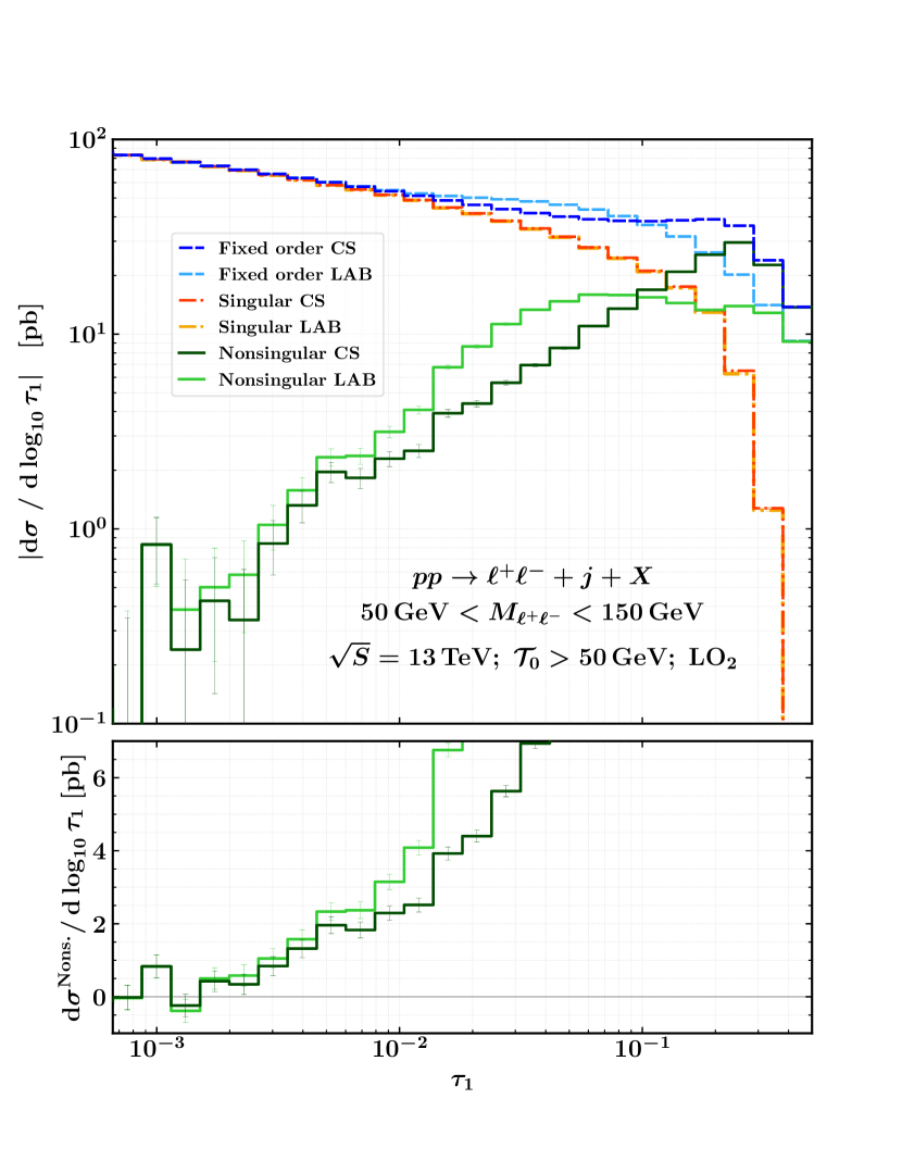
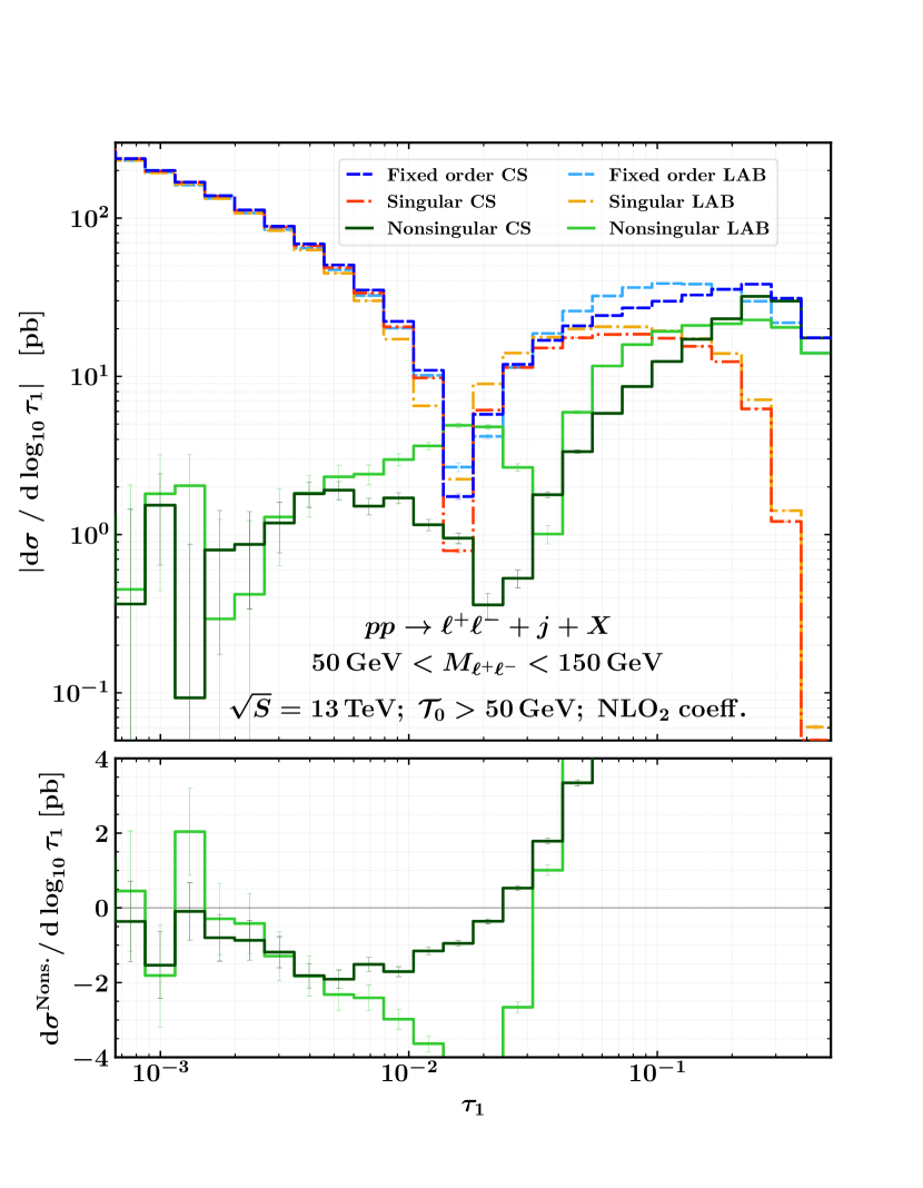
Figure 1: Absolute values of the $\tau_{1}=\mathcal{T}_{1}/m_{T}$ spectra with $\mathcal{T}_{0}>50$ GeV for fixed-order, singular and nonsingular contributions at $\mathcal{O}(\alpha_{s}^{2})$ (left) and at pure $\mathcal{O}(\alpha_{s}^{3})$ (right) on a logarithmic scale (upper frames) and signed values for the nonsingular on a linear scale (lower frames). Results for both the laboratory frame (LAB) and the frame where the colour-singlet system has zero rapidity (CS) are shown. Statistical errors from Monte Carlo integration, shown as thin vertical error bars, become sizeable at extremely low $\tau_{1}$ values.

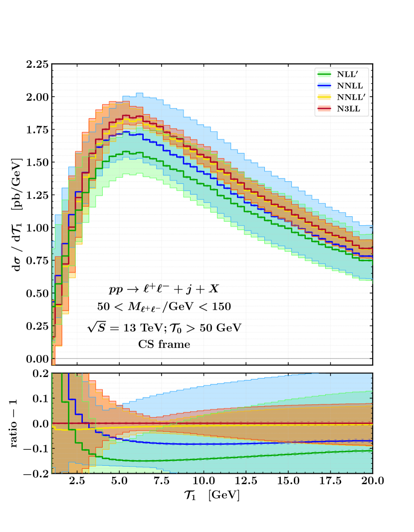
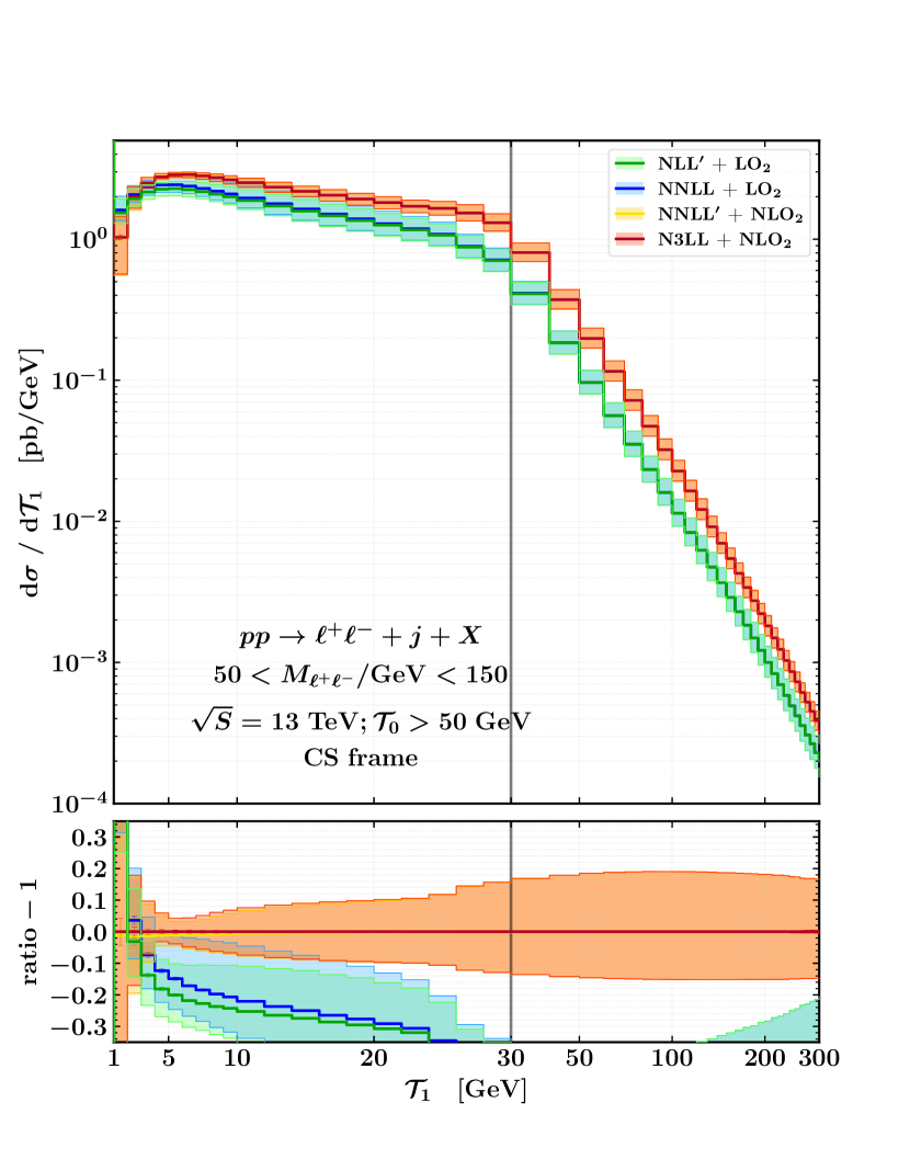
Figure 2: Resummed (left) and matched (right) results for one-jettiness distribution with $\mathcal{T}_{0}>50$ GeV.

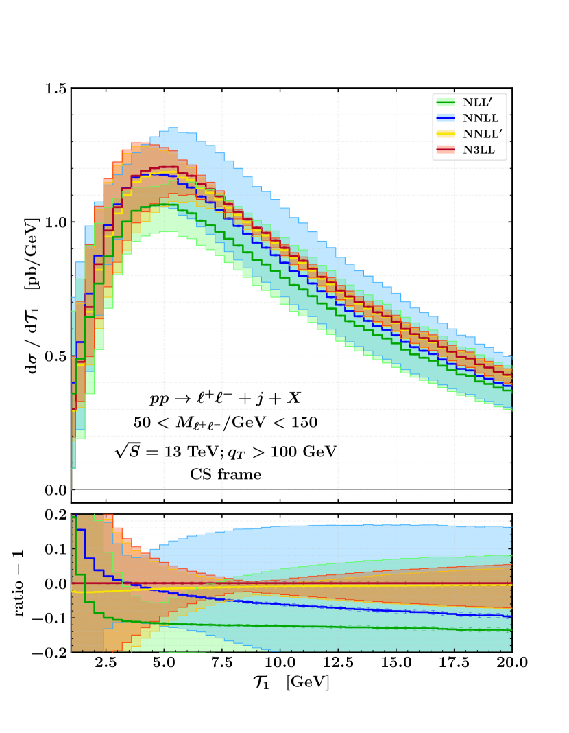
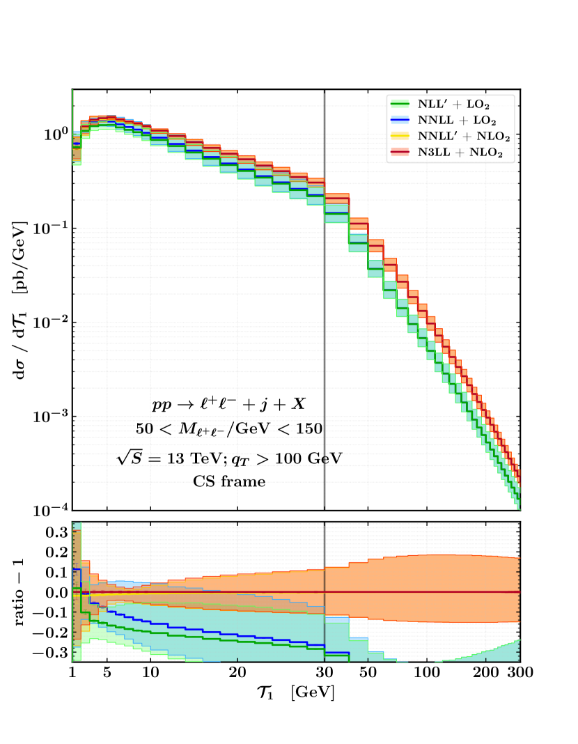
Figure 3: Resummed (left) and matched (right) results for one-jettiness distribution with $q_{T}>100$ GeV.

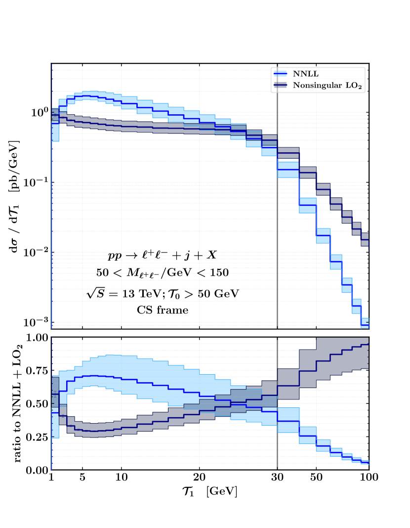
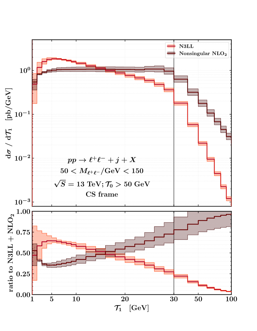
Figure 4: Comparison between resummed and nonsingular contributions at NNLL+LO₂ (left) and N³LL+NLO₂ (right) for one-jettiness distribution with $\mathcal{T}_{0}>50$ GeV. The lower inset shows the ratio to the corresponding matched prediction.

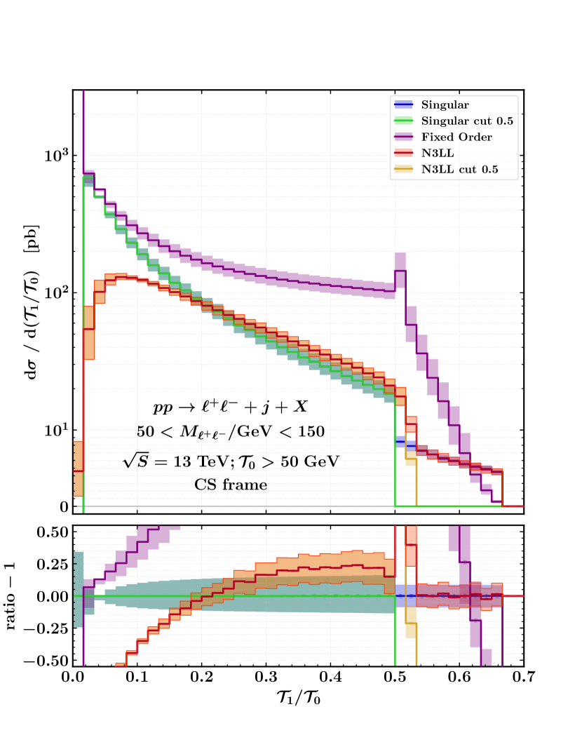
Figure 5: Comparisons between resummed N³LL results, fixed-order NLO₂ and singular ones for $\mathcal{T}_{0}>50$ GeV with or without a hard cut at $\mathcal{T}_{1}/\mathcal{T}_{0}<0.5$ on the $\mathcal{O}(\alpha_{s}^{3})$ singular contribution.

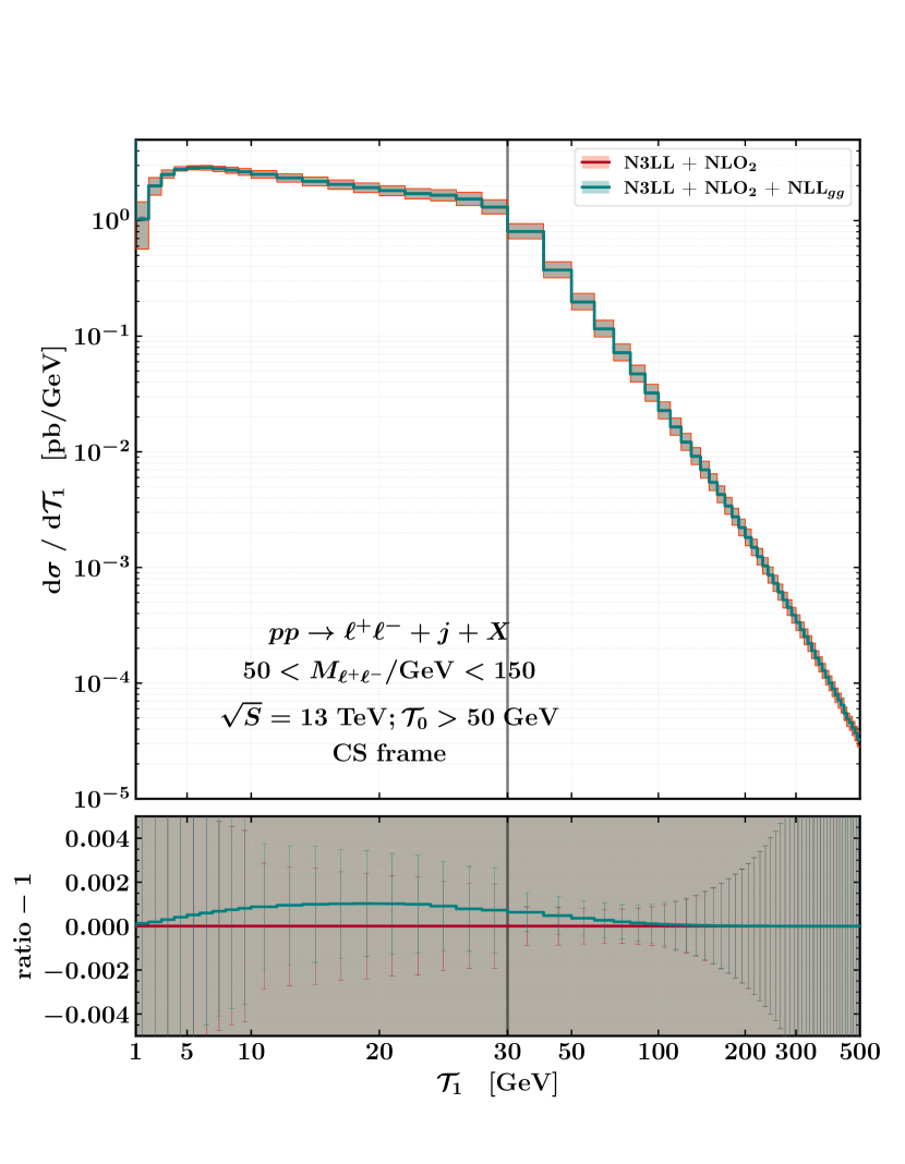
Figure 6: Effects of the inclusion of the NLL resummation of the $gg$ loop-induced channel on top of the N³LL+NLO₂ matched predictions. ——————————————————————-

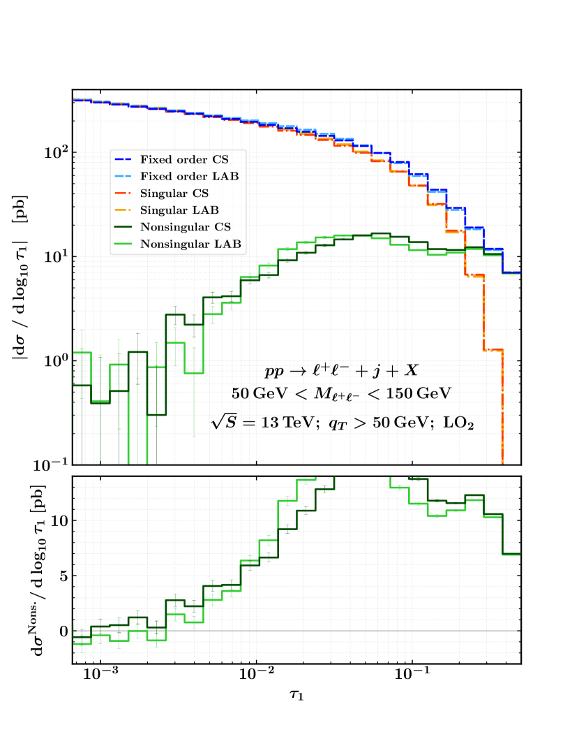
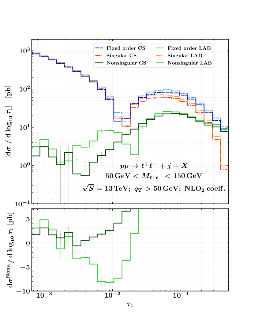
Figure 7: Absolute values of the $\tau_{1}=\mathcal{T}_{1}/m_{T}$ spectra with $q_{T}>50$ GeV for fixed-order, singular and nonsingular contributions at $\mathcal{O}(\alpha_{s}^{2})$ (left) and at pure $\mathcal{O}(\alpha_{s}^{3})$ (right) on a logarithmic scale (upper frames) and signed values for the nonsingular on a linear scale (lower frames). Results for both the laboratory frame (LAB) and the frame where the colour-singlet system has zero rapidity (CS) are shown. Statistical errors from Monte Carlo integration, shown as thin vertical error bars, become sizeable at extremely low $\tau_{1}$ values.

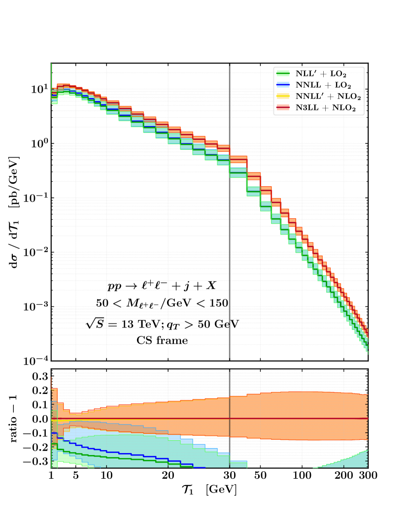
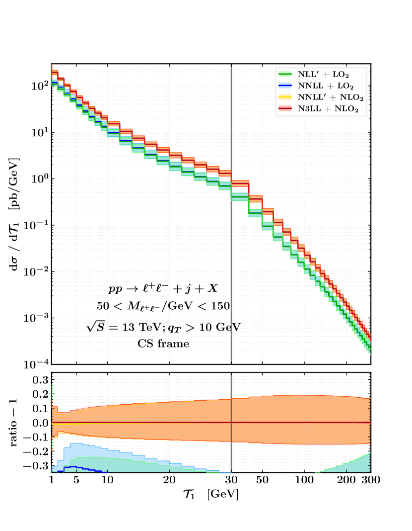
Figure 8: Resummed results matched to the appropriate fixed-order on a semilogarithmic scale with $q_{T}>50$ GeV (left) and with $q_{T}>10$ GeV (right).

We consider the process

$$pp\to(\gamma^{*}/Z\to\ell^{+}\ell^{-})+{\text{jet}}+X\,,$$

at $\sqrt{S}=13$ TeV and use the NNPDF31_nnlo_as_0118 PDF set [67].

The factorisation and renormalisation scales are set equal to each other and equal to the dilepton transverse mass,

$$\mu_{R}=\mu_{F}=\mu_{\mathrm{FO}}=m_{T}\equiv\sqrt{M^{2}_{\ell^{+}\ell^{-}}+q_{T}^{2}}\,,$$ (60)

which we also use as hard scale for the process, i.e. $\mu_{H}=\mu_{\mathrm{FO}}$. At this stage, we also fix $Q^{2}=s_{ab}$.

Here we report the numerical parameters used in the predictions, for ease of reproducibility. We set the following non-zero mass and width parameters

$$m_{\text{Z}} =91.1876\,\text{GeV}\,,\qquad \Gamma_{\text{Z}} =2.4952\,\text{GeV}\,,$$

$$m_{\text{W}} =80.379\,\text{GeV}\,,\qquad \Gamma_{\text{W}} =2.0850\,\text{GeV}\,,$$

$$m_{\text{t}} =173.1\,\text{GeV}\,.$$

In the plots presented in this section, we apply either a cut $\mathcal{T}_{0}>50$ GeV or $q_{T}>100$ GeV in order to have a well-defined Born cross section with a hard jet. However, since our predictions depend on the choice of the cut that defines a finite Born cross section, we study different variables and values to cut upon in sec. III.4.

III.1 Resummed and matched predictions

In the upper panel of Fig. 1 we show the absolute values of the spectra for fixed-order, singular and nonsingular contributions with $\mathcal{T}_{0}>50$ GeV at different orders in the strong coupling. We plot on a logarithmic scale in the dimensionless $\tau_{1}=\mathcal{T}_{1}/m_{T}$ variable, which is the argument of the logarithms appearing in the cross section for our choice of $\mu_{H}=m_{T}$. In the lower panel of the same figure we compare the nonsingular contributions in the LAB and CS frames on a linear scale. At both orders one can see how the singular spectrum reproduces the fixed-order result at small values of $\tau_{1}$ and how the nonsingular spectrum has the expected suppressed behaviour in the $\tau_{1}\to 0$ limit. As anticipated, the nonsingular contribution in the CS frame is consistently smaller than that evaluated in the laboratory frame. Due to the smaller power corrections in the nonsingular contribution, from now on we only focus on and present results in the colour-singlet frame (though the formalism adopted is able to deal with any frame definition related by a longitudinal boost). Similar results for $q_{T}$ cuts are reported in sec. III.4.

In the left panel of Fig. 2 (Fig. 3) we show our resummed predictions in the peak region of the $\mathcal{T}_{1}$ spectrum in the CS frame, with a cut $\mathcal{T}_{0}>50$ GeV ($q_{T}>100$ GeV). We observe good perturbative convergence between different orders. Starting from NNLL^′, the inclusion of NNLO boundary conditions together with NLO$\times$NLO mixed-terms in the factorisation formula results in a large impact on the central values and in a sizeable decrease of the theoretical uncertainty bands. We also notice that the differences between the N³LL and the NNLL^′ predictions are minor, suggesting that, unlike at lower-orders, the N³LL evolution does not change considerably the NNLL^′ results.

In the right panel of Fig. 2 we present our final results after additive matching to the fixed-order predictions. In order to better highlight the effects in the resummation region ($\mathcal{T}_{1}\lesssim 30$ GeV), the plot is shown on a linear $\mathcal{T}_{1}$ scale up to $30$ GeV and a logarithmic scale above. In this case, the addition of the nonsingular contributions substantially modifies the resummed predictions, both in the fixed-order ($\mathcal{T}_{1}\gtrsim 30$ GeV) but also in the resummation region. This can be better appreciated by looking at Fig. 4, which compares the values of the resummed and nonsingular predictions at NNLL+LO₂ (left panel) and at N³LL+NLO₂ (right panel). The relative size of each contribution to the corresponding matched predictions is shown in the lower inset. We note that this poor convergence is also present when cutting on the vector boson transverse momentum $q_{T}>100$ GeV in the right panel of Fig. 3 and the difference between orders grows larger when the cut is reduced (see  sec. III.4).
 
 
However, since these are the first nontrivial corrections to the $\mathcal{T}_{1}$ spectrum, their large size is not completely unexpected and further motivates their inclusion.

III.2 Two-dimensional profile scales

A final state with $N$ particles is subject to the kinematical constraint

$$\frac{\mathcal{T}_{1}(\Phi_{N})}{\mathcal{T}_{0}(\Phi_{N})}\leq\frac{N-1}{N}=\begin{cases}1/2\,,&N=2\\ 2/3\,,&N=3\end{cases}$$ (61)

where we explicitly specify the possible upper bounds that $\mathcal{T}_{1}/\mathcal{T}_{0}$ can have for the NNLO calculation of colour-singlet plus one jet. Our goal in this section is to formulate profile scales that force the resummed prediction to satisfy the phase space constraint in eq. (61) and at the same time to have the appropriate scaling at small and large $\mathcal{T}_{1}$, i.e.

$$\mu_{S}(\mathcal{T}_{1}\ll\mu_{\mathrm{FO}}) \sim\mathcal{T}_{1}\,,$$

$$\mu_{S}(\mathcal{T}_{1}\sim\mu_{\mathrm{FO}}) \sim\mu_{\mathrm{FO}}\,,$$

$$\mu_{S}\bigl{(}\mathcal{T}_{1}/\mathcal{T}_{0}\sim(N-1)/N\bigr{)} \sim\mu_{\mathrm{FO}}\,.$$ (62)

Both requirements in eqs. (61) and (62) can be satisfied by formulating two-dimensional profile scales in $\mathcal{T}_{1}/\mu_{\mathrm{FO}}$ and $\mathcal{T}_{1}/\mathcal{T}_{0}$. To this end, we choose the soft profile scale to be

$$\mu_{S}\bigl{(}\mathcal{T}_{1}/\mu_{\mathrm{FO}}, \mathcal{T}_{1}/\mathcal{T}_{0}\bigr{)}$$ (63)

$$=\mu_{\mathrm{FO}}\bigl{[}\bigl{(}f_{\rm{run}}(\mathcal{T}_{1}/\mu_{\mathrm{FO}})-1\bigr{)}s^{(p,k)}(\mathcal{T}_{1}/\mathcal{T}_{0})+1\bigr{]}$$

where $f_{\rm{run}}$ is the same as that appearing in $\mathcal{T}_{0}$ profile scales used in previous Geneva implementations, see e.g. ref. [26], while $s^{(p,k)}$ is a logistic function

$$s^{(p,k)}(\mathcal{T}_{1}/\mathcal{T}_{0})=\frac{1}{1+e^{pk(\mathcal{T}_{1}/\mathcal{T}_{0}-1/p)}}\,,$$ (64)

that behaves like a smooth theta function and controls the transition to $\mu_{\mathrm{FO}}$ for a target $\mathcal{T}_{1}/\mathcal{T}_{0}$ value. It depends on the parameters $k$ and $p$. The former fixes the slope of the transition between canonical and fixed-order scaling, while the latter determines the transition point where this happens. For our final predictions we use $p\!=\!2$ and $k\!=\!100$. In app. A we further investigate the dependence of the resummed results on the way the resummation is switched off in the $\mathcal{T}_{1}/\mathcal{T}_{0}$ direction.

Finally, it is straightforward to get the beam and jet function profile scales since they are tied to the corresponding soft profiles by

$$\mu_{B}(\mathcal{T}_{1}/\mu_{\mathrm{FO}},\mathcal{T}_{1}/\mathcal{T}_{0}\bigr{)} =\sqrt{\mu_{\mathrm{FO}}\mu_{S}(\mathcal{T}_{1}/\mu_{\mathrm{FO}},\mathcal{T}_{1}/\mathcal{T}_{0}\bigr{)}}\,,$$ (65)

$$\mu_{J}(\mathcal{T}_{1}/\mu_{\mathrm{FO}},\mathcal{T}_{1}/\mathcal{T}_{0}\bigr{)} =\sqrt{\mu_{\mathrm{FO}}\mu_{S}(\mathcal{T}_{1}/\mu_{\mathrm{FO}},\mathcal{T}_{1}/\mathcal{T}_{0}\bigr{)}}\,,$$ (66)

and for this process we set the hard scale to be

$$\mu_{H} =\mu_{\mathrm{FO}}=m_{T}\equiv\sqrt{m^{2}_{\ell^{+}\ell^{-}}+q_{T}^{2}}\,.$$ (67)

When calculating scale variations we vary $\mu_{\mathrm{FO}}$ by a factor of two in either direction. The soft, jet and beam scales variations are then calculated as detailed in ref. [26] and summed in quadrature to the hard variations.

Having discussed the implementation of the resummed predictions, some freedom remains in how to treat the $\mathcal{O}(\alpha_{s}^{3})$ singular resummed-expanded term. Since for $\mathcal{T}_{1}>\mathcal{T}_{0}/2$ only the real contribution $\mathcal{O}(\alpha_{s}^{3})$ with three particles can contribute in the fixed-order, one can decide to completely neglect both the resummed and the resummed-expanded terms above that threshold. Alternatively, one can keep them both on, but with the 2D profile scales we have chosen the resummed predictions will naturally match the singular ones for $\mathcal{T}_{1}\gtrsim\mathcal{T}_{0}/2$ and the two contributions will cancel again in the matched predictions, leaving only the fixed-order real contribution of $\mathcal{O}(\alpha_{s}^{3})$. This behaviour is shown in Fig. 6, where we plot the NLO₂ fixed-order predictions for the $\mathcal{T}_{1}/\mathcal{T}_{0}$ ratio, together with the N³LL resummed and singular ones. We include two copies of the resummed and singular predictions obtained with and without a hard cut at $\mathcal{T}_{1}/\mathcal{T}_{0}=1/2$ on the $\mathcal{O}(\alpha_{s}^{3})$ singular contribution. This is immediately evident from the fact that the singular prediction with this cut is zero above $\mathcal{T}_{1}/\mathcal{T}_{0}=1/2$. The corresponding resummed prediction does not have the same sharp jump because of the smoothing of the profile scale, but it still experiences a drastic reduction on a short $\mathcal{T}_{1}/\mathcal{T}_{0}$ range. We also notice that the singular prediction without the hard cut manifests a sudden jump: this is a consequence of the fact that for $\mathcal{T}_{1}/\mathcal{T}_{0}\leq 1/2$ both the $\mathcal{O}(\alpha_{s}^{2})$ and $\mathcal{O}(\alpha_{s}^{3})$ terms contribute, while above we only have the $\mathcal{O}(\alpha_{s}^{3})$ terms. The instability of this Sudakov shoulder region is also evident in the fixed-order predictions, showing the typical miscancellation between soft and collinear $\mathcal{O}(\alpha_{s}^{3})$ real emissions in the region $\mathcal{T}_{1}/\mathcal{T}_{0}>1/2$. These are not compensated by their virtual counterparts, which are confined to the $\mathcal{T}_{1}/\mathcal{T}_{0}\leq 1/2$ region.

For the predictions obtained in this work we have chosen to allow the singular contribution at order $\mathcal{O}(\alpha_{s}^{3})$ above $\mathcal{T}_{1}/\mathcal{T}_{0}>1/2$ up to the true kinematic limit $\mathcal{T}_{1}/\mathcal{T}_{0}=2/3$. In principle this choice affects the size of the $\mathcal{O}(\alpha_{s}^{3})$ nonsingular contribution across the whole $\mathcal{T}_{1}$ spectrum. Therefore we have carefully checked that our choice does not produce numerically significant differences with the choice of imposing $\mathcal{T}_{1}/\mathcal{T}_{0}\leq 1/2$. In fact, for the plots shown in Fig. 1 we could only spot a very minor difference in the largest bins of the $\tau_{1}$ distribution.

III.3 Effects of the inclusion of the $gg$ loop-induced channel

In this subsection we investigate the effect of the inclusion of the NLL resummation of the $gg$ loop-induced channel in addition to the N³LL+NLO₂ matched predictions. Since the $gg$ loop-induced channel starts to contribute at $\mathcal{O}(\alpha_{s}^{3})$ it is formally necessary to include it already when the resummation of the other channels is performed at NNLL^′ accuracy. However, as can be seen in Fig. 6, its contribution is extremely small across the whole $\mathcal{T}_{1}$ spectrum, reaching a maximum deviation of around one per mille between 10 and 20 GeV. The fact that this deviation is smaller than the numerical uncertainty associated with the Monte Carlo integration allows one to safely neglect this contribution.

III.4 Results with different $\mathcal{T}_{0}$ and $q_{T}$ cuts

The resummation of one-jettiness requires the presence of a hard jet to have a well-defined Born cross section. In order to investigate the effect of the selection of the hard jet here we discuss the behaviour of our preditions for different values of the $\mathcal{T}_{0}$ cut. We also present results obtained by requiring that the colour singlet has a substantial transverse momentum $q_{T}$, which is equivalent to requiring the presence of at least one hard jet with a large $k_{T}$ imbalance compared with other potential jets. Lowering the $\mathcal{T}_{0}$ cut value to 10 or 1 GeV, we observe a worsening of the convergence of the resummed predictions. Moreover, the nonsingular contribution increases with the lowering of the $\mathcal{T}_{0}$ cut value and the distance between the $\mathcal{O}(\alpha_{s}^{2})$ and $\mathcal{O}(\alpha_{s}^{3})$ contributions widens when reaching the region $\mathcal{T}_{0}\sim\mathcal{T}_{1}\ll Q$. This behaviour can be easily explained by considering that the factorisation formula in eq. (2) has been derived assuming $\mathcal{T}_{1}\ll\mathcal{T}_{0}\sim Q$. A thorough treatment of this region would necessitate a multi-differential resummation of $\mathcal{T}_{0}$ and $\mathcal{T}_{1}$, which is beyond the current state of the art [68, 69]. If we define the hard jet by placing a cut on the $q_{T}$ of the colour singlet system, we observe a similar behaviour when the cut is reduced. In Fig. 7 we show the nonsingular contributions at $\mathcal{O}(\alpha_{s}^{2})$ and $\mathcal{O}(\alpha_{s}^{3})$ with a $q_{T}>50$ GeV cut. Compared to the same plot for the $\mathcal{T}_{0}>50$ GeV cut in Fig. 1 we observe a reduced difference between the size of the power corrections for $\mathcal{T}_{1}$ definitions in the two different frames.

Finally, in Fig. 8 we show the resummed predictions matched to the fixed-order in the peak region for the additional cuts $q_{T}>50$ GeV and $q_{T}>10$ GeV. We observe that the predictions are very sensitive to the cut value, and the perturbative convergence is rapidly lost when decreasing the cut value too much.

IV Conclusions

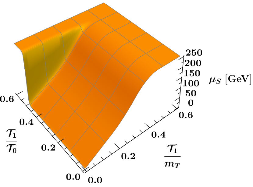
Figure 9: Functional form of the two-dimensional soft profile scale.

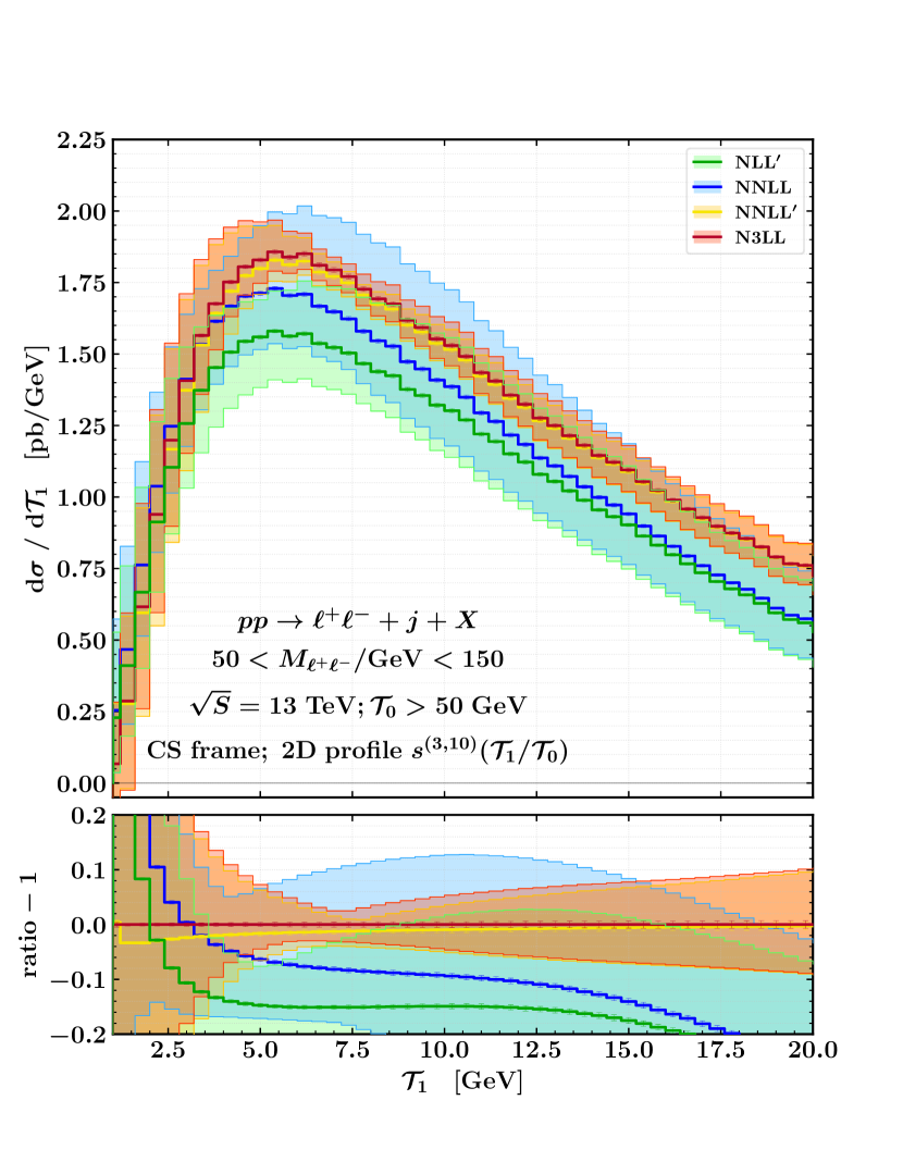
Figure 10: Resummed results for one-jettiness distribution with $\mathcal{T}_{0}>50$ GeV at increasing accuracy, for the 2D profile with $s^{(3,10)}(\mathcal{T}_{1}/\mathcal{T}_{0}).$

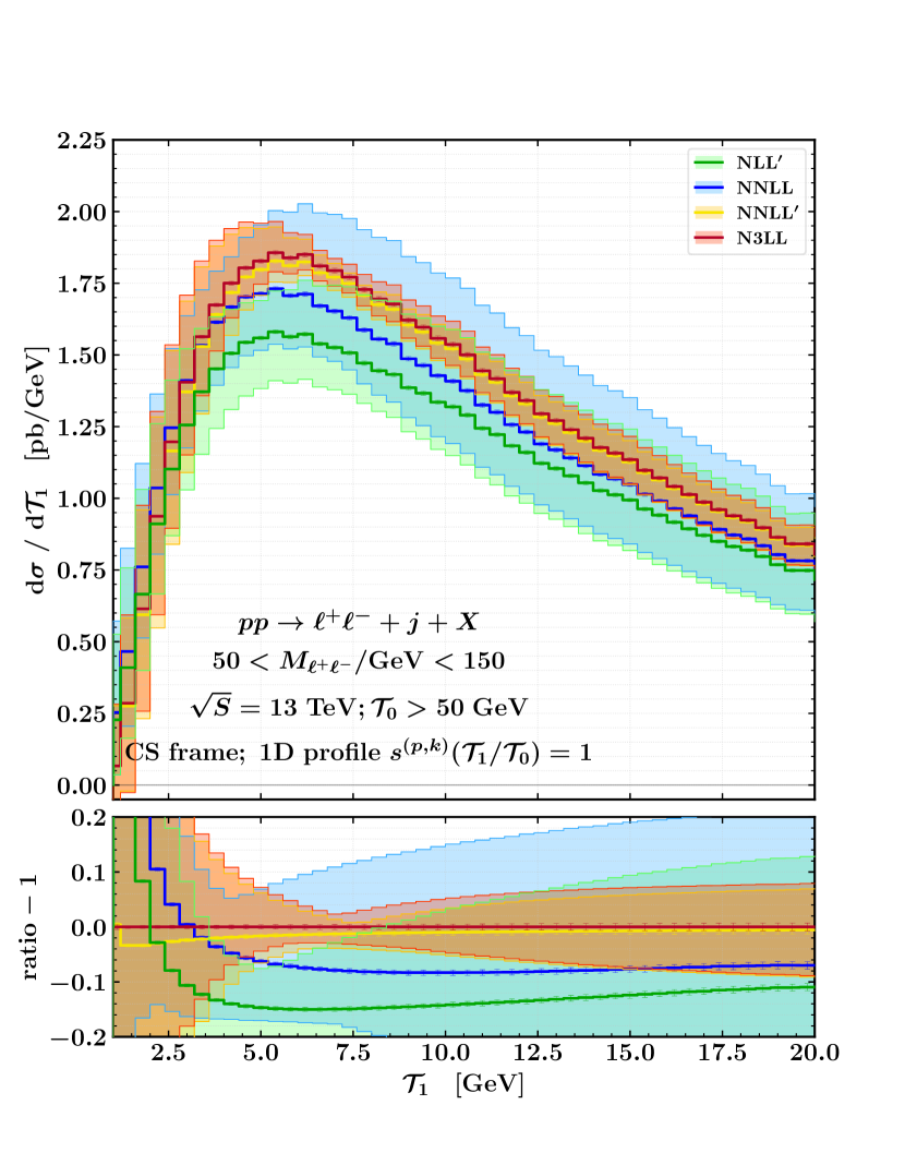
Figure 11: Resummed results for one-jettiness distribution with $\mathcal{T}_{0}>50$ GeV at increasing accuracy, for the 1D flat profile $s^{(p,k)}(\mathcal{T}_{1}/\mathcal{T}_{0})=1$.

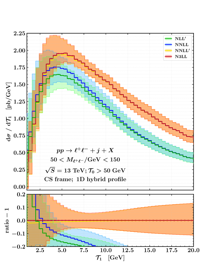
Figure 12: Resummed results for one-jettiness distribution with $\mathcal{T}_{0}>50$ GeV at increasing accuracy, for the 1D hybrid profile discussed in the text.

In this work, we presented novel predictions for the $\mathcal{T}_{1}$ spectrum of the process $pp\to(\gamma^{*}/Z\to\ell^{+}\ell^{-})+{\text{jet}}$ at NNLL^′ and N³LL accuracy in resummed perturbation theory. By matching these results to the appropriate fixed-order calculation, we obtained an accurate description of the spectrum across the entire kinematic range. This is the first time that results at this accuracy have been presented for a process with three coloured partons at Born level. Our calculation includes all two-loop singular terms as $\mathcal{T}_{1}\to 0$, off-shell effects of the vector bosons, the $Z/\gamma^{*}$ interference, as well as spin correlations.

The resummed predictions in the colour-singlet frame exhibit a good perturbative convergence, with a significant reduction of theoretical uncertainties as the perturbative order is increased. Notably, the inclusion of N³LL evolution has only a minor effect on our final results. The matching to the fixed-order calculation was achieved by switching off the resummation in the hard region of phase space by means of two-dimensional profile scales, which allow for the kinematic restrictions on the one-jettiness variable to be enforced consistently. Our matched results indicate that the inclusion of the $\mathcal{O}(\alpha_{s}^{3})$ nonsingular terms is important due to their large size.

In order to assess the consistency of our implementation, we checked the explicit cancellation of the arbitrary $\mu$ dependence which appears in the separate evolution of each of the ingredients in the factorisation formula and that the singular structure of the resummed expanded results matches that of the relative fixed order. We found that, in accordance with observations in the literature, the definition of $\mathcal{T}_{1}$ in the laboratory frame is subject to larger nonsingular contributions. These arise due to the dependence of the observable on the longitudinal boost between the hadronic and the partonic centre-of-mass frames. To mitigate their impact, we found that a different definition of $\mathcal{T}_{1}$ (which incorporates a longitudinal boost to the frame where the vector boson has zero rapidity) receives smaller power corrections. This makes it suitable for slicing calculations at NNLO and for use in Monte Carlo event generators which match fixed order predictions to parton shower programs.

The $N$-jettiness variable is particularly useful in the context of constructing higher-order event generators, since it is able to act as a resolution variable which divides the phase space into exclusive jet bins. In this context, the NNLL^′ resummed zero-jettiness spectrum has enabled the construction of NNLO+PS generators for colour-singlet production using the Geneva method. The availability of an equally accurate prediction for $\mathcal{T}_{1}$ in hadronic collisions will now enable these generators to be extended to cover the case of colour singlet production in association with a jet. The predictions presented in this work will be made public in a future release of Geneva.
 
Acknowledgements. We are grateful to our Geneva collaborators (A. Gavardi and S. Kallweit) for their work on the code. We would also like to thank T. Becher for discussions about the colour structures of the hard anomalous dimension and F. Tackmann for carefully reading the manuscript and for useful comments and suggestions in the presentation of the results.

The work of SA, AB, RN and DN has been partially supported by the ERC Starting Grant REINVENT-714788. The work of SA and GBi is also supported by MIUR through the FARE grant R18ZRBEAFC. MAL is supported by the UKRI guarantee scheme for the Marie Skłodowska-Curie postdoctoral fellowship, grant ref. EP/X021416/1. The work of D.N. is supported by the European Union - Next Generation EU (H45E22001270006). The work of GBe was supported by the Deutsche Forschungsgemeinschaft (DFG, German Research Foundation) under grant 396021762 - TRR 257. RR is supported by the Royal Society through Grant URF\R1\201500. GM and BD have received funding from the European Research Council (ERC) under the European Union’s Horizon 2020 research and innovation programme (Grant agreement No. 101002090 COLORFREE). GM also acknowledges support from the Deutsche Forschungsgemeinschaft (DFG) under Germany’s Excellence Strategy – EXC 2121 “Quantum Universe”– 390833306 and BD from the Helmholtz Association Grant W2/W3-116.

We acknowledge financial support, supercomputing resources and support from ICSC – Centro Nazionale di Ricerca in High Performance Computing, Big Data and Quantum Computing – and hosting entity, funded by European Union – NextGenerationEU.

Appendix A Alternative profile scale choices

In this appendix we study the dependence of the resummed results on the profile scale definition in the $(\mathcal{T}_{1}/m_{T},\mathcal{T}_{1}/\mathcal{T}_{0})$ plane. We start by showing the functional form of $\mu_{S}$ for the default 2D profile scales in Fig. 10. As observed, when the LO₂ kinematical constraint eq. (61) is satisfied, the factor $s^{(2,100)}(\mathcal{T}_{1}/\mathcal{T}_{0}\lesssim 1/2)\to 1$ in eq. (63) and therefore the scaling of $\mu_{S}$ is entirely dictated by $f_{\rm{run}}$, depending only on the value of $\mathcal{T}_{1}/\mu_{\mathrm{FO}}$. On the other hand, when the $\mathcal{T}_{1}/\mathcal{T}_{0}\leq 1/2$ condition is violated, $s^{(2,100)}(\mathcal{T}_{1}/\mathcal{T}_{0}\gtrsim 1/2)\to 0$, which implies that $\mu_{S}=\mu_{\mathrm{FO}}$. This is a crucial asymptotic limit, since for $\mathcal{T}_{1}/\mathcal{T}_{0}\gtrsim 1/2$ the fixed-order and singular cross sections pass a kinematical boundary. Therefore, since the fixed-order corrections are extremely relevant in that region, care must be taken to switch off the $\mathcal{T}_{1}$ resummation before passing the same threshold.

In Fig. 10 we show resummed predictions obtained using 2D profiles with $p\!=\!3$ and $k\!=\!10$, which results in a earlier and smoother switch-off of the resummation around $\mathcal{T}_{1}/\mathcal{T}_{0}\sim 1/3$. As one can see by comparing the results with the left panel of Fig. 2, by doing so the convergence of successive perturbative orders is slightly worsened. Alternatively, we have explored the usage of 1D profile scales, either by removing the suppression in the $\mathcal{T}_{1}/\mathcal{T}_{0}$ direction, see Fig. 12, or by switching off the resummation in the $\mathcal{T}_{1}/\mathcal{T}_{0}$ direction by means of a 1D hybrid profile, see Fig. 12. The hybrid profile approach has previously been successfully used in enforcing multi-differential profile scales switch-offs [70]. In our case it is defined by

$$\mu_{S}\bigl{(}\mathcal{T}_{1}/\mu_{\mathrm{FO}}, \mathcal{T}_{1}/\mathcal{T}_{0}\bigr{)}$$ (68)

$$=\mu_{\mathrm{FO}}f_{\rm{run}}(\mathcal{T}_{1}/\mathcal{T}_{0})+\mathcal{T}_{1}\bigl{(}1-f_{\rm{run}}(\mathcal{T}_{1}/\mathcal{T}_{0})\bigr{)}\,,$$

where now the argument of $f_{\rm{run}}$ is the ratio $\mathcal{T}_{1}/\mathcal{T}_{0}$ rather than $\mathcal{T}_{1}/\mu_{\mathrm{FO}}$. The formula in eq. (68) smoothly interpolates between $\mathcal{T}_{1}$ and $\mu_{\mathrm{FO}}$ on a diagonal slice of the $(\mathcal{T}_{1}/\mathcal{T}_{0},\mathcal{T}_{1}/m_{T})$ plane. In Fig. 12 we observe that removing the $\mathcal{T}_{1}/\mathcal{T}_{0}$ suppression has very small effects on the $\mathcal{T}_{1}$ distribution, maintaining a good perturbative convergence across orders. This, however, does not provide the correct suppression of the resummation effects past the kinematic endpoint in the $\mathcal{T}_{1}/\mathcal{T}_{0}$ direction. The usage of the hybrid profile shows instead a much poorer convergence (see Fig. 12). In particular, we notice a change in the resummed predictions also in the peak region, which should follow a canonical scaling. This is easily explained by the fact that for the hybrid profiles in eq. (68) the $\mu_{S}$ behaviour at low $\mathcal{T}_{1}$ is changed from $\mathcal{T}_{1}$ to $(1+m_{T}/\mathcal{T}_{0})\mathcal{T}_{1}$, which is still a canonical scaling but includes small artificial leftover logarithms.

Appendix B Resummed formula at N³LL accuracy

In this section we report the full formula for the N³LL resummation with the explicit combination of the hard, soft, beam and jet boundary terms, evaluated at the appropriate order, for completeness. It reads

$$\frac{\mathrm{d}\sigma^{\textsc{n}^{3}\textsc{ll}}}{\mathrm{d}\Phi_{1}\mathrm{d}\mathcal{T}_{1}}= \sum_{\kappa}\exp\bigg{\{}4(C_{a}+C_{b})K^{\textsc{n}^{3}\textsc{ll}}_{\Gamma_{\mathrm{cusp}}}(\mu_{B},\mu_{H})+4C_{c}K^{\textsc{n}^{3}\textsc{ll}}_{\Gamma_{\mathrm{cusp}}}(\mu_{J},\mu_{H})-2(C_{a}+C_{b}+C_{c})K^{\textsc{n}^{3}\textsc{ll}}_{\Gamma_{\mathrm{cusp}}}(\mu_{S},\mu_{H})$$

$$\quad\qquad\quad-2C_{c}L_{J}\ \eta^{\textsc{n}^{3}\textsc{ll}}_{\Gamma_{\mathrm{cusp}}}(\mu_{J},\mu_{H})-2(C_{a}L_{B}+C_{b}L^{\prime}_{B})\eta^{\textsc{n}^{3}\textsc{ll}}_{\Gamma_{\mathrm{cusp}}}(\mu_{B},\mu_{H})+K^{\textsc{n}^{3}\textsc{ll}}_{\gamma_{\rm tot}}$$

$$\quad+\bigg{[}C_{a}\ln\left(\frac{Q^{2}_{a}u}{st}\right)+C_{b}\ln\left(\frac{Q^{2}_{b}t}{su}\right)+C_{\kappa_{j}}\ln\left(\frac{Q^{2}_{J}s}{tu}\right)+(C_{a}+C_{b}+C_{c})L_{S}\bigg{]}\eta^{\textsc{n}^{3}\textsc{ll}}_{\Gamma_{\mathrm{cusp}}}(\mu_{S},\mu_{H})$$

$$+\sum_{R=F,A}\bigg{[}8\,\big{(}D_{aR}+D_{bR}\big{)}K^{\textsc{n}^{3}\textsc{ll}}_{g^{R}}(\mu_{B},\mu_{H})+8\,D_{cR}K^{\textsc{n}^{3}\textsc{ll}}_{g^{R}}(\mu_{J},\mu_{H})\,$$

$$\qquad-4\,\big{(}D_{aR}+D_{bR}+D_{cR}\big{)}K^{\textsc{n}^{3}\textsc{ll}}_{g^{R}}(\mu_{S},\mu_{H})\,-4D_{cR}L_{J}\eta^{\textsc{n}^{3}\textsc{ll}}_{g^{R}}(\mu_{J},\mu_{H})\,-4\,\big{(}D_{aR}L_{B}+D_{bR}L^{\prime}_{B}\big{)}\eta^{\textsc{n}^{3}\textsc{ll}}_{g^{R}}(\mu_{B},\mu_{H})$$

$$\qquad+2\,\bigg{[}D_{aR}\ln\bigg{(}\frac{Q^{2}_{a}u}{st}\bigg{)}+D_{bR}\ln\bigg{(}\frac{Q^{2}_{b}t}{su}\bigg{)}+D_{cR}\ln\bigg{(}\frac{Q^{2}_{J}s}{tu}\bigg{)}\,+\big{(}D_{aR}+D_{bR}+D_{cR}\big{)}L_{S}\bigg{]}\eta^{\textsc{n}^{3}\textsc{ll}}_{g^{R}}(\mu_{S},\mu_{H})\bigg{]}\bigg{\}}$$

$$\times\bigg{\{}H^{(0)}_{\kappa}(\Phi_{1},\mu_{H})\bigg{[}f_{\kappa_{a}}(x_{a},\mu_{B})f_{\kappa_{b}}(x_{b},\mu_{B})\bigg{(}1+\frac{\alpha_{s}(\mu_{S})}{4\pi}\tilde{S}^{\kappa\,(1)}\left(\partial_{\eta_{S}}+L_{S},\mu_{S}\right)$$

$$\qquad+\frac{\alpha_{s}(\mu_{J})}{4\pi}\tilde{J}^{(1)}_{\kappa_{J}}(\partial_{\eta_{J}}+L_{J},\mu_{J})+\frac{\alpha_{s}(\mu_{S})\alpha_{s}(\mu_{J})}{16\pi^{2}}\tilde{J}^{(1)}_{\kappa_{J}}(\partial_{\eta_{J}}+L_{J},\mu_{J})\tilde{S}^{\kappa\,(1)}\left(\partial_{\eta_{S}}+L_{S},\mu_{S}\right)$$

$$\qquad+\frac{\alpha_{s}^{2}(\mu_{S})}{16\pi^{2}}\tilde{S}^{\kappa\,(2)}\left(\partial_{\eta_{S}}+L_{S},\mu_{S}\right)+\frac{\alpha_{s}^{2}(\mu_{J})}{16\pi^{2}}\tilde{J}^{(2)}_{\kappa_{J}}(\partial_{\eta_{J}}+L_{J},\mu_{J})\bigg{)}$$

$$\qquad+\bigg{(}\frac{\alpha_{s}(\mu_{B})}{4\pi}\tilde{B}^{(1)}_{\kappa_{a}}(\partial_{\eta_{B}}+L_{B},x_{a},\mu_{B})\Big{(}1+\frac{\alpha_{s}(\mu_{S})}{4\pi}\tilde{S}^{\kappa\,(1)}\left(\partial_{\eta_{S}}+L_{S},\mu_{S}\right)$$

$$\qquad+\frac{\alpha_{s}(\mu_{J})}{4\pi}\tilde{J}^{(1)}_{\kappa_{J}}(\partial_{\eta_{J}}+L_{J},\mu_{J})\Big{)}+\frac{\alpha_{s}^{2}(\mu_{B})}{16\pi^{2}}\tilde{B}^{(2)}_{\kappa_{a}}(\partial_{\eta_{B}}+L_{B},x_{a},\mu_{B})\bigg{)}f_{\kappa_{b}}(x_{b},\mu_{B})$$

$$\qquad+f_{\kappa_{a}}(x_{a},\mu_{B})\bigg{(}\frac{\alpha_{s}^{2}(\mu_{B})}{16\pi^{2}}\tilde{B}^{(2)}_{\kappa_{b}}(\partial_{\eta_{B}^{\prime}}+L_{B}^{\prime},x_{b},\mu_{B})+\frac{\alpha_{s}(\mu_{B})}{4\pi}\tilde{B}^{(1)}_{\kappa_{b}}(\partial_{\eta_{B}^{\prime}}+L_{B}^{\prime},x_{b},\mu_{B})\times$$

$$\qquad\quad\Big{(}1+\frac{\alpha_{s}(\mu_{S})}{4\pi}\tilde{S}^{\kappa\,(1)}\left(\partial_{\eta_{S}}+L_{S},\mu_{S}\right)+\frac{\alpha_{s}(\mu_{J})}{4\pi}\tilde{J}^{(1)}_{\kappa_{J}}(\partial_{\eta_{J}}+L_{J},\mu_{J})\Big{)}\bigg{)}\bigg{]}$$

$$\quad+\frac{\alpha_{s}(\mu_{H})}{4\pi}H^{(1)}_{\kappa}(\Phi_{1},\mu_{H})\bigg{[}f_{\kappa_{a}}(x_{a},\mu_{B})f_{\kappa_{b}}(x_{b},\mu_{B})\bigg{(}1+\frac{\alpha_{s}(\mu_{S})}{4\pi}\tilde{S}^{\kappa\,(1)}\left(\partial_{\eta_{S}}+L_{S},\mu_{S}\right)$$

$$\qquad+\frac{\alpha_{s}(\mu_{J})}{4\pi}\tilde{J}^{(1)}_{\kappa_{J}}(\partial_{\eta_{J}}+L_{J},\mu_{J})\bigg{)}+\bigg{(}\frac{\alpha_{s}(\mu_{B})}{4\pi}\tilde{B}^{(1)}_{\kappa_{a}}(\partial_{\eta_{B}}+L_{B},x_{a},\mu_{B})f_{\kappa_{b}}(x_{b},\mu_{B})$$

$$\quad+\frac{\alpha_{s}(\mu_{B})}{4\pi}f_{\kappa_{a}}(x_{a},\mu_{B})\tilde{B}^{(1)}_{\kappa_{b}}(\partial_{\eta_{B}^{\prime}}+L_{B}^{\prime},x_{b},\mu_{B})\bigg{)}\bigg{]}$$

$$\quad+\frac{\alpha_{s}^{2}(\mu_{H})}{16\pi^{2}}H^{(2)}_{\kappa}(\Phi_{1},\mu_{H})f_{\kappa_{a}}(x_{a},\mu_{B})f_{\kappa_{b}}(x_{b},\mu_{B})\bigg{\}}\times\frac{Q^{-\eta^{{\textsc{n}^{3}\textsc{ll}}}_{\rm tot}}}{{\mathcal{T}_{1}}^{1-\eta^{{\textsc{n}^{3}\textsc{ll}}}_{\rm tot}}}\,\frac{\eta^{{\textsc{n}^{3}\textsc{ll}}}_{\rm tot}\ e^{-\gamma_{E}\eta^{{\textsc{n}^{3}\textsc{ll}}}_{\rm tot}}}{\Gamma(1+\eta^{{\textsc{n}^{3}\textsc{ll}}}_{\rm tot})}\,.$$ (69)

References

- Gehrmann-De Ridder et al. [2016a] A. Gehrmann-De Ridder, T. Gehrmann, E. W. N. Glover, A. Huss, and T. A. Morgan, Phys. Rev. Lett. 117, 022001 (2016a), arXiv:1507.02850 [hep-ph] .
- Gehrmann-De Ridder et al. [2016b] A. Gehrmann-De Ridder, T. Gehrmann, E. W. N. Glover, A. Huss, and T. A. Morgan, JHEP 07, 133, arXiv:1605.04295 [hep-ph] .
- Gehrmann-De Ridder et al. [2016c] A. Gehrmann-De Ridder, T. Gehrmann, E. W. N. Glover, A. Huss, and T. A. Morgan, JHEP 11, 094, [Erratum: JHEP 10, 126 (2018)], arXiv:1610.01843 [hep-ph] .
- Gehrmann-De Ridder et al. [2018] A. Gehrmann-De Ridder, T. Gehrmann, E. W. N. Glover, A. Huss, and D. M. Walker, Phys. Rev. Lett. 120, 122001 (2018), arXiv:1712.07543 [hep-ph] .
- Gehrmann-De Ridder et al. [2019] A. Gehrmann-De Ridder, T. Gehrmann, E. W. N. Glover, A. Huss, and D. M. Walker, Eur. Phys. J. C 79, 526 (2019), arXiv:1901.11041 [hep-ph] .
- Gauld et al. [2020] R. Gauld, A. Gehrmann-De Ridder, E. W. N. Glover, A. Huss, and I. Majer, Phys. Rev. Lett. 125, 222002 (2020), arXiv:2005.03016 [hep-ph] .
- Bizoń et al. [2018] W. Bizoń, X. Chen, A. Gehrmann-De Ridder, T. Gehrmann, N. Glover, A. Huss, P. F. Monni, E. Re, L. Rottoli, and P. Torrielli, JHEP 12, 132, arXiv:1805.05916 [hep-ph] .
- Bizon et al. [2019] W. Bizon, A. Gehrmann-De Ridder, T. Gehrmann, N. Glover, A. Huss, P. F. Monni, E. Re, L. Rottoli, and D. M. Walker, Eur. Phys. J. C 79, 868 (2019), arXiv:1905.05171 [hep-ph] .
- Re et al. [2021] E. Re, L. Rottoli, and P. Torrielli 10.1007/JHEP09(2021)108 (2021), arXiv:2104.07509 [hep-ph] .
- Camarda et al. [2021] S. Camarda, L. Cieri, and G. Ferrera, Phys. Rev. D 104, L111503 (2021), arXiv:2103.04974 [hep-ph] .
- Chen et al. [2022] X. Chen, T. Gehrmann, E. W. N. Glover, A. Huss, P. F. Monni, E. Re, L. Rottoli, and P. Torrielli, Phys. Rev. Lett. 128, 252001 (2022), arXiv:2203.01565 [hep-ph] .
- Neumann and Campbell [2023] T. Neumann and J. Campbell, Phys. Rev. D 107, L011506 (2023), arXiv:2207.07056 [hep-ph] .
- Camarda et al. [2023] S. Camarda, L. Cieri, and G. Ferrera, Phys. Lett. B 845, 138125 (2023), arXiv:2303.12781 [hep-ph] .
- Billis et al. [2023] G. Billis, M. A. Ebert, J. K. L. Michel, and F. J. Tackmann, DESY-23-081, MIT-CTP 5572 (2023).
- Aad et al. [2023] G. Aad et al. (ATLAS), (2023), arXiv:2309.12986 [hep-ex] .
- Stewart et al. [2011] I. W. Stewart, F. J. Tackmann, and W. J. Waalewijn, Phys. Rev. Lett. 106, 032001 (2011), arXiv:1005.4060 [hep-ph] .
- Gaunt et al. [2015] J. Gaunt, M. Stahlhofen, F. J. Tackmann, and J. R. Walsh, (2015), arXiv:1505.04794 [hep-ph] .
- Boughezal et al. [2015a] R. Boughezal, C. Focke, X. Liu, and F. Petriello, (2015a), arXiv:1504.02131 [hep-ph] .
- Boughezal et al. [2016] R. Boughezal, J. M. Campbell, R. K. Ellis, C. Focke, W. T. Giele, X. Liu, and F. Petriello, Phys. Rev. Lett. 116, 152001 (2016), arXiv:1512.01291 [hep-ph] .
- Boughezal et al. [2015b] R. Boughezal, C. Focke, W. Giele, X. Liu, and F. Petriello, Phys. Lett. B 748, 5 (2015b), arXiv:1505.03893 [hep-ph] .
- Campbell et al. [2019] J. M. Campbell, R. K. Ellis, and S. Seth, JHEP 10, 136, arXiv:1906.01020 [hep-ph] .
- Alioli et al. [2015] S. Alioli, C. W. Bauer, C. Berggren, F. J. Tackmann, and J. R. Walsh, Phys. Rev. D92, 094020 (2015), arXiv:1508.01475 [hep-ph] .
- Alioli et al. [2020] S. Alioli, A. Broggio, A. Gavardi, S. Kallweit, M. A. Lim, R. Nagar, D. Napoletano, and L. Rottoli, (2020), arXiv:2009.13533 [hep-ph] .
- Jouttenus et al. [2013] T. T. Jouttenus, I. W. Stewart, F. J. Tackmann, and W. J. Waalewijn, Phys. Rev. D 88, 054031 (2013), arXiv:1302.0846 [hep-ph] .
- Alioli et al. [2022] S. Alioli, A. Broggio, and M. A. Lim, JHEP 01, 066, arXiv:2111.03632 [hep-ph] .
- Alioli et al. [2019] S. Alioli, A. Broggio, S. Kallweit, M. A. Lim, and L. Rottoli, Phys. Rev. D 100, 096016 (2019), arXiv:1909.02026 [hep-ph] .
- Alioli et al. [2021a] S. Alioli, A. Broggio, A. Gavardi, S. Kallweit, M. A. Lim, R. Nagar, D. Napoletano, and L. Rottoli, JHEP 04, 041, arXiv:2010.10498 [hep-ph] .
- Alioli et al. [2021b] S. Alioli, A. Broggio, A. Gavardi, S. Kallweit, M. A. Lim, R. Nagar, and D. Napoletano, Phys. Lett. B 818, 136380 (2021b), arXiv:2103.01214 [hep-ph] .
- Alioli et al. [2023a] S. Alioli, G. Billis, A. Broggio, A. Gavardi, S. Kallweit, M. A. Lim, G. Marinelli, R. Nagar, and D. Napoletano, JHEP 06, 205, arXiv:2212.10489 [hep-ph] .
- Alioli et al. [2023b] S. Alioli, G. Billis, A. Broggio, A. Gavardi, S. Kallweit, M. A. Lim, G. Marinelli, R. Nagar, and D. Napoletano, JHEP 05, 128, arXiv:2301.11875 [hep-ph] .
- Becher and Neubert [2020] T. Becher and M. Neubert, JHEP 01, 025, arXiv:1908.11379 [hep-ph] .
- Henn et al. [2020] J. M. Henn, G. P. Korchemsky, and B. Mistlberger, JHEP 04, 018, arXiv:1911.10174 [hep-th] .
- von Manteuffel et al. [2020] A. von Manteuffel, E. Panzer, and R. M. Schabinger, Phys. Rev. Lett. 124, 162001 (2020), arXiv:2002.04617 [hep-ph] .
- Boughezal et al. [2015c] R. Boughezal, X. Liu, and F. Petriello, Phys. Rev. D 91, 094035 (2015c), arXiv:1504.02540 [hep-ph] .
- Campbell et al. [2018] J. M. Campbell, R. K. Ellis, R. Mondini, and C. Williams, Eur. Phys. J. C 78, 234 (2018), arXiv:1711.09984 [hep-ph] .
- Bell et al. [pear] G. Bell, B. Dehnadi, T. Mohrmann, and R. Rahn, (to appear).
- Stewart et al. [2010a] I. W. Stewart, F. J. Tackmann, and W. J. Waalewijn, Phys. Rev. D 81, 094035 (2010a), arXiv:0910.0467 [hep-ph] .
- Stewart et al. [2010b] I. W. Stewart, F. J. Tackmann, and W. J. Waalewijn, Phys. Rev. Lett. 105, 092002 (2010b), arXiv:1004.2489 [hep-ph] .
- Sjödahl [2013] M. Sjödahl, Eur. Phys. J. C 73, 2310 (2013), arXiv:1211.2099 [hep-ph] .
- Liu and Stahlhofen [2021] Z. L. Liu and M. Stahlhofen, JHEP 02, 128, arXiv:2010.05861 [hep-ph] .
- Garland et al. [2002] L. W. Garland, T. Gehrmann, E. W. N. Glover, A. Koukoutsakis, and E. Remiddi, Nucl. Phys. B 642, 227 (2002), arXiv:hep-ph/0206067 .
- Gehrmann and Tancredi [2012] T. Gehrmann and L. Tancredi, JHEP 02, 004, arXiv:1112.1531 [hep-ph] .
- Becher et al. [2014] T. Becher, G. Bell, C. Lorentzen, and S. Marti, JHEP 02, 004, arXiv:1309.3245 [hep-ph] .
- Campbell and Ellis [2017] J. M. Campbell and R. K. Ellis, JHEP 01, 020, arXiv:1610.02189 [hep-ph] .
- Gehrmann et al. [2023] T. Gehrmann, T. Peraro, and L. Tancredi, JHEP 02, 041, arXiv:2211.13596 [hep-ph] .
- Stewart et al. [2010c] I. W. Stewart, F. J. Tackmann, and W. J. Waalewijn, JHEP 1009, 005, arXiv:1002.2213 [hep-ph] .
- Ligeti et al. [2008] Z. Ligeti, I. W. Stewart, and F. J. Tackmann, Phys. Rev. D 78, 114014 (2008), arXiv:0807.1926 [hep-ph] .
- Gaunt et al. [2014a] J. R. Gaunt, M. Stahlhofen, and F. J. Tackmann, JHEP 04, 113, arXiv:1401.5478 [hep-ph] .
- Gaunt et al. [2014b] J. Gaunt, M. Stahlhofen, and F. J. Tackmann, JHEP 08, 020, arXiv:1405.1044 [hep-ph] .
- Ebert et al. [2020] M. A. Ebert, B. Mistlberger, and G. Vita, JHEP 09, 143, arXiv:2006.03056 [hep-ph] .
- Baranowski et al. [2023] D. Baranowski, A. Behring, K. Melnikov, L. Tancredi, and C. Wever, JHEP 02, 073, arXiv:2211.05722 [hep-ph] .
- Bauer and Manohar [2004] C. W. Bauer and A. V. Manohar, Phys. Rev. D 70, 034024 (2004), arXiv:hep-ph/0312109 .
- Bosch et al. [2004] S. W. Bosch, B. O. Lange, M. Neubert, and G. Paz, Nucl. Phys. B 699, 335 (2004), arXiv:hep-ph/0402094 .
- Becher and Neubert [2006] T. Becher and M. Neubert, Phys. Lett. B637, 251 (2006), hep-ph/0603140 .
- Becher and Schwartz [2010] T. Becher and M. D. Schwartz, JHEP 02, 040, arXiv:0911.0681 [hep-ph] .
- Becher and Bell [2011] T. Becher and G. Bell, Phys. Lett. B 695, 252 (2011), arXiv:1008.1936 [hep-ph] .
- Brüser et al. [2018] R. Brüser, Z. L. Liu, and M. Stahlhofen, Phys. Rev. Lett. 121, 072003 (2018), arXiv:1804.09722 [hep-ph] .
- Banerjee et al. [2018] P. Banerjee, P. K. Dhani, and V. Ravindran, Phys. Rev. D 98, 094016 (2018), arXiv:1805.02637 [hep-ph] .
- Jouttenus et al. [2011] T. T. Jouttenus, I. W. Stewart, F. J. Tackmann, and W. J. Waalewijn, Phys. Rev. D 83, 114030 (2011), arXiv:1102.4344 [hep-ph] .
- Billis et al. [2021] G. Billis, M. A. Ebert, J. K. L. Michel, and F. J. Tackmann, Eur. Phys. J. Plus 136, 214 (2021), arXiv:1909.00811 [hep-ph] .
- Bell et al. [2018] G. Bell, R. Rahn, and J. Talbert, Nucl. Phys. B 936, 520 (2018), arXiv:1805.12414 [hep-ph] .
- Bell et al. [2019] G. Bell, R. Rahn, and J. Talbert, JHEP 07, 101, arXiv:1812.08690 [hep-ph] .
- Bell et al. [2020] G. Bell, R. Rahn, and J. Talbert, JHEP 09, 015, arXiv:2004.08396 [hep-ph] .
- Frixione et al. [1996] S. Frixione, Z. Kunszt, and A. Signer, Nucl.Phys. B467, 399 (1996), hep-ph/9512328 .
- Buccioni et al. [2019] F. Buccioni, J.-N. Lang, J. M. Lindert, P. Maierhöfer, S. Pozzorini, H. Zhang, and M. F. Zoller, (2019), arXiv:1907.13071 [hep-ph] .
- Stewart et al. [2015] I. W. Stewart, F. J. Tackmann, J. Thaler, C. K. Vermilion, and T. F. Wilkason, JHEP 11, 072, arXiv:1508.01516 [hep-ph] .
- Ball et al. [2017] R. D. Ball et al. (NNPDF), Eur. Phys. J. C 77, 663 (2017), arXiv:1706.00428 [hep-ph] .
- Procura et al. [2015] M. Procura, W. J. Waalewijn, and L. Zeune, JHEP 02, 117, arXiv:1410.6483 [hep-ph] .
- Lustermans et al. [2019] G. Lustermans, J. K. L. Michel, F. J. Tackmann, and W. J. Waalewijn, JHEP 03, 124, arXiv:1901.03331 [hep-ph] .
- Cal et al. [2023] P. Cal, R. von Kuk, M. A. Lim, and F. J. Tackmann, (2023), arXiv:2306.16458 [hep-ph] .