On One Dimensional Advection - Diffusion Equation with Variable Diffusivity
Abstract
In this paper, we address a time-dependent one-dimensional linear advection-diffusion equation with Dirichlet homogeneous boundary conditions. The equation is solved both analytically, using separation of variables, and numerically, employing the finite difference method. The computational output includes three dimensional (3D) plots for solutions, focusing on pollutants such as Ammonia, Carbon monoxide, Carbon dioxide, and Sulphur dioxide. Concentrations, along with their respective diffusivities, are analyzed through 3D plots and actual calculations. To comprehend the diffusivity-concentration relationship for predicting pollutant movement in the air, the domain is divided into two halves. The study explores the behavior of pollutants with higher diffusivity entering regions with lower diffusivity, and vice versa, using 2D and 3D plots. This task is crucial for effective pollution control strategies, and safeguarding the environment and public health.
Keywords: Advection Diffussion Equation, finite difference method, diffussivity
1 Introduction
Advection is defined as a transmission of a matter from one place to another inside a moving fluid [1]. Diffusion can be described as the changes of molecules from high concentration to low concentration because of the driving force [2]. The general scalar transport equations inclluding the phenomenon advection and diffusion are broadly termed as advection-diffusion equation (ADE) [3]. In nature, the fluid transport takes place due to combined effect of convection and diffusion [4]. ADEs play a pivotal role in applied mathematics and widely used for the simulation of different processes in the areas of environmental sciences, bio sciences, chemical engineering and hydrology [5]. The one-dimensional ADE is derived on the principle of conservation of mass using Fick’s law [5], providing some information about the behaviour of an unknown function: the concentration, and contains its rate of change with respect to location and time [6]. If is the concentration of pollutants, then the one dimensional advection diffusion equation is [7]
| (1) |
where is the velocity with which the fluid flows, also known as the mean advection velocity. is a constant called the diffusion coefficient. The ADE (1) describes how the change of concentration with respect to position influences its change with respect to time. The solution of ADE provides information about the concentration of pollutants at any time and location [8].
2 Solution of Advection-Diffusion Equation
The one-dimensional advection-diffusion equation for a system of length L is given by [7]
| (2) |
The general initial condition and the homogeneous Dirichlet boundary conditions under which the specific solution of the above model is planned to be obtained are [8]
| (3) | ||||
| (4) |
To transform the ADE into a pure diffusion equation, let the nontrivial solution of (2) be given by
| (5) |
The goal is to find a function such that the advection term in (2), i.e., , vanishes.
Plugging equation (5) into equation (2) leads to
| (6) |
For the pure diffusion equation, the following conditions should hold
| (7) | ||||
| (8) |
Equation (7) after integration yields
| (9) |
Where K(t) is a constant of integration with respect to x and is a function of t only. To determine the value of K(t), from the modified equation (8), we obtain
| (10) |
Using equation (9), we have
| (11) |
Using these values of , and ; equation (10) becomes
| (12) |
Assuming that A is a nontrivial solution, we have
| (13) |
Integrating equation (13) with respect to t yields
| (14) |
where is a pure constant that is independent of both and .
Using equation (14), equation (9) becomes
| (15) |
Substituting the value of from equation (15) into equation (6) and omitting all the details of algebra, we obtain
| (16) |
which is the transformed pure diffusion equation.
The transformed initial condition is
| (17) |
The transformed Dirichlet boundary conditions are
| (18) |
| (19) |
Let the nontrivial solution of equation (16) be given by
| (20) |
where X(x) and T(t) are functions of x only and t only, respectively. Using equation (20), equation (16) becomes
| (21) |
After rearranging the terms, we obtain
| (22) |
where is a constant. Thus, the transformed diffusion equation (16) can be split into two ordinary differential equations according to the assumption of equation (20) as
| (23) | ||||
| (24) |
To obtain the solution of equation (23), the corresponding boundary conditions are
| (25) | ||||
| (26) |
Depending upon the value of (zero, positive, or negative), three different cases arise and the non trivial solution of is possible only in the case is negative.Thus considering and using the corresponding initial and boundary conditions along with the principle of superposition,the general solution of equation (20) will be the following linear combination
| (27) |
where are constants and can be calculated by using the initial condition as
| (28) |
which is a half range Fourier Sine series and
| (29) |
Finally, putting together all the results obtained in equation (5), we will obtain the analytical solution to the one-dimensional advection diffusion equation as follows
| (30) |
where can be calculated by using equation (29)[9].
3 Comparision
Consider an example of one dimensional advection diffusion equation as follows
| (31) | |||
3.1 Analytical Solution
The analytical solution of the above equation is
| (32) |
Under the supposition that and , the concentration of the pollutants at a distance from the point source at time is .
3.2 Numerical Solution
One of the important method to make the study of Numerical Analysis more easier is Finite Difference Method. The main idea in the finite difference method is the derivatives appearing in the differential equation and the boundary conditions are replaced by their finite difference approximations and the resulting linear system of equations are solved by any standard procedure[10]. Subdividing the spatial interval [0, L] into M + 1 equally spaced sample points , the time interval [0, T ] into N +1 equal time intervals , and at each of these space-time points by introducing approximations [11], the forward time central space scheme (FTCSS) of the one dimensional advection diffusion equation is
| (33) | ||||
Assuming length and the time intervals as and along with and , we have and .
Also,
For and , from equation (33), we get
| C(0, 0) = 0 | C(0.2, 0) = 0.5878 | C(0.4, 0) = 0.9511 | C(0.6, 0) = 0.9511 | C(0.8, 0) = 0.5878 | C(1, 0) = 0 |
| C(0, 0.2) = 0 | C(0.2, 0.2) = 0.58362 | C(0.4, 0.2) = 0.94432 | C(0.6, 0.2) = 0.94431 | C(0.8, 0.2) = 0.58361 | C(1, 0.2) = 0 |
| C(0, 0.4) = 0 | C(0.2, 0.4) = 0.57948 | C(0.4, 0.4) = 0.9376 | C(0.6, 0.4) = 0.9376 | C(0.8, 0.4) = 0.57948 | C(1, 0.4) = 0 |
| C(0, 0.6) = 0 | C(0.2, 0.6) = 0.5753 | C(0.4, 0.6) = 0.93099 | C(0.6, 0.6) = 0.93098 | C(0.8, 0.6) = 0.5753 | C(1, 0.6) = 0 |
| C(0, 0.8) = 0 | C(0.2, 0.8) = 0.5713 | C(0.4, 0.8) = 0.9244 | C(0.6, 0.8) = 0.9243 | C(0.8, 0.8) = 0.5713 | C(1, 0.8) = 0 |
| C(0, 1) = 0 | C(0.2, 1) = 0.5672 | C(0.4, 1) = 0.91785 | C(0.6, 1) = 0.91784 | C(0.8, 1) = 0.56725 | C(1, 1) = 0 |
Graph of with varying and fixed
Graph of with time for various values
[.45]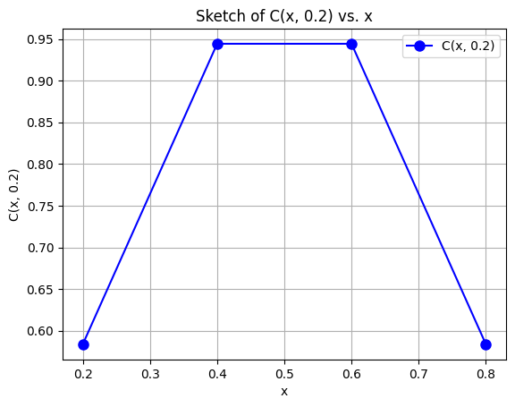 [.45]
[.45]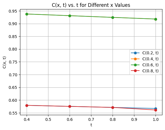
The graph Figure 1(left) illustrates how the value of changes as varies between and . It shows a trend where initially increases from to , remains roughly constant between and , and then decreases back to approximately as increases further.
The graph Figure 1(right) illustrates how the concentration changes over time for different fixed values of x. It shows how the initial concentrations differ and how they evolve as time progresses.
[.45]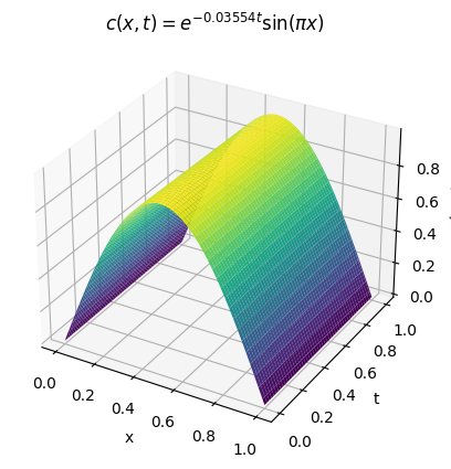 [.45]
[.45]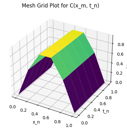
The 3D plot in Figure 2 provides a visual representation of how the function changes with respect to both and . One can observe the combined effect of exponential decay and oscillatory behavior in the resulting surface. From the mesh grid plot, we see that the function is a product of two terms: The first term, , controls the decay as increases. As increases, this term rapidly decreases, indicating that the function becomes smaller as t gets larger. The second term, , introduces oscillations along the -axis. The sine wave causes the surface to rise and fall as varies. As time increases, the oscillations decrease in magnitude, indicating that the function approaches zero for larger values of . This visual representation helps in understanding the behavior of the function in the space.
We developed the code for finite difference method. It generated a mesh grid plot, (Figure 2) to visualize the behavior of the function over a grid defined by spatial dimension with spatial step size and temporal dimension with time step size . The color of the surface plot at each point represents the value of at that specific position and time. Brighter (yellow) colors indicate higher values, while darker (blue) colors indicate lower values.
4 Analysis of concentrations of pollutants through 3D plots
| Pollutants | Diffusivity | Velocity() | |||
|---|---|---|---|---|---|
| Ammonia | |||||
| Carbon monoxide | |||||
| Carbon dioxide | |||||
| Sulphur dioxide |
Analytical
Numerical
[.30]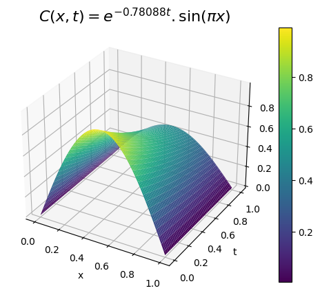 [.30]
[.30]
Analytical
Numerical
[.25]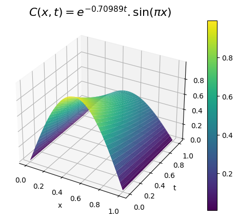 [.25]
[.25]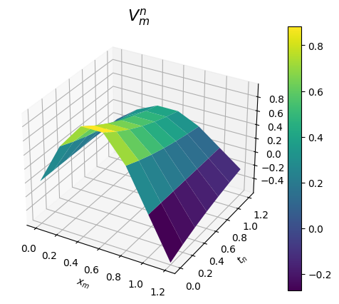
Analytical
Numerical
[.25]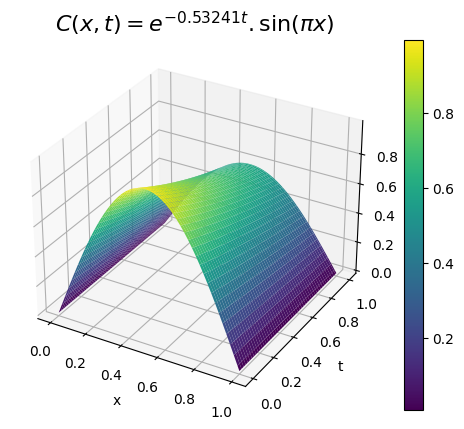 [.25]
[.25]
Analytical
Numerical
[.25]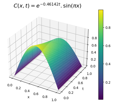 [.25]
[.25]
In this section, we compare the analytical and numerical solution of advection diffusion equation in the case of various pollutants namely Ammonia - , Carbon monoxide - , Carbondioxide - and Sulphur dioxide - [12, 13]. From the above four panels of 3D grapical representations, the concentration of pollutants increases as the diffusivity of the pollutants decreases keeping all other factors influencing concentration like molecular size, pressure, nature of the medium etc. constant.
5 Effect of diffusivity of pollutants
Dividing the spatial interval [0,1] into two equal halves and assuming the pollutants having some diffusivity enters into the region of other pollutants having different diffusivity, keeping the velocity of both the pollutants constant, the one dimensional advection diffusion equation takes the form as follows:
| (34) | |||
where and are the diffusivities of pollutants 1 and 2 respectively. Also let’s consider:
| (35) | |||
First, we consider pollutant 1 be Ammonia and pollutant 2 be Sulphur Dioxide. After that we consider pollutant 1 be Sulphur Dioxide ad pollutant 2 be Ammonia. The diffusivity of Ammonia is and Sulphur Dioxide is . Referring to figure (7), when the pollutant Ammonia having high diffusivity enters into the region of pollutants Sulphur Dioxide having low diffusivity, the concentration of the pollutants increases rapidly. Also the pollutants having low diffusivity, like Sulphur Dioxide enters into the region of the pollutants having high diffusivity like Ammonia, the pollutants flows forward slowly and hence the concentration of the pollutants slowly increase due to high diffusivity of right part of the pollutants.
(a)
(b)
[.45]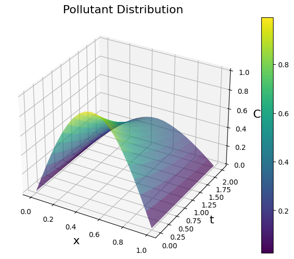 [.45]
[.45]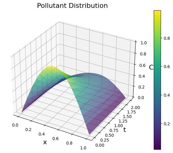
(a)
(b)
[.55]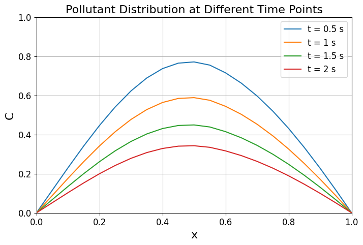 [.55]
[.55]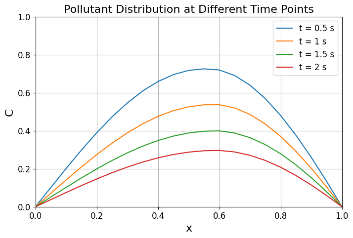
The plot of concentration of pollutants ‘C’ versus ‘x’ at different time levels , and with (a)Ammonia at left and Sulphur Dioxide at right (b) Sulphur Dioxide at left and Ammonia at right. In each time the maximum concentration ‘C’ are around and in figure 8(a) and figure 8(b) respectively.
6 Error Analysis
At and ,
From the table, We have
Error =
At and , From the table , We have
At and ,
From the table , We have
% Error = .
At and , From the table, We have
% Error = .
and so on.
From above calculation, we can observe that the numerical solution by Finite Difference Method for one dimensional advection diffusion equation is very close to its analytical solution and seen to be correct up to four places of decimal. Also, pollutants having higher diffusivity has more error in numerical solution as compared to the analytical solution. Thus, numerical solution is more appropriate in case of pollutants having lower diffusivity. i.e. FTCS scheme gives better approximation for the pollutants having lower diffusivity as compared to the pollutants having higher diffusivity.
7 Conclusion
The study presented a one-dimensional advection-diffusion equation as an illustrative example. Analytical solutions were obtained using the separation of variables method, while a numerical solution was derived through the Forward Time Central Space Scheme (FTCSS). Examining various pollutants (, , and ) with differing diffusivities, it was observed that pollutant concentration increases as diffusivity decreases, assuming constant influencing factors like molecular size, pressure, and medium nature. Treating the atmosphere as a non-homogeneous system, the behavior of pollutants was explored using 2D and 3D plots by equally partitioning high and low diffusivity pollutants in the domain and interchanging them. Notably, when high-diffusivity Ammonia enters the region of low-diffusivity Sulphur Dioxide, pollutant concentration rises rapidly, whereas the entry of low-diffusivity pollutants into high-diffusivity regions results in a gradual increase. Additionally, pollutants with higher diffusivity showed more numerical solution errors compared to analytical solutions, indicating that the FTCS scheme provides a better approximation for pollutants with lower diffusivity.
References
- [1] N. A. Zanudin and Z. M. Isa, “Analytical solutions to advection-diffusion equation with time-fractional caputo-fabrizio derivative.”
- [2] G. Parker, “Encyclopedia of materials: science and technology,” 2001.
- [3] V. Aswin, A. Awasthi, and C. Anu, “A comparative study of numerical schemes for convection-diffusion equation,” Procedia Engineering, vol. 127, pp. 621–627, 2015.
- [4] M. Ahmed, Q. U. A. Zainab, and S. Qamar, “Analysis of one-dimensional advection–diffusion model with variable coefficients describing solute transport in a porous medium,” Transport in Porous Media, vol. 118, pp. 327–344, 2017.
- [5] A. Kumar, D. K. Jaiswal, and N. Kumar, “Analytical solutions of one-dimensional advection-diffusion equation with variable coefficients in a finite domain,” Journal of earth system science, vol. 118, pp. 539–549, 2009.
- [6] J. M. Stockie, “The mathematics of atmospheric dispersion modeling,” Siam Review, vol. 53, no. 2, pp. 349–372, 2011.
- [7] C. Zoppou and J. Knight, “Analytical solutions for advection and advection-diffusion equations with spatially variable coefficients,” Journal of Hydraulic Engineering, vol. 123, no. 2, pp. 144–148, 1997.
- [8] W. A. Strauss, Partial differential equations: An introduction. John Wiley & Sons, 2007.
- [9] S. J. Farlow, Partial differential equations for scientists and engineers. Courier Corporation, 1993.
- [10] B. Grewal and J. Grewal, Numerical Methods in Engineering & Science: With Programs in C, C++ & MATLAB. Khanna, 2014.
- [11] J. Kafle, L. Bagale et al., “Numerical solution of parabolic partial differential equation by using finite difference method,” Journal of Nepal Physical Society, vol. 6, no. 2, pp. 57–65, 2020.
- [12] R. C. Reid, “The properties of gases and liquids thirds edition,” (No Title), pp. 629–665, 1977.
- [13] J. J. McKetta, “Chemical engineers’ handbook (perry, robert h.; chilton, cecil h.; kirkpatrick, sidney d.; ed. s),” 1964.