Prediction De-Correlated Inference

Abstract.

Leveraging machine-learning methods to predict outcomes on some unlabeled datasets and then using these pseudo-outcomes in subsequent statistical inference is common in modern data analysis. Inference in this setting is often called post-prediction inference. We propose a novel, assumption-lean framework for inference under post-prediction setting, called Prediction De-Correlated inference (PDC). Our approach can automatically adapt to any black-box machine-learning model and consistently outperforms supervised methods. The PDC framework also offers easy extensibility for accommodating multiple predictive models. Both numerical results and real-world data analysis support our theoretical results.

1. Introduction

The effectiveness of many modern techniques is heavily reliant on the availability of large amounts of labeled data, which can often be a bottleneck due to the costs associated with data annotation and the scarcity of labeled data in certain domains (Chapelle et al. (2009)). Examples for this situation are ubiquitous, including electronic health records (Cai et al. (2022)), expression quantitative trait loci studies (Michaelson et al. (2009)), public health (Khoury et al. (1999)) among other applications. With the develop of machine learning (ML) and deep learning, predicting the missing outcomes by some ML algorithms, usually black-box models, and using them in subsequent statistical analysis without accounting for the distinction between observed and predicted outcomes is popular in practice. However, this approach heavily relies on the quality of predicted outcomes and can lead to bias in the estimates.

In this article, we study the general semi-supervised M-estimation problem in a post-prediction setting. Suppose we obtain a labeled dataset $\mathcal{D}_{L}:=\{(Y_{i},X_{i}^{T})\in\mathbb{R}\times\mathbb{R}^{p},i=1,\dots,n\}$, each sample is an i.i.d. realization from population $\mathbf{P}_{Y,X}$, and an i.i.d. unlabeled dataset $\mathcal{D}_{U}:=\{X_{i}\in\mathbb{R}^{p},i=n+1,\dots,n+N\}$ from $\mathbf{P}_{X}$ the marginal distribution of $X$. Besides the presence of additional unlabeled data $\mathcal{D}_{U}$, a predictive model $\mu(\cdot)$ independent of $\mathcal{D}_{L}$ and $\mathcal{D}_{U}$ is also available. Wang et al. (2020) also works on this setting. They first use a parametric model to capture the relationship between true labels and predictive model $\mu(\cdot)$, then use this relationship to correct the predictions on the unlabeled data. However, their method requires that the relationship between true labels and $\mu(\cdot)$ can be characterized by a simple parametric model. Recently, Angelopoulos et al. (2023a) propose a general framework called Prediction-Powered Inference (PPI). PPI rectifies the predicted score function and provides valid confidence intervals even using black-box ML models. Besides post-prediction inference, another closely related field is semi-supervised learning. Previous semi-supervised literature mainly focused on special cases of M-estimation problem such as mean estimation (Zhang et al. (2019); Zhang and Bradic (2022)), linear regression (Chakrabortty and Cai (2018); Azriel et al. (2021)), and quantile estimation (Chakrabortty et al. (2022)). More recently, Song et al. (2023) studies the general M-estimation problem and proposes a new estimator via projection technique. The projection basis is polynomial functions of $X$ and the order of polynomial is determined by a $\text{GBIC}_{p}$ procedure (Lv and Liu (2014)). Their method produces asymptotically more efficient estimators for the target parameters than the supervised counterpart. Although the work of Song et al. (2023) is excellent, there are still problems worth solving. If we have extra information about the true model, e.g., a pre-trained model from a different but related large dataset or some suggestions from domain experts, how to use these extra information effectively in a semi-supervised setting is still an open question.

Formally, we aim to perform inference on the parameter $\theta^{*}\in\Theta$, defined as the solution to the estimating equation

(1.1) $$\mathbb{E}\{\mathbf{s}(Y,X,\theta)\}=0,$$

where $\mathbf{s}(Y,X,\theta):\mathbb{R}\times\mathbb{R}^{p}\times\mathbb{R}^{d}\rightarrow\mathbb{R}^{d}$ is a pre-specified score function, the expectation $\mathbb{E}$ is with respect to $\mathbf{P}_{Y,X}$, $\Theta\subset\mathbb{R}^{d}$ and $d$ is some positive integer. Our goal is to propose an estimator that is asymptotically more efficient than the supervised counterpart $\hat{\theta}_{sup}$ which solves the estimating equation $\frac{1}{n}\sum_{i=1}^{n}\mathbf{s}(Y_{i},X_{i},\theta)=0$. It is worth noting that if $\mathbf{s}(Y,X,\theta)=\nabla_{\theta}l(Y,X,\theta)$ for some convex function $l(\cdot,\cdot,\theta)$, then $\theta^{*}$ can also be defined as $\theta^{*}\in\underset{\theta\in\Theta}{\arg\min}\ \mathbb{E}\{l(Y,X,\theta)\}$. However, in this article, we do not assume that this property holds, that is to say, $\mathbf{s}(\cdot,\cdot,\theta)$ may not be written in the form of the gradient of a certain function .

Under some regular conditions, classic statistical theory (Van der Vaart (1998)) implies that the asymptotic covariance of $\hat{\theta}_{sup}$ essentially depends on the properties of the score function at point $\theta^{*}$,

(1.2) $$\sqrt{n}(\hat{\theta}_{sup}-\theta^{*})\overset{p}{\rightarrow}N_{d}(0,[\nabla_{\theta^{T}}\mathbb{E}\{\mathbf{s}(Y,X,\theta^{*})\}]^{-1}{\mathrm{Cov}}(\mathbf{s}(Y,X,\theta^{*}))[\nabla_{\theta}\mathbb{E}\{\mathbf{s}^{T}(Y,X,\theta^{*})\}]^{-1}).$$

Thus, it is reasonable to adjust the empirical score function via $\mathcal{D}_{U}$ and $\mu(\cdot)$. A straightforward approach is to impute the missing labels in $D_{U}$ with $\{\mu(X):X\in\mathcal{D}_{U}\}$ and treat $\mathcal{D}_{L}\cup\{(\mu(X_{i}),X_{i}),i=n+1,\dots,n+N\}$ as the true dataset. Then a supervised approach can be applied to this pseudo dataset to obtain the estimator. The efficiency of this strategy clearly depends on the performance of $\mu(\cdot)$. An inappropriate $\mu(\cdot)$ can result in an estimator that is less efficient than $\hat{\theta}_{sup}$. To solve this problem, Prediction-Powered Inference (PPI)(Angelopoulos et al. (2023a)) uses a debias strategy to rectify the bias caused by the imputed data. They consider the following bias-corrected score function:

$$\hat{S}_{pp}(\theta)=\Big{\{}\underbrace{\frac{1}{n}\sum_{i=1}^{n}\mathbf{s}(Y_{i},X_{i},\theta)-\frac{1}{n}\sum_{i=1}^{n}\mathbf{f}(X_{i},\theta)}_{debiasing\ term}+\frac{1}{N}\sum_{i=n+1}^{n+N}\mathbf{f}(X_{i},\theta)\Big{\}},$$

where $\mathbf{f}(X,\theta)=\mathbf{s}(\mu(X),X,\theta)$ is the predictive score function. $\hat{S}_{pp}(\theta)$ can be seen as $\frac{1}{N}\sum_{i=n+1}^{n+N}\mathbf{f}(X_{i},\theta)$ plus a debiasing term which they called ’rectifier’. This idea has also been studied in semi-supervised literature (Zhang and Bradic (2022); Chakrabortty et al. (2022)) and missing data literature (Robins et al. (1995); Robins and Rotnitzky (1995)). However, it can be verified that, although the estimator $\hat{\theta}_{pp}\in\{\theta:\hat{S}_{pp}(\theta)=0\}$ is asymptotically consistent, it is not always asymptotically efficient than supervised estimator $\hat{\theta}_{sup}$.

1.1. Our Contributions

In this article, we propose a new framework called Prediction De-Correlated inference (PDC) to incorporate the unlabeled data and predictive ML model for M-estimation problem. Our contributions lie in three folds.

• The estimator based on the PDC framework is ’safe’, meaning that even when the black-box ML model makes a poor prediction, the PDC estimator is always asymptotically no worse than its supervised counterpart.

• Our work has unique advantages compared to several existing works. If $\theta^{*}$ is multi-dimensional, one may want to perform inference on $\mathbf{c}^{T}\theta^{*}$ for some vector $\mathbf{c}\in\mathbb{R}^{d}$. Our PDC estimator can provides asymptotically safe estimator for any linear combination of $\theta^{*}$. Existing works (Schmutz et al. (2023); Angelopoulos et al. (2023b); Miao et al. (2023)) are all constrainted to element-wise variance reduction or trace reduction. Our method takes into account the correlation between the components of the estimator, making it a more reliable procedure. For a detailed comparison, see subsection 2.2 and Section 4.

• The proposed PDC framework can be easily extended to accommodate multiple predictive models, see subsection 2.1.

1.2. Organization and Notation

The rest of this article is organized as follows. In Section 2, we describe the proposed Prediction De-Correlated framework. In Section 3, we establish the asymptotic property for the PDC estimator. Numerical studies and a real data analysis are summarized in Section 4. Concluding remarks and discussions for future work are given in Section 5. All technical proofs can be found in Section A.

For any vector $\mathbf{c}$, $\|\mathbf{c}\|$ denotes it’s $L_{2}$ norm. For any matrix $\mathbf{C}$, $\|\mathbf{C}\|$ denotes it’s spectral norm. We add subscript $n$ to $\mathbb{E},\mathrm{Cov}$ to denote the sample version of the population mean and covariance respectively, e.g., $\mathbb{E}_{n}X=\frac{1}{n}\sum_{i=1}^{n}X_{i}$, $\mathrm{Cov}_{n}X=\frac{1}{n}\sum_{i=1}^{n}(X_{i}-\mathbb{E}_{n}X)(X_{i}-\mathbb{E}_{n}X)^{T}$. Similarly, we add subscript $N$ to $\mathbb{E}$ to denote sample version of the population mean based on unlabeled data, e.g. ,$\mathbb{E}_{N}X=\frac{1}{N}\sum_{i=n+1}^{n+N}X_{i}$.

2. Methodology

2.1. Prediction De-Correlated Estimator

Our starting point is to utilize unlabeled data $\mathcal{D}_{U}$ and predictive model $\mu(\cdot)$ to modify the empirical score function, with the aim of reducing (in a matrix sense) the covariance when $\theta=\theta^{*}$. We denote $\mathbf{s}_{1}:=\mathbb{E}_{n}\mathbf{s}(Y,X,\theta),\mathbf{s}_{2}:=\mathbb{E}_{n}\mathbf{f}(X,\theta),\mathbf{s}_{3}:=\mathbb{E}_{N}\mathbf{f}(X,\theta)$. $\mathbf{s}_{1}$ is the empirical score that we use on the supervised inference procedure, which only involves the information from $\mathcal{D}_{L}$. $\mathbf{s}_{2}$ and $\mathbf{s}_{3}$ are the empirical predictive score functions on $\mathcal{D}_{L}$ and $\mathcal{D}_{U}$ respectively, which both utilizes the information from predictive model. Rather than use $\mathbf{s}_{1}$ and $\mathbf{s}_{2}$ to debias $\mathbf{s}_{3}$, we search for a more efficient way to make use of the additional information contained in $\mathcal{D}_{U}$ and $\mu(\cdot)$. We consider solving the following modified estimating equation:

(2.1) $$\mathbf{s}_{1}+\mathbf{A}\mathbf{s}_{2}+\mathbf{B}\mathbf{s}_{3}=\mathbf{0},$$

where $\mathbf{A},\mathbf{B}$ are matrices needed to be specified. Taking the unbiasedness into account, we rewrite it as

$$\mathbf{s}_{1}+\mathbf{T}(\mathbf{s}_{2}-\mathbf{s}_{3})=0,$$

where $\mathbf{T}$ is a matrix needed to be specified. Our goal has shifted to finding the appropriate $\mathbf{T}$ such that the resulting estimator is no worse than the supervised counterpart.

Notice that the nuisance parameter $\mathbf{T}$ is a matrix when $d>1$. It is troublesome to find all the matrices $\mathbf{T}$ such that the resulting estimator is no less efficient than $\hat{\theta}_{sup}$. Now we propose an intuitive choice for $\mathbf{T}$, specifically, $\mathbf{T}=\gamma\widehat{\mathbf{T}}(\theta)$, where

(2.2) $$\widehat{\mathbf{T}}(\theta):=\mathrm{Cov}_{n}(\mathbf{s}_{\theta},\mathbf{f}_{\theta})\{\mathrm{Cov}_{n}(\mathbf{f}_{\theta})\}^{-1}$$

is the sample version of $\mathbf{T}^{*}(\theta):=\mathrm{Cov}(\mathbf{s}_{\theta},\mathbf{f}_{\theta})[\mathrm{Cov}(\mathbf{f}_{\theta})]^{-1}$, $\mathbf{s}_{\theta}:=\mathbf{s}(Y,X,\theta)$, $\mathbf{f}_{\theta}:=\mathbf{f}(X,\theta)$, $\gamma$ is a constant needed to be specified.

The motivation behind this choice of $\mathbf{T}$ is as follows. First, $\mathbf{T}^{*}(\theta^{*})$ is the multivariate least square coefficient matrix, thus $\mathbf{T}^{*}(\theta^{*})\{\mathbf{f}_{\theta^{*}}-\mathbb{E}\mathbf{f}_{\theta^{*}}\}$ is the $L_{2}$ projection of $\mathbf{s}_{\theta^{*}}$ into the linear space spanned by the elements of $\mathbf{f}_{\theta^{*}}-\mathbb{E}\mathbf{f}_{\theta^{*}}$. Hence $S(Y,X,\theta^{*}):=\mathbf{s}_{\theta^{*}}-\mathbf{T}_{\theta^{*}}\{\mathbf{f}_{\theta^{*}}-\mathbb{E}\mathbf{f}_{\theta^{*}}\}$ is the decorrelated score which is orthogonal to $\mathbf{f}_{\theta^{*}}-\mathbb{E}\mathbf{f}_{\theta^{*}}$. The decorrelated score function certainly has a smaller (in a matrix sense) covariance than the original one. The larger the space spanned by $\mathbf{f}_{\theta^{*}}-\mathbb{E}\mathbf{f}_{\theta^{*}}$, the smaller the covariance of the decorrelated score we will obtain. Thus, the dimension of $\mathbf{f}(X,\theta)$ can be different from that of $\mathbf{s}(Y,X,\theta)$. We can augment $\mathbf{f}(X,\theta)$ by another predictive score functions, for example,

$$\mathbf{f}(X,\theta)=(\mathbf{s}^{T}(\mu(X),X,\theta),\mathbf{s}^{T}(\mu_{1}(X),X,\theta))^{T},$$

where $\mu_{1}(\cdot)$ is obtained from another dataset and is different from $\mu(\cdot)$. However, this move needs to be cautious, because we require the covariance matrix of $\mathbf{f}_{\theta^{*}}$ to be invertible.

Since we don’t know $\mathbb{E}\mathbf{f}(X,\theta)$, we need to estimate the centralized $\mathbf{f}(X,\theta)$. Because $\mu(\cdot)$ is independent of $\mathcal{D}_{L}$ and $\mathcal{D}_{U}$, the elements in the set $F(\theta):=\{\mathbf{f}(X_{i},\theta):i=1,\dots,n,\dots,n+N\}$ are exchangeable. Thus, in principle, we can use any subset of $F$ to estimate $\mathbb{E}\mathbf{f}(X,\theta)$, and reserve the rest for projection. In order to increase the correlation between $\mathbf{s}_{1}$ and the projection part, we use the unlabeled data to estimate $\mathbb{E}\mathbf{f}(X,\theta)$. Finally, $\gamma$ is used to adjust for different sample sizes used in $\mathbf{s}_{1}$ and the projection part. Thus, we can estimate $\mathbb{E}S(Y,X,\theta)$ by

(2.3) $$\hat{S}(\theta):=\frac{1}{n}\sum_{i=1}^{n}\Big{[}\{\mathbf{s}(Y_{i},X_{i},\theta)+\gamma\widehat{\mathbf{T}}(\theta)\big{\{}\mathbf{f}(X_{i},\theta)-\frac{1}{N}\sum_{i=n+1}^{n+N}\mathbf{f}(X_{i},\theta)\big{\}}\Big{]}.$$

Solving $\hat{S}(\theta)=0$ directly could result in multiple solutions. So we use an one-step estimator instead. We formalize our one-step Prediction De-Correlated procedure in the following algorithm.

Algorithm 1 Calculate the one-step Prediction De-Correlated estimator $\hat{\theta}_{pdc,1}$

1:Labeled data $\mathcal{D}_{L}$, unlabeled data $\mathcal{D}_{U}$, initial estimator $\hat{\theta}_{0}$, predictive score function $\mathbf{f}(\cdot,\cdot):\mathbb{R}^{p}\times\mathbb{R}^{d}\rightarrow\mathbb{R}^{q}$ for fixed $d,q$.

2:Calculate sample version of the multivariate least square coefficient matrix $\widehat{\mathbf{T}}(\hat{\theta}_{0})$ in (2.2).

3:Calculate the estimated prediction de-correlated score function $\hat{S}(\hat{\theta}_{0})$ in (2.3).

4:Calculate the one-step prediction de-correlated estimator $\hat{\theta}_{pdc}$,

$$\hat{\theta}_{pdc,1}:=\hat{\theta}_{0}-\widehat{\mathbf{H}}^{-1}\hat{S}(\hat{\theta}_{0}).$$

where $\widehat{\mathbf{H}}$ is an estimator of $\mathbf{H}:=\nabla_{\theta^{T}}\mathbb{E}\mathbf{s}(Y,X,\theta^{*})$.

5:One-step Prediction De-Correlated estimator $\hat{\theta}_{pdc,1}$.

The choice of predictive score $\mathbf{f}(X,\theta)$ can be diverse. If the external dataset for training $\mu(\cdot)$ is obtainable, an alternative procedure is to use this dataset to directly estimate the score function when an initial estimator of $\theta^{*}$ is available. Finally, we can use this procedure to update $\hat{\theta}$ iteratively, or just an one-step update.

Example 1 (Mean estimation).

If $s(Y,X,\theta)=Y-\theta$, we are estimating $\mathbb{E}Y$. In this case, $H$ is fixed at 1 therefore we don’t need to estimate it. Choose $\hat{\theta}_{sup}=\mathbb{E}_{n}Y$ as $\hat{\theta}_{0}$, $X$ as $\mathbf{f}(X,\theta)$, then $\hat{S}(\hat{\theta}_{0})=\gamma\mathrm{Cov}_{n}(Y,X)\{\mathrm{Cov}_{n}(X)\}^{-1}(\mathbb{E}_{n}X-\mathbb{E}_{N}X)$. Now $\hat{\theta}_{pdc,1}$ is just the mean estimator proposed by Zhang et al. (2019).

Example 2 (Generalized Linear Models).

In generalized linear models, we have loss function $l(Y,X,\theta)=-YX^{T}\theta+b(X^{T}\theta)$. The corresponding to score function $\mathbf{s}(Y,X,\theta)=-YX+b^{\prime}(X^{T}\theta)X$. We can estimate $\mathbf{H}$ by $\widehat{\mathbf{H}}=\mathbb{E}_{n}\{b^{\prime\prime}(X^{T}\hat{\theta}_{sup})XX^{T}\}$. In linear model, $\mathbf{s}(Y,X,\theta)=(X^{T}\theta-Y)X$, $\widehat{\mathbf{H}}=\mathbb{E}_{n}\{XX^{T}\}$. In logistic model, $s(Y,X,\theta)=-YX+\frac{\exp{X^{T}\theta}}{1+\exp{X^{T}\theta}}X$, $\widehat{\mathbf{H}}=\mathbb{E}_{n}\{\frac{\exp{X^{T}\hat{\theta}_{0}}}{(1+\exp{X^{T}\hat{\theta}_{0}})^{2}}XX^{T}\}$.

2.2. Relationship with Existing literature

Readers may consider applying the above procedure to risk function, that is, minimizing the following modified risk

$$R_{mod}=r_{1}+t(r_{2}-r_{3}),$$

where $r_{1}:=\frac{1}{n}\sum_{i=1}^{n}l(Y_{i},X_{i},\theta)$, $r_{2}:=\frac{1}{n}\sum_{i=1}^{n}l(\mu(X_{i}),X_{i},\theta)$, $r_{3}:=\frac{1}{N}\sum_{i=n+1}^{n+N}l(\mu(X_{i}),X_{i},\theta)$, $t\in\mathbb{R}$ is a scalar determined by the user. This strategy is used in DESSL (Schmutz et al. (2023)) and PPI++ (Angelopoulos et al. (2023b)). Although working on the risk function level is simpler since we only need to find a one-dimensional nuisance $t$, it is a special case of $\mathbf{T}=t\mathbf{I}$ in (2.1). This implies this strategy would loss some generality. On the other hand, both Schmutz et al. (2023) and Angelopoulos et al. (2023b) aim to reduce the trace of the covariance matrix. However, the asymptotic property of the linear combination of the elements of their estimator depends on the specific model and loss function, and it does not guarantee a variance reduction compared with supervised counterpart. The optimal $t$ derived in their paper is

$$t_{opt}=-\eta\frac{\mathrm{Tr}(\mathbf{H}^{-1}(\mathrm{Cov}(\mathbf{s}_{\theta^{*}},\mathbf{f}_{\theta^{*}})+\mathrm{Cov}(\mathbf{f}_{\theta^{*}},\mathbf{s}_{\theta^{*}}))\{\mathbf{H}^{T}\}^{-1})}{2\mathrm{Tr}(\mathbf{H}^{-1}\mathrm{Cov}(\mathbf{f}_{\theta^{*}})\{\mathbf{H}^{T}\}^{-1})},$$

where $\eta$ is the limit of $\frac{N}{n+N}$. By comparing this $t_{opt}$ with $-\eta\mathbf{T}^{*}(\theta^{*})$, we will find that although we need to find a nuisance matrix, our nuisance is easier to calculate.

We notice an independent concurrent work with this article, POst-Prediction Inference (POP-Inf) (Miao et al. (2023)). They also aim to gain efficiency by modifying the score function. But in their setting, datasets $\mathcal{D}_{L}$ and $\mathcal{D}_{U}$ both contain an auxiliary vector $Z$ that is predictive of $Y$, that is $\mathcal{D}_{L}=\{(Y_{i},X_{i},Z_{i}):i=1,\dots,n\}$, $\mathcal{D}_{U}=\{(X_{i},Z_{i}):i=n+1,\dots,n+N\}$, and $\mu(Z)$ produces predictions for $Y$. If $Z\equiv X$, then their settings are the same as ours. In this case, their modified score function is

$$\frac{1}{n}\sum_{i=1}^{n}\mathbf{s}(Y_{i},X_{i},\theta)+\omega\odot\{\frac{1}{n}\sum_{i=1}^{n}\mathbf{f}(X_{i},\theta)-\frac{1}{N}\sum_{i=n+1}^{n+N}\mathbf{f}(X_{i},\theta)\},$$

where $\omega$ is a weighting vector, $\odot$ denotes the element-wise multiplication. This corresponding to $\mathbf{T}=diag(\omega)$ in (2.1). They search for the best $\omega$ by reducing the variance of each element in the estimator successively until the algorithm converges. However, the asymptotic distribution for this estimator (when the iterative times tends to infinity) is unclear. If we assume that the POP-Inf procedure can converge to a consistent estimator of $\theta^{*}$, then intuitively, we can expect it to provide element-wise variance reduction. However, if we need to perform inference on a linear combination of the elements of $\theta$, POP-Inf may no longer provide a guarantee of variance reduction. On the other hand, POP-Inf requires that the dimension of the predictive score function $\mathbf{f}(\cdot,\theta)$ be the same as $\mathbf{s}(\cdot,\cdot,\theta)$, while our PDC procedure can adapt to $\mathbf{f}(\cdot,\theta)$ with any fixed dimension.

3. Theoretical results

In this section, we establish the asymptotic normality for the one-step PDC estimator $\hat{\theta}_{pdc,1}$. We consider two cases where $\mathbf{f}(\cdot,\theta)$ is a deterministic function or a random function, respectively.

3.1. Deterministic predictive model

Before getting down to the business, we need several assumptions.

Assumption 1.

$\theta^{*}$ is an interior point of $\Theta$, where $\Theta$ is a compact subset of $\mathbb{R}^{d}$.

Assumption 2.

$\hat{\theta}_{0}$ is a $\sqrt{n}$-consistent estimator of $\theta^{*}$, that is $\|\hat{\theta}_{0}-\theta^{*}\|=O_{p}(n^{-1/2})$, $\widehat{\mathbf{H}}$ is a consistent estimator of $\mathbf{H}$ such that $\|\widehat{\mathbf{H}}-\mathbf{H}\|=o_{p}(1)$.

Assumption 3.

$\mathbb{E}\{\|\mathbf{s}(Y,X,\theta^{*})\|^{2}\}<\infty$, $\mathbb{E}\{\|\mathbf{f}(X,\theta^{*})\|^{2}\}<\infty$.

Assumption 4.

For every $\theta_{1}$ and $\theta_{2}$ in a neighborhood of $\theta^{*}$, there exists measurable functions $\dot{s}(\cdot,\cdot)$ and $\dot{f}(\cdot)$ with

$$\mathbb{E}\dot{s}^{2}(Y,X)<\infty,\quad\mathbb{E}\dot{f}^{2}(X)<\infty,$$

such that score function $\mathbf{s}(\cdot,\cdot,\theta)$ and predictive score function $\mathbf{f}(\cdot,\theta)$ satisfying the following smoothness condition,

$$\|\mathbf{s}(Y,X,\theta_{1})-\mathbf{s}(Y,X,\theta_{2})\|\leq\dot{s}(Y,X)\|\theta_{1}-\theta_{2}\|,$$

$$\|\mathbf{f}(X,\theta_{1})-\mathbf{f}(X,\theta_{2})\|\leq\dot{f}(X)\|\theta_{1}-\theta_{2}\|.$$

Assumption 5.

$\mathrm{Cov}(\mathbf{f}_{\theta^{*}})$ and $\mathbf{H}$ are nonsingular.

Assumption 1 ensures that $\theta^{*}$ is a reasonable target to estimate. Assumption 2 ensures $\hat{\theta}_{0}$ is a good initial estimator, and can be satisfied by supervised estimator $\hat{\theta}_{sup}$. Assumption 3 enables the use of the central limit theorem. Assumptions 4 -5 are smoothness conditions. Similar assumptions can be found in Van der Vaart (1998). Theorem 1 establishs the asymptotic normality of $\hat{\theta}_{pdc}$.

Theorem 1.

Under Assumptions 1-5, assuming that $\frac{N}{n+N}\rightarrow\eta$ for some constant $\eta\in(0,1]$, then for any fixed $\gamma\in\mathbb{R}$, we have

(3.1) $$\sqrt{n}(\hat{\theta}_{pdc,1}-\theta^{*})\overset{D}{\rightarrow}N_{d}(\mathbf{0},\mathbf{H}^{-1}\bf{\Gamma}(\gamma)\{\mathbf{H}^{T}\}^{-1}),$$

where $\bf{\Gamma}(\gamma)=\mathrm{Cov}\{\mathbf{s}_{\theta^{*}}\}+(\frac{1}{\eta}\gamma^{2}+2\gamma)\mathrm{Cov}(\mathbf{s}_{\theta^{*}},\mathbf{f}_{\theta^{*}})\{\mathrm{Cov}(\mathbf{f}_{\theta^{*}})\}^{-1}\mathrm{Cov}(\mathbf{f}_{\theta^{*}},\mathbf{s}_{\theta^{*}})$.

Remark 1.

By (1.2), we know that $\sqrt{n}(\hat{\theta}_{sup}-\theta^{*})\overset{D}{\rightarrow}N_{d}(0,\mathbf{H}^{-1}\mathrm{Cov}\{\mathbf{s}_{\theta^{*}}\}\{\mathbf{H}^{T}\}^{-1})$. Since

$$\mathrm{Cov}(\mathbf{s}_{\theta^{*}},\mathbf{f}_{\theta^{*}})\{\mathrm{Cov}(\mathbf{f}_{\theta^{*}})\}^{-1}\mathrm{Cov}(\mathbf{f}_{\theta^{*}},\mathbf{s}_{\theta^{*}})$$

is a positive semi-definite matrix, we need $(\frac{1}{\eta}\gamma^{2}+2\gamma)\leq 0$ to obtain an asymptotically more efficient estimator than $\hat{\theta}_{sup}$. Simple mathematical operations gives that:

• When $\gamma\in\{-2\eta,0\}$, $\hat{\theta}_{pdc}$ is asymptotically as efficient as $\hat{\theta}_{sup}$.

• When $\gamma\in(-2\eta,0)$:

  • If $\mathrm{Cov}(\mathbf{s}_{\theta^{*}},\mathbf{f}_{\theta^{*}})\mathrm{Cov}(\mathbf{f}_{\theta^{*}},\mathbf{s}_{\theta^{*}})$ is a positive definite matrix, then $\hat{\theta}_{pdc}$ is asymptotically more efficient than $\hat{\theta}_{sup}$.

  • If $\mathbf{c}^{T}\mathrm{Cov}(\mathbf{s}_{\theta^{*}},\mathbf{f}_{\theta^{*}})\neq\mathbf{0}_{q}$ for a vector $\mathbf{c}\in\mathbb{R}^{d}$, then $\mathbf{c}^{T}\hat{\theta}_{pdc,1}$ is more asymptotically more efficient than $\mathbf{c}^{T}\hat{\theta}_{sup}$. Notice that we have assumed $\eta\neq 0$ in Theorem 1, otherwise we may encounter a case that no PDC estimators are asymptotically more efficient than $\hat{\theta}_{sup}$.

• The optimal $\gamma$ is $\gamma_{opt}=-\eta$, in that case,

  $$\mathbf{\Gamma}(\gamma_{opt})=\mathrm{Cov}\{\mathbf{s}_{\theta^{*}}\}-\eta\cdot\mathrm{Cov}(\mathbf{s}_{\theta^{*}},\mathbf{f}_{\theta^{*}})\{\mathrm{Cov}(\mathbf{f}_{\theta^{*}})\}^{-1}\mathrm{Cov}(\mathbf{f}_{\theta^{*}},\mathbf{s}_{\theta^{*}}).$$

In order to have a more intuitive understanding of Theorem 1, we consider a 1-dimensional case, that is, $d=1$. For $\gamma\in(-2\eta,0)$, we have $\mathbf{\Gamma}(\gamma)-\mathbf{\Gamma}(0)\leq 0$ with equality holds only when $\mathrm{Cov}(\mathbf{s}_{\theta^{*}},\mathbf{f}_{\theta^{*}})=0_{q}$. Since this means the linear space spaned by the elements of $\mathbf{f}_{\theta^{*}}$ is uncorrelated with $\mathbf{s}_{\theta^{*}}$, it is unrealistic to expect gain efficiency via $\mathbf{f}_{\theta^{*}}$. Moreover, in this case, the estimated $\mathbf{T}^{*}(\theta^{*})$, $\hat{\mathbf{T}}(\hat{\theta}_{0})$, should well approach $\mathbf{0}_{1\times q}$ provided that a good initial estimator $\hat{\theta}_{0}$ is used. This data-adaptive weight selection property is the key reason why the PDC estimator is always no worse than the supervised counterpart.

Remark 2.

It is known that when the model is correctly specified in a regression problem, that is, $\mathbb{E}\{\mathbf{s}_{\theta^{*}}|X\}=0$, semi-supervised methods are unable to achieve a smaller asymptotic covariance than $\hat{\theta}_{sup}$ (Kawakita and Kanamori (2013); Song et al. (2023)). The same is true for PDC estimator since in this case $\mathrm{Cov}(\mathbf{s}_{\theta^{*}},\mathbf{f}_{\theta^{*}})=0$ and $\Gamma(\gamma)=\Gamma(0)$. However, it is not true in post-prediction inference. Suppose we have a perfect predictive model. By using this model, we can impute the missing labels, which is equivalent to having labeled samples of size $n+N$. Then, we could get a $\sqrt{n+N}$-consistent estimator of $\theta^{*}$ which is asymptotically superior to $\hat{\theta}_{sup}$. The reason why the PDC estimator does not have this property lies in equation (2.1): we set $\mathbf{A}$ and $\mathbf{B}$ to be equal matrix $\mathbf{T}$ for unbiasedness, while in the perfect prediction case we can set $\mathbf{A}$ and $\mathbf{B}$ to different matrices without breaking the unbiasedness.

Since we know the optimal $\gamma_{opt}$, we need to estimate it in practice. A natural choice is $\gamma_{n}=-\frac{N}{n+N}$. The following corollary provides the asymptotic distribution of $\hat{\theta}_{pdc,1}$ when we set $\gamma$ to $-\frac{N}{n+N}$.

Corollary 1.

Under the conditions of Theorem 1, if we choose $\gamma=-\frac{N}{n+N}$, then

$$\sqrt{n}(\hat{\theta}_{pdc,1}-\theta^{*})\overset{D}{\rightarrow}N_{d}(\mathbf{0},\mathbf{H}^{-1}\boldsymbol{\Gamma}(\gamma_{opt})\{\mathbf{H}^{T}\}^{-1}),$$

3.2. Relationship with Semi-supervised literature

If we choose $\mathbf{f}(X,\theta)$ as some deterministic function $Z(X)$, $\gamma=-\frac{N}{n+N}$, and denote

$$\tilde{Z}(X)\equiv(1,Z(X)^{T})^{T},\mathbf{U}_{n}(\theta)\equiv\mathbb{E}_{n}\{\mathbf{s}(Y,X,\theta)\tilde{Z}(X)^{T}\}\{\mathbb{E}_{n}\tilde{Z}(X)\tilde{Z}(X)^{T}\}^{-1},$$

then

$$\hat{S}(\theta)=\mathbf{U}_{n}(\theta)\frac{1}{n+N}\sum_{i=1}^{n+N}\tilde{Z}(X_{i}).$$

This is equivalent to using the method of Zhang et al. (2019) to estimate each element of $\mathbb{E}\{\mathbf{s}(Y,X,\theta)\}$ based on labeled data $\{(\mathbf{s}(Y_{i},X_{i},\theta),\tilde{Z}(X_{i})),i=1,\dots,n\}$ and unlabeled data $\{\tilde{Z}(X_{i}),i=n+1,\dots,n+N\}$. By the projection property, $\hat{S}(\theta)$ can also be written as

$$\hat{S}(\theta)=\frac{n}{n+N}\sum_{i=1}^{n}\mathbf{s}(Y_{i},X_{i},\theta)+\frac{N}{n+N}\sum_{i=n+1}^{n+N}\mathbf{U}_{n}\tilde{Z}(X_{i}).$$

Searching for the zero point of this $\hat{S}(\theta)$ is equivalent to finding the minimizer of the following modified risk function

$$\hat{R}(\theta)=\frac{n}{n+N}\sum_{i=1}^{n}l(Y_{i},X_{i},\theta)+\frac{N}{n+N}\widehat{\boldsymbol{\beta}}_{l}(\theta)^{T}\tilde{Z}(X_{i}),$$

where $\widehat{\boldsymbol{\beta}}_{l}(\theta)=(\mathbb{E}_{n}\{\tilde{Z}(X)\tilde{Z}(X)^{T}\})^{-1}\mathbb{E}_{n}\{\tilde{Z}(X)l(Y,X,\theta)\}$. This is the weighted loss function in Song et al. (2023) with the optimal weight in their paper. Thus, our PDC procedure can be seen as an extension of the procedure in Song et al. (2023) to accommodate pre-trained ML model. In practice, one can use the semi-supervised estimator obtained by Song et al. (2023) as the initial estimator $\hat{\theta}_{0}$, and then apply the PDC procedure to use the information in $\mathcal{D}_{U}$ more efficiently.

3.3. Confidence Interval

Now we can use $\hat{\theta}_{pdc,1}$ to construct confidence interval for $\mathbf{c}^{T}\theta^{*}$, where $\mathbf{c}$ is any vector from $\mathbb{R}^{d}$.

Corollary 2.

Under the conditions of Theorem 1, the $(1-\alpha)$-level asymptotic confidence interval for $\mathbf{c}^{T}\theta^{*}$ can be written as

$$\Big{[}\mathbf{c}^{T}\hat{\theta}_{pdc,1}-\frac{z_{1-\alpha/2}}{\sqrt{n}}\Big{\{}\mathbf{c}^{T}\widehat{\mathbf{H}}^{-1}\widehat{\mathbf{\Gamma}}(-\frac{N}{n+N})\{\widehat{\mathbf{H}}^{T}\}^{-1}\mathbf{c}\Big{\}}^{1/2},\mathbf{c}^{T}\hat{\theta}_{pdc,1}+\frac{z_{1-\alpha/2}}{\sqrt{n}}\Big{\{}\mathbf{c}^{T}\widehat{\mathbf{H}}^{-1}\widehat{\mathbf{\Gamma}}(-\frac{N}{n+N})\{\widehat{\mathbf{H}}^{T}\}^{-1}\mathbf{c}\Big{\}}^{1/2}\Big{]},$$

where $\widehat{\mathbf{H}}$, $\widehat{\mathbf{\Gamma}}(\gamma)$ are consistent estimators for $\mathbf{H}$, $\mathbf{\Gamma}(\gamma)$ respectively.

For consistent estimators for $\mathbf{H}$ and $\mathbf{\Gamma}(\gamma)$, we can choose

$$\widehat{\mathbf{H}}=\mathbb{E}_{n}\nabla_{\theta^{T}}\mathbf{s}(Y,X,\hat{\theta}),$$

$$\widehat{\mathbf{\Gamma}}(\gamma)=\mathrm{Cov}_{n}\{\mathbf{s}_{\hat{\theta}}\}+(\frac{1}{\eta}\gamma^{2}+2\gamma)\mathrm{Cov}_{n}(\mathbf{s}_{\hat{\theta}},\mathbf{f}_{\hat{\theta}})\{\mathrm{Cov}_{n}(\mathbf{f}_{\hat{\theta}})\}^{-1}\mathrm{Cov}_{n}(\mathbf{f}_{\hat{\theta}},\mathbf{s}_{\hat{\theta}}),$$

where $\hat{\theta}$ is a consistent estimator of $\theta^{*}$. The $\hat{\theta}$ in the above expression can be replaced by any other consistent estimators of $\theta^{*}$, for example, the aforementioned one-step PDC estimator $\hat{\theta}_{pdc,1}$. To fairly compare different estimators, we choose $\hat{\theta}=\hat{\theta}_{sup}$ since it only utilizes the labeled data. Then the $(1-\gamma)$-level asymptotic confidence interval for $\mathbf{c}^{T}\theta^{*}$ constructed by supervised estimator $\hat{\theta}_{sup}$ can be written as

$$\Big{[}\mathbf{c}^{T}\hat{\theta}_{sup}-\frac{z_{1-\alpha/2}}{\sqrt{n}}\Big{\{}\mathbf{c}^{T}\widehat{\mathbf{H}}^{-1}\widehat{\mathbf{\Gamma}}(0)\{\widehat{\mathbf{H}}^{T}\}^{-1}\mathbf{c}\Big{\}}^{1/2},\mathbf{c}^{T}\hat{\theta}_{sup}+\frac{z_{1-\alpha/2}}{\sqrt{n}}\Big{\{}\mathbf{c}^{T}\widehat{\mathbf{H}}^{-1}\widehat{\mathbf{\Gamma}}(0)\{\widehat{\mathbf{H}}^{T}\}^{-1}\mathbf{c}\Big{\}}^{1/2}\Big{]}.$$

3.4. Random predictive model

The predictive score $\mathbf{f}(\cdot,\theta)$ is set to be deterministic function in Theorem 1. However, in practice, black-box ML model could be a random function. We now extend Theorem 1 to accommodate random predictive function. Here, we can rewrite $\mathbf{f}(\cdot,\theta)$ as $\mathbf{f}_{\boldsymbol{\zeta}}(\cdot,\theta)$, where $\boldsymbol{\zeta}$ denote stochastic noise. We need the following assumptions.

Assumption 6.

$\mathbb{E}\{\mathbf{f}_{\boldsymbol{\zeta}}(X,\theta)|X\}=\tilde{\mathbf{f}}(X,\theta)$ for some deterministic function $\tilde{\mathbf{f}}(\cdot,\theta)$, and

$$\mathbf{f}_{\boldsymbol{\zeta}}(X,\theta_{1})-\mathbf{f}_{\boldsymbol{\zeta}}(X,\theta_{2})=\tilde{\mathbf{f}}(X,\theta_{1})-\tilde{\mathbf{f}}(X,\theta_{2})$$

holds almost surely for every $\theta_{1}$ and $\theta_{2}$ in a neighborhood of $\theta^{*}$.

Assumption 6 ensures that the randomness of $\boldsymbol{\zeta}$ does not affect the estimation of $\theta$. In practice, if we choice $\mathbf{f}(X,\theta)$ as $\mathbf{s}(\mu_{\boldsymbol{\zeta}}(X),X,\theta)$ for some random function $\mu_{\boldsymbol{\zeta}}(\cdot)$, then Assumption 6 is satisfied by most common score functions, e.g., the score functions in Example 1, 2.

Assumption 7.

For every $\theta_{1}$ and $\theta_{2}$ in a neighborhood of $\theta^{*}$, there exists measurable functions $\dot{s}(\cdot,\cdot)$ and $\dot{\tilde{f}}(\cdot)$ with

$$\mathbb{E}\dot{s}^{2}(Y,X)<\infty,\quad\mathbb{E}\dot{\tilde{f}}^{2}(X)<\infty,$$

such that score function $\mathbf{s}(\cdot,\cdot,\theta)$ and the conditional expectation of $\mathbf{f}_{\boldsymbol{\zeta}}(X,\theta)$, $\tilde{\mathbf{f}}(X,\theta)$, satisfying the following smoothness condition

$$\|\mathbf{s}(Y,X,\theta_{1})-\mathbf{s}(Y,X,\theta_{2})\|\leq\dot{s}(Y,X)\|\theta_{1}-\theta_{2}\|,$$

$$\|\tilde{\mathbf{f}}(X,\theta_{1})-\tilde{\mathbf{f}}(X,\theta_{2})\|\leq\dot{\tilde{f}}(X)\|\theta_{1}-\theta_{2}\|.$$

Assumption 7 is an adjusted version of Assumption 4 under random predictive model setting.

Theorem 2.

Suppose that Assumptions 1-3, 5, 6-7 hold, and $\frac{N}{n+N}\rightarrow\eta$ for some constant $\eta\in(0,1]$, then for any fixed $\gamma\in\mathbb{R}$, (3.1) still holds.

4. Experiments

4.1. Simulation

In this section, we investigate the numerical performance of PDC estimators in various settings in terms of coverage probability and width of confidence intervals (CI). We compare the performance of PDC estimator to that of three estimators: PPI++ (Because the method DESSL (Schmutz et al. (2023)) and PPI++ (Angelopoulos et al. (2023b)) are almost equivalent in our simulation settings, we only report the results of PPI++.), PPI (Angelopoulos et al. (2023a)), and supervised estimator $\hat{\theta}_{sup}$. Confidence levels are all set to $\alpha=0.1$. Predictive score $\mathbf{f}(X,\theta)$ are all set to $\mathbf{s}(\mu(X),X,\theta)$ for some predictive function $\mu(\cdot)$. All the simulations are repeated for 1000 times.

We analyze the finite sample performance of the aforementioned methods in the following three settings:

1. (Mean estimation) We generate data from model $Y=\beta_{0}+X^{T}\boldsymbol{\beta}+\zeta$, $X\sim N_{2}(0,\mathbf{I}_{2})$, $\zeta\sim N(0,2)$, $(\beta_{0},\boldsymbol{\beta}^{T})$=(2.5, 2.5, -2), labeled data size $n=1000$, unlabeled data size $N=5000$. Predictive model $\mu(X)=(1+\epsilon\cdot\zeta^{\prime})(\beta_{0}+X^{T}\boldsymbol{\beta})$, where $\zeta^{\prime}\sim N(0,1)$, $\epsilon$ are set to different values in $\{0,0.2,0.4,\dots,2\}$ successively.

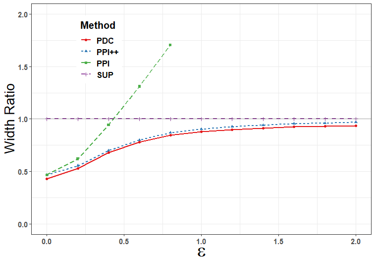
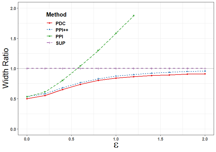
2. (Linear regression) We generate data from model $Y=1+\beta^{T}X-\boldsymbol{\beta}^{T}X^{2}+\boldsymbol{\beta}^{T}X^{3}+\boldsymbol{\beta}^{T}exp(X)+\zeta$, $\zeta\sim N(0,2)$, the elements of $\boldsymbol{\beta}\in\mathbb{R}^{9}$ are generate from $U(2,3)$ or $U(-3,-2)$ except $\beta_{(9)}=0$. $X\sim N_{9}(0,\boldsymbol{\Sigma})$ satisfies $\Sigma_{i,j}=\rho^{|i-j|}$ with $\rho=0$. Predictive model $\mu(X)=(1+\epsilon\cdot\zeta^{\prime})(1+\boldsymbol{\beta}^{T}X-\boldsymbol{\beta}^{T}X^{2}+\boldsymbol{\beta}^{T}X^{3}+\boldsymbol{\beta}^{T}exp(X))$, where $\zeta^{\prime}\sim N(0,1)$, $\epsilon$ are set to different values in $\{0,0.2,0.4,\dots,2\}$ successively.

3. The same setting as setting ii except that $\Sigma_{i,j}=\rho^{|i-j|}$ with $\rho=-0.9$.

For setting i, our goal is to estimate $\theta^{*}=\mathbb{E}Y$. For setting ii and iii, our goal is to estimate $\theta^{*}_{(1)}-\theta^{*}_{(2)}$, where $(\theta^{*}_{(0)},\theta^{*})=\arg\min_{\theta}(Y-(1,X^{T})\theta)^{2}$, a vector with subscript $(i)$ means the $i$-th element of that vector.

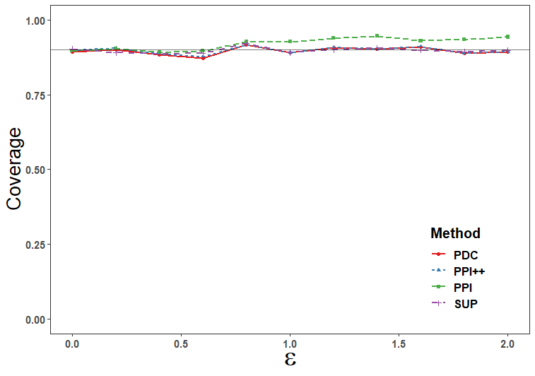
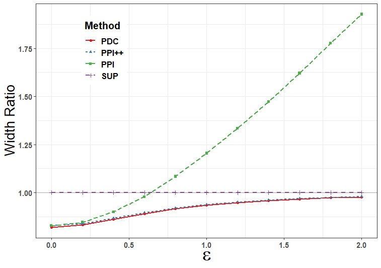
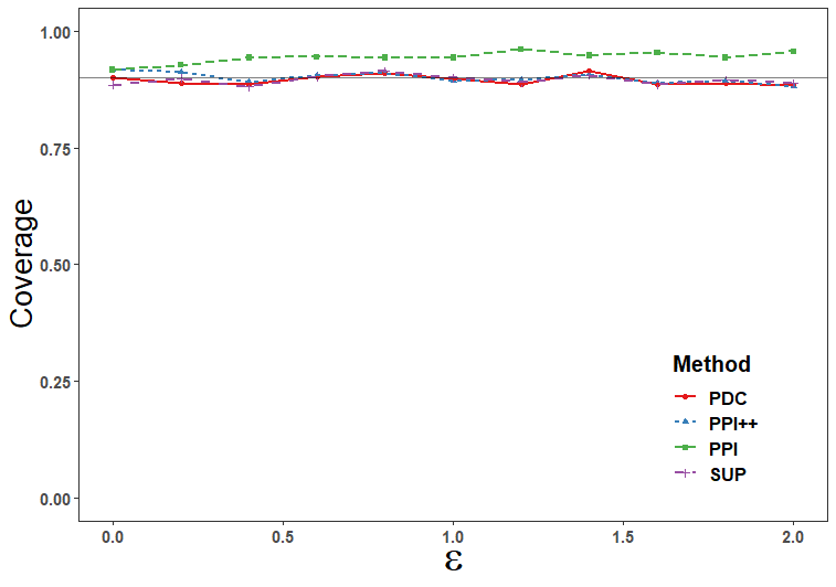
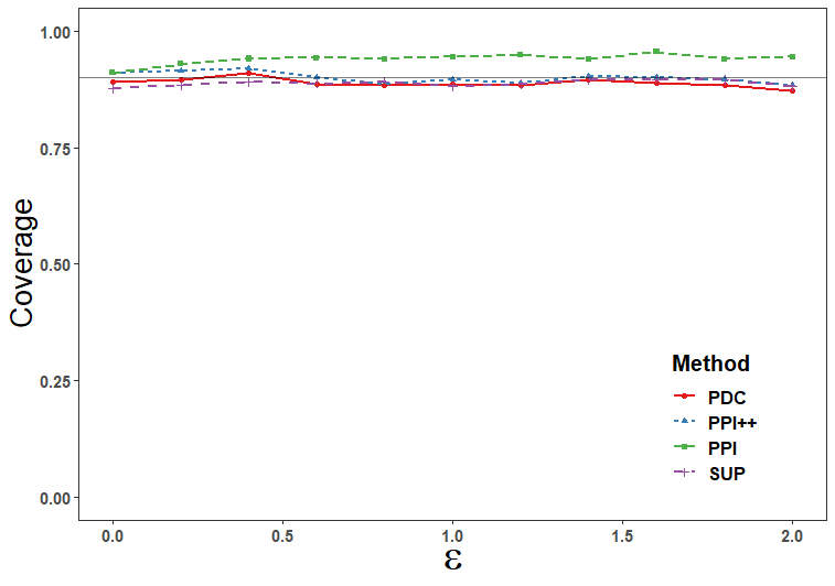
Figure 1 presents the simulation results under setting i. Figure 1(a) shows that all methods guarantee a $(1-\alpha)$-level coverage. However, from figure 1(b), we can see that PPI rapidly deteriorate with the increase of noise level, while PDC and PPI++ always control the standard error (SE). In this case, $\theta^{*}$ is a 1-dimensional target, thus PDC and PPI++ are equivalent. For the results under setting ii and iii, we present the results on coverage in Figure 2 and the the results on width in Figure 3. It is shown in Figure 2 that all methods guarantee the nominal level coverage. On the other hand, Figure 3 shows that PDC estimator is superior to both PPI++ and PPI no matter $\rho=0$ or $\rho=-0.9$. All the experiment results are in agreement with the theoretical analysis in section 3.

(a) Coverage probability for $\mathbb{E}Y$

(b) $\widehat{SE}_{method}/\widehat{SE}_{sup}$

Figure 1. Results under setting i. Figure 1(a) presents the coverage probability of CI constructed by four methods versus noise level $\epsilon$ of predictive model $\mu(\cdot)$. Figure 1(b) presents ratio of the width of different CI to the width of the CI constructed by $\hat{\theta}_{sup}$, versus noise level $\epsilon$.

(a) Coverage for $\theta^{*}_{(1)}-\theta^{*}_{(1)}$ under $\rho=0$.

(b) Coverage for $\theta^{*}_{(1)}-\theta^{*}_{(1)}$ under $\rho=-0.9$

Figure 2. Results on coverage probability under setting ii and iii. Figure 2(a) presents the coverage probability of CI constructed by four methods versus noise level $\epsilon$ of predictive model $\mu(\cdot)$ under setting ii. Figure 2(b) presents the coverage probability under setting iii.

(a) $\widehat{SE}_{method}/\widehat{SE}_{sup}$ under $\rho=0$

(b) $\widehat{SE}_{method}/\widehat{SE}_{sup}$ under $\rho=-0.9$

Figure 3. Results on ratio of the width of different CI to the width of the CI constructed by $\hat{\theta}_{sup}$ under setting ii (Figure 3(a)) and setting iii (Figure 3(b)). The x-axis represents the noise level $\epsilon$ of the predictive function $\mu(\cdot)$.

4.2. Real-world data

We now consider the Los Angeles homeless dataset (Kriegler and Berk (2010)). Our purpose is not to carefully analyze this dataset but rather to demonstrate our new method and to compare it with PPI++, PPI, and the supervised counterpart.

In 2004-2005, the Los Angeles Homeless Services Authority conducted a study of the homeless population. A stratified spatial sampling was used on the 2054 census tracts of Los Angeles County. First, 244 tracts that were believed to have a large amount of homeless were preselected and visited with probability 1. These tracts are known as ”hot tracts.” Next, 265 of the rest non-hot tracts were randomly selected and visited (as $\mathcal{D}_{L}$), leaving 1545 non-hot tracts unvisited (as $\mathcal{D}_{U}$). We include seven predictors recommended by Kriegler and Berk (2010) in our study, Perc.Industrial, Perc.Residential, Perc.Vacant, Perc.Commercial, Perc.OwnerOcc, Perc.Minority, MedianHouseholdIncome. The response variable is Total. Our goal is to estimate the linear regression coefficient on the non-hot tracts.

Although the data from 244 hot tracts are labeled, it is considered to be biased from non-hot tracts. The previous works (Zhang et al. (2019); Azriel et al. (2021); Song et al. (2023)) usually leave out this part of data and only utilize the data from 1810 non-hot tracts. Here we train a random forest (Breiman (2001)) on the data from 244 hot tracts and use this model as predictive function $\mu(\cdot)$. The resulting estimates, as well as the ratio of their $\widehat{SE}$ to $\widehat{SE}_{sup}$ are given in Table 1.

Since the predictive model are training from a different distribution, the performance of PPI is poor, with a much larger standard errors than supervised counterpart, due too the prediction bias. Both PDC and PPI++ produce reasonable estimates. We also notice that the PDC estimator always has a smaller standard error than PPI++ estimator. Another point worth noting is that, in estimation of the coefficient for Perc.Industrial, PPI++ produce an estimator with larger standard error than that of the supervised counterpart. This demonstrates that PPI++ does not guarantee element-wise variance reduction, which is in agreement with our discussions in subsection 2.2.

Table 1. The estimates of coefficients produced by different methods and ratio of their $\widehat{SE}$ to $\widehat{SE}_{sup}$, in the analysis of homeless dataset.

	$\hat{\theta}_{sup}$	$\hat{\theta}_{pdc}$($\widehat{SE}_{pdc}/\widehat{SE}_{sup}$)	$\hat{\theta}_{ppi++}$($\widehat{SE}_{ppi++}/\widehat{SE}_{sup}$)	$\hat{\theta}_{ppi}$($\widehat{SE}_{ppi}/\widehat{SE}_{sup}$)
Intercept	21.964	16.623(0.960)	20.442(0.992)	47.500(2.877)
Perc.Industrial	0.028	-0.014(0.963)	0.031(1.054)	-0.032(3.081)
Perc.Residential	-0.088	-0.109(0.983)	-0.096(0.996)	0.057(3.082)
Perc.Vacant	1.404	1.964(0.826)	1.490(0.940)	-0.040(3.605)
Perc.Commercial	0.339	0.532(0.968)	0.360(0.984)	-0.022(2.140)
Perc.OwnerOcc	-0.233	-0.204(0.937)	-0.209(0.976)	-0.647(2.822)
Perc.Minority	0.059	0.072(0.957)	0.072(0.992)	-0.155(2.510)
MedianInc (in $K)	0.074	0.078(0.844)	0.066(0.898)	0.219(5.040)

5. Discussion

In this article, we propose a novel assumption-lean, model-adaptive approach for post-prediction inference, called Prediction De-Correlated inference. We establish the asymptotic normality of the PDC estimator and compare it with several recent works. The PDC estimator consistently outperforms the competitors and can be extended to accommodate multiple predictive models. Both numerical results and real-world data analysis support our theoretical results.

This article leads to several directions worthy of further investigation. First, the optimal approach to accommodate multiple predictive models is unclear. Second, the PDC procedure can only be applied when the dimension of inference target is fixed, finding a safe alternative under high-dimensional post-prediction settings is valuable.

Appendix A Proofs

We define the empirical notation for any measurable function $g(\cdot)$, $\mathbb{G}_{n}g=\sqrt{n}\{\mathbb{E}_{n}g(Y,X)-\mathbb{E}g(Y,X)\}$, $\mathbb{G}_{N}g=\sqrt{N}\{\mathbb{E}_{N}g(X)-\mathbb{E}g(X)\}$.

Proof of Theorem 1.

First, notice that we can decompose $\hat{\theta}_{pdc,1}$ as follows.

(A.1) $$\begin{split}\sqrt{n}\widehat{\mathbf{H}}(\hat{\theta}_{pdc,1}-\theta^{*})&=\sqrt{n}\widehat{\mathbf{H}}(\hat{\theta}_{0}-\theta^{*})-\sqrt{n}\mathbb{E}_{n}\{\mathbf{s}_{\hat{\theta}_{0}}-\mathbf{s}_{\theta^{*}}\}\\ &\quad-\sqrt{n}\Big{[}\mathbb{E}_{n}\mathbf{s}_{\theta^{*}}+\gamma\mathbf{T}^{*}(\theta^{*})\{\mathbb{E}_{n}\mathbf{f}_{\theta^{*}}-\mathbb{E}_{N}\mathbf{f}_{\theta^{*}}\}\Big{]}\\ &\quad-\sqrt{n}\gamma\mathbf{T}^{*}(\theta^{*})\Big{[}\mathbb{E}_{n}\{\mathbf{f}_{\hat{\theta}_{0}}-\mathbf{f}_{\theta^{*}}\}-\mathbb{E}_{N}\{\mathbf{f}_{\hat{\theta}_{0}}-\mathbf{f}_{\theta^{*}}\}\Big{]}\\ &\quad-\sqrt{n}\gamma(\widehat{\mathbf{T}}(\hat{\theta}_{0})-\mathbf{T}^{*}(\theta^{*}))\Big{[}\mathbb{E}_{n}\mathbf{f}_{\hat{\theta}_{0}}-\mathbb{E}_{N}\mathbf{f}_{\hat{\theta}_{0}}\Big{]}\\ &=I-II-III-IV.\end{split}$$

By Assumption 4 and Example 19.7 in Van der Vaart (1998), we know functions $\{\mathbf{s}(\cdot,\cdot,\theta):\theta\in\Theta\}$ form a $\mathbf{P}_{Y,X}$-Donsker class. Next, Lemma 19.24 of Van der Vaart (1998) implies

(A.2) $$\mathbb{G}_{n}\{\mathbf{s}_{\hat{\theta}_{0}}-\mathbf{s}_{\theta^{*}}\}=o_{p}(1).$$

Hence,

(A.3) $$\mathbb{E}_{n}\{\mathbf{s}_{\hat{\theta}_{0}}-\mathbf{s}_{\theta^{*}}\}=\mathbb{E}\{\mathbf{s}_{\hat{\theta}_{0}}-\mathbf{s}_{\theta^{*}}\}+o_{p}(n^{-1/2}).$$

Thus we can write $I$ as

(A.4) $$\begin{split}I&=\sqrt{n}\widehat{\mathbf{H}}(\hat{\theta}_{0}-\theta^{*})-\sqrt{n}\mathbb{E}\{\mathbf{s}_{\hat{\theta}_{0}}-\mathbf{s}_{\theta^{*}}\}+o_{p}(1)\\ &=\sqrt{n}\widehat{\mathbf{H}}(\hat{\theta}_{0}-\theta^{*})-\sqrt{n}\mathbf{H}(\hat{\theta}_{0}-\theta^{*})+\sqrt{n}o_{p}(\|\hat{\theta}_{0}-\theta^{*}\|)+o_{p}(1)\\ &=o_{p}(1),\end{split}$$

where the second line uses Taylor expansion, the last line follows from Assumption 2.

For $III$, following the same step as deriving (A.2), we have

(A.5) $$\begin{split}\mathbb{E}_{n}\{\mathbf{f}_{\hat{\theta}_{0}}-\mathbf{f}_{\theta^{*}}\}=\mathbb{E}\{\mathbf{f}_{\hat{\theta}_{0}}-\mathbf{f}_{\theta^{*}}\}+n^{-1/2}\mathbb{G}_{n}\{\mathbf{f}_{\hat{\theta}_{0}}-\mathbf{f}_{\theta^{*}}\}=\mathbb{E}\{\mathbf{f}_{\hat{\theta}_{0}}-\mathbf{f}_{\theta^{*}}\}+o_{p}(n^{-1/2}),\\ \mathbb{E}_{N}\{\mathbf{f}_{\hat{\theta}_{0}}-\mathbf{f}_{\theta^{*}}\}=\mathbb{E}\{\mathbf{f}_{\hat{\theta}_{0}}-\mathbf{f}_{\theta^{*}}\}+N^{-1/2}\mathbb{G}_{N}\{\mathbf{f}_{\hat{\theta}_{0}}-\mathbf{f}_{\theta^{*}}\}=\mathbb{E}\{\mathbf{f}_{\hat{\theta}_{0}}-\mathbf{f}_{\theta^{*}}\}+o_{p}(N^{-1/2}).\end{split}$$

Therefore,

(A.6) $$\|III\| \leq\gamma\|\mathbf{T}^{*}(\theta^{*})\|\Big{\|}\mathbb{G}_{n}\{\mathbf{f}_{\hat{\theta}_{0}}-\mathbf{f}_{\theta^{*}}\}-\sqrt{\frac{n}{N}}\mathbb{G}_{N}\{\mathbf{f}_{\hat{\theta}_{0}}-\mathbf{f}_{\theta^{*}}\}\Big{\|}=o_{p}(1).$$

For $IV$, we decompose $\|IV\|$ as two terms,

(A.7) $$\|IV\|\leq\sqrt{n}\gamma\|\widehat{\mathbf{T}}(\hat{\theta}_{0})-\mathbf{T}^{*}(\theta^{*})\|\Big{\|}\mathbb{E}_{n}\{f_{\hat{\theta}_{0}}-f_{\theta^{*}}\}-\mathbb{E}_{N}\{f_{\hat{\theta}_{0}}-f_{\theta^{*}}\}\Big{\|}$$

$$\quad+\sqrt{n}\gamma\|\widehat{\mathbf{T}}(\hat{\theta}_{0})-\mathbf{T}^{*}(\theta^{*})\|\Big{\|}\mathbb{E}_{n}f_{\theta^{*}}-\mathbb{E}_{N}f_{\theta^{*}}\Big{\|}.$$

We consider $\|\widehat{\mathbf{T}}(\hat{\theta}_{0})-\mathbf{T}^{*}(\theta^{*})\|$ first. We have

(A.8) $$\|\widehat{\mathbf{T}}(\hat{\theta}_{0})-\mathbf{T}^{*}(\theta^{*})\|\leq\|\widehat{\mathbf{T}}(\hat{\theta}_{0})-\hat{\mathbf{T}}(\theta^{*})\|+\|\widehat{\mathbf{T}}(\theta^{*})-\mathbf{T}^{*}(\theta^{*})\|.$$

Since $d$ is fixed, the law of large numbers implies the second part on the right-hand side is a small term, that is

(A.9) $$\|\widehat{\mathbf{T}}(\theta^{*})-\mathbf{T}^{*}(\theta^{*})\|=o_{p}(1).$$

For the first part,

$$\|\widehat{\mathbf{T}}(\hat{\theta}_{0})-\widehat{\mathbf{T}}(\theta^{*})\| \leq\|\mathrm{Cov}_{n}(\mathbf{s}_{\hat{\theta}_{0}},\mathbf{f}_{\hat{\theta}_{0}})[\{\mathrm{Cov}_{n}(\mathbf{f}_{\hat{\theta}_{0}})\}^{-1}-\{\mathrm{Cov}_{n}(\mathbf{f}_{\theta^{*}})\}^{-1}]\|$$

(A.10) $$\quad+\|[\mathrm{Cov}_{n}(\mathbf{s}_{\hat{\theta}_{0}},\mathbf{f}_{\hat{\theta}_{0}})-\mathrm{Cov}_{n}(\mathbf{s}_{\theta^{*}},\mathbf{f}_{\theta^{*}})]\{\mathrm{Cov}_{n}(\mathbf{f}_{\theta^{*}})\}^{-1}\|.$$

Observe that

$$\mathrm{Cov}_{n}(\mathbf{s}_{\hat{\theta}_{0}},\mathbf{f}_{\hat{\theta}_{0}})-\mathrm{Cov}_{n}(\mathbf{s}_{\theta^{*}},\mathbf{f}_{\theta^{*}}) =\mathbb{E}_{n}\{\mathbf{s}_{\hat{\theta}_{0}}\mathbf{f}_{\hat{\theta}_{0}}^{T}\}-\mathbb{E}_{n}\{\mathbf{s}_{\theta^{*}}\mathbf{f}_{\theta^{*}}^{T}\}$$

$$\quad-[\{\mathbb{E}_{n}\mathbf{s}_{\hat{\theta}_{0}}\}\{\mathbb{E}_{n}\mathbf{f}_{\hat{\theta}_{0}}\}^{T}-\{\mathbb{E}_{n}\mathbf{s}_{\theta^{*}}\}\{\mathbb{E}_{n}\mathbf{f}_{\theta^{*}}\}^{T}]$$

$$:=\mathbf{C}_{1}-\mathbf{C}_{2},$$

For $\mathbf{C}_{1}$, we decompose it as

$$\mathbf{C}_{1} =\mathbb{E}_{n}[\{\mathbf{s}_{\hat{\theta}_{0}}-\mathbf{s}_{\theta^{*}}\}\mathbf{f}_{\theta^{*}}^{T}]+\mathbb{E}_{n}[\{\mathbf{s}_{\hat{\theta}_{0}}-\mathbf{s}_{\theta^{*}}\}\{\mathbf{f}_{\hat{\theta}_{0}}-\mathbf{f}_{\theta^{*}}\}^{T}]+\mathbb{E}_{n}[\mathbf{s}_{\theta^{*}}\{\mathbf{f}_{\hat{\theta}_{0}}-\mathbf{f}_{\theta^{*}}\}^{T}]$$

(A.11) $$:=\mathbf{C}_{11}+\mathbf{C}_{12}+\mathbf{C}_{13}.$$

By Assumption 3-4, we have

(A.12) $$\|\mathbf{C}_{11}\|\leq\mathbb{E}_{n}[\|\mathbf{s}_{\hat{\theta}_{0}}-\mathbf{s}_{\theta^{*}}\|\cdot\|\mathbf{f}_{\theta^{*}}\|]\leq\|\hat{\theta}_{0}-\theta^{*}\|\mathbb{E}_{n}\{\dot{s}\cdot\|\mathbf{f}_{\theta^{*}}\|\}=O_{p}(n^{-1/2}),$$

(A.13) $$\|\mathbf{C}_{13}\|\leq\mathbb{E}_{n}[\|\mathbf{f}_{\hat{\theta}_{0}}-\mathbf{f}_{\theta^{*}}\|\cdot\|\mathbf{s}_{\theta^{*}}\|]\leq\|\hat{\theta}_{0}-\theta^{*}\|\mathbb{E}_{n}\{\dot{f}\cdot\|\mathbf{s}_{\theta^{*}}\|\}=O_{p}(n^{-1/2}),$$

(A.14) $$\|\mathbf{C}_{12}|\leq\mathbb{E}_{n}\|\mathbf{s}_{\hat{\theta}_{0}}-\mathbf{s}_{\theta^{*}}\|\|\mathbf{f}_{\hat{\theta}_{0}}-\mathbf{f}_{\theta^{*}}\|\leq\mathbb{E}_{n}\{\dot{s}\cdot\dot{f}\}\|\hat{\theta}_{0}-\theta^{*}\|^{2}=O_{p}(n^{-1}).$$

On the other hand, (A.3) and (A.5) together imply that

(A.15) $$\mathbf{C}_{2}=\{\mathbb{E}_{n}\mathbf{s}_{\theta^{*}}+o_{p}(1)\}\{\mathbb{E}\mathbf{f}_{\theta^{*}}+o_{p}(1)\}^{T}-\{\mathbb{E}_{n}\mathbf{s}_{\theta^{*}}\}\{\mathbb{E}_{n}\mathbf{f}_{\theta^{*}}\}^{T}=o_{p}(1).$$

Combing (A)-(A.15) yields

(A.16) $$\mathrm{Cov}_{n}(\mathbf{s}_{\hat{\theta}_{0}},\mathbf{f}_{\hat{\theta}_{0}})-\mathrm{Cov}_{n}(\mathbf{s}_{\theta^{*}},\mathbf{f}_{\theta^{*}})=o_{p}(1).$$

Since $d$ is fixed, by law of large numbers we have $\mathrm{Cov}_{n}(\mathbf{s}_{\theta^{*}},\mathbf{f}_{\theta^{*}})\overset{p}{\rightarrow}\mathrm{Cov}(\mathbf{s}_{\theta^{*}},\mathbf{f}_{\theta^{*}})$. This, combined with (A.16) implies that

(A.17) $$\mathrm{Cov}_{n}(\mathbf{s}_{\hat{\theta}_{0}},\mathbf{f}_{\hat{\theta}_{0}})=O_{p}(1).$$

Following the same procedure, we can prove

(A.18) $$\begin{split}\mathrm{Cov}_{n}(\mathbf{f}_{\theta^{*}})=\mathrm{Cov}(\mathbf{f}_{\theta^{*}})+o_{p}(1),\\ \mathrm{Cov}_{n}(\mathbf{f}_{\hat{\theta}_{0}})=\mathrm{Cov}(\mathbf{f}_{\theta^{*}})+o_{p}(1).\end{split}$$

Since the elements of the matrix inverse are continuous functions of the original matrix elements, (A.18) imply that

(A.19) $$\{\mathrm{Cov}_{n}(\mathbf{f}_{\hat{\theta}_{0}})\}^{-1}-\{\mathrm{Cov}_{n}(\mathbf{f}_{\theta^{*}})\}^{-1}=o_{p}(1),\quad\{\mathrm{Cov}_{n}(\mathbf{f}_{\theta^{*}})\}^{-1}=\{\mathrm{Cov}(\mathbf{f}_{\theta^{*}})\}^{-1}+o_{p}(1).$$

Hence, (A), (A.16),(A.17),(A.19) together imply that

(A.20) $$\|\widehat{\mathbf{T}}(\hat{\theta}_{0})-\hat{\mathbf{T}}(\theta^{*})\|=o_{p}(1).$$

Combing (A.8), (A.20), (A.9), we have shown that

(A.21) $$\|\widehat{\mathbf{T}}(\hat{\theta}_{0})-\mathbf{T}^{*}(\theta^{*})\|=o_{p}(1).$$

For the rest term in the decomposition of $\|IV\|$, by multivariate central limit theorem,

$$\sqrt{n}\|\mathbb{E}_{n}\mathbf{f}_{\theta^{*}}-\mathbb{E}_{N}\mathbf{f}_{\theta^{*}}\|=O_{p}(1).$$

This, combined with (A.7), (A.21), (A.5), imply that

(A.22) $$\|IV\|=o_{p}(1).$$

Since $\mathcal{D}_{L}$ are independent of $\mathcal{D}_{U}$, by multivariate central limit theorem,

(A.23) $$II\overset{D}{\rightarrow}N_{d}(\mathbf{0},\mathbf{\Gamma}(\gamma)).$$

Combing (A.1), (A.4), (A.6), (A.22), (A.23), we have shown that

$$\sqrt{n}\widehat{\mathbf{H}}(\hat{\theta}_{m}-\theta^{*})\overset{D}{\rightarrow}N_{d}(\mathbf{0},\boldsymbol{\Gamma}(\gamma)).$$

Finally, by Slutsky’s theorem and Assumption 2, we have completed the proof. ∎

Proof of Theorem 2.

Similar to equation (A.1), we decompose $\sqrt{n}\widehat{\mathbf{H}}(\hat{\theta}_{pdc,1}-\theta^{*})$ as

$$\sqrt{n}\widehat{\mathbf{H}}(\hat{\theta}_{pdc,1}-\theta^{*}) =I-II$$

$$\quad-\sqrt{n}\gamma\mathbf{T}^{*}(\theta^{*})\Big{[}\mathbb{E}_{n}\{\tilde{\mathbf{f}}_{\hat{\theta}_{0}}-\tilde{\mathbf{f}}_{\theta^{*}}\}-\mathbb{E}_{N}\{\tilde{\mathbf{f}}_{\hat{\theta}_{0}}-\tilde{\mathbf{f}}_{\theta^{*}}\}\Big{]}$$

$$\quad-\sqrt{n}\gamma(\widehat{\mathbf{T}}(\hat{\theta}_{0})-\mathbf{T}^{*}(\theta^{*}))\Big{[}\mathbb{E}_{n}\tilde{\mathbf{f}}_{\hat{\theta}_{0}}-\mathbb{E}_{N}\tilde{\mathbf{f}}_{\hat{\theta}_{0}}\Big{]}:=I-II-\tilde{III}-\tilde{IV}.$$

By Assumption 6, the proof follows the same procedure as that of Theorem 1. ∎

Proof of Corollary 1.

We denote the one-step PDC estimator when $\gamma=\gamma_{n}$ as $\hat{\theta}_{pdc,1}(\gamma_{n})$. We can still use the decomposition in equation (A.1). We brief denote the decomposition as $\sqrt{n}\hat{\mathbf{H}}(\hat{\theta}_{pdc,1}(\gamma_{n})-\theta^{*})=I-II_{n}-III_{n}-IV_{n}$. $I$ is same as the one in fixed $\gamma$ case. Since $\gamma_{n}$ is bounded, we still have $III_{n}=o_{p}(1)$ and $IV_{n}=o_{p}(1)$. For $II_{n}$, we have

$$II_{n}-II=(\gamma_{n}-\gamma_{opt})\sqrt{n}\mathbf{T}^{*}(\theta^{*})\{\mathbb{E}_{n}\mathbf{f}_{\theta^{*}}-\mathbb{E}_{N}\mathbf{f}_{\theta^{*}}\}=(\gamma_{n}-\gamma_{opt})O_{p}(1)=o_{p}(1).$$

Thus we have completed the proof. ∎

References

• Angelopoulos et al. (2023a) Angelopoulos, A. N., Bates, S., Fannjiang, C., Jordan, M. I., and Zrnic, T. (2023a), “Prediction-powered inference,” Science, 382, 669–674.
• Angelopoulos et al. (2023b) Angelopoulos, A. N., Duchi, J. C., and Zrnic, T. (2023b), “PPI++: Efficient Prediction-Powered Inference,” arXiv preprint arXiv:2311.01453.
• Azriel et al. (2021) Azriel, D., Brown, L. D., Sklar, M., Berk, R., Buja, A., and Zhao, L. (2021), “Semi-supervised linear regression,” Journal of the American Statistical Association, 1–14.
• Breiman (2001) Breiman, L. (2001), “Random forests,” Machine Learning, 45, 5–32.
• Cai et al. (2022) Cai, T., Li, M., and Liu, M. (2022), “Semi-supervised Triply Robust Inductive Transfer Learning,” arXiv preprint arXiv:2209.04977.
• Chakrabortty and Cai (2018) Chakrabortty, A. and Cai, T. (2018), “Efficient and adaptive linear regression in semi-supervised settings,” The Annals of Statistics, 46, 1541 – 1572.
• Chakrabortty et al. (2022) Chakrabortty, A., Dai, G., and Carroll, R. J. (2022), “Semi-Supervised Quantile Estimation: Robust and Efficient Inference in High Dimensional Settings,” arXiv preprint arXiv:2201.10208.
• Chapelle et al. (2009) Chapelle, O., Schölkopf, B., and Zien, A. (2009), Semi-supervised Learning, MIT Press.
• Kawakita and Kanamori (2013) Kawakita, M. and Kanamori, T. (2013), “Semi-supervised learning with density-ratio estimation,” Machine Learning, 91, 189–209.
• Khoury et al. (1999) Khoury, S., Massad, D., and Fardous, T. (1999), “Mortality and causes of death in Jordan 1995-96: assessment by verbal autopsy.” Bulletin of the World Health Organization, 77, 641.
• Kriegler and Berk (2010) Kriegler, B. and Berk, R. (2010), “Small area estimation of the homeless in Los Angeles: An application of cost-sensitive stochastic gradient boosting,” The Annals of Applied Statistics, 4, 1234–1255.
• Lv and Liu (2014) Lv, J. and Liu, J. S. (2014), “Model selection principles in misspecified models,” Journal of the Royal Statistical Society Series B: Statistical Methodology, 76, 141–167.
• Miao et al. (2023) Miao, J., Miao, X., Wu, Y., Zhao, J., and Lu, Q. (2023), “Assumption-lean and Data-adaptive Post-Prediction Inference,” arXiv preprint arXiv:2311.14220.
• Michaelson et al. (2009) Michaelson, J. J., Loguercio, S., and Beyer, A. (2009), “Detection and interpretation of expression quantitative trait loci (eQTL),” Methods, 48, 265–276.
• Robins and Rotnitzky (1995) Robins, J. M. and Rotnitzky, A. (1995), “Semiparametric efficiency in multivariate regression models with missing data,” Journal of the American Statistical Association, 90, 122–129.
• Robins et al. (1995) Robins, J. M., Rotnitzky, A., and Zhao, L. P. (1995), “Analysis of semiparametric regression models for repeated outcomes in the presence of missing data,” Journal of the American Statistical Association, 90, 106–121.
• Schmutz et al. (2023) Schmutz, H., Humbert, O., and Mattei, P.-A. (2023), “Don’t fear the unlabelled: safe semi-supervised learning via debiasing,” in The Eleventh International Conference on Learning Representations.
• Song et al. (2023) Song, S., Lin, Y., and Zhou, Y. (2023), “A General M-estimation Theory in Semi-Supervised Framework,” Journal of the American Statistical Association, 1–11.
• Van der Vaart (1998) Van der Vaart, A. W. (1998), Asymptotic Statistics, Cambridge Series in Statistical and Probabilistic Mathematics, Cambridge University Press.
• Wang et al. (2020) Wang, S., McCormick, T. H., and Leek, J. T. (2020), “Methods for correcting inference based on outcomes predicted by machine learning,” Proceedings of the National Academy of Sciences, 117, 30266–30275.
• Zhang et al. (2019) Zhang, A., Brown, L. D., and Cai, T. T. (2019), “Semi-supervised inference: General theory and estimation of means,” The Annals of Statistics, 47, 2538 – 2566.
• Zhang and Bradic (2022) Zhang, Y. and Bradic, J. (2022), “High-dimensional semi-supervised learning: in search of optimal inference of the mean,” Biometrika, 109, 387–403.