$\Gamma$-Convergence for plane to wrinkles transition problem

Abstract

We consider a variational problem modeling transition between flat and wrinkled region in a thin elastic sheet, and identify the $\Gamma$-limit as the sheet thickness goes to $0$, thus extending the previous work of the first author [Bella, ARMA 2015]. The limiting problem is scalar and convex, but constrained and posed for measures. For the $\Gamma-\liminf$ inequality we first pass to quadratic variables so that the constraint becomes linear, and then obtain the lower bound using Reshetnyak’s theorem. The construction of the recovery sequence for the $\Gamma-\limsup$ inequality relies on mollification of quadratic variables, and careful choice of multiple construction parameters. Eventually for the limiting problem we show existence of a minimizer and equipartition of the energy for each frequency.

1 Introduction

This paper is about fine analysis of minimizers of a nonconvex variational problem which describes wrinkling of thin elastic sheets.

Motivated by some physical experiments with thin elastic sheets [22, 23, 24], the first author, in his PhD thesis [8] (see also [5]), considered a specific variational problem describing deformations of a thin elastic sheet $\Omega_{h}\subset\mathbb{R}^{3}$ of thickness $h$ and cross section of annular shape. The elastic energy, corresponding to a deformation $v\colon\Omega_{h}\to\mathbb{R}^{3}$, consists of a membrane term, measuring stretching and compression of the sheet, and of a bending term, which penalizes curvature. As a proxy for the energy one can think of

$$E_{h}(v)=\int_{\Omega_{h}}\mathrm{dist}^{2}(\nabla v,{\mathrm{SO}}(3))\,{\rm d}x+h^{2}\int_{\Omega_{h}}|\nabla^{2}v|^{2}\,{\rm d}x.$$ (1.1)

The membrane part is non-convex, possibly giving rise to oscillations. In contrast, the latter bending part is convex and of higher-order, thus regularizing the problem. Since the bending resistance is related to the sheet thickness $h$, the magnitude of this contribution asymptotically vanishes in the limit $h\searrow 0$.

The physics approach to tackle these problems consists of a specific choice of an ansatz (guess) for the form (shape) of a minimizer. In other words, one restricts the analysis to a class of competitors having specific characteristics, and look for a minimizer of the energy within that class. On the other hand, the rigorous analytical approach does not make any assumptions on the form of a minimizer, i.e., the energy is minimized over all possible deformations. The problem in (1.1) being non-convex, hence possibly possessing many (local) minimizers or critical points, the first step is to understand the minimal value of the energy, with possibly learning some clues by which deformations is this minimal value, at least approximately, achieved.

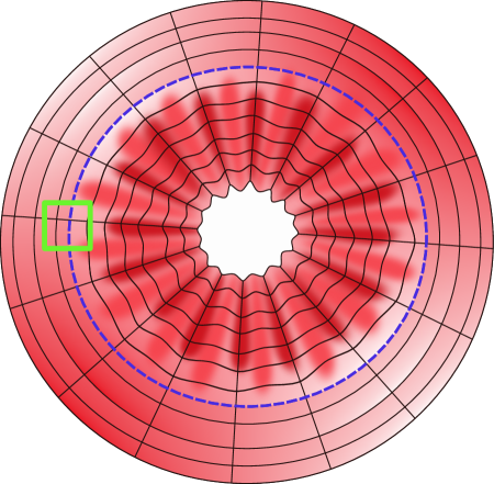
Figure 1: Elastic annular membrane stretched in the radial direction. The blue dotted curve represents the free boundary that separates the outer stretched region from the inner wrinkled one.

Hence, we first try to identify the minimal value of the energy. Precisely, in the present situation, the goal is to understand its dependence on the (small) sheets thickness $h$. It turns out that the minimal value $\min_{v}E_{h}(v)$ consists of a leading zeroth-order term $\mathcal{E}_{0}$ (coming from the stretching of the sheet) plus a linear correction in $h$, which corresponds to the cost of wrinkling of the sheet [8, 5]. More precisely, there exist two constants $0<C_{0}<C_{1}<\infty$ such that for any thickness $0<h<1$ there holds

$$\mathcal{E}_{0}+C_{0}h\leq\min_{v}E_{h}(v)\leq\mathcal{E}_{0}+C_{1}h.$$ (1.2)

The wrinkling serves as a mechanism to relieve compressive stresses, which are caused by specific geometrical effects. An alternative to wrinkling would be simply compression, which contributes to the membrane part at the order $O(1)$. Hence, in the case of small thickness (present situation) compression is much less energetically favorable ($O(1)$ vs $O(h^{2})$), and thus not expected.

The identified linear scaling law (1.2) in $h$ for the minimal value of the energy raised a lot of discussion among the physics community, having improved their ansatz-based prediction by a factor of $\log h$ (i.e. $h$ in [5] vs $h{(|\log h|+1)}$ in [22]). It turns out that this discrepancy is related to a suboptimal choice of the ansatz close to the interface between the wrinkled and the flat region. Moreover, the upper bound in (1.2) is achieved through a complex construction involving branching effects, a pattern which was not observed experimentally.

To shed light on this discrepancy, the first author considered a variational problem modelling the transition region [9] with the aim of better understanding the behavior of the minimizer in that region. Working at the level of the energy, this means to consider the quantity $\frac{\min_{u}E_{h}(u)-\mathcal{E}_{0}}{h}$, which not only is bounded away from $0$ and $\infty$ (see (1.2)), but as $h\searrow 0$ it actually converges to some value $\sigma$ (as proven in [9]). Even though the value $\sigma$ is characterized as a limit of minima of simpler scalar and convex variational problems, it does not provide any information on the form of sequence of minimizers.

In that respect, the goal of this paper is to overcome this shortcoming by showing $\Gamma$-convergence of the functionals $\frac{E_{h}-\mathcal{E}_{0}}{h}$ as $h\searrow 0$. As usual, a consequence of $\Gamma$-convergence is convergence of minimizers $u_{h}$ of $E_{h}$ to a minimizer of the limiting problem, hence providing information on $u_{h}$, at least for $0<h\ll 1$. Denoting by $\mathcal{F}_{\infty}$ the $\Gamma$-limit functional (see (2.9) below), it turns out that as expected from [9], $\mathcal{F}_{\infty}$ is scalar and convex, thus possibly much easier to analyze than the original $E_{h}$. Nevertheless, the study of minimizers of $\mathcal{F}_{\infty}$ is still far from trivial and we postpone it to a future work – except for some preliminary results collected in Section 6.

There are many areas of material science, most of them falling within a class of energy-driven pattern formation [29], where the idea to study energy scaling laws for variational problems turned out to be very fruitful. The common features of these problems is the presence of a nonconvex term in the energy, which is regularized by a higher-order term with a small prefactor. This small parameter (for now denoted $\varepsilon$) has different meanings: thickness in the case of elastic films, inverse Ginzburg-Landau parameter in the theory of superconductors, strength of the interfacial energy for models of shape-memory alloys or micromagnetics, to name just few. As $\varepsilon\searrow 0$, the oscillations caused by the nonconvexity are less penalized, giving the energy more freedom to form patterns/microstructure.

The first paper in this direction, in the context of shape memory alloys, is a seminal work of Kohn and Müller [28], where they studied a toy problem to model the interface in the austenite-martensite phase transformation. They showed that the energy minimum scales like $\epsilon^{2/3}$, which was in contrast with the scaling $\varepsilon^{1/2}$, widely accepted in the physics community. More precisely, the physics arguments were based on an ansatz of “one-dimensional” structure of minimizers, whereas Kohn and Müller used a branching construction to achieve lower energy. While they did not show the form of minimizers, they provided localized (in one direction) estimates on the energy distribution for the minimizer – thus providing hints on scales used for branching. Subsequently, Conti [20] used an intricate upper bound construction to show localized energy bounds (in both directions), which in particular implies asymptotical self-similarity of the minimizer close to the interface. The analysis of the toy model was later generalized in several directions, for example analysis based on energy scalings laws for the cubic-to-tetragonal phase transformation - e.g. rigidity of the microstructure [17, 18] or study of the energy barrier for the nucleation in the bulk [27] and at the boundary [3]. In that respect it is worth to also mention recent works of Rüland and Tribuzio [44, 43], where a novel use of Fourier Analysis allows to obtain sharp lower bounds on the energy on a more advanced model.

The work of Kohn and Müller initiated many developments in other areas of material science to study pattern formation driven by the energy minization, for example in micromagnetics [37, 16, 41], island growth on epitaxially strained films [4], diblock copolymers [19], optimal design [33, 32], or superconductors [46]. Picking one of them as an example, the Ginzburg-Landau model describes behavior of superconductors in different regimes of the applied magnetics field. While for extreme values of the magnetic field (very small or very large) there is only one (normal or superconducting) phase, for intermediate values of the field the mixed states consisting of many vortices are observed. There the leading order energy characterizes the number of vortices, and the next order in the energy describes interaction between them (see [46] for a survey, [42] for analysis in three spatial dimensions, and [39] for a similar work in the context of $2d$ Coulomb gases).

The models for wrinkling of thin elastic films have similar feature, with the leading order term in the energy expansion encoding the wrinkled regions while the next term in the energy expansion being related to the form (e.g. lengthscale) of wrinkling. The relevant physical object being a two dimensional (thickened) surface in $\mathbb{R}^{3}$, the local energy expense of a deformation $u$ is encoded using two principal values of a $3\times 2$ matrix $\nabla u$ – heuristically, singular value greater or smaller than $1$ corresponds to a tension or a compression, respectively. Wrinkling being an energetically efficient alternative to a compression, we expect it to appear in the case of (at least) one singular value being less than one.

A compressed elastic sheet can feel the compression in one (“tensile wrinkling”) or both directions (“compressive wrinkling”). A class of problems falling into the latter category for which the energy scaling laws were identified include for instance blistering/delamination problem (with [30, 2, 14, 38] or without [26, 13, 12] substrate effects), crumpling of elastic sheets [21, 50], or analysis of conical singularities in elastic sheets [36, 35]. A common feature of this problem is degeneracy of the relaxed energy: the minimum of the relaxed energy $\mathcal{E}_{0}$ equals zero, and more importantly it is achieved by many different minimizers, making the analysis of the next order expansion of the energy often difficult.

In contrast, tensile wrinkling problems usually have relaxed problem with unique minimizer, making the analysis of the next order term (which describes wrinkling) more accessible. The need for compression usually comes from the prescribed boundary conditions (as for example in the raft problem [15, 25], twisted ribbon [31], hanging drapes [49, 6], or compressed cylinder [47]), through prescribed incompatible strain [10, 34] or curvature effects [7, 11, 48].

The model we consider here is a mixture of the first and the second case, i.e., it is driven both by the boundary conditions as well as prescribed nontrivial metric (prestrain). The latter should mimic the need to “waste the length” in one direction, this need coming from geometric effects in our original motivation [5]. More precisely, in [5] an elastic annulus is stretched radially with stronger inner loads, forcing some of the concentric circles of material to move closer to the center. Pushing some circles into less space naturally force compression or wrinkling out of plane, while the circles towards outer boundary stay planar (and are actually stretched in the azimuthal direction). As we will see, it is crucial that the amount of arclength grows linearly in the distance from the free boundary (between the wrinkled and planar region) and not slower (e.g. quadratically) – the latter case is expected to be quite boring with the minimizer using only one frequency. In contrast, the present problem requires infinitely many frequencies, in particular near the transition higher and higher frequencies are needed.

The rest of this section will provide an overview of our results and organization of the paper. As in [9], we consider a specific thickness dependent energy $E_{h}$ (see (2.1) for its precise definition), a model problem describing transition between planar and wrinkled region in thin elastic sheet, and are interested to understand structure of minimizers of the energies as $h\searrow 0$. We consider a thin elastic sheet of thickness $h$ and cross section of rectangular shape $[-1,1]\times[-1,1]\subset\mathbb{R}^{2}$, which represents a piece of the elastic annulus depicted above in Figure 1 by a green region, and assume the sheet is i) stretched in the $x$-direction, and ii) stretched/compressed in the $y$-direction proportional to $x$ (i.e., it is unstrained for $x=0$, stretched in the $y$-direction in the left half and compressed in the right half of the domain). The streching/compression in the $y$-direction is modeled via prescribed metric together with periodic boundary conditions at the top and bottom boundary.

To relax the compression in the region $\{x>0\}$ we expect the sheet to wrinkle, with the lengthscale of wrinkles of order $h^{1/2}$ [5]. In order to analyze the limit of $\frac{E_{h}-\mathcal{E}_{0}}{h}$ as $h\searrow 0$, we rescale the $y$-variable by $h^{-1/2}$ so that the wrinkles lengthscales stay of order $1$, and the out-of-plane displacement has chance to converge to some limiting shape. Though the rescaling cause changes of the domain to $[-1,1]\times[-L,L]$ for $L:=h^{-1/2}\to\infty$, in particular the $\Gamma$-limit of the functionals is not clear due to changing domain, we pass to the Fourier space to avoid these complications. More precisely, we rewrite the energy using Fourier expansion in $y$, with $L$ appearing through the summation set $\frac{\pi\mathbb{Z}}{L}$. Heuristically, as $L\to 0$ the Fourier sum will turn into an integral, hence there is a hope for a limiting functional to make sense.

This strategy was successfully pursued by the first author in [9], by observing i) the out-of-plane displacement $u$ being the only relevant quantity to be monitored in this limit, and ii) for fixed (large) $L=h^{-1/2}$ the minimum of the excess energy $\frac{E_{h}-\mathcal{E}_{0}}{h}$ is well approximated by minimum of a scalar, convex, and constrained variational problem for $u$ of the form

$$\mathcal{S}_{L}(u):=\int_{0}^{1}\fint_{-L}^{L}u_{,x}^{2}+u_{,yy}^{2}\,{\rm d}x\,{\rm d}y\quad\textrm{ subject to }\quad\fint_{-L}^{L}u_{,y}^{2}(x,y)\,{\rm d}y=2x+o(1)\quad\textrm{for a.e. }x\in(0,1)$$ (1.3)

Denoting by $a_{k}(x)$ the Fourier coefficients in $y$ of $u(x,\cdot)$, we can rewrite

$$\mathcal{S}_{L}(u)=\int_{0}^{1}\sum_{k\in\frac{\pi\mathbb{Z}}{L}}(\dot{a}_{k}^{2}(x)+a_{k}^{2}(x)k^{4})\,{\rm d}x,\quad\text{ and }\quad\fint_{-L}^{L}u_{,y}^{2}(x,y)\,{\rm d}y=\sum_{k\in\frac{\pi\mathbb{Z}}{L}}a_{k}^{2}(x)k^{2}\,,$$

where “dot” denotes the derivative. The main achievements of [9] was to show that minima of $\mathcal{S}_{L}$ converge, and then to construct a recovery sequence for the original energy $E_{h}$, including construction of the in-plane displacement. Since the elastic energy $E_{h}$ includes all second derivatives of $u$, and not only $u_{,yy}$ which appears in $\mathcal{S}_{L}$, regularity statement for the minimizers of $\mathcal{S}_{L}$’s played a crucial role for the construction of the recovery sequence.

The analysis of minima of $\mathcal{S}_{L}$ from [9] completely avoided the notion of convergence of minimizers, which needs to be an integral part of a $\Gamma$-convergence which we study here. To avoid the issue of nonlinear constraint we use quadratic variables (i.e. monitoring $b_{k}:=a_{k}^{2}$ instead of $a_{k}$), which turns the constraint into a linear one. The second term in the energy $\mathcal{S}_{L}$ becomes also linear, while the first term can be rewritten as $\frac{(\dot{b}_{k})^{2}}{4b_{k}}$. One disadvantage of this approach is the $L^{1}$-framework, which naturally leads the limit functional to be defined on the space of measures. However, the constraint provides a good pointwise control in $x$, in particular the limiting measure can be written as a product of $\,{\rm d}x$ and $x$-dependent measures in $k$. The lower bound argument (Proposition 4.2) is obtain using Reshetnyak Theorem.

The upper bound (construction of a recovery sequence) is much more tricky since it needs to be done for any “limiting” measure with finite energy, in contrast with [9], where it was done just for one (more regular) minimizer. The proof of the upper bound (Proposition 5.1) consists of several steps:

1. Given a limiting measure, to obtain $a_{k}$’s we will “discretize” the measure in the $k$-variable (Lemma 5.3). Moreover, using smoothing of $a_{k}$’s (more precisely of $a_{k}^{2}$), for which we need to extend the coefficients $a_{k}$ from $[0,1]$ via dilation into larger interval $[0,1+]$, we get a good starting point for the construction.

2. Careful choice of the smoothing scale $\varepsilon(L)$ together with few other parameters allow for definition of the out-of-plane displacement (see Lemma 5.4), which is then basis for the construction of the in-plane displacement as well as estimates on the excess energy (Proposition 5.1).

The paper is organized as follows: in the next Chapter we provide a derivation of the energy, including the functional-analytical framework in form of measures with well-behaved distributional derivatives in $x$, as well as rewriting the energy to a form compatible also with this framework. Finally, we state the main $\Gamma$-convergence result of this paper Theorem 2.5. In Chapter 3 we show how to disintegrate the limiting measures, while in the subsequent Chapter we show the compactness for a sequence with excess energy (Proposition 4.1). Subsequently we also show the lower bound (Proposition 4.2). The upper bound construction is content of Chapter 5. Eventually, in the last Chapter we state and prove existence of minimizer (as a measure) for the limiting energy as well as pointwise (in $k$) equipartion of the energy for this minimizer (see Theorem 6.2). A finer analysis of this minimizer will be pursued in a future work of the authors.

2 Setting of the problem and main results

We start by collecting some notation we will use throughout the paper.

Notation.

1. $\chi_{A}$ denotes the characteristic function of the set $A$;

2. $\mathcal{L}^{1}$ denotes the 1-dimensional Lebesgue measure;

3. $\delta_{k}$ denotes the Dirac measure on $k\in\mathbb{R}$;

4. $\mathcal{M}_{b}(A)$ denotes the space of bounded Radon measures on $A$ with $A\subset\mathbb{R}^{2}$ Borel measurable;

5. $\mathcal{M}^{+}_{b}(A)$ denotes the subspace of $\mathcal{M}_{b}(A)$ of positive bounded Radon measures;

6. For a function $f\colon A\subset\mathbb{R}\to\mathbb{R}$ we denote by $\dot{f}(x)$ and $\ddot{f}(x)$ the first and the second derivative, respectively;

7. For a function $u\colon A\subset\mathbb{R}^{2}\to\mathbb{R}$ we denote by $u_{,\small\underbrace{x\dots x}_{i\text{ times}}\small\underbrace{y\dots y}_{j\text{ times}}}$ its partial derivative

   $$D^{i+j}u(x,y)=\frac{\,{\rm d}^{j}}{\,{\rm d}y^{j}}\frac{\,{\rm d}^{i}}{\,{\rm d}x^{i}}u(x,y)\,,\quad i,j\in\mathbb{N},\,1\leq i+j\leq 3\,;$$

8. For a measure $\mu\in\mathcal{M}_{b}(A)$ we denote by $\mu_{,x}$ its distributional derivative with respect to the first variable;

9. For a measure $\mu\in\mathcal{M}_{b}(A)$ we denote by $|\mu|\in\mathcal{M}^{+}_{b}(A)$ its total variation;

10. For $\tilde{\mu}=(\mu_{1},\mu_{2})\in(\mathcal{M}_{b}(A))^{2}$ we analogously denote by $|\tilde{\mu}|\in\mathcal{M}^{+}_{b}(A)$ its total variation;

11. For $\mu_{1}\in\mathcal{M}_{b}(A)$, $\mu_{2}\in\mathcal{M}^{+}_{b}(A)$ we write $\mu_{1}\ll\mu_{2}$ if $\mu_{1}$ is absolute continuous with respect to $\mu_{2}$ and we indicate by $\frac{\,{\rm d}\mu_{1}}{\,{\rm d}\mu_{2}}\in L^{1}(A,\mu_{2})$ the associated density (Radon-Nikodým derivative).

The Model. Let us now describe the model (energy) for the transition between the flat and wrinkled region, which the first author already analyzed in [9]. Instead of considering the annular elastic sheet as in [5], we consider only a rectangular piece (cut off from the sheet) near the transition region, in particular simplifying the problem by avoiding the need to work in the radial geometry. The annular sheet in [5] is stretched in the radial direction and the concentric circles close to the transition region are stretched/compressed proportional to the distance from the free boundary. We will model the radial stretching by dead tension loads in the horizontal direction, while the stretching/compression in the vertical direction will be modeled by prescribing a non-euclidean metric of the form $\,{\rm d}x+(1+x)\,{\rm d}y$. Moreover, the rectangle being part of the annulus, we prescribe periodic boundary conditions in the vertical direction.

It is physically natural [22] and mathematically convenient to use “small-slope” geometrically linear Föppl-von Kármán theory. In the membrane part of the energy the in-plane displacement is represented via the linear strain while the out-of-plane displacement is kept non-linear (quadratic). The bending part is modeled by simply $L^{2}$ norm of the Hessian of the out-of-plane displacement instead of $L^{2}$ norm of the second fundamental form. Denoting by $w=(w_{1},w_{2})$ and $u$ the in-plane and out-of-plane displacement respectively, the elastic energy $E_{h}$ (normalized per unit thickness) has the form

$$\begin{split}E_{h}(w,u):=&\frac{1}{2}\int_{-1}^{1}\int_{-1}^{1}|e(w)+\frac{1}{2}\nabla u\otimes\nabla u-xe_{2}\otimes e_{2}|^{2}\,{\rm d}x\,{\rm d}y\\ &+\frac{1}{2}\int_{-1}^{1}\int_{-1}^{1}h^{2}|\nabla^{2}u|^{2}\,{\rm d}x\,{\rm d}y-\int_{-1}^{1}(w_{1}(1,y)-w_{1}(-1,y))\,{\rm d}y.\end{split}$$ (2.1)

Here $e(w):=(\nabla w+\nabla^{T}w)/2$ denotes the symmetric gradient of $w$ and $xe_{2}\otimes e_{2}$ is the deviation of the prescribed metric from the euclidean one. The third integral models the applied tensile dead loads in the horizontal direction. The factor $1/2$ in front of the elastic energy is chosen for convenience, and can be changed to any factor using simple rescaling of $w$ and $u$. Finally, we assume the displacement $(w,u)$ is $2$-periodic in the second variable.

The behavior of $E_{h}$ as $h\to 0$ at the leading order is well understood using relaxation techniques [40] (also called tension-field theory in the mechanics community). Applied to $E_{h}$ from (2.1), in the limit $h\to 0$ the bending term simply disappears, and the integrand in the membrane term changes to $\min_{A\geq 0}|e(w)-xe_{2}\otimes e_{2}+A|^{2}$. Hence, one can explicitly compute the (unique) minimizer of the relaxed energy ($w_{2}=0$ and $w_{1}=x$) and its minimum $-2+\frac{1}{3}=-\frac{5}{3}=:\mathcal{E}_{0}$.

From [5] we know that the next term in the energy $E_{h}$ scales linearly in $h$, hence the right quantity to look at is the rescaled excess energy $\frac{E_{h}-\mathcal{E}_{0}}{h}$. For $x>0$ one expects that the sheet wrinkles out-of-plane in the $y$-direction, in order to offset $-xe_{2}\otimes e_{2}$ with $u_{,y}^{2}$. The linear scaling in $h$ predicts $h^{2}|\nabla^{2}u|^{2}\sim h$, in particular $u_{,yy}$ (its largest component) to be of order $h^{-1/2}$. In particular, the scale of wrinkles in the bulk should be reciprocal of this value, i.e., $h^{1/2}$. Not surprisingly, this is also the scale used in the upper bound construction in [5].

In order to analyze limiting form of the wrinkles as $h\to 0$ we rescale the $y$-variable by a factor $L:=h^{-1/2}$, so that the characteristic lengthscale of wrinkles becomes $1$. Precisely, after performing the change of variables

$$\hat{w}_{1}(x,y):=w_{1}(x,L^{-1}y),\quad\hat{w}_{2}(x,y):=Lw_{2}(x,L^{-1}y),\quad\hat{u}(x,y):=Lu(x,L^{-1}y),$$

the energy $E_{h}$ becomes (see [9, page 630] for a straightforward algebraic manipulation)

$$\mathcal{E}_{L}(w,u):= \fint_{-L}^{L}\int_{-1}^{1}\biggl{(}\biggl{(}w_{1,x}+\frac{u_{,x}^{2}}{2L^{2}}-1\biggr{)}^{2}-1\biggr{)}\,{\rm d}x\,{\rm d}y+\fint_{-L}^{L}\int_{-1}^{1}\biggl{(}w_{2,y}+\frac{u_{,y}^{2}}{2}-x\biggr{)}^{2}\,{\rm d}x\,{\rm d}y$$

$$+\frac{1}{L^{2}}\fint_{-L}^{L}\int_{-1}^{1}{\Big{(}L^{2}w_{1,y}+w_{2,x}+u_{,x}u_{,y}\Big{)}^{2}}\,{\rm d}x\,{\rm d}y+\frac{1}{L^{2}}\fint_{-L}^{L}\int_{-1}^{1}\big{(}u^{2}_{,x}+u^{2}_{,yy}\big{)}\,{\rm d}x\,{\rm d}y$$ (2.2)

$$+\frac{1}{L^{4}}\fint_{-L}^{L}\int_{-1}^{1}\Big{(}2u^{2}_{,xy}+\frac{1}{L^{2}}u^{2}_{,xx}\Big{)}\,{\rm d}x\,{\rm d}y\,.$$ (2.3)

Thus, the functional is defined as $\mathcal{E}_{L}\colon\mathcal{A}_{L}^{\rm in}\times\mathcal{A}_{L}^{\rm out}\to[0,+\infty]$, where the function spaces describing admissible deformations have the form

$$\mathcal{A}_{L}^{\rm in}:=\Big{\{}w=(w_{1},w_{2})\in W^{1,2}((-1,1)\times\mathbb{R};\mathbb{R}^{2})\colon w(x,\cdot)\text{ is $2L$-periodic $\forall x\in(-1,1)$}\Big{\}},$$ (2.4)

$$\mathcal{A}_{L}^{\rm out}:=\Big{\{}u\in W^{2,2}((-1,1)\times\mathbb{R})\colon u(x,\cdot)\text{ is $2L$-periodic $\forall x\in(-1,1)$}\Big{\}}.$$ (2.5)

Furthermore, the $\frac{E_{h}-\mathcal{E}_{0}}{h}$ turns into $\mathcal{F}_{L}\colon\mathcal{A}_{L}^{\rm in}\times\mathcal{A}_{L}^{\rm out}\to\mathbb{R}$ defined as

$$\mathcal{F}_{L}(w,u):=L^{2}(\mathcal{E}_{L}(w,u)-\mathcal{E}_{0})\,,$$ (2.6)

where $\mathcal{E}_{0}=-\frac{5}{3}$ is as above the minimum of the relaxed energy, so that

$$\begin{split}\mathcal{F}_{L}(w,u)=L^{2}&\fint_{-L}^{L}\int_{-1}^{1}\biggl{(}w_{1,x}+\frac{u_{,x}^{2}}{2L^{2}}-1\biggr{)}^{2}\,{\rm d}x\,{\rm d}y-\frac{L^{2}}{3}+L^{2}\fint_{-L}^{L}\int_{-1}^{1}\biggl{(}w_{2,y}+\frac{u_{,y}^{2}}{2}-x\biggr{)}^{2}\,{\rm d}x\,{\rm d}y\\ &+\fint_{-L}^{L}\int_{-1}^{1}\Big{(}L^{2}w_{1,y}+w_{2,x}+u_{,x}u_{,y}\Big{)}^{2}\,{\rm d}x\,{\rm d}y+\fint_{-L}^{L}\int_{-1}^{1}\big{(}u^{2}_{,x}+u^{2}_{,yy}\big{)}\,{\rm d}x\,{\rm d}y\\ &+\frac{1}{L^{2}}\fint_{-L}^{L}\int_{-1}^{1}\Big{(}2u^{2}_{,xy}+\frac{1}{L^{2}}u^{2}_{,xx}\Big{)}\,{\rm d}x\,{\rm d}y\,.\end{split}$$

Before we rigorously proceed further, let us discuss heuristically the form of functional $\mathcal{F}_{L}$ and its implications. Most of the terms in the energy are of quadratic nature, and since in addition we are dealing with oscillatory objects defined on longer and longer intervals, it is natural to look at the problem in the Fourier space.

Expecting the limit of $\mathcal{F}_{L}$ to exists (in particular having the minimizing sequence bounded as $L\to\infty$), both integrals on the first line needs to (quickly) converge to $0$. The first integral can easily achieve that by simply choosing $w_{1}\sim x+o(L^{-1})$ and $u_{,x}$ not too big, the smallness of the second integral (after integration in $y$ and using periodicity of $w$) implies the constrain $\fint_{-L}^{L}u_{,y}^{2}\,{\rm d}y=2x+o(L^{-1})$.

In order to have continuity of the constraint in the limit $L\to\infty$, and also for other reasons which will be apparent later, we will work with squares of the Fourier coefficients and suitably defined measures as primary objects of studies. In the following we denote by $k\in\mathbb{R}$ the variable corresponding to the Fourier transform in the $y$-variable. Moreover, we use the same notation to denote the second variable when working with measures.

Definition 2.1 (Measures $\mu^{L}$ and $\mu^{L}_{,x}$).

Let $u\in\mathcal{A}_{L}^{\rm out}$. We denote by $\mu^{L}(u)\in\mathcal{M}_{b}^{+}((-1,1)\times\mathbb{R})$ the measure given by

$$\mu^{L}(u):=\sum_{k\in\frac{\pi\mathbb{Z}}{L}}a(x,k)\mathcal{L}^{1}\mathop{\hbox{\vrule height=7.0pt,width=0.5pt,depth=0.0pt\vrule height=0.5pt,width=6.0pt,depth=0.0pt}}\nolimits{(-1,1)}\times\delta_{k}\,,$$

with

$${a}(x,k):=k^{2}a_{k}^{2}(x)\,,$$

and $a_{k}\in W^{2,2}(-1,1)$ being the $k$-th Fourier coefficient of $u(x,\cdot)$ for all $x\in(-1,1)$, that is

$$a_{k}(x):=\begin{cases}\displaystyle\sqrt{2}\fint_{-L}^{L}u(x,y)\sin(ky)\,{\rm d}y&k\in\dfrac{\pi\mathbb{Z}}{L},k>0\,,\\[10.00002pt] \displaystyle\sqrt{2}\fint_{-L}^{L}u(x,y)\cos(ky)\,{\rm d}y&k\in\dfrac{\pi\mathbb{Z}}{L},k<0\,,\\[10.00002pt] \displaystyle\fint_{-L}^{L}u(x,y)\,{\rm d}y&k=0\,.\end{cases}$$ (2.7)

Moreover we denote by $\mu^{L}_{,x}(u)$ the distributional $x$-derivative of $\mu^{L}(u)$.

Remark 2.2.

1. The distributional $x$-derivative of a measure $\mu\in\mathcal{M}_{b}^{+}((-1,1)\times\mathbb{R})$ is defined as follows: for all $\varphi\in C^{\infty}_{c}((-1,1)\times\mathbb{R})$ we have

   $$\langle\mu_{,x},\varphi\rangle:=-\int_{(-1,1)\times\mathbb{R}}\varphi_{,x}\,{\rm d}\mu\,.$$

   Moreover by a density argument $\mu_{,x}$ can be extended to functions $\varphi(x,k)=\phi(x)\mathbbm{1}_{A}(k)$ with $\phi\in C^{\infty}_{c}(-1,1)$ and $A\subset\mathbb{R}$ bounded and measurable as

   $$\langle\mu_{,x},\phi(x)\mathbbm{1}_{A}(k)\rangle:=-\int_{(-1,1)\times A}\dot{\phi}(x)\,{\rm d}\mu\,;$$

2. Let $\mu\in\mathcal{M}_{b}^{+}((-1,1)\times\mathbb{R})$ be of the form

   $$\mu=\sum_{k\in K}a(x,k)\mathcal{L}^{1}\mathop{\hbox{\vrule height=7.0pt,width=0.5pt,depth=0.0pt\vrule height=0.5pt,width=6.0pt,depth=0.0pt}}\nolimits(-1,1)\times\delta_{k}\,,$$

   with $K\subset\mathbb{R}$ countable and $a(\cdot,k)\in W^{1,1}(-1,1)$ for all $k\in K$. Then

   $$\mu_{,x}=\sum_{k\in K}a_{,x}(x,k)\mathcal{L}^{1}\mathop{\hbox{\vrule height=7.0pt,width=0.5pt,depth=0.0pt\vrule height=0.5pt,width=6.0pt,depth=0.0pt}}\nolimits(-1,1)\times\delta_{k}\,.$$

   Moreover as $a_{,x}(\cdot,k)=0$ a.e. in $\{x\in(-1,1)\colon{a}(x,k)=0\}$ it follows $\mu_{,x}\in\mathcal{M}((-1,1)\times\mathbb{R})$ and $\mu_{,x}\ll\mu$.

Definition 2.3 (Convergence).

For $L>0$ let $(w^{L},u^{L})\in\mathcal{A}_{L}^{\rm in}\times\mathcal{A}_{L}^{\rm out}$. We say a sequence $(w^{L},u^{L})$ converges as $L\to\infty$ to $\mu\in\mathcal{M}_{b}^{+}((-1,1)\times\mathbb{R})$, if $(\mu^{L}(u^{L}),\mu^{L}_{,x}(u^{L}))$ weakly-* converge to $(\mu,\mu_{,x})$.

We introduce the class of measures

$$\begin{split}\mathcal{M}_{\infty}:=\bigg{\{}\mu\in&\mathcal{M}_{b}^{+}((-1,1)\times\mathbb{R})\colon\mu((-1,0]\times\mathbb{R})=0,\ \mu_{,x}\in\mathcal{M}_{b}((-1,1)\times\mathbb{R})\,,\\ &\mu_{,x}\ll\mu\,,\int_{(0,1)\times\mathbb{R}}\phi(x)\,{\rm d}\mu(x,k)=\int_{0}^{1}2x\phi(x)\,{\rm d}x\quad\forall\phi\in C_{c}^{\infty}(0,1)\bigg{\}}\,,\end{split}$$ (2.8)

and the functional $\mathcal{F}_{\infty}\colon\mathcal{M}_{\infty}\to[0,+\infty]$

$$\mathcal{F}_{\infty}(\mu)=\int_{(0,1)\times\mathbb{R}}\biggl{[}k^{2}+\frac{1}{4k^{2}}\Bigl{(}\frac{\,{\rm d}\mu_{,x}}{\,{\rm d}\mu}\Bigr{)}^{2}\biggr{]}\,{\rm d}\mu\,.$$ (2.9)

Here $\frac{\,{\rm d}\mu_{,x}}{\,{\rm d}\mu}$ denotes the Radon-Nikodym derivative, existence of which follows from absolute continuity of $\mu_{,x}$ w.r.t. $\mu$. Moreover, if $\mu_{L}$ from definition 2.1 would be supported in $(0,1]\times\mathbb{R}$, then $\mathcal{F}_{\infty}(\mu_{L})$ is simply equal to $\sum_{k\in\frac{\pi\mathbb{Z}}{L}}\int_{0}^{1}\dot{a}_{k}^{2}(x)+a_{k}^{2}(x)k^{4}\,{\rm d}x$, i.e. via Plancherel equality (see equation (3.3)) it equals $\mathcal{S}_{L}$ from (1.3).

Remark 2.4.

1. When convenient we will identify the class $\mathcal{M}_{\infty}$ with the class of measures

   $$\begin{split}\bigg{\{}\mu\in\mathcal{M}_{b}^{+}((0,1)\times\mathbb{R})&\colon\mu_{,x}\in\mathcal{M}_{b}((0,1)\times\mathbb{R})\,,\ \mu_{,x}\ll\mu\,,\\ &\int_{(0,1)\times\mathbb{R}}\phi(x)\,{\rm d}\mu(x,k)=\int_{0}^{1}2x\phi(x)\,{\rm d}x\quad\forall\phi\in C_{c}^{\infty}(0,1)\bigg{\}}\,;\end{split}$$ (2.10)

2. For later convenience we observe that $\mathcal{F}_{\infty}$ can be rewritten as follows

   $$\mathcal{F}_{\infty}(\mu)=\int_{(0,1)\times\mathbb{R}}k^{2}\,{\rm d}\mu+\int_{(0,1)\times\mathbb{R}}\frac{1}{4k^{2}}\Bigl{(}\frac{\,{\rm d}\mu}{\,{\rm d}|\tilde{\mu}|}\Bigr{)}^{-1}\Bigl{(}\frac{\,{\rm d}\mu_{,x}}{\,{\rm d}|\tilde{\mu}|}\Bigr{)}^{2}\,{\rm d}|\tilde{\mu}|\,,$$ (2.11)

   where $\tilde{\mu}=(\mu,\mu_{,x})$ and $|\tilde{\mu}|$ denote its total variation. Indeed, since $\mu_{,x}\ll\mu\ll|\tilde{\mu}|$, we have

   $$\frac{\,{\rm d}\mu_{,x}}{\,{\rm d}|\tilde{\mu}|}=\frac{\,{\rm d}\mu_{,x}}{\,{\rm d}\mu}\frac{\,{\rm d}\mu}{\,{\rm d}|\tilde{\mu}|}\,,$$

   from which we deduce

   $$\begin{split}\int_{(0,1)\times\mathbb{R}}\frac{1}{4k^{2}}\Bigl{(}\frac{\,{\rm d}\mu_{,x}}{\,{\rm d}\mu}\Bigr{)}^{2}\,{\rm d}\mu&=\int_{(0,1)\times\mathbb{R}}\frac{1}{4k^{2}}\Bigl{(}\frac{\,{\rm d}\mu_{,x}}{\,{\rm d}\mu}\Bigr{)}^{2}\frac{\,{\rm d}\mu}{\,{\rm d}|\tilde{\mu}|}\,{\rm d}|\tilde{\mu}|\\ &=\int_{(0,1)\times\mathbb{R}}\frac{1}{4k^{2}}\Bigl{(}\frac{\,{\rm d}\mu}{\,{\rm d}|\tilde{\mu}|}\Bigr{)}^{-2}\Bigl{(}\frac{\,{\rm d}\mu_{,x}}{\,{\rm d}|\tilde{\mu}|}\Bigr{)}^{2}\frac{\,{\rm d}\mu}{\,{\rm d}|\tilde{\mu}|}\,{\rm d}|\tilde{\mu}|\\ &=\int_{(0,1)\times\mathbb{R}}\frac{1}{4k^{2}}\Bigl{(}\frac{\,{\rm d}\mu}{\,{\rm d}|\tilde{\mu}|}\Bigr{)}^{-1}\Bigl{(}\frac{\,{\rm d}\mu_{,x}}{\,{\rm d}|\tilde{\mu}|}\Bigr{)}^{2}\,{\rm d}|\tilde{\mu}|\,.\end{split}$$

We are now ready to state our main result.

Theorem 2.5 ($\Gamma$-convergence).

Let $\mathcal{F}_{L}$ and $\mathcal{F}_{\infty}$ be as in (2.6) and (2.9) respectively. Then the following holds:

• $($Compactness$)$. For $L>0$ let $(w^{L},u^{L})\in\mathcal{A}_{L}^{\rm in}\times\mathcal{A}_{L}^{\rm out}$ be such that $\sup_{L}\mathcal{F}_{L}(w^{L},u^{L})<+\infty$. Then there exists a subsequence (not relabeled) and $\mu\in\mathcal{M}_{\infty}$ such that $(w^{L},u^{L})$ converges as $L\to+\infty$ in the sense of Definition 2.3 to $\mu$;

• $($$\Gamma$-convergence$)$. As $L\to+\infty$ the functionals $\mathcal{F}_{L}$ $\Gamma$-converge, with respect to the convergence in Definition 2.3, to the functional $\mathcal{F}_{\infty}$.

3 Preliminaries

Let $u\in\mathcal{A}_{L}^{\rm out}$ and let $a_{k}(x)$ be defined as in (2.7). Then we have

$$u(x,y) =a_{0}(x)+\sum_{k\in\frac{\pi\mathbb{Z}}{L},k>0}a_{k}(x)\sqrt{2}\sin(ky)+\sum_{k\in\frac{\pi\mathbb{Z}}{L},k<0}a_{k}(x)\sqrt{2}\cos(ky)$$ (3.1)

$$=a_{0}(x)+\sum_{k\in\frac{\pi\mathbb{Z}}{L},k>0}{\rm sign}(a_{k}(x))\frac{\sqrt{a(x,k)}}{k}\sqrt{2}\sin(ky)+\sum_{k\in\frac{\pi\mathbb{Z}}{L},k<0}{\rm sign}(a_{k}(x))\frac{\sqrt{a(x,k)}}{-k}\sqrt{2}\cos(ky)\,.$$

Then Plancherel equality yields

$$\fint_{-L}^{L}u^{2}\,{\rm d}y=a^{2}_{0}(x)+\sum_{k\in\frac{\pi\mathbb{Z}}{L},k\neq 0}a^{2}_{k}(x)=a^{2}_{0}(x)+\sum_{k\in\frac{\pi\mathbb{Z}}{L},k\neq 0}\frac{{a}(x,k)}{k^{2}}\,.$$ (3.2)

The same holds for partial derivatives of $u$, that is

$$\begin{split}\fint_{-L}^{L}(D^{\alpha}u)^{2}\,{\rm d}y&=(D^{\alpha}a_{0}(x))^{2}+\sum_{k\in\frac{\pi\mathbb{Z}}{L},k\neq 0}\Big{(}\frac{\,{\rm d}^{\alpha_{1}}}{\,{\rm d}x^{\alpha_{1}}}a_{k}(x)k^{\alpha_{2}}\Big{)}^{2}\\ &=(D^{\alpha}a_{0}(x))^{2}+\sum_{k\in\frac{\pi\mathbb{Z}}{L},k\neq 0}\Big{(}\frac{\partial^{\alpha_{1}}}{\partial x^{\alpha_{1}}}\big{(}\sqrt{a(x,k)}\big{)}k^{\alpha_{2}-1}\Big{)}^{2}\,,\end{split}$$ (3.3)

with $\alpha=(\alpha_{1},\alpha_{2})$ multi-index with $|\alpha|\leq 2$. In case $u$ has higher regularity, i.e., $u\in W^{k,2}((-1,1)\times\mathbb{R})$ with $k>2$, then the same applies for the higher derivatives, i.e., for $|\alpha|\leq k$. For later convenience we also note that

$$\frac{\partial}{\partial x}\big{(}\sqrt{a(x,k)}\big{)}=\frac{a_{,x}(x,k)}{2\sqrt{a(x,k)}}\,,\quad\frac{\partial^{2}}{\partial x^{2}}\big{(}\sqrt{a(x,k)}\big{)}=\frac{a_{,xx}(x,k)}{2\sqrt{a(x,k)}}-\frac{(a_{,x}(x,k))^{2}}{4\sqrt{a^{3}(x,k)}}\,.$$ (3.4)

We now recall the definition of disintegration of measures only in a specific case that we will be used throughout the paper, and we refer to [1] for a complete treatment of the subject.

Definition 3.1 (Disintegration of measures in the $x$-variable).

Let $I\subset\mathbb{R}$ be an interval and let $\mu\in\mathcal{M}_{b}(I\times\mathbb{R})$. We say that the family

$$(\nu_{x},g(x))_{x\in I}\subset\mathcal{M}_{b}(\mathbb{R})\times\mathbb{R}$$

is a disintegration of $\mu$ $($in the $x$-variable$)$ if $x\mapsto\nu_{x}$ is Lebesgue measurable, $|\nu_{x}|(\mathbb{R})=1$ for every $x\in I$, $g\in L^{1}(I)$, and

$$\int_{I\times\mathbb{R}}f(x,k)\,{\rm d}\mu=\int_{I}\int_{\mathbb{R}}f(x,k)\,{\rm d}\nu_{x}(k)g(x)\,{\rm d}x\,,$$ (3.5)

for every $f\in L^{1}(I\times\mathbb{R};|\mu|)$.

Formally it simply means $\,{\rm d}\mu(x,k)=\,{\rm d}\nu_{x}(k)g(x)\,{\rm d}x$.

Lemma 3.2.

Let $I\subset\mathbb{R}$ be an interval and let $\mu\in\mathcal{M}^{+}_{b}(I\times\mathbb{R})$. Then

$$\int_{I\times\mathbb{R}}\phi(x)\,{\rm d}\mu=\int_{I}g(x)\phi(x)\,{\rm d}x\quad\forall\phi\in C_{c}^{\infty}(I)\,,$$ (3.6)

for some non-negative $g\in L^{1}(I)$, if and only if there exists $x\mapsto\nu_{x}\in\mathcal{M}^{+}_{b}(\mathbb{R})$ Lebesgue measurable such that $(\nu_{x},g(x))_{x\in I}$ is a disintegration of $\mu$.

Proof.

Let $(\nu_{x},g(x))_{x\in I}\subset\mathcal{M}^{+}_{b}(\mathbb{R})\times\mathbb{R}^{+}$ be a disintegration of $\mu$. Then (3.5) holds with $f(x,k)=\phi(x)\in C_{c}^{\infty}(I)$ and since $|\nu_{x}|(\mathbb{R})=\nu_{x}(\mathbb{R})=1$ we readily deduce (3.6).
Assume instead that (3.6) holds true. Let $\pi_{1}\colon I\times\mathbb{R}\to I$ be the canonical projection and let $(\pi_{1})_{\sharp}\mu\in\mathcal{M}^{+}_{b}(I)$ be the push-forward of $\mu$ with respect to $\pi_{1}$. By the Disintegration Theorem (cf. [1, Theorem 2.28]) there exists $x\mapsto\nu_{x}\in\mathcal{M}^{+}_{b}(\mathbb{R})$ measurable with $\nu_{x}(\mathbb{R})=1$ such that

$$\int_{I\times\mathbb{R}}f(x,k)\,{\rm d}\mu(x,k)=\int_{I}\int_{\mathbb{R}}f(x,k)\,{\rm d}\nu_{x}(k)\,{\rm d}(\pi_{1})_{\sharp}\mu(x)\,,$$

for all $f\in L^{1}(I\times\mathbb{R};\mu)$. On the other hand (3.6) implies that $(\pi_{1})_{\sharp}\mu(x)=g(x)\mathcal{L}^{1}\mathop{\hbox{\vrule height=7.0pt,width=0.5pt,depth=0.0pt\vrule height=0.5pt,width=6.0pt,depth=0.0pt}}\nolimits I$ and therefore $(\nu_{x},g(x))_{x\in I}$ is a disintegration of $\mu$.
∎

Corollary 3.3 (Disintegration of $\mu\in\mathcal{M}_{\infty}$ in the $x$-variable).

Let $\mu\in\mathcal{M}_{\infty}$. Then there exists $x\mapsto\nu_{x}\in\mathcal{M}^{+}_{b}(\mathbb{R})$ measurable such that $(\nu_{x},2x)_{x\in(0,1)}$ is a disintegration of $\mu$.

Proof.

The proof follows by Lemma 3.2 and from the fact that

$$\int_{(0,1)\times\mathbb{R}}\phi(x)\,{\rm d}\mu=\int_{0}^{1}2x\phi(x)\,{\rm d}x\quad\forall\phi\in C_{c}^{\infty}(0,1)\,.$$ (3.7)

∎

4 Compactness and lower bound

In this section we prove compactness and the $\Gamma-\liminf$ inequality.

Proposition 4.1 (Compactness).

Let for $L>0$ be $(w^{L},u^{L})\in\mathcal{A}_{L}^{\rm in}\times\mathcal{A}_{L}^{\rm out}$ such that $\sup_{L}\mathcal{F}_{L}(w^{L},u^{L})<+\infty$. Then there exist a, not relabeled, subsequence and $\mu\in\mathcal{M}_{\infty}$ such that $(w^{L},u^{L})$ converges to $\mu$, as $L\to+\infty$, in the sense of Definition 2.3.

Proof.

Let $(w^{L},u^{L})$ be as in the statement. Let $\mu^{L}:=\mu^{L}(u^{L})$ and $\mu^{L}_{,x}:=\mu^{L}_{,x}(u^{L})$ be defined accordingly to Definition 2.1, i.e., there exist ${a}^{L}(x,k)$ such that $a(\cdot,k)\in W^{1,1}(-1,1)$ and

$$\mu^{L}=\sum_{k\in\frac{\pi\mathbb{Z}}{L}}a^{L}(x,k)\mathcal{L}^{1}\mathop{\hbox{\vrule height=7.0pt,width=0.5pt,depth=0.0pt\vrule height=0.5pt,width=6.0pt,depth=0.0pt}}\nolimits{(-1,1)}\times\delta_{k}\,,\quad\mu^{L}_{,x}=\sum_{k\in\frac{\pi\mathbb{Z}}{L}}a_{,x}^{L}(x,k)\mathcal{L}^{1}\mathop{\hbox{\vrule height=7.0pt,width=0.5pt,depth=0.0pt\vrule height=0.5pt,width=6.0pt,depth=0.0pt}}\nolimits{(-1,1)}\times\delta_{k}\,.$$

Step 1: we show that there exists $\mu\in\mathcal{M}_{b}^{+}((-1,1)\times\mathbb{R})$ with $\mu_{,x}\in\mathcal{M}_{b}((-1,1)\times\mathbb{R})$ and such that $(\mu^{L},\mu^{L}_{,x})\stackrel{{\scriptstyle*}}{{\rightharpoonup}}(\mu,\mu_{,x})$. To this aim we observe that by taking $0<C_{0}:=\sup_{L}\mathcal{F}_{L}(w^{L},u^{L})<+\infty$ we have

$$\mathcal{F}_{L}(w^{L},u^{L})\leq C_{0}\,,$$

so that in particular

$$\begin{split}C_{0}\geq\mathcal{F}_{L}(w^{L},u^{L})\geq{L^{2}}\fint_{-L}^{L}\int_{-1}^{1}&\bigg{(}w^{L}_{2,y}+\frac{(u_{,y}^{L})^{2}}{2}-x\bigg{)}^{2}\,{\rm d}x\,{\rm d}y-\frac{L^{2}}{3}\\ &+\fint_{-L}^{L}\int_{-1}^{1}(u^{L}_{,x})^{2}+(u^{L}_{,yy})^{2}\,{\rm d}x\,{\rm d}y\,.\end{split}$$ (4.1)

By Fubini’s theorem, Jensen’s inequality and the fact that $w^{L}(x,\cdot)$ is $2L$-periodic we get

$$\begin{split}{L^{2}}\fint_{-L}^{L}\int_{-1}^{1}&\bigg{(}w^{L}_{2,y}+\frac{(u_{,y}^{L})^{2}}{2}-x\bigg{)}^{2}\,{\rm d}x\,{\rm d}y\geq L^{2}\int_{-1}^{1}\bigg{(}\fint_{-L}^{L}\Big{(}w^{L}_{2,y}+\frac{(u_{,y}^{L})^{2}}{2}-x\Big{)}\,{\rm d}y\bigg{)}^{2}\,{\rm d}x\\ &=L^{2}\int_{0}^{1}\bigg{(}\fint_{-L}^{L}\frac{(u_{,y}^{L})^{2}}{2}\,{\rm d}y-x\bigg{)}^{2}\,{\rm d}x+L^{2}\int_{-1}^{0}\bigg{(}\fint_{-L}^{L}\frac{(u_{,y}^{L})^{2}}{2}\,{\rm d}y-x\bigg{)}^{2}\,{\rm d}x\\ &\geq L^{2}\int_{0}^{1}\bigg{(}\fint_{-L}^{L}\frac{(u_{,y}^{L})^{2}}{2}\,{\rm d}y-x\bigg{)}^{2}\,{\rm d}x+L^{2}\int_{-1}^{0}\bigg{(}\fint_{-L}^{L}\frac{(u_{,y}^{L})^{2}}{2}\,{\rm d}y\bigg{)}^{2}\,{\rm d}x+L^{2}\int_{-1}^{0}x^{2}\,{\rm d}x\,,\end{split}$$ (4.2)

where the last inequality follows by using that $(a+b)^{2}\geq a^{2}+b^{2}$ provided that $ab>0$ with $a=\frac{1}{2}\fint_{-L}^{L}(u_{,x}^{2})\,{\rm d}y$ and $b=-x$ for $x\in(-1,0)$. Combining (4.1) with (4.2) and using that $\int_{-1}^{0}x^{2}\,{\rm d}x=\frac{1}{3}$ we find

$$\begin{split}C_{0}\geq\mathcal{F}_{L}(w^{L},u^{L})\geq&L^{2}\int_{0}^{1}\bigg{(}\fint_{-L}^{L}\frac{(u_{,y}^{L})^{2}}{2}\,{\rm d}y-x\bigg{)}^{2}\,{\rm d}x\\ &+L^{2}\int_{-1}^{0}\bigg{(}\fint_{-L}^{L}\frac{(u_{,y}^{L})^{2}}{2}\,{\rm d}y\bigg{)}^{2}\,{\rm d}x+\fint_{-L}^{L}\int_{-1}^{1}(u^{L}_{,x})^{2}+(u^{L}_{,yy})^{2}\,{\rm d}x\,{\rm d}y\,.\end{split}$$ (4.3)

Thus from (3.3) it follows

$$\begin{split}\frac{C}{L^{2}}\geq\int_{0}^{1}\bigg{(}\fint_{-L}^{L}\frac{(u^{L}_{,y})^{2}}{2}\,{\rm d}y-x\bigg{)}^{2}\,{\rm d}x&=\int_{0}^{1}\bigg{(}\frac{1}{2}\sum_{k\in\frac{\pi\mathbb{Z}}{L}}a^{L}(x,k)-x\bigg{)}^{2}\,{\rm d}x\\ &\geq C\Bigg{(}\int_{0}^{1}\bigg{(}\frac{1}{2}\sum_{k\in\frac{\pi\mathbb{Z}}{L}}a^{L}(x,k)\bigg{)}^{2}\,{\rm d}x-\frac{1}{3}\Bigg{)}\,,\end{split}$$ (4.4)

and

$$\frac{C}{L^{2}}\geq\int_{-1}^{0}\bigg{(}\fint_{-L}^{L}\frac{(u^{L}_{,y})^{2}}{2}\,{\rm d}y\bigg{)}^{2}\,{\rm d}x=\int_{-1}^{0}\bigg{(}\frac{1}{2}\sum_{k\in\frac{\pi\mathbb{Z}}{L}}a^{L}(x,k)\bigg{)}^{2}\,{\rm d}x\,.$$ (4.5)

Hence we obtain

$$|\mu^{L}|((-1,1)\times\mathbb{R})=\mu^{L}((-1,1)\times\mathbb{R})=\int_{-1}^{1}\sum_{k\in\frac{\pi\mathbb{Z}}{L}}a^{L}(k,x)\,{\rm d}x\leq C\,,$$

from which we deduce the existence of a (not relabeled) subsequence and $\mu\in\mathcal{M}^{+}_{b}((-1,1)\times\mathbb{R})$ such that $\mu^{L}\stackrel{{\scriptstyle*}}{{\rightharpoonup}}\mu$. In addition (4.3) together with (3.3) and (3.4) yield

$$\begin{split}C&\geq\int_{-1}^{1}\fint_{-L}^{L}(u^{L}_{,x})^{2}+(u^{L}_{,yy})^{2}\,{\rm d}y\,{\rm d}x\\ &\geq\int_{-1}^{1}\Bigg{(}\sum_{k\in\frac{\pi\mathbb{Z}}{L}}a^{L}(x,k)k^{2}+\sum_{k\in\frac{\pi\mathbb{Z}}{L},k\neq 0}\frac{1}{4k^{2}}\frac{({a}^{L}_{,x}(x,k))^{2}}{a^{L}(x,k)}\Bigg{)}\,{\rm d}x\\ &\geq\int_{-1}^{1}\sum_{k\in\frac{\pi\mathbb{Z}}{L}}|{a}^{L}_{,x}(x,k)|\,{\rm d}x=|\mu^{L}_{,x}|((-1,1)\times\mathbb{R})\,,\end{split}$$ (4.6)

where the last inequality follows by Young’s inequality. Hence, up to subsequence, we may deduce that there exists $\tilde{\mu}\in\mathcal{M}_{b}(\times(-1,1)\times\mathbb{R})$ such that $\mu^{L}_{,x}\stackrel{{\scriptstyle*}}{{\rightharpoonup}}\tilde{\mu}$. Moreover given any $\varphi\in C^{\infty}_{c}((-1,1)\times\mathbb{R})$, it holds

$$\int_{(-1,1)\times\mathbb{R}}\varphi\,{\rm d}\tilde{\mu}=\lim_{L\to+\infty}\int_{(-1,1)\times\mathbb{R}}\varphi\,{\rm d}\mu^{L}_{,x}=-\lim_{L\to+\infty}\int_{(-1,1)\times\mathbb{R}}\varphi_{,x}\,{\rm d}\mu^{L}=-\int_{(-1,1)\times\mathbb{R}}\varphi_{,x}\,{\rm d}\mu\,,$$

which in turn implies $\tilde{\mu}=\mu_{,x}$.

Step 2: we show that $\mu_{,x}\ll\mu$. By Remark 2.2 $(ii)$ we have that $\mu^{L}_{,x}\ll\mu^{L}$. Now let $N\in\mathbb{N}$ be fixed and let $\mu^{L}_{N}:=\mu^{L}\mathop{\hbox{\vrule height=7.0pt,width=0.5pt,depth=0.0pt\vrule height=0.5pt,width=6.0pt,depth=0.0pt}}\nolimits(-1,1)\times(-N,N)$ and $\mu_{N}:=\mu\mathop{\hbox{\vrule height=7.0pt,width=0.5pt,depth=0.0pt\vrule height=0.5pt,width=6.0pt,depth=0.0pt}}\nolimits(-1,1)\times(-N,N)$. Then the following properties hold:

$$\mu^{L}_{N,x}:=\mu_{,x}^{L}\mathop{\hbox{\vrule height=7.0pt,width=0.5pt,depth=0.0pt\vrule height=0.5pt,width=6.0pt,depth=0.0pt}}\nolimits(-1,1)\times(-N,N)\,,\quad\mu_{N,x}:=\mu_{,x}\mathop{\hbox{\vrule height=7.0pt,width=0.5pt,depth=0.0pt\vrule height=0.5pt,width=6.0pt,depth=0.0pt}}\nolimits(-1,1)\times(-N,N)\,,$$

$$\mu^{L}_{N,x}\ll\mu^{L}_{N}\,,\quad(\mu^{L}_{N},\mu^{L}_{N,x})\stackrel{{\scriptstyle*}}{{\rightharpoonup}}(\mu_{N},\mu_{N,x})\,,$$ (4.7)

and

$$\frac{\,{\rm d}\mu^{L}_{N,x}}{\,{\rm d}\mu^{L}_{N}}(x,k)=\frac{\,{\rm d}\mu^{L}_{,x}}{\,{\rm d}\mu^{L}}(x,k)\mathop{\hbox{\vrule height=7.0pt,width=0.5pt,depth=0.0pt\vrule height=0.5pt,width=6.0pt,depth=0.0pt}}\nolimits(-1,1)\times(-N,N)\,.$$

Moreover recalling the definition of $\mu^{L}$ and (4.6) we have

$$\begin{split}\int_{(-1,1)\times(-N,N)}\frac{1}{4N^{2}}\Big{(}\frac{\,{\rm d}\mu^{L}_{N,x}}{\,{\rm d}\mu^{L}_{N}}(x,k)\Big{)}^{2}\,{\rm d}\mu^{L}_{N}&\leq\int_{(-1,1)\times(-N,N)}\frac{1}{4k^{2}}\Big{(}\frac{\,{\rm d}\mu^{L}_{,x}}{\,{\rm d}\mu^{L}}(x,k)\Big{)}^{2}\,{\rm d}\mu^{L}\\ &\leq\int_{-1}^{1}\sum_{k\in\frac{\pi\mathbb{Z}}{L},k\neq 0}\frac{1}{4k^{2}}\frac{({a}^{L}_{,x}(x,k))^{2}}{a^{L}(x,k)}\,{\rm d}x\leq C\,.\end{split}$$ (4.8)

From (4.7), (4.8) and [1, Example 2.36 pg. 67, and discussion at pg. 66] we deduce that $\mu_{N,x}\ll\mu_{N}$ for every $N\in\mathbb{N}$ and hence $\mu_{,x}\ll\mu$.

Step 3: we show that $\mu\in\mathcal{M}^{+}_{b}((0,1)\times\mathbb{R})$, that is, $\mu((-1,0]\times\mathbb{R})=0$, and that

$$\int_{(0,1)\times\mathbb{R}}\phi(x)\,{\rm d}\mu=\int_{0}^{1}2x\phi(x)\,{\rm d}x,$$ (4.9)

for all $\phi\in C_{c}^{\infty}((0,1))$. To this purpose for fixed $\delta\in(0,1)$ by (4.1) we have

$$\begin{split}\mu^{L}((-1,\delta)\times\mathbb{R})&=\int_{-1}^{\delta}\sum_{k\in\frac{\pi\mathbb{Z}}{L}}a^{L}(x,k)\,{\rm d}x\\ &\leq C\int_{-1}^{0}\bigg{(}\sum_{k\in\frac{\pi\mathbb{Z}}{L}}a^{L}(x,k)\bigg{)}^{2}\,{\rm d}x+C\int_{0}^{\delta}\bigg{(}\sum_{k\in\frac{\pi\mathbb{Z}}{L}}a^{L}(x,k)-x\bigg{)}^{2}\,{\rm d}x+C\int_{0}^{\delta}x^{2}\,{\rm d}x\\ &\leq\frac{C}{L^{2}}+C\delta^{3}.\end{split}$$

This together with the lower semicontinuity with respect to the weak* convergence give

$$\mu((-1,0]\times\mathbb{R})\leq\mu((-1,\delta)\times\mathbb{R})\leq\liminf_{L\to\infty}\mu^{L}((-1,\delta)\times\mathbb{R})\leq C\delta^{3}.$$

By sending $\delta\to 0$ we deduce $\mu((-1,0]\times\mathbb{R})=0.$ It remains to show (4.9). Given $\phi\in C_{c}^{\infty}(0,1)$ it holds

$$\int_{(0,1)\times\mathbb{R}}\phi(x)\,{\rm d}\mu^{L}=\int_{0}^{1}\phi(x)\Big{(}\sum_{k\in\frac{\pi\mathbb{Z}}{L}}a^{L}(x,k)-2x\Big{)}\,{\rm d}x+\int_{0}^{1}2x\phi(x)\,{\rm d}x.$$

From (4.4) it follows that

$$\int_{0}^{1}\Big{|}\phi(x)\sum_{k\in\frac{\pi\mathbb{Z}}{L}}a^{L}(x,k)-2x\Big{|}\,{\rm d}x\leq C\|\phi\|_{\infty}\bigg{(}\int_{0}^{1}\Big{(}\frac{1}{2}\sum_{k\in\frac{\pi\mathbb{Z}}{L}}a^{L}(x,k)-x\Big{)}^{2}\,{\rm d}x\bigg{)}^{1/2}\leq\frac{C}{L}\to 0,$$

as $L\to+\infty$, so that

$$\lim_{L\to+\infty}\int_{(0,1)\times\mathbb{R}}\phi(x)\,{\rm d}\mu^{L}=\int_{0}^{1}2x\phi(x)\,{\rm d}x.$$ (4.10)

Next we fix $R\geq 1$ and take $\psi_{R}\in C^{\infty}_{c}(\mathbb{R})$ such that $0\leq\psi_{R}\leq 1$, $\psi_{R}(k)\equiv 1$ if $|k|<R$ and $\psi_{R}(k)\equiv 0$ if $|k|>R+1$. We have

$$\int_{(0,1)\times\mathbb{R}}\phi(x)\,{\rm d}\mu^{L}=\int_{(0,1)\times\mathbb{R}}\phi(x)\psi_{R}(k)\,{\rm d}\mu^{L}+\int_{(0,1)\times\mathbb{R}}\phi(x)(1-\psi_{R}(k))\,{\rm d}\mu^{L}\,.$$ (4.11)

The weak* convergence yields

$$\lim_{L\to+\infty}\int_{(0,1)\times\mathbb{R}}\phi(x)\psi_{R}(k)\,{\rm d}\mu^{L}=\int_{(0,1)\times\mathbb{R}}\phi(x)\psi_{R}(k)\,{\rm d}\mu\,,$$

whereas for the second term on the right hand-side of (4.11) we get

$$\begin{split}\int_{(0,1)\times\mathbb{R}}|\phi(x)(1-\psi_{R}(k))|\,{\rm d}\mu^{L}&\leq\int_{0}^{1}|\phi(x)|\Big{(}\sum_{k\in\frac{\pi\mathbb{Z}}{L},|k|>R}a^{L}(x,k)\Big{)}\,{\rm d}x\\ &\leq\frac{\|\phi\|_{\infty}}{R^{2}}\int_{0}^{1}\Big{(}\sum_{k\in\frac{\pi\mathbb{Z}}{L},|k|>R}a^{L}(x,k)k^{2}\Big{)}\,{\rm d}x\\ &\leq\frac{\|\phi\|_{\infty}}{R^{2}}\int_{0}^{1}\fint_{-L}^{L}(u_{,yy})^{2}\,{\rm d}y\,{\rm d}x\leq\frac{C}{R^{2}}\,,\end{split}$$

where the last to inequalities follow from (3.3) and (4.1). Thus passing to the limit as $L\to+\infty$ in (4.11) we obtain

$$\int_{(0,1)\times\mathbb{R}}\phi(x)\psi_{R}(k)\,{\rm d}\mu-\frac{C}{R^{2}}\leq\lim_{L\to+\infty}\int_{(0,1)\times\mathbb{R}}\phi(x)\,{\rm d}\mu^{L}\leq\int_{(0,1)\times\mathbb{R}}\phi(x)\psi_{R}(k)\,{\rm d}\mu+\frac{C}{R^{2}}\,.$$

Eventually by letting $R\to+\infty$ we deduce

$$\lim_{L\to+\infty}\int_{(0,1)\times\mathbb{R}}\phi(x)\,{\rm d}\mu^{L}=\int_{(0,1)\times\mathbb{R}}\phi(x)\,{\rm d}\mu\,,$$

which together with (4.10) yield (4.9). ∎

Proposition 4.2 (Lower bound).

Let $\mathcal{F}_{L}$ and $\mathcal{F}_{\infty}$ be as in (2.6) and (2.9) respectively. Let for $L>0$ be $(w^{L},u^{L})\subset\mathcal{A}_{L}^{\rm in}\times\mathcal{A}_{L}^{\rm out}$ a sequence converging to $\mu\in\mathcal{M}_{\infty}$ in the sense of Definition 2.3. Then there holds

$$\liminf_{L\to\infty}\mathcal{F}_{L}(w^{L},u^{L})\geq\mathcal{F}_{\infty}(\mu).$$ (4.12)

Proof.

Let $(w^{L},u^{L})$ be as in the statement and let $\mu^{L}:=\mu^{L}(u^{L})$ and $\mu^{L}_{,x}:=\mu^{L}_{,x}(u^{L})$ be defined accordingly to Definition 2.1, that is,

$$\mu^{L}=\sum_{k\in\frac{\pi\mathbb{Z}}{L}}a^{L}(x,k)\mathcal{L}^{1}\mathop{\hbox{\vrule height=7.0pt,width=0.5pt,depth=0.0pt\vrule height=0.5pt,width=6.0pt,depth=0.0pt}}\nolimits{(-1,1)}\times\delta_{k}\,,\quad\mu^{L}_{,x}=\sum_{k\in\frac{\pi\mathbb{Z}}{L}}a_{,x}^{L}(x,k)\mathcal{L}^{1}\mathop{\hbox{\vrule height=7.0pt,width=0.5pt,depth=0.0pt\vrule height=0.5pt,width=6.0pt,depth=0.0pt}}\nolimits{(-1,1)}\times\delta_{k}\,.$$

Recalling (4.3), (3.3) and (3.4) we have that

$$\begin{split}\mathcal{F}_{L}(w^{L},u^{L})&\geq\int_{-1}^{1}\fint_{-L}^{L}(u^{L}_{,x})^{2}+(u^{L}_{,yy})^{2}\,{\rm d}y\,{\rm d}x\\ &\geq\int_{0}^{1}\Big{(}\sum_{k\in\frac{\pi\mathbb{Z}}{L},k\neq 0}\frac{1}{4k^{2}}\frac{({a}^{L}_{,x}(x,k))^{2}}{a^{L}(x,k)}+\sum_{k\in\frac{\pi\mathbb{Z}}{L}}a^{L}(x,k)k^{2}\Big{)}\,{\rm d}x\\ &=\int_{(0,1)\times\mathbb{R}}\bigg{(}k^{2}+\frac{1}{4k^{2}}\Big{(}\frac{\,{\rm d}\mu_{,x}^{L}}{\,{\rm d}\mu^{L}}(x,k)\Big{)}^{2}\bigg{)}\,{\rm d}\mu^{L}\\ &=\int_{(0,1)\times\mathbb{R}}k^{2}\,{\rm d}\mu^{L}+\int_{(0,1)\times\mathbb{R}}\frac{1}{4k^{2}}\Bigl{(}\frac{\,{\rm d}\mu^{L}}{\,{\rm d}|\tilde{\mu}^{L}|}(x,k)\Bigr{)}^{-1}\Bigl{(}\frac{\,{\rm d}\mu^{L}_{,x}}{\,{\rm d}|\tilde{\mu}^{L}|}(x,k)\Bigr{)}^{2}\,{\rm d}|\tilde{\mu}^{L}|\,,\end{split}$$ (4.13)

where $\tilde{\mu}^{L}:=(\mu^{L},\mu^{L}_{,x})$, and the last equality follows from Remark 2.4 $(ii)$. By Reshetnyak Theorem (cf. [1, Theorem 2.38]) there hold

$$\liminf_{L\to+\infty}\int_{(0,1)\times\mathbb{R}}k^{2}\,{\rm d}\mu^{L}\geq\int_{(0,1)\times\mathbb{R}}k^{2}\,{\rm d}\mu\,,$$ (4.14)

and

$$\begin{split}\liminf_{L\to+\infty}&\int_{(0,1)\times\mathbb{R}}\frac{1}{4k^{2}}\Bigl{(}\frac{\,{\rm d}\mu^{L}}{\,{\rm d}|\tilde{\mu}^{L}|}(x,k)\Bigr{)}^{-1}\Bigl{(}\frac{\,{\rm d}\mu^{L}_{,x}}{\,{\rm d}|\tilde{\mu}^{L}|}(x,k)\Bigr{)}^{2}\,{\rm d}|\tilde{\mu}^{L}|\\ &\geq\int_{(0,1)\times\mathbb{R}}\frac{1}{4k^{2}}\Bigl{(}\frac{\,{\rm d}\mu}{\,{\rm d}|\tilde{\mu}|}(x,k)\Bigr{)}^{-1}\Bigl{(}\frac{\,{\rm d}\mu_{,x}}{\,{\rm d}|\tilde{\mu}|}(x,k)\Bigr{)}^{2}\,{\rm d}|\tilde{\mu}|\,,\end{split}$$ (4.15)

with $\tilde{\mu}:=(\mu,\mu_{,x})$. Gathering together (4.13), (4.14) and (4.15) we find

$$\begin{split}\liminf_{L\to\infty}\mathcal{F}_{L}(w^{L},u^{L})\geq&\int_{(0,1)\times\mathbb{R}}k^{2}\,{\rm d}\mu+\int_{(0,1)\times\mathbb{R}}\frac{1}{4k^{2}}\Bigl{(}\frac{\,{\rm d}\mu}{\,{\rm d}|\tilde{\mu}|}(x,k)\Bigr{)}^{-1}\Bigl{(}\frac{\,{\rm d}\mu_{,x}}{\,{\rm d}|\tilde{\mu}|}(x,k)\Bigr{)}^{2}\,{\rm d}|\tilde{\mu}|=\mathcal{F}_{\infty}(\mu)\,.\end{split}$$

∎

5 Upper bound

In this section we prove the $\Gamma-\limsup$ inequality.

Proposition 5.1 (Upper bound).

Let $\mu\in\mathcal{M}_{\infty}$. Then for $L>0$ there exists a sequence $(w^{L},u^{L})\in\mathcal{A}_{L}^{\rm in}\times\mathcal{A}_{L}^{\rm out}$ that converges to $\mu\in\mathcal{M}_{\infty}$ in the sense of Definition 2.3 and such that

$$\limsup_{L\to\infty}\mathcal{F}_{L}(w^{L},u^{L})\leq\mathcal{F}_{\infty}(\mu)\,,$$

with $\mathcal{F}_{L}$ and $\mathcal{F}_{\infty}$ defined as in (2.6) and (2.9) respectively.

We divide the proof of Proposition 5.1 into a number of steps. For any $\lambda\geq 1$ we define the following class of measures

$$\begin{split}\mathcal{M}_{\infty}^{\lambda}:=\bigg{\{}\mu\in&\mathcal{M}_{b}^{+}((0,\lambda)\times\mathbb{R})\colon\mu_{,x}\in\mathcal{M}_{b}((0,\lambda)\times\mathbb{R})\,,\quad\mu_{,x}\ll\mu\,,\\ &\int_{0}^{\lambda}2x\phi(x)dx=\int_{(0,\lambda)\times\mathbb{R}}\phi(x)\,{\rm d}\mu(k,x)\quad\forall\phi\in C_{c}^{\infty}(0,\lambda)\bigg{\}}\,,\end{split}$$ (5.1)

and the functional $\mathcal{F}_{\infty}^{\lambda}\colon\mathcal{M}_{\infty}^{\lambda}\to[0,+\infty]$

$$\mathcal{F}_{\infty}^{\lambda}(\mu)=\int_{(0,\lambda)\times\mathbb{R}}\biggl{[}k^{2}+\frac{1}{4k^{2}}\Bigl{(}\frac{\,{\rm d}\mu_{,x}}{\,{\rm d}\mu}\Bigr{)}^{2}\biggr{]}\,{\rm d}\mu\,.$$ (5.2)

Then we have $\mathcal{M}_{\infty}=\mathcal{M}_{\infty}^{1}$ and $\mathcal{F}_{\infty}=\mathcal{F}_{\infty}^{1}$.

Lemma 5.2 (Dilation of $\mu$).

Let $\mu\in\mathcal{M}_{\infty}$. Then for each $\lambda\in(1,2)$ there exists $\mu_{\lambda}\in\mathcal{M}_{\infty}^{\lambda}$ such that

$$(\mu_{\lambda},\mu_{\lambda,x})\mathop{\hbox{\vrule height=7.0pt,width=0.5pt,depth=0.0pt\vrule height=0.5pt,width=6.0pt,depth=0.0pt}}\nolimits((0,1)\times\mathbb{R})\stackrel{{\scriptstyle*}}{{\rightharpoonup}}(\mu,\mu_{,x})\quad\text{as }\lambda\searrow 1\,,$$ (5.3)

and

$$\int_{(0,\lambda)\times\mathbb{R}}k^{2}\,{\rm d}\mu_{\lambda}=\lambda^{2}\int_{(0,1)\times\mathbb{R}}k^{2}\,{\rm d}\mu\,,\quad\int_{(0,\lambda)\times\mathbb{R}}\frac{1}{4k^{2}}\Bigl{(}\frac{\,{\rm d}\mu_{\lambda,x}}{\,{\rm d}\mu_{\lambda}}\Bigr{)}^{2}\,{\rm d}\mu_{\lambda}=\int_{(0,1)\times\mathbb{R}}\Bigl{(}\frac{\,{\rm d}\mu_{,x}}{\,{\rm d}\mu}\Bigr{)}^{2}\,{\rm d}\mu$$ (5.4)

so that, in particular

$$\lim_{\lambda\searrow 1}\mathcal{F}_{\infty}^{\lambda}\big{(}\mu_{\lambda}\big{)}=\mathcal{F}_{\infty}(\mu)\,.$$ (5.5)

Moreover $(\nu_{\frac{x}{\lambda}},2x)_{x\in(0,\lambda)}$ is a disintegration of $\mu_{\lambda}$ where $\nu_{x}\in\mathcal{M}_{b}^{+}(\mathbb{R})$ for $x\in(0,1)$ is the measure given by Corollary 3.3.

Proof.

Let $\mu_{\lambda}\in\mathcal{M}_{b}^{+}((0,\lambda)\times\mathbb{R})$ be defined via duality as follows

$$\int_{(0,\lambda)\times\mathbb{R}}\psi(x,k)\,{\rm d}\mu_{\lambda}=\lambda^{2}\int_{(0,1)\times\mathbb{R}}\psi(\lambda x,k)\,{\rm d}\mu\,,$$ (5.6)

for every $\psi\in C((0,\lambda)\times\mathbb{R})$. Notice that $\mu_{\lambda,x}\in\mathcal{M}_{b}((0,\lambda)\times\mathbb{R})$ and is given by

$$\int_{(0,\lambda)\times\mathbb{R}}\psi(x,k)\,{\rm d}\mu_{\lambda,x}=\lambda\int_{(0,1)\times\mathbb{R}}\psi(\lambda x,k)\,{\rm d}\mu_{,x}\,.$$ (5.7)

Hence $\mu_{\lambda,x}\ll\mu_{\lambda}$ and

$$\frac{\,{\rm d}\mu_{\lambda,x}}{\,{\rm d}\mu_{\lambda}}(x,k)=\frac{1}{\lambda}\frac{\,{\rm d}\mu_{,x}}{\,{\rm d}\mu}\Big{(}\frac{x}{\lambda},k\Big{)}\,.$$

Moreover (5.6) together with the change of variable $x=\lambda\hat{x}$ imply

$$\int_{0}^{\lambda}2x\phi(x)\,{\rm d}x=\int_{(0,\lambda)\times\mathbb{R}}\phi(x)\,{\rm d}\mu_{\lambda}\quad\forall\phi\in C_{c}^{\infty}(0,\lambda)\,.$$

It follows that $\mu_{\lambda}\in\mathcal{M}_{\infty}^{\lambda}$. Moreover from (5.6) and (5.7) we deduce that

$$(\mu_{\lambda},\mu_{\lambda,x})\mathop{\hbox{\vrule height=7.0pt,width=0.5pt,depth=0.0pt\vrule height=0.5pt,width=6.0pt,depth=0.0pt}}\nolimits(\mathbb{R}\times(0,1))\stackrel{{\scriptstyle*}}{{\rightharpoonup}}(\mu,\mu_{,x})\quad\text{as }\lambda\to 1\,,$$

and (5.4) which implies (5.5). The fact that $(\nu_{\frac{x}{\lambda}},2x)_{x\in(0,\lambda)}$ is a disintegration of $\mu_{\lambda}$ follows again by a change of variable. ∎

Lemma 5.3 (Discretisation of $\mu$).

Let $\mu\in\mathcal{M}_{\infty}$ with $\mathcal{F}_{\infty}(\mu)<+\infty$ and let $\lambda=\lambda(L)\searrow 1$ as $L\to\infty$. Then there exists $(\mu^{L})\subset\mathcal{M}_{\infty}^{\lambda}$ with the following properties:

1. $\mu^{L}=\sum_{k\in\frac{\pi\mathbb{Z}}{L}}\overline{b}^{L}(x,k)\mathcal{L}^{1}\mathop{\hbox{\vrule height=7.0pt,width=0.5pt,depth=0.0pt\vrule height=0.5pt,width=6.0pt,depth=0.0pt}}\nolimits{(0,\lambda)}\times\delta_{k}$ with

   $$\overline{b}^{L}(\cdot,k)\in W^{1,1}(0,\lambda)\quad\text{and}\quad\sum_{k\in\frac{\pi\mathbb{Z}}{L}}\overline{b}^{L}(x,k)=2x\,,\quad\forall x\in(0,\lambda)\,,$$ (5.8)

   $$\mathcal{F}_{\infty}^{\lambda}(\mu^{L})=\int_{0}^{\lambda}\sum_{k\in\frac{\pi\mathbb{Z}}{L}}k^{2}\overline{b}^{L}(x,k)\,{\rm d}x+\int_{0}^{\lambda}\sum_{k\in\frac{\pi\mathbb{Z}}{L},k\neq 0}\frac{1}{4k^{2}}\frac{(\overline{b}^{L}_{,x}(x,k))^{2}}{\overline{b}^{L}(x,k)}\,{\rm d}x\,;$$ (5.9)

2. $(\mu^{L},\mu^{L}_{,x})\mathop{\hbox{\vrule height=7.0pt,width=0.5pt,depth=0.0pt\vrule height=0.5pt,width=6.0pt,depth=0.0pt}}\nolimits((0,1)\times\mathbb{R})\stackrel{{\scriptstyle*}}{{\rightharpoonup}}(\mu,\mu_{,x})$;

3. $\limsup_{L\to\infty}\mathcal{F}_{\infty}^{\lambda}(\mu^{L})\leq\mathcal{F}_{\infty}\big{(}\mu\big{)}$.

Proof.

For each $L>1$ let $\mu_{\lambda}\in\mathcal{M}_{\infty}^{\lambda}$ be the measure given by Lemma 5.2 and let $(\nu_{\frac{x}{\lambda}},2x)_{x\in(0,\lambda)}$ be the corresponding disintegration. We then define $\mu^{L}\in\mathcal{M}_{b}^{+}((0,\lambda)\times\mathbb{R})$ as

$$\mu^{L}:=\sum_{k\in\frac{\pi\mathbb{Z}}{L}}\overline{b}^{L}(x,k)\mathcal{L}^{1}\mathop{\hbox{\vrule height=7.0pt,width=0.5pt,depth=0.0pt\vrule height=0.5pt,width=6.0pt,depth=0.0pt}}\nolimits{(0,\lambda)}\times\delta_{k}\,,$$ (5.10)

where for $(x,k)\in(0,\lambda)\times\frac{\pi\mathbb{Z}}{L}$ we set

$$\overline{b}^{L}(x,k):=\begin{cases}0&\text{if }k=0\,,\\[10.00002pt] 2x\nu_{\frac{x}{\lambda}}(I_{k}^{L})&\text{if }k\neq 0\,,\end{cases}\quad\text{and}\quad I^{L}_{k}:=\begin{cases}(k-\frac{\pi}{L},k]&\text{if }k>0\,,\\[10.00002pt] [k,k+\frac{\pi}{L})&\text{if }k<0\,.\end{cases}$$ (5.11)

Now, for each $k\in\frac{\pi\mathbb{Z}}{L}$, $\overline{b}^{L}(\cdot,k)\in W^{1,1}(0,\lambda)$ with

$$\overline{b}_{,x}^{L}(x,k)=\begin{cases}0&\text{if }k=0\,,\\[10.00002pt] \displaystyle 2x\int_{I_{k}^{L}}\frac{\,{\rm d}\mu_{\lambda,x}}{\,{\rm d}\mu_{\lambda}}(x,\hat{k})\,{\rm d}\nu_{\frac{x}{\lambda}}(\hat{k})&\text{if }k\neq 0\,.\end{cases}$$

Indeed if $k=0$ there is nothing to prove. If instead $k\neq 0$, for $\phi\in C^{\infty}_{c}(0,\lambda)$ from the definition of $\nu_{\frac{x}{\lambda}}$ and recalling Remark 2.2 we get

$$\begin{split}\int_{0}^{\lambda}&\overline{b}^{L}(x,k)\dot{\phi}(x)\,{\rm d}x=\int_{0}^{\lambda}\int_{\mathbb{R}}\mathbbm{1}_{I_{k}^{L}}(\hat{k})\dot{\phi}(x)\,{\rm d}\nu_{\frac{x}{\lambda}}(\hat{k})\,2x\,{\rm d}x\\ &=\int_{(0,\lambda)\times\mathbb{R}}\mathbbm{1}_{I_{k}^{L}}(\hat{k})\dot{\phi}(x)\,{\rm d}\mu_{\lambda}=-\int_{(0,\lambda)\times\mathbb{R}}\mathbbm{1}_{I_{k}^{L}}(\hat{k})\phi(x)\,{\rm d}\mu_{\lambda,x}\\ &=-\int_{(0,\lambda)\times\mathbb{R}}\mathbbm{1}_{I_{k}^{L}}(\hat{k})\phi(x)\frac{\,{\rm d}\mu_{\lambda,x}}{\,{\rm d}\mu_{\lambda}}(x,\hat{k})\,{\rm d}\mu_{\lambda}=-\int_{0}^{\lambda}\int_{I_{k}^{L}}\frac{\,{\rm d}\mu_{\lambda,x}}{\,{\rm d}\mu_{\lambda}}(x,\hat{k})\,{\rm d}\nu_{\frac{x}{\tilde{\lambda}}}(\hat{k})\,2x\phi(x)\,{\rm d}x\,;\end{split}$$

furthermore by Young’s inequality and (5.5)

$$\begin{split}\int_{0}^{\lambda}|\overline{b}_{,x}^{L}(x,k)|\,{\rm d}x\leq\int_{I_{k}^{L}\times(0,\lambda)}\left|\frac{\,{\rm d}\mu_{\lambda,x}}{\,{\rm d}\mu_{\lambda}}\right|\,{\rm d}\mu_{\lambda}\leq\frac{1}{2}\int_{I_{k}^{L}\times(0,\lambda)}\left(k^{2}+\frac{1}{k^{2}}\left(\frac{\,{\rm d}\mu_{\lambda,x}}{\,{\rm d}\mu_{\lambda}}\right)^{2}\right)\,{\rm d}\mu_{\lambda}\leq C\,.\end{split}$$

Thus in particular

$$\int_{0}^{\lambda}\sum_{k\in\frac{\pi\mathcal{Z}}{L}}|\overline{b}_{,x}^{L}(x,k)|\,{\rm d}x\leq\mathcal{F}_{\infty}^{\lambda}(\mu_{\lambda})\leq C\,.$$

As a consequence we have that $\mu_{,x}^{L}\in\mathcal{M}_{b}((0,\lambda)\times\mathbb{R})$, and

$$\mu_{,x}^{L}=\sum_{k\in\frac{\pi\mathbb{Z}}{L}}\overline{b}_{,x}^{L}(x,k)\mathcal{L}^{1}\mathop{\hbox{\vrule height=7.0pt,width=0.5pt,depth=0.0pt\vrule height=0.5pt,width=6.0pt,depth=0.0pt}}\nolimits{(0,\lambda)}\times\delta_{k}\,,$$

and by Remark 2.2 $(ii)$ $\tilde{\mu}_{,x}^{L}\ll\tilde{\mu}^{L}$. Moreover, as $\nu_{\frac{x}{\lambda}}$ is a probability measure, there holds

$$\sum_{k\in\frac{\pi\mathbb{Z}}{L}}\overline{b}^{L}(x,k)=2x\bigg{(}\sum_{k\in\frac{\pi\mathbb{Z}}{L},k\neq 0}\nu_{\frac{x}{\lambda}}(I_{k}^{L})\bigg{)}=2x\,,\quad\forall x\in(0,\lambda)\,.$$

Note in particular that $\mu^{L}\in\mathcal{M}_{\infty}^{\lambda}$. Moreover (5.9) readily follows and $(i)$ is proved. We next show $(ii)$. Take $\varphi\in C^{\infty}_{c}((0,1)\times\mathbb{R})$, so that from (5.11) we obtain

$$\begin{split}\int_{(0,1)\times\mathbb{R}}\varphi\,{\rm d}\mu^{L}&=\int_{0}^{1}\sum_{k\in\frac{\pi\mathbb{Z}}{L},k\neq 0}\varphi(x,k)\nu_{\frac{x}{\lambda}}(I_{k}^{L})\,2x\,{\rm d}x\\ &=\int_{0}^{1}\sum_{k\in\frac{\pi\mathbb{Z}}{L},k\neq 0}\int_{I_{k}^{L}}\big{(}\varphi(x,k)-\varphi(x,\hat{k})\big{)}\,{\rm d}\nu_{\frac{x}{\lambda}}(\hat{k})\,2x\,{\rm d}x+\int_{(0,1)\times\mathbb{R}}\varphi\,{\rm d}\mu_{\lambda}\,.\end{split}$$ (5.12)

Since $\varphi$ is uniformly continuous for every $\varepsilon>0$ there is $L_{0}>1$ such that for all $L\geq L_{0}$

$$|\varphi(x,k)-\varphi(x,\hat{k})|<\varepsilon\quad\forall x\in(0,\lambda)\,,\ \forall k\in\frac{\pi\mathbb{Z}}{L},\ \forall\hat{k}\in I_{k}^{L}\,,$$

from which we readily deduce that

$$\int_{0}^{1}\sum_{k\in\frac{\pi\mathbb{Z}}{L},k\neq 0}\int_{I_{k}^{L}}\big{|}\varphi(x,k)-\varphi(x,\hat{k})\big{|}\,{\rm d}\nu_{\frac{x}{\lambda}}(\hat{k})\,2x\,{\rm d}x\leq\mu_{\lambda}((0,\lambda)\times\mathbb{R})\varepsilon=\lambda^{2}\mu((0,1)\times\mathbb{R})\varepsilon\,.$$ (5.13)

From (5.12), (5.13),(5.3) and the arbitrariness of $\varepsilon$ we infer $\mu^{L}\mathop{\hbox{\vrule height=7.0pt,width=0.5pt,depth=0.0pt\vrule height=0.5pt,width=6.0pt,depth=0.0pt}}\nolimits((0,1)\times\mathbb{R})\stackrel{{\scriptstyle*}}{{\rightharpoonup}}\mu$ as $L\to+\infty$. By analogous arguments we get $\mu_{,x}^{L}\mathop{\hbox{\vrule height=7.0pt,width=0.5pt,depth=0.0pt\vrule height=0.5pt,width=6.0pt,depth=0.0pt}}\nolimits((0,1)\times\mathbb{R})\stackrel{{\scriptstyle*}}{{\rightharpoonup}}\mu_{,x}$ as $L\to+\infty$. It remains to prove $(iii)$. We start by observing that for all $\delta>0$ and all $\hat{k}\in I_{k}^{L}$ we have

$$k^{2}\leq\left(\hat{k}+\frac{\pi}{L}\right)^{2}\leq(1+\delta)\hat{k}^{2}+(1+\delta^{-1})\frac{\pi^{2}}{L^{2}}\,,$$

so that

$$\begin{split}\int_{0}^{\lambda}\sum_{k\in\frac{\pi\mathbb{Z}}{L}}k^{2}\overline{b}^{L}(x,k)\,{\rm d}x&=\int_{0}^{\lambda}\sum_{k\in\frac{\pi\mathbb{Z}}{L},k\neq 0}\int_{I_{k}^{L}}k^{2}\,{\rm d}\nu_{\frac{x}{\lambda}}(\hat{k})\,2x\,{\rm d}x\\ &=\sum_{k\in\frac{\pi\mathbb{Z}}{L},k\neq 0}\int_{(0,\lambda)\times I_{k}^{L}}k^{2}\,{\rm d}\mu_{\lambda}(x,\hat{k})\\ &\leq\sum_{k\in\frac{\pi\mathbb{Z}}{L},k\neq 0}\int_{(0,\lambda)\times I_{k}^{L}}\bigg{(}(1+\delta)\hat{k}^{2}+(1+\delta^{-1})\frac{\pi^{2}}{L^{2}}\bigg{)}\,{\rm d}\mu_{\lambda}(x,\hat{k})\\ &=(1+\delta)\int_{(0,\lambda)\times\mathbb{R}}\hat{k}^{2}\,{\rm d}\mu_{\lambda}+\mu_{\lambda}((0,\lambda)\times\mathbb{R})(1+\delta^{-1})\frac{\pi^{2}}{L^{2}}\,.\end{split}$$ (5.14)

Moreover there holds

$$\begin{split}\int_{0}^{\lambda}\sum_{k\in\frac{\pi\mathbb{Z}}{L},k\neq 0}\frac{1}{4k^{2}}\frac{(\overline{b}^{L}_{,x}(x,k))^{2}}{\overline{b}^{L}(x,k)}\,{\rm d}x=\int_{0}^{\lambda}\sum_{k\in\frac{\pi\mathbb{Z}}{L},k\neq 0}\frac{1}{4k^{2}}\bigg{(}\frac{\overline{b}_{,x}^{L}(x,k)}{\overline{b}^{L}(x,k)}\bigg{)}^{2}\overline{b}^{L}(x,k)\,{\rm d}x\,.\end{split}$$ (5.15)

Since $1/|k|\leq 1/|\hat{k}|$ for $\hat{k}\in I_{k}^{L}$ the following inequality follows

$$\frac{1}{2|k|}\frac{\overline{b}_{,x}^{L}(x,k)}{\overline{b}^{L}(x,k)}=\frac{1}{2|k|}\fint_{I_{k}^{L}}\frac{\,{\rm d}\mu_{\lambda,x}}{\,{\rm d}\mu_{\lambda}}(x,\hat{k})\,{\rm d}\nu_{\frac{x}{\lambda}}(\hat{k})\leq\fint_{I_{k}^{L}}\frac{1}{2|\hat{k}|}\frac{\,{\rm d}\mu_{\lambda,x}}{\,{\rm d}\mu_{\lambda}}(x,\hat{k})\,{\rm d}\nu_{\frac{x}{\lambda}}(\hat{k})\,.$$ (5.16)

Now combining (5.15) with (5.16) we obtain

$$\begin{split}\int_{0}^{\lambda}\sum_{k\in\frac{\pi\mathbb{Z}}{L},k\neq 0}\frac{1}{4k^{2}}\frac{(\overline{b}^{L}_{,x}(x,k))^{2}}{\overline{b}^{L}(x,k)}\,{\rm d}x&=\int_{0}^{\lambda}\sum_{k\in\frac{\pi\mathbb{Z}}{L},k\neq 0}\bigg{(}\fint_{I_{k}^{L}}\frac{1}{2|\hat{k}|}\frac{\,{\rm d}\mu_{\lambda,x}}{\,{\rm d}\mu_{\lambda}}(x,\hat{k})\,{\rm d}\nu_{\frac{x}{\lambda}}(\hat{k})\bigg{)}^{2}\nu_{\frac{x}{\lambda}}(I_{k}^{L})\,2x\,{\rm d}x\\ &\leq\int_{0}^{\lambda}\sum_{k\in\frac{\pi\mathbb{Z}}{L},k\neq 0}\int_{I_{k}^{L}}\frac{1}{4\hat{k}^{2}}\bigg{(}\frac{\,{\rm d}\mu_{\lambda,x}}{\,{\rm d}\mu_{\lambda}}(x,\hat{k})\bigg{)}^{2}\,{\rm d}\nu_{\frac{x}{\lambda}}(\hat{k})\,2x\,{\rm d}x\\ &=\int_{(0,\lambda)\times\mathbb{R}}\frac{1}{4\hat{k}^{2}}\bigg{(}\frac{\,{\rm d}\mu_{\lambda,x}}{\,{\rm d}\mu_{\lambda}}(x,\hat{k})\bigg{)}^{2}\,{\rm d}\mu_{\lambda}\\ &=\int_{(0,1)\times\mathbb{R}}\frac{1}{4\hat{k}^{2}}\bigg{(}\frac{\,{\rm d}\mu_{,x}}{\,{\rm d}\mu}(x,\hat{k})\bigg{)}^{2}\,{\rm d}\mu\,,\end{split}$$ (5.17)

where the inequality follows by Jensen’s inequality. Finally gathering together (5.14) and (5.17) and recalling (5.5) we infer

$$\limsup_{L\to\infty}\mathcal{F}_{\infty}^{\lambda}(\mu^{L})\leq(1+\delta)\limsup_{L\to\infty}\mathcal{F}_{\infty}^{\lambda}\big{(}\mu_{\lambda}\big{)}\leq(1+\delta)\mathcal{F}_{\infty}(\mu)\,.$$

By arbitrariness of $\delta$, $(iii)$ follows by letting $\delta\to 0$.
∎

Lemma 5.4 (Construction of $u$).

Let $\mu\in\mathcal{M}_{\infty}$ be such that $\mathcal{F}_{\infty}(\mu)<+\infty$. Let $\varepsilon=\varepsilon(L)>0$ and $n=n(L)\in\mathbb{N}$ be such that

$$\lim_{L\to+\infty}\varepsilon(L)=0\,,\quad\lim_{L\to+\infty}n(L)=\lim_{L\to+\infty}\frac{L}{n(L)}=+\infty\,.$$

Then there exists $\hat{u}^{L}\in\mathcal{A}_{L}^{\rm out}\cap\mathcal{A}_{L_{0}}^{\rm out}$ with $L_{0}:=L/n(L)$ that satisfies the following properties: let

$$A^{L}(x):=\frac{1}{2}\fint_{-L}^{L}(\hat{u}^{L}_{,y}(x,\cdot))^{2}\,{\rm d}y\quad\text{ and }\quad f^{L}(x):=\sqrt{\frac{x}{A^{L}(x)}}\,.$$

Then for all $x\in(0,1)$ and $N\in\mathbb{N}$ there holds

$$\max\{x,\varepsilon\}\lesssim A^{L}(x)\lesssim\max\{x,\varepsilon\}\,;$$ (5.18)

$$(f^{L}(x))^{2}\lesssim\frac{x}{\max\{x,\varepsilon\}}\,,\quad(f^{L}(x))^{2}\leq 1+o_{L}(1)\,;$$ (5.19)

$$(f^{L}(x))^{2}\geq 1+o_{N}(1)\ \text{ if }x\in(N\varepsilon,1)\,;$$ (5.20)

$$(\dot{f}^{L}(x))^{2}\lesssim\frac{\max\{e^{-\frac{x}{\varepsilon}},e^{-\frac{1}{\sqrt{\varepsilon}}}\}}{x\varepsilon}\,,\quad(\ddot{f}^{L}(x))^{2}\lesssim\frac{1}{x^{3}\varepsilon}\,;$$ (5.21)

there exists a continuous increasing function $\omega\colon[0,+\infty)\to[0,+\infty)$ with $\omega(0)=0$ such that

$$\fint_{-L}^{L}(\hat{u}^{L}(x,\cdot))^{2}\,{\rm d}y\lesssim{\begin{cases}\max\{x,\varepsilon\}(\omega(2N\varepsilon)+Ne^{-N})&\text{ if }x\in(0,N\varepsilon)\\ x&\text{ if }x\in(N\varepsilon,1)\end{cases}\quad}\,;$$ (5.22)

$$\fint_{-L}^{L}(\hat{u}^{L}(x,\cdot))^{4}\,{\rm d}y\lesssim L_{0}^{2}(\max\{\varepsilon,x\})^{2}\,;$$ (5.23)

$$\fint_{-L}^{L}\left((\hat{u}_{,yy}^{L}(x,\cdot))^{2}+(\hat{u}_{,x}^{L}(x,\cdot))^{2}\right)\,{\rm d}y\lesssim\frac{1}{\varepsilon}\,.$$ (5.24)

Moreover

$$(\mu^{L}(\hat{u}^{L}),\mu^{L}_{,x}(\hat{u}^{L}))\stackrel{{\scriptstyle*}}{{\rightharpoonup}}(\mu,\mu_{,x})\quad\text{in }\mathcal{M}_{b}((-1,1)\times\mathbb{R})^{2}\,;$$ (5.25)

$$\limsup_{L\to\infty}\fint_{-L}^{L}\int_{-1}^{1}\big{(}(\hat{u}^{L}_{,x})^{2}+(\hat{u}^{L}_{,yy})^{2}\big{)}\,{\rm d}x\,{\rm d}y\leq\mathcal{F}_{\infty}(\mu)\,;$$ (5.26)

$$\fint_{-L}^{L}\int_{-1}^{1}\left((\hat{u}^{L}_{,xy})^{2}+(\hat{u}^{L}_{,xx})^{2}+(\hat{u}_{,yyx}^{L})^{2}\right)\,{\rm d}x\,{\rm d}y\lesssim\frac{1}{\varepsilon^{2}}\,;$$ (5.27)

$$\fint_{-L}^{L}\int_{-1}^{1}(\hat{u}^{L}_{,x})^{4}\,{\rm d}x\,{\rm d}y\lesssim\frac{L_{0}^{2}}{\varepsilon^{2}}\,.$$ (5.28)

Finally since $\hat{u}^{L}$ and all its derivatives are $2L_{0}$-periodic in the $y$-variable the above estimates still hold true if we replace the average integral on $[-L,L]$ with the average integral on $[-L_{0},L_{0}]$.

Proof.

Let $\mu\in\mathcal{M}_{\infty}$, $\varepsilon=\varepsilon(L)$, $n=n(L)$ and $L_{0}$ be as in the statement. We set

$$\lambda=\lambda(L):=(1+\sqrt{\varepsilon})\searrow 1\quad\text{as }L\to+\infty\,,$$

hence in particular $\lambda\searrow 1$ as $L_{0}\to+\infty$. We construct $\hat{u}^{L}\in\mathcal{A}_{L_{0}}^{\rm out}$ and then we extend it periodically in $[-1,1]\times[-L,L]$, without relabelling it. In this way, since $L=n(L)L_{0}$ with $n(L)\in\mathbb{N}$, we have $\hat{u}^{L}\in\mathcal{A}_{L}^{\rm out}$. The main idea is that of discretizing the measure $\mu$ in the variable $k$ to get a measure concentrated on lines $\mathbb{R}\times\{k\}$ with $k\in\frac{\pi\mathbb{Z}}{L_{0}}$ where the weight on each line is a coefficient $b^{L_{0}}(x,k)$. Afterwards we define $\hat{u}^{L}$ as in such a way that its Fourier coefficients $a^{L}_{k}(x)$ are as close as possible to ${\sqrt{b^{L_{0}}(x,k)}}/k$ but at the same time have better regularity to ensure $\hat{u}^{L}\in\mathcal{A}_{L}^{\rm out}$. In order to do that we first dilate $\mu$ with a factor $\lambda$ in the $x$-variable as in Lemma 5.2, then we discretize using Lemma 5.3, and finally we mollify $b^{L_{0}}(\cdot,k)$ at scale $\varepsilon$ after a suitable extension in $\mathbb{R}$.

To this purpose we let $(\mu^{L_{0}})\subset\mathcal{M}_{\infty}^{\lambda}$ be the sequence of Lemma 5.3 for the parameter $L_{0}$, which is of the form

$$\mu^{L_{0}}=\sum_{k\in\frac{\pi\mathbb{Z}}{L_{0}}}\overline{b}^{L_{0}}(x,k)\mathcal{L}^{1}\mathop{\hbox{\vrule height=7.0pt,width=0.5pt,depth=0.0pt\vrule height=0.5pt,width=6.0pt,depth=0.0pt}}\nolimits{(0,\lambda)}\times\delta_{k}\,.$$

By the mean value theorem, for each $\lambda$, we can find $\bar{\lambda}\in(\frac{\lambda+1}{2},\lambda)$ such that

$$\sum_{k\in\frac{\pi\mathbb{Z}}{L_{0}}}\overline{b}^{L_{0}}(\bar{\lambda},k)k^{2}\leq\fint_{\frac{\lambda+1}{2}}^{\lambda}\sum_{k\in\frac{\pi\mathbb{Z}}{L_{0}}}\overline{b}^{L_{0}}(x,k)k^{2}\,{\rm d}x\,.$$ (5.29)

By truncating $\bar{b}^{L_{0}}$ at $x=\bar{\lambda}$ we can define $b^{L_{0}}\colon\mathbb{R}\times\frac{\pi\mathbb{Z}}{L_{0}}\to\mathbb{R}$ as

$$b^{L_{0}}(k,x):=\begin{cases}0&\text{if }x\leq 0,\\ \bar{b}^{L_{0}}(x,k)&\text{if }0<x<\bar{\lambda},\\ \bar{b}^{L_{0}}(\bar{\lambda},k)&\text{if }x\geq\bar{\lambda}\,.\end{cases}$$ (5.30)

Let $\rho_{\varepsilon}(x):=\frac{1}{2\varepsilon}e^{\frac{-|x|}{\varepsilon}}$ and note that in particular

$$|\dot{\rho}_{\varepsilon}(x)|=\frac{1}{\varepsilon}\rho_{\varepsilon}(x)\,.$$ (5.31)

Finally we let $a^{L}\colon\mathbb{R}\times\frac{\pi\mathbb{Z}}{L_{0}}\to\mathbb{R}$ be defined as

$$a^{L}(x,k):=b^{L_{0}}(\cdot,k)*\rho_{\varepsilon}(x)\,,$$

and $\hat{u}^{L}\in\mathcal{A}_{L_{0}}^{\rm out}$ be the function

$$\hat{u}^{L}(x,y):=\sum_{k\in\frac{\pi\mathbb{Z}}{L_{0}},k>0}\frac{\sqrt{a^{L}(x,k)}}{k}\sqrt{2}\sin(ky)+\sum_{k\in\frac{\pi\mathbb{Z}}{L_{0}},k<0}\frac{\sqrt{a^{L}(x,k)}}{k}\sqrt{2}\cos(ky)\,.$$

Eventually we extend $\hat{u}^{L}$, without relabelling it, periodically in $[-1,1]\times[-L,L]$.

Step 1: in this step we show (5.18)–(5.21). By (3.3) and (5.8) we have that

$$\begin{split}2A^{L}(x)&=\fint_{-L}^{L}(\hat{u}_{,y})^{2}\,{\rm d}y=\fint_{-L_{0}}^{L_{0}}(\hat{u}_{,y})^{2}\,{\rm d}y\\ &=\sum_{k\in\frac{\pi\mathbb{Z}}{L_{0}}}{a}^{L}(x,k)=\Big{(}\sum_{k\in\frac{\pi\mathbb{Z}}{L_{0}}}{b}^{L_{0}}(\cdot,k)\Big{)}*\rho_{\varepsilon}(x)\\ &=2\big{(}x\chi_{(0,\bar{\lambda})}+\bar{\lambda}\chi_{(\bar{\lambda},+\infty)}\big{)}*\rho_{\varepsilon}(x)=2x\chi_{\{x\geq 0\}}+\varepsilon\Big{(}e^{\frac{-|x|}{\varepsilon}}-e^{\frac{x-\bar{\lambda}}{\varepsilon}}\Big{)}\,,\end{split}$$ (5.32)

for all $x\in[-1,1]$. Then for $\varepsilon$ small enough we have

$$\frac{\varepsilon}{2e}\leq 2A^{L}(x)\leq{3\varepsilon}\quad\text{ if }x\in(0,\varepsilon)\,,$$

$$x\leq 2x+\varepsilon\big{(}e^{\frac{-1}{\varepsilon}}-e^{\frac{1-\bar{\lambda}}{\varepsilon}}\big{)}\leq 2A^{L}(x)\leq{3x}\quad\text{ if }x\in(\varepsilon,1)\,,$$

so that

$$\frac{1}{2e}\max\{x,\varepsilon\}\leq 2A^{L}(x)=\fint_{-L}^{L}(\hat{u}_{,y})^{2}\,{\rm d}y\leq 3\max\{x,\varepsilon\}\,.$$

We have that

$$(f^{L}(x))^{2}=\frac{x}{A^{L}(x)}\,,$$

and by estimates above

$$(f^{L}(x))^{2}\lesssim\frac{x}{\max\{x,\varepsilon\}}\lesssim\frac{x}{\varepsilon}\quad\text{ if }x\in(0,\varepsilon)\,.$$

Observing that $(e^{\frac{-x}{\varepsilon}}-e^{\frac{x-\bar{\lambda}}{\varepsilon}})\geq 0$ if and only if $x\in(0,\bar{\lambda}/2)$ we have

$$(f^{L}(x))^{2}=\frac{x}{x+\frac{\varepsilon}{2}(e^{\frac{-x}{\varepsilon}}-e^{\frac{x-\bar{\lambda}}{\varepsilon}})}\leq 1\quad\text{ in }(0,\bar{\lambda}/2)\,,$$

and

$$(f^{L}(x))^{2}\leq\frac{x}{x+\frac{\varepsilon}{2}(e^{\frac{-1}{\varepsilon}}-e^{\frac{1-\bar{\lambda}}{\varepsilon}})}\leq 1+\frac{\frac{\varepsilon}{2}|e^{\frac{-1}{\varepsilon}}-e^{\frac{1-\bar{\lambda}}{\varepsilon}}|}{\frac{1}{2}+\frac{\varepsilon}{2}(e^{\frac{-1}{\varepsilon}}-e^{\frac{1-\bar{\lambda}}{\varepsilon}})}=1+\frac{\varepsilon}{8}\quad\text{ for }x\in(\bar{\lambda}/2,1)\,.$$

Moreover we have that

$$(f^{L}(x))^{2}\geq\frac{x}{x+\frac{\varepsilon}{2}e^{{-N}}}=1-\frac{\frac{\varepsilon}{2}e^{{-N}}}{x+\frac{\varepsilon}{2}e^{{-N}}}\geq 1-\frac{\frac{\varepsilon}{2}e^{{-N}}}{N\varepsilon}=1+o_{N}(1)\quad\text{ for }x\in[N\varepsilon,1)\,.$$

A direct computation shows that

$$(\dot{f}^{L}(x))^{2}=\frac{\left(A^{L}(x)-x\dot{A}^{L}(x)\right)^{2}}{4x(A^{L}(x))^{3}}\lesssim\frac{(\max\{x,\varepsilon\})^{2}\max\{e^{-\frac{x}{\varepsilon}},e^{\frac{1-\bar{\lambda}}{\varepsilon}}\}}{x(\max\{x,\varepsilon\})^{3}}\lesssim\frac{\max\{e^{-\frac{x}{\varepsilon}},e^{\frac{1}{\sqrt{\varepsilon}}}\}}{x\max\{x,\varepsilon\}}\lesssim\frac{\max\{e^{-\frac{x}{\varepsilon}},e^{\frac{1}{\sqrt{\varepsilon}}}\}}{x\varepsilon}\,,$$

where the second inequality follows from $\frac{1-\bar{\lambda}}{\varepsilon}\leq\frac{1-\frac{\lambda+1}{2}}{\varepsilon}=\frac{1}{2\sqrt{\varepsilon}}$. Furthermore we have

$$\begin{split}(\ddot{f}^{L}(x))^{2}&\lesssim\frac{x(\ddot{A}^{L}(x))^{2}}{(A^{L}(x))^{3}}+\frac{1}{x^{3}A^{L}(x)}+\frac{(\dot{A}^{L}(x))^{2}}{x(A^{L}(x))^{3}}+\frac{x(\dot{A}^{L}(x))^{4}}{(A^{L}(x))^{5}}\\ &\lesssim\frac{x\varepsilon^{-2}e^{-\frac{x}{\varepsilon}}}{(\max\{x,\varepsilon\})^{3}}+\frac{1}{x^{3}\max\{x,\varepsilon\}}+\frac{1}{x(\max\{x,\varepsilon\})^{3}}+\frac{x}{(\max\{x,\varepsilon\})^{5}}\,.\end{split}$$ (5.33)

Hence

$$(\ddot{f}^{L}(x))^{2}\lesssim\frac{1}{\varepsilon^{4}}+\frac{1}{x^{3}\varepsilon}+\frac{1}{x\varepsilon^{3}}\lesssim\frac{1}{x^{3}\varepsilon}\quad\text{ if }x\in(0,\varepsilon)\,,$$

and

$$(\ddot{f}^{L}(x))^{2}\lesssim\frac{e^{-\frac{x}{\varepsilon}}}{x^{2}\varepsilon^{2}}+\frac{1}{x^{4}}\lesssim\frac{1}{x^{3}\varepsilon}\quad\text{ if }x\in(\varepsilon,1)\,.$$

Step 2: in this step we show (5.22). By (3.2) it holds

$$\begin{split}\fint_{-L}^{L}(\hat{u}^{L}(x,\cdot))^{2}\,{\rm d}y=\fint_{-L_{0}}^{L_{0}}(\hat{u}^{L}(x,\cdot))^{2}\,{\rm d}y&=\sum_{k\in\frac{\pi\mathbb{Z}}{L_{0}},k\neq 0}\frac{{a^{L}(x,k)}}{k^{2}}\\ &=\bigg{(}\sum_{k\in\frac{\pi\mathbb{Z}}{L_{0}},k\neq 0}\frac{{b^{L_{0}}(\cdot,k)}}{k^{2}}\bigg{)}*\rho_{\varepsilon}(x)\\ &=\int_{0}^{+\infty}\bigg{(}\sum_{k\in\frac{\pi\mathbb{Z}}{L_{0}},k\neq 0}\frac{{b^{L_{0}}(z,k)}}{k^{2}}\bigg{)}\rho_{\varepsilon}(x-z)\,{\rm d}z\,.\end{split}$$ (5.34)

Moreover by the fundamental theorem of calculus and Hölder’s inequality we have

$$b^{L_{0}}(z,k)=\left(\sqrt{b^{L_{0}}(z,k)}\right)^{2}=\left(\int_{0}^{z}\frac{b^{L_{0}}_{,x}(\hat{z},k)}{2\sqrt{b^{L_{0}}(\hat{z},k)}}\,{\rm d}\hat{z}\right)^{2}\leq z\int_{0}^{z}\frac{(b^{L_{0}}_{,x}(\hat{z},k))^{2}}{4{b^{L_{0}}(\hat{z},k)}}\,{\rm d}\hat{z}\,.$$ (5.35)

Combining (5.34) with (5.35) we find

$$\begin{split}\fint_{-L}^{L}(\hat{u}^{L}(x,\cdot))^{2}\,{\rm d}y&\leq\int_{0}^{+\infty}\bigg{(}\sum_{k\in\frac{\pi\mathbb{Z}}{L_{0}},k\neq 0}\int_{0}^{z}\frac{(b^{L_{0}}_{,x}(\hat{z},k))^{2}}{4k^{2}{b^{L_{0}}(\hat{z},k)}}\,{\rm d}\hat{z}\bigg{)}z\rho_{\varepsilon}(x-z)\,{\rm d}z\end{split}$$

By definition of $b^{L_{0}}$ it follows that

$$\begin{split}\sum_{k\in\frac{\pi\mathbb{Z}}{L_{0}},k\neq 0}\int_{0}^{z}\frac{(b^{L_{0}}_{,x}(\hat{z},k))^{2}}{4k^{2}{b^{L_{0}}(\hat{z},k)}}\,{\rm d}\hat{z}&=\sum_{k\in\frac{\pi\mathbb{Z}}{L_{0}},k\neq 0}\int_{0}^{z\wedge\bar{\lambda}}\frac{(\bar{b}^{L_{0}}_{,x}(\hat{z},k))^{2}}{4k^{2}{\bar{b}^{L_{0}}(\hat{z},k)}}\,{\rm d}\hat{z}\\ &\leq\int_{(0,z\wedge\bar{\lambda})\times\mathbb{R}}\frac{1}{4k^{2}}\bigg{(}\frac{\,{\rm d}\mu^{L_{0}}_{,x}}{\,{\rm d}\mu^{L_{0}}}\bigg{)}^{2}\,{\rm d}\mu^{L_{0}}=:\omega(z)\,,\end{split}$$ (5.36)

where the last inequality can be obtained by arguing exactly as in (5.17). Therefore we deduce that

$$\fint_{-L_{0}}^{L_{0}}(\hat{u}^{L}(x,\cdot))^{2}\,{\rm d}y\leq\int_{0}^{+\infty}\omega(z)z\rho_{\varepsilon}(x-z)\,{\rm d}z\,.$$

Note that $\omega(z)\to 0$ as $z\to 0$ and $\omega(z)\leq\omega(\bar{\lambda})\leq(\lambda^{2})\mathcal{F}_{\infty}(\mu)\leq C$. Let $N\geq 2$ be a natural number. Assume $x\in(0,N\varepsilon]$. Since $\omega$ is increasing we have

$$\begin{split}\int_{0}^{+\infty}\omega(z)z\rho_{\varepsilon}(x-z)\,{\rm d}z&\leq\omega(2N\varepsilon)\int_{0}^{2N\varepsilon}z\rho_{\varepsilon}(x-z)\,{\rm d}z+\omega(\bar{\lambda})\int_{2N\varepsilon}^{+\infty}z\rho_{\varepsilon}(x-z)\,{\rm d}z\\ &\leq\omega(2N\varepsilon)\max\{x,\varepsilon\}+CNe^{-N}\varepsilon\\ &\lesssim\max\{x,\varepsilon\}(\omega(2N\varepsilon)+Ne^{-N})\,.\end{split}$$ (5.37)

If instead $x\in(N\varepsilon,1)$, we get

$$\begin{split}\int_{0}^{+\infty}\omega(z)z\rho_{\varepsilon}(x-z)\,{\rm d}z&\leq\omega(\bar{\lambda})\int_{0}^{+\infty}z\rho_{\varepsilon}(x-z)\,{\rm d}z\lesssim x.\end{split}$$ (5.38)

Step 3: in this step we show (5.23). By the mean value theorem and the fact that $u^{L}(x,\cdot)$ is $2L_{0}$-periodic, for fixed $x$, we can find $y_{0}=y_{0}(x)\in[-L_{0},L_{0}]$ such that

$$\hat{u}^{L}(x,y_{0})=\fint_{-L_{0}}^{L_{0}}\hat{u}^{L}(x,\hat{y})\,{\rm d}\hat{y}=0\,,$$

where the second equality follows by the definition of $\hat{u}^{L}$ and the fact that

$$\begin{split}&\fint_{-L_{0}}^{L_{0}}\sin(k\hat{y})\,{\rm d}\hat{y}=\frac{k}{2L_{0}}(-\cos(kL_{0})+\cos(kL_{0}))=0\,,\\ &\fint_{-L_{0}}^{L_{0}}\cos(k\hat{y})\,{\rm d}\hat{y}=\frac{k}{2L_{0}}(\sin(kL_{0})-\sin(kL_{0}))=0\,,\end{split}$$

for all $k\in\frac{\pi\mathcal{Z}}{L_{0}}$. Thus by the fundamental theorem of calculus, Hölder’s inequality and Plancherel it holds

$$\begin{split}|\hat{u}^{L}(x,y)|=\left|\int_{y_{0}}^{y}\hat{u}_{,y}(x,y^{\prime})\,{\rm d}y^{\prime}\right|&\leq\sqrt{L_{0}}\left(\int_{-L_{0}}^{L_{0}}(u^{L}_{,y})^{2}\,{\rm d}y^{\prime}\right)^{\frac{1}{2}}\\ &=L_{0}\sqrt{2A^{L}(x)}\,.\end{split}$$

This together with steps 1 and 2 yield

$$\fint_{-L}^{L}\int_{-1}^{1}{(\hat{u}^{L})^{4}}\,{\rm d}x\,{\rm d}y=\fint_{-L_{0}}^{L_{0}}\int_{-1}^{1}{(\hat{u}^{L})^{4}}\,{\rm d}x\,{\rm d}y\lesssim L_{0}^{2}A^{L}(x)\fint_{-L_{0}}^{L_{0}}\int_{-1}^{1}{(\hat{u}^{L})^{2}}\,{\rm d}x\,{\rm d}y\lesssim L_{0}^{2}(\max\{x,\varepsilon\})^{2}\,.$$

Step 4: in this step we show (5.24). By (3.3) the definition of $a^{L}$ and (5.29)

$$\begin{split}\fint_{-L}^{L}(u_{,yy}^{L})^{2}\,{\rm d}y&=\fint_{-L_{0}}^{L_{0}}(u_{,yy}^{L})^{2}\,{\rm d}y=\sum_{k\in\frac{\pi\mathbb{Z}}{L_{0}}}k^{2}a^{L}(x,k)=\sum_{k\in\frac{\pi\mathbb{Z}}{L_{0}}}k^{2}b^{L_{0}}(x,\cdot)*\rho_{\varepsilon}(x)\\ &=\sum_{k\in\frac{\pi\mathbb{Z}}{L_{0}}}\biggl{(}k^{2}\int_{0}^{\bar{\lambda}}\bar{b}^{L_{0}}(z,k)\rho_{\varepsilon}(x-z)\,{\rm d}z\biggr{)}+\sum_{k\in\frac{\pi\mathbb{Z}}{L_{0}}}\bar{b}^{L_{0}}(\bar{\lambda},k)k^{2}\int_{\bar{\lambda}}^{+\infty}\rho_{\varepsilon}(x-z)\,{\rm d}z\\ &\leq\|\rho_{\varepsilon}\|_{\infty}\int_{0}^{\bar{\lambda}}\sum_{k\in\frac{\pi\mathbb{Z}}{L_{0}}}\overline{b}^{L_{0}}(x,k)k^{2}\,{\rm d}x+e^{\frac{x-\bar{\lambda}}{\varepsilon}}\fint_{\frac{\lambda+1}{2}}^{\lambda}\sum_{k\in\frac{\pi\mathbb{Z}}{L_{0}}}\overline{b}^{L_{0}}(x,k)k^{2}\,{\rm d}x\\ &\lesssim\left(\frac{1}{\varepsilon}+\frac{1}{\lambda-1}e^{\frac{x-\bar{\lambda}}{\varepsilon}}\right)\int_{0}^{{\lambda}}\sum_{k\in\frac{\pi\mathbb{Z}}{L_{0}}}\overline{b}^{L_{0}}(x,k)k^{2}\,{\rm d}x\\ &\lesssim\left(\frac{1}{\varepsilon}+\frac{1}{\lambda-1}e^{\frac{x-\bar{\lambda}}{\varepsilon}}\right)\mathcal{F}_{\infty}^{\lambda}(\mu^{L_{0}})\lesssim\frac{1}{\varepsilon}\,.\end{split}$$ (5.39)

Since the function $(z_{1},z_{2})\mapsto{z_{1}^{2}}/{z_{2}}$ is convex by Jensen’s inequality we have

$$\frac{(a^{L}_{,x}(x,k))^{2}}{a^{L}(x,k)}=\frac{\big{(}b^{L_{0}}_{,x}(\cdot,k)*\rho_{\varepsilon}(x)\big{)}^{2}}{b^{L_{0}}(\cdot,k)*\rho_{\varepsilon}(x)}\leq\frac{(b^{L_{0}}_{,x}(\cdot,k))^{2}}{b^{L_{0}}(\cdot,k)}*\rho_{\varepsilon}(x)\,.$$

This together with (3.3) and (3.4) imply

$$\begin{split}\fint_{-L}^{L}(u_{,x}^{L})^{2}\,{\rm d}y=\fint_{-L_{0}}^{L_{0}}(u_{,x}^{L})^{2}\,{\rm d}y&=\sum_{k\in\frac{\pi\mathbb{Z}}{L_{0}},k\neq 0}\frac{1}{4k^{2}}\frac{(a^{L}_{,x}(x,k))^{2}}{a^{L}(x,k)}\leq\sum_{k\in\frac{\pi\mathbb{Z}}{L_{0}},k\neq 0}\frac{1}{4k^{2}}\frac{(b^{L_{0}}_{,x}(\cdot,k))^{2}}{b^{L_{0}}(\cdot,k)}*\rho_{\varepsilon}(x)\\ &=\sum_{k\in\frac{\pi\mathbb{Z}}{L_{0}},k\neq 0}\bigg{(}\frac{1}{4k^{2}}\int_{0}^{\bar{\lambda}}\frac{(b^{L_{0}}_{,x}(z,k))^{2}}{b^{L_{0}}(z,k)}\rho_{\varepsilon}(x-z)\,{\rm d}z\bigg{)}\\ &\leq\|\rho_{\varepsilon}\|_{\infty}\int_{0}^{\bar{\lambda}}\sum_{k\in\frac{\pi\mathbb{Z}}{L_{0}},k\neq 0}\frac{1}{4k^{2}}\frac{(b^{L_{0}}_{,x}(x,k))^{2}}{b^{L_{0}}(x,k)}\,{\rm d}x\leq\frac{1}{\varepsilon}\mathcal{F}_{\infty}^{\lambda}(\mu^{L_{0}})\lesssim\frac{1}{\varepsilon}\,.\end{split}$$ (5.40)

Thus combining (5.39) with (5.40) we infer (5.24).

Step 5: in this step we show (5.25). By recalling Definition 2.1 we have

$$\hat{\mu}^{L}:=\mu^{L}(\hat{u}^{L})=\sum_{k\in\frac{\pi\mathbb{Z}}{L_{0}}}a^{L}(x,k)\mathcal{L}^{1}\mathop{\hbox{\vrule height=7.0pt,width=0.5pt,depth=0.0pt\vrule height=0.5pt,width=6.0pt,depth=0.0pt}}\nolimits(-1,1)\times\delta_{k}\,,$$

and

$$\hat{\mu}^{L}_{,x}=\mu^{L}_{,x}(\hat{u}^{L})=\sum_{k\in\frac{\pi\mathbb{Z}}{L_{0}}}a^{L}_{,x}(x,k)\mathcal{L}^{1}\mathop{\hbox{\vrule height=7.0pt,width=0.5pt,depth=0.0pt\vrule height=0.5pt,width=6.0pt,depth=0.0pt}}\nolimits(-1,1)\times\delta_{k}\,,$$

Let $\varphi\in C^{\infty}_{c}((-1,1)\times\mathbb{R})$. Then

$$\begin{split}\int_{(-1,1)\times\mathbb{R}}\varphi\,{\rm d}\hat{\mu}^{L}&=\int_{(-1,1)\times\mathbb{R}}\varphi\,{\rm d}\hat{\mu}^{L}-\int_{(0,1)\times\mathbb{R}}\varphi\,{\rm d}\mu^{L_{0}}+\int_{(0,1)\times\mathbb{R}}\varphi\,{\rm d}\mu^{L_{0}}\,.\end{split}$$

By Lemma 5.3 we have that

$$\lim_{L\to\infty}\int_{(0,1)\times\mathbb{R}}\varphi\,{\rm d}\mu^{L_{0}}=\int_{(0,1)\times\mathbb{R}}\varphi\,{\rm d}\mu\,,$$

hence it suffices to show that

$$\lim_{L\to+\infty}\biggl{(}\int_{(-1,1)\times\mathbb{R}}\varphi\,{\rm d}\hat{\mu}^{L}-\int_{(0,1)\times\mathbb{R}}\varphi\,{\rm d}\mu^{L_{0}}\biggr{)}=0\,.$$

Indeed by (5.32) and (5.8) we have

$$\begin{split}\biggl{|}\int_{(-1,1)\times\mathbb{R}}\varphi\,{\rm d}\hat{\mu}^{L}-&\int_{(0,1)\times\mathbb{R}}\varphi\,{\rm d}\mu^{L_{0}}\biggr{|}\leq\|\varphi\|_{\infty}\left|\int_{(-1,1)\times\mathbb{R}}\,{\rm d}\hat{\mu}^{L}-\int_{(0,1)\times\mathbb{R}}\,{\rm d}\mu^{L_{0}}\right|\\ &=\|\varphi\|_{\infty}\Bigg{|}\int_{-1}^{1}\sum_{k\in\frac{\pi\mathbb{Z}}{L_{0}}}a^{L}(x,k)\,{\rm d}x-\int_{0}^{1}\sum_{k\in\frac{\pi\mathbb{Z}}{L_{0}}}\bar{b}^{L}(x,k)\,{\rm d}x\Bigg{|}\\ &=\|\varphi\|_{\infty}\left|\int_{-1}^{1}\varepsilon\Big{(}e^{-\frac{|x|}{\varepsilon}}-e^{\frac{x-\bar{\lambda}}{\varepsilon}}\Big{)}\,{\rm d}x\right|\leq C\varepsilon^{2}\to 0\quad\text{as }L\to+\infty\,.\end{split}$$

Moreover we have

$$\int_{(-1,1)\times\mathbb{R}}\varphi\,{\rm d}\hat{\mu}^{L}_{,x}=-\int_{(-1,1)\times\mathbb{R}}\varphi_{,x}\,{\rm d}\hat{\mu}^{L}\to-\int_{(-1,1)\times\mathbb{R}}\varphi_{,x}\,{\rm d}\mu=\int_{(-1,1)\times\mathbb{R}}\varphi\,{\rm d}\mu_{,x}\,.$$

Step 6: in this step we show (5.26). By (3.3), (5.30) we have

$$\begin{split}&\fint_{-L_{0}}^{L_{0}}\int_{-1}^{1}(\hat{u}^{L}_{,yy})^{2}\,{\rm d}x\,{\rm d}y=\int_{-1}^{1}\sum_{k\in\frac{\pi\mathbb{Z}}{L_{0}}}a^{L}(x,k)k^{2}\,{\rm d}x=\int_{-1}^{1}\sum_{k\in\frac{\pi\mathbb{Z}}{L_{0}}}b^{L_{0}}(\cdot,k)*\rho_{\varepsilon}(x)k^{2}\,{\rm d}x\\ &=\int_{-1}^{1}\sum_{k\in\frac{\pi\mathbb{Z}}{L_{0}}}\biggl{(}k^{2}\int_{0}^{\bar{\lambda}}\bar{b}^{L_{0}}(z,k)\rho_{\varepsilon}(x-z)\,{\rm d}z\biggr{)}\,{\rm d}x+\sum_{k\in\frac{\pi\mathbb{Z}}{L_{0}}}\bar{b}^{L_{0}}(\bar{\lambda},k)k^{2}\int_{-1}^{1}\int_{\bar{\lambda}}^{+\infty}\rho_{\varepsilon}(x-z)\,{\rm d}z\,.\end{split}$$ (5.41)

Fubini’s theorem yields

$$\int_{-1}^{1}\sum_{k\in\frac{\pi\mathbb{Z}}{L_{0}}}\biggl{(}k^{2}\int_{0}^{\bar{\lambda}}\bar{b}^{L_{0}}(z,k)\rho_{\varepsilon}(x-z)\,{\rm d}z\biggr{)}\,{\rm d}x\leq\int_{0}^{\bar{\lambda}}\sum_{k\in\frac{\pi\mathbb{Z}}{L_{0}}}\bar{b}^{L_{0}}(x,k)k^{2}\,{\rm d}x\,.$$ (5.42)

while from (5.29) we deduce

$$\sum_{k\in\frac{\pi\mathbb{Z}}{L_{0}}}\bar{b}^{L_{0}}(\bar{\lambda},k)k^{2}\int_{-1}^{1}\int_{\bar{\lambda}}^{+\infty}\rho_{\varepsilon}(x-z)\,{\rm d}z\,{\rm d}x\leq\frac{\varepsilon}{2}\left(e^{\frac{1-\bar{\lambda}}{\varepsilon}}-e^{\frac{-1-\bar{\lambda}}{\varepsilon}}\right)\fint_{\frac{\lambda+1}{2}}^{\lambda}\sum_{k\in\frac{\pi\mathbb{Z}}{L_{0}}}\overline{b}^{L_{0}}(x,k)k^{2}\,{\rm d}x\,.$$ (5.43)

Analogously from (3.3), (3.4) and Jensen’s inequality it holds

$$\begin{split}\fint_{-L_{0}}^{L_{0}}\int_{-1}^{1}(\hat{u}^{L}_{,x})^{2}\,{\rm d}x\,{\rm d}y&=\int_{-1}^{1}\sum_{k\in\frac{\pi\mathbb{Z}}{L_{0}},k\neq 0}\frac{1}{4k^{2}}\frac{(a^{L}_{,x}(x,k))^{2}}{a^{L}(x,k)}\,{\rm d}x\\ &\leq\int_{-1}^{1}\sum_{k\in\frac{\pi\mathbb{Z}}{L_{0}},k\neq 0}\frac{1}{4k^{2}}\frac{(b^{L_{0}}_{,x}(\cdot,k))^{2}}{b^{L_{0}}(\cdot,k)}*\rho_{\varepsilon}(x)\,{\rm d}x\\ &\leq\int_{0}^{\bar{\lambda}}\sum_{k\in\frac{\pi\mathbb{Z}}{L_{0}},k\neq 0}\frac{1}{4k^{2}}\frac{(\bar{b}^{L_{0}}_{,x}(x,k))^{2}}{\bar{b}^{L_{0}}(x,k)}\,{\rm d}x\,.\end{split}$$ (5.44)

Gathering together (5.41)–(5.44) we obtain

$$\fint_{-L}^{L}\int_{-1}^{1}\big{(}(\hat{u}^{L}_{,x})^{2}+(\hat{u}^{L}_{,yy})^{2}\big{)}\,{\rm d}x\,{\rm d}y\leq\biggl{(}1+\frac{C\varepsilon(e^{\frac{1-\bar{\lambda}}{\varepsilon}-e^{\frac{-1-\bar{\lambda}}{\varepsilon}}})}{1-\lambda}\biggr{)}\mathcal{F}^{\lambda}_{\infty}(\mu^{L_{0}})\,,$$ (5.45)

and hence by letting $L\to+\infty$ and recalling Lemma 5.3 $(iii)$ we deduce (5.26).

Step 7: in this step we show (5.27). By (3.3), (3.4)

$$\fint_{-L}^{L}\int_{-1}^{1}(\hat{u}^{L}_{,xy})^{2}\,{\rm d}x\,{\rm d}y=\fint_{-L_{0}}^{L_{0}}\int_{-1}^{1}(\hat{u}^{L}_{,xy})^{2}\,{\rm d}x\,{\rm d}y=\int_{-1}^{1}\sum_{k\in\frac{\pi\mathbb{Z}}{L_{0}},k\neq 0}\frac{1}{4}\frac{(a^{L}_{,x}(x,k))^{2}}{a^{L}(x,k)}\,{\rm d}x\,.$$ (5.46)

Next we observe that (5.31) yields

$${(a^{L}_{,x}(x,k))^{2}}={(b^{L}(\cdot,k)*\dot{\rho}_{\varepsilon}(x))^{2}}\leq{(b^{L}(\cdot,k)*|\dot{\rho}_{\varepsilon}|(x))^{2}}=\frac{1}{\varepsilon^{2}}{(b^{L}(\cdot,k)*\rho_{\varepsilon}(x))^{2}}\leq\frac{1}{\varepsilon^{2}}(a^{L}(x,k))^{2}\,,$$ (5.47)

so that combining (5.46) with (5.47) and recalling (5.32) we obtain

$$\fint_{-L}^{L}\int_{-1}^{1}(\hat{u}^{L}_{,xy})^{2}\,{\rm d}x\,{\rm d}y\leq\frac{1}{4\varepsilon^{2}}\int_{-1}^{1}\sum_{k\in\frac{\pi\mathbb{Z}}{L_{0}}}(a^{L}(x,k))^{2}\,{\rm d}x\lesssim\frac{1}{\varepsilon^{2}}\,.$$ (5.48)

In a similar way (3.3) and (3.4) give

$$\begin{split}\fint_{-L}^{L}\int_{-1}^{1}(\hat{u}_{,xx}^{L})^{2}\,{\rm d}x\,{\rm d}y&=\fint_{-L_{0}}^{L_{0}}\int_{-1}^{1}(\hat{u}_{,xx}^{L})^{2}\,{\rm d}x\,{\rm d}y=\int_{-1}^{1}\sum_{k\in\frac{\pi\mathbb{Z}}{L_{0}},k\neq 0}\frac{1}{k^{2}}\Big{[}\Big{(}\sqrt{a^{L}(x,k)}\Big{)}_{,xx}\Big{]}^{2}\,{\rm d}x\\ &\lesssim\int_{-1}^{1}\sum_{k\in\frac{\pi\mathbb{Z}}{L_{0}},k\neq 0}\frac{1}{k^{2}}\frac{(a^{L}_{,xx}(x,k))^{2}}{a^{L}(x,k)}\,{\rm d}x+\int_{-1}^{1}\sum_{k\in\frac{\pi\mathbb{Z}}{L_{0}},k\neq 0}\frac{1}{k^{2}}\frac{(a^{L}_{,x}(x,k))^{4}}{(a^{L}(x,k))^{3}}\,{\rm d}x\\ &\lesssim\frac{1}{\varepsilon^{2}}\int_{-1}^{1}\sum_{k\in\frac{\pi\mathbb{Z}}{L_{0}},k\neq 0}\frac{1}{4k^{2}}\frac{(a^{L}_{,x}(x,k))^{2}}{a^{L}(x,k)}\,{\rm d}x\\ &\lesssim\frac{1}{\varepsilon^{2}}\int_{-1}^{1}\fint_{-L_{0}}^{L_{0}}(\hat{u}^{L}_{,x})^{2}\,{\rm d}y\,{\rm d}x\lesssim\frac{1}{\varepsilon^{2}}\mathcal{F}^{\lambda}_{\infty}(\mu^{L_{0}})\lesssim\frac{1}{\varepsilon^{2}}\,,\end{split}$$ (5.49)

where the second inequality follows from

$${(a^{L}_{,x}(x,k))^{4}}=(a^{L}_{,x}(x,k))^{2}{(b^{L}(\cdot,k)*\dot{\rho}_{\varepsilon}(x))^{2}}\leq\frac{1}{\varepsilon^{2}}(a^{L}_{,x}(x,k))^{2}(a^{L}(x,k))^{2}\,,$$

and

$$\begin{split}{(a^{L}_{,xx}(x,k))^{2}}={(b^{L}_{,x}(\cdot,k)*\dot{\rho}_{\varepsilon}(x))^{2}}\leq\frac{1}{\varepsilon^{2}}(a^{L}_{,x}(x,k))^{2}\,.\end{split}$$

Moreover appealing again to (5.47) we find

$$\begin{split}\fint_{-L}^{L}\int_{-1}^{1}(\hat{u}_{,yyx}^{L})^{2}\,{\rm d}x\,{\rm d}y&=\fint_{-L_{0}}^{L_{0}}\int_{-1}^{1}(\hat{u}_{,yyx}^{L})^{2}\,{\rm d}x\,{\rm d}y=\int_{-1}^{1}\sum_{k\in\frac{\pi\mathbb{Z}}{L_{0}},k\neq 0}{k^{2}}\Big{[}\Big{(}\sqrt{a^{L}(x,k)}\Big{)}_{,x}\Big{]}^{2}\,{\rm d}x\\ &=\int_{-1}^{1}\sum_{k\in\frac{\pi\mathbb{Z}}{L_{0}},k\neq 0}\frac{k^{2}}{4}\frac{(a^{L}_{,x}(x,k))^{2}}{a^{L}(x,k)}\,{\rm d}x\lesssim\frac{1}{\varepsilon^{2}}\int_{-1}^{1}\sum_{k\in\frac{\pi\mathbb{Z}}{L_{0}},k\neq 0}{k^{2}}{a^{L}(x,k)}\,{\rm d}x\\ &\lesssim\frac{1}{\varepsilon^{2}}\int_{-1}^{1}\fint_{-L_{0}}^{L_{0}}(\hat{u}^{L}_{,yy})^{2}\,{\rm d}y\,{\rm d}x\lesssim\frac{1}{\varepsilon^{2}}\mathcal{F}^{\lambda}_{\infty}(\mu^{L_{0}})\lesssim\frac{1}{\varepsilon^{2}}\,.\end{split}$$ (5.50)

Eventually gathering together (5.48)–(5.50) we deduce (5.27).

Step 8: in this step we show (5.28). Analogously to step 3 we can find $y_{0}\in[-L_{0},L_{0}]$ such that

$$\hat{u}^{L}_{,x}(x,y_{0})=\fint_{-L_{0}}^{L_{0}}\hat{u}^{L}_{,x}(x,\hat{y})\,{\rm d}\hat{y}=0\,,$$

so that by the fundamental theorem of calculus, Hölder’s inequality it holds

$$\begin{split}|\hat{u}_{,x}^{L}(x,y)|=\left|\int_{y_{0}}^{y}\hat{u}_{,xy}(x,y^{\prime})\,{\rm d}y^{\prime}\right|&\leq\sqrt{L_{0}}\left(\int_{-L_{0}}^{L_{0}}(u^{L}_{,xy})^{2}\,{\rm d}y^{\prime}\right)^{\frac{1}{2}}\\ &=\sqrt{2}L_{0}\Biggl{(}\sum_{k\in\frac{\pi\mathbb{Z}}{L},k\neq 0}\frac{1}{4}\frac{(a^{L}_{,x}(x,k))^{2}}{a^{L}(x,k)}\Biggr{)}^{\frac{1}{2}}\\ &\lesssim L_{0}\Bigg{(}\frac{1}{4\varepsilon^{2}}\sum_{k\in\frac{\pi\mathbb{Z}}{L},k\neq 0}a^{L}(x,k)\Bigg{)}^{\frac{1}{2}}\lesssim\frac{L_{0}}{\varepsilon}\,,\end{split}$$ (5.51)

where the last two inequalities follow from (5.47) and (5.32). Therefore (5.51) gives

$$\begin{split}\fint_{-L_{0}}^{L_{0}}\int_{-1}^{1}{(\hat{u}^{L}_{,x})^{4}}\,{\rm d}x\,{\rm d}y&\lesssim\frac{L_{0}^{2}}{\varepsilon^{2}}\fint_{-L_{0}}^{L_{0}}\int_{-1}^{1}{(\hat{u}^{L}_{,x})^{2}}\,{\rm d}x\,{\rm d}y\lesssim\frac{L_{0}^{2}}{\varepsilon^{2}}\,,\end{split}$$

and the proof is concluded.

∎

We are now in a position to prove Proposition 5.1.

Proof of Proposition 5.1.

Let $\mu\in\mathcal{M}_{\infty}$ be as in the statement. Let $\varepsilon=\varepsilon(L)>0$ and $n=n(L)\in\mathbb{N}$ be such that

$$\lim_{L\to+\infty}\varepsilon(L)=0\,,\quad\lim_{L\to+\infty}n(L)=\lim_{L\to+\infty}\frac{L}{n(L)}=+\infty\,,$$ (5.52)

to be chosen later. Let $\hat{u}^{L}\in\mathcal{A}_{L}^{\rm out}\cap\mathcal{A}_{L_{0}}^{\rm out}$ with $L_{0}:=L/n(L)$ be the function given by Lemma 5.4. Recall that

$$A^{L}(x)=\frac{1}{2}\fint_{-L}^{L}(\hat{u}^{L}_{,y})^{2}\,{\rm d}y\ \text{ and }\ f^{L}(x)=\sqrt{\frac{x}{A^{L}(x)}}\ \text{ for }\ x\geq 0\,.$$

Furthermore we let $M=M(L)\in\mathbb{N}$, $M\geq 2$ to be chosen later such that setting $\delta=\delta(L):=\frac{\varepsilon(L)}{M(L)}<\varepsilon(L)$ we have

$$\lim_{L\to+\infty}M(L)=+\infty\,,\quad\text{and}\quad\lim_{L\to+\infty}\delta(L)=\lim_{L\to+\infty}M^{2}(L)\delta(L)=0\,.$$ (5.53)

We consider $\psi_{\delta}\in C^{\infty}(\mathbb{R})$ such that

$$\psi_{\delta}\equiv 0\ \text{ in }(-\infty,\delta]\,,\quad\psi_{\delta}\equiv 1\ \text{ in }[2\delta,+\infty)\,,\quad|\dot{\psi}_{\delta}(x)|\leq C\delta^{-1}\,,\quad|\ddot{\psi}_{\delta}(x)|\leq C\delta^{-2}\,.$$

Note that $\dot{\psi}_{\delta}=\ddot{\psi}_{\delta}=0$ in $(\delta,2\delta)^{c}$. We next define $(w^{L},u^{L})=\big{(}(w^{L}_{1},w^{L}_{2}),u^{L}\big{)}$ as follows:

$$\begin{split}&u^{L}(x,y):=\psi_{\delta}(x)f^{L}(x)\hat{u}^{L}(x,y)\,,\\ &w_{2}^{L}(x,y):=\psi_{\delta}^{2}(x)xy+B^{L}(x)-\frac{1}{2}\int_{0}^{y}(u^{L}_{,y})^{2}\,{\rm d}y^{\prime}\,,\\ &w^{L}_{1}(x,y):=x-\frac{1}{L^{2}}\int_{0}^{y}(w^{L}_{2,x}+u^{L}_{,x}u^{L}_{,y})\,{\rm d}y^{\prime}\,,\end{split}$$

where

$$B^{L}(x):=\frac{1}{2}\fint_{-L_{0}}^{L_{0}}\int_{0}^{y}(u^{L}_{,y})^{2}\,{\rm d}y^{\prime}\,{\rm d}y-\fint_{-L_{0}}^{L_{0}}\int_{0}^{x}u^{L}_{,x}u^{L}_{,y}\,{\rm d}x^{\prime}\,{\rm d}y\,.$$

Clearly $u^{L}\in\mathcal{A}_{L}^{\rm out}\cap\mathcal{A}_{L_{0}}^{\rm out}$. We show that $w^{L}\in\mathcal{A}_{L}^{\rm in}\cap\mathcal{A}_{L_{0}}^{\rm in}$. Precisely to see that $w^{L}(x,\cdot)$ is $2L_{0}$ periodic we use the following fact:

A differentiable function $h$ is $T$-periodic if $h^{\prime}$ is $T$-periodic and $h(t)=h(t+T)$ for some $t$.

The function $w^{L}_{2,y}(x,\cdot)$ is $2L_{0}$-periodic, since $u^{L}_{,y}$ is, and from (3.3) satisfies

$$\begin{split}w_{2}^{L}(x,L_{0})-w_{2}^{L}(x,-L_{0})&=2L_{0}\psi_{\delta}^{2}(x)x-\int_{-L_{0}}^{L_{0}}(u^{L}_{,y})^{2}\,{\rm d}y\\ &=2L_{0}\psi_{\delta}^{2}(x)(x-(f^{L}(x))^{2}A^{L}(x))=0\,,\end{split}$$

from which we deduce $w^{L}_{2}(x,\cdot)$ is $2L_{0}$-periodic. Using this periodicity, and in particular also of $w^{L}_{2,x}$, we see that $w^{L}_{1,y}(x,\cdot)$ is $2L_{0}$-periodic. Moreover we have

$$\begin{split}w_{1}^{L}(x,L_{0})&-w_{1}^{L}(x,-L_{0})=-\frac{1}{L^{2}}\int_{-L_{0}}^{L_{0}}(w^{L}_{2,x}+u^{L}_{,x}u^{L}_{,y})\,{\rm d}y\\ &=-\frac{1}{L^{2}}\left(2L_{0}\dot{B}^{L}(x)-\int_{-L_{0}}^{L_{0}}\int_{0}^{y}u_{,y}^{L}u^{L}_{,xy}\,{\rm d}y^{\prime}\,{\rm d}y+\int_{-L_{0}}^{L_{0}}u_{,x}^{L}u_{,y}^{L}\,{\rm d}y\right)=0\,,\end{split}$$

where the second and the third equalities follow from

$$w^{L}_{2,x}=(\psi_{\delta}^{2}(x)x)^{\prime}y+\dot{B}^{L}(x)-\int_{0}^{y}u^{L}_{,y}u^{L}_{,xy}\,{\rm d}y^{\prime}\,,$$

and

$$2L_{0}\dot{B}^{L}(x)=2L_{0}\left(\fint_{-L_{0}}^{L_{0}}u^{L}_{,y}u^{L}_{,xy}\,{\rm d}y-\fint_{-L_{0}}^{L_{0}}u^{L}_{,x}u^{L}_{,y}\,{\rm d}y\right)\,.$$

Thus we deduce that $w^{L}_{1,y}$ is $2L_{0}$-periodic. For the reader convenience we divide the rest of the proof into several steps. We will repeatedly use that the averaged integral over $(-L,L)$ of a $2L_{0}$-periodic function is equal to the averaged integral over $(-L_{0},L_{0})$ of the same function.

Step 1: we show that $(w^{L},u^{L})$ converges to $\mu$ in the sense of Definition 2.3. We have that

$$\hat{u}^{L}(x,y)=\sum_{k\in\frac{\pi\mathbb{Z}}{L_{0}},k>0}a^{L}_{k}(x)\sin(ky)+\sum_{k\in\frac{\pi\mathbb{Z}}{L_{0}},k<0}a^{L}_{k}(x)\cos(ky)\,,$$

so that

$$u^{L}(x,y)=\sum_{k\in\frac{\pi\mathbb{Z}}{L_{0}},k>0}\psi_{\delta}(x)f^{L}(x)a^{L}_{k}(x)\sin(ky)+\sum_{k\in\frac{\pi\mathbb{Z}}{L_{0}},k<0}\psi_{\delta}(x)f^{L}(x)a^{L}_{k}(x)\cos(ky)\,.$$

Therefore we get

$$\begin{split}\mu^{L}:=\mu^{L}(u^{L})&=\sum_{k\in\frac{\pi\mathbb{Z}}{L_{0}}}\psi^{2}_{\delta}(x)(f^{L}(x))^{2}(a^{L}_{k}(x))^{2}k^{2}\mathcal{L}^{1}\mathop{\hbox{\vrule height=7.0pt,width=0.5pt,depth=0.0pt\vrule height=0.5pt,width=6.0pt,depth=0.0pt}}\nolimits(-1,1)\times\delta_{k}\\ &=\sum_{k\in\frac{\pi\mathbb{Z}}{L_{0}}}\psi_{\delta}^{2}(x)(f^{L}(x))^{2}(a^{L}_{k}(x))^{2}k^{2}\mathcal{L}^{1}\mathop{\hbox{\vrule height=7.0pt,width=0.5pt,depth=0.0pt\vrule height=0.5pt,width=6.0pt,depth=0.0pt}}\nolimits(\delta,1)\times\delta_{k}\,.\end{split}$$

We show $\mu^{L}\stackrel{{\scriptstyle*}}{{\rightharpoonup}}\mu$. We fix $\varphi\in C_{c}^{\infty}((-1,1)\times\mathbb{R})$ and we write

$$\int_{(-1,1)\times\mathbb{R}}\varphi\,{\rm d}\mu^{L}=\left(\int_{(-1,1)\times\mathbb{R}}\varphi\,{\rm d}\mu^{L}-\int_{(-1,1)\times\mathbb{R}}\varphi\,{\rm d}\mu^{L}(\hat{u}^{L})\right)+\int_{(-1,1)\times\mathbb{R}}\varphi\,{\rm d}\mu^{L}(\hat{u}^{L})\,.$$

By Lemma 5.4 it holds

$$\lim_{L\to+\infty}\int_{(-1,1)\times\mathbb{R}}\varphi\,{\rm d}\mu^{L}(\hat{u}^{L})=\int_{(-1,1)\times\mathbb{R}}\varphi\,{\rm d}\mu\,.$$

Therefore it is sufficient to show that

$$\lim_{L\to+\infty}\left(\int_{(-1,1)\times\mathbb{R}}\varphi\,{\rm d}\mu^{L}-\int_{(-1,1)\times\mathbb{R}}\varphi\,{\rm d}\mu^{L}(\hat{u}^{L})\right)=0\,.$$

Recalling that $\psi_{\delta}=0$ in $(-1,\delta)$, $\psi_{\delta}=1$ in $(2\delta,1)$ and $M\varepsilon=M\delta^{2}\geq 2\delta$, we have

$$\begin{split}\bigg{|}\int_{(-1,1)\times\mathbb{R}}\varphi\,{\rm d}\mu^{L}-\int_{(0,1)\times\mathbb{R}}\varphi\,{\rm d}\mu^{L}(\hat{u}^{L})\bigg{|}&=\bigg{|}\int_{0}^{1}\sum_{k\in\frac{\pi\mathbb{Z}}{L_{0}}}\varphi(x,k)(a^{L}_{k}(x))^{2}k^{2}\Big{(}\psi^{2}_{\delta}(x)(f^{L}(x))^{2}-1\Big{)}\,{\rm d}x\bigg{|}\\ &\leq\|\varphi\|_{\infty}\bigg{|}\int_{0}^{M\varepsilon}\Big{(}\psi^{2}_{\delta}(x)(f^{L}(x))^{2}-1\Big{)}\sum_{k\in\frac{\pi\mathbb{Z}}{L_{0}}}(a^{L}_{k}(x))^{2}k^{2}\,{\rm d}x\bigg{|}\\ &+\|\varphi\|_{\infty}\bigg{|}\int_{M\varepsilon}^{1}\Big{(}(f^{L}(x))^{2}-1\Big{)}\sum_{k\in\frac{\pi\mathbb{Z}}{L_{0}}}(a^{L}_{k}(x))^{2}k^{2}\,{\rm d}x\bigg{|}\,.\end{split}$$

Since

$$\sum_{k\in\frac{\pi\mathbb{Z}}{L_{0}}}(a^{L}_{k}(x))^{2}k^{2}=A^{L}(x)=\frac{1}{2}\fint_{-L}^{L}(\hat{u}_{,y}(x,\cdot))^{2}\,{\rm d}y\,,$$

by (5.18) and (5.19) we have

$$\Big{(}\psi^{2}_{\delta}(x)(f^{L}(x))^{2}-1\Big{)}\sum_{k\in\frac{\pi\mathbb{Z}}{L_{0}}}(a^{L}_{k}(x))^{2}k^{2}\leq\Big{(}\psi^{2}_{\delta}(x)(1+o_{L}(1))-1\Big{)}\max\{x,\varepsilon\}$$

which together with (5.53) imply

$$\|\varphi\|_{\infty}\bigg{|}\int_{0}^{M\varepsilon}\sum_{k\in\frac{\pi\mathbb{Z}}{L_{0}}}(a^{L}_{k}(x))^{2}k^{2}(\psi^{2}_{\delta}(x)(f^{L}(x))^{2}-1)\,{\rm d}x\bigg{|}\leq CM\varepsilon=CM^{2}\delta\to 0\quad\text{ as }L\to+\infty\,.$$

Whereas (5.19), (5.20) with $N=M$ and the fact that $M=M(L)\to+\infty$ imply

$$(f^{L}(x))^{2}=1+o_{L}(1)\quad\text{ in }\quad[M\varepsilon,1)\,,$$

so that

$$\|\varphi\|_{\infty}\bigg{|}\int_{M\varepsilon}^{1}\sum_{k\in\frac{\pi\mathbb{Z}}{L_{0}}}a^{L}_{k}(x)(f^{L}(x)-1)\,{\rm d}x\bigg{|}\leq o_{L}(1)\to 0\quad\text{ as }L\to+\infty\,.$$

Eventually by duality we have

$$\int_{\mathbb{R}\times(-1,1)}\varphi\,{\rm d}\mu^{L}_{,x}=-\int_{\mathbb{R}\times(-1,1)}\varphi_{,x}\,{\rm d}\mu^{L}\to-\int_{\mathbb{R}\times(-1,1)}\varphi_{,x}\,{\rm d}\mu=\int_{\mathbb{R}\times(-1,1)}\varphi\,{\rm d}\mu_{,x}\,,$$

which in turn implies $\mu^{L}_{,x}\stackrel{{\scriptstyle*}}{{\rightharpoonup}}\mu_{,x}$.

Step 2: we show that

$$\limsup_{L\to+\infty}\fint_{-L}^{L}\int_{-1}^{1}((u^{L}_{,x})^{2}+(u^{L}_{,yy})^{2})\,{\rm d}x\,{\rm d}y\leq\mathcal{F}_{\infty}(\mu)+C\lim_{L\to+\infty}\omega(2M^{2}\delta)\log M\,.$$ (5.54)

To this purpose we note that

$$u^{L}_{,x}(x,y)=\psi_{\delta}(x)f^{L}(x)\hat{u}^{L}_{,x}(x,y)+\dot{\psi}_{\delta}(x)f^{L}(x)\hat{u}^{L}(x,y)+\psi_{\delta}(x)\dot{f}^{L}(x)\hat{u}^{L}(x,y)\,.$$ (5.55)

Therefore by Young’s inequality

$$\begin{split}\fint_{-L}^{L}\int_{-1}^{1}(u^{L}_{,x})^{2}\,{\rm d}x\,{\rm d}y&\leq(1+\alpha)\fint_{-L}^{L}\int_{\delta}^{1}(f^{L}(x))^{2}(\hat{u}^{L}_{,x})^{2}\,{\rm d}x\,{\rm d}y\\ &+2(1+\alpha^{-1})\frac{1}{\delta^{2}}\fint_{-L}^{L}\int_{\delta}^{2\delta}(f^{L}(x))^{2}(\hat{u}^{L})^{2}\,{\rm d}x\,{\rm d}y\\ &+2(1+\alpha^{-1})\fint_{-L}^{L}\int_{\delta}^{1}(\dot{f}^{L}(x))^{2}(\hat{u}^{L})^{2}\,{\rm d}x\,{\rm d}y\,,\end{split}$$ (5.56)

for any $\alpha>0$. In this way by recalling (5.19) (5.22) and (5.21) we have

$$\fint_{-L}^{L}\int_{-1}^{1}(f^{L}(x))^{2}(\hat{u}^{L}_{,x})^{2}\,{\rm d}x\,{\rm d}y\leq(1+o_{L}(1))\fint_{-L}^{L}\int_{-1}^{1}(\hat{u}^{L}_{,x})^{2}\,{\rm d}x\,{\rm d}y\,,$$ (5.57)

$$\frac{1}{\delta^{2}}\fint_{-L}^{L}\int_{\delta}^{2\delta}(f^{L}(x))^{2}(\hat{u}^{L})^{2}\,{\rm d}x\,{\rm d}y\lesssim\frac{1}{\delta^{2}}{\delta}(\omega(2M\varepsilon)+Me^{-M})\int_{\delta}^{2\delta}\,{\rm d}x\lesssim(\omega(2M\varepsilon)+Me^{-M})\,,$$ (5.58)

and

$$\begin{split}\fint_{-L}^{L}\int_{\delta}^{1}(\dot{f}^{L}(x))^{2}(\hat{u}^{L})^{2}\,{\rm d}x\,{\rm d}y&\lesssim\int_{\delta}^{\varepsilon}\frac{1}{x\varepsilon}\varepsilon(\omega(2M\varepsilon)+Me^{-M})\,{\rm d}x\\ &+\int_{\varepsilon}^{\sqrt{\varepsilon}}\frac{e^{-\frac{x}{\varepsilon}}}{x\varepsilon}x(\omega(2M\varepsilon)+Me^{-M})\,{\rm d}x+\int_{\sqrt{\varepsilon}}^{1}\frac{e^{-\frac{1}{\sqrt{\varepsilon}}}}{x\varepsilon}x\,{\rm d}x\\ &\lesssim(\log\frac{\varepsilon}{\delta}+1)(\omega(2M\varepsilon)+Me^{-M})+\frac{e^{-\frac{1}{\sqrt{\varepsilon}}}}{\varepsilon}\,.\end{split}$$ (5.59)

Gathering together (5.56)–(5.59) and recalling that $\delta=\varepsilon/M$ we deduce

$$\fint_{-L}^{L}\int_{-1}^{1}(u^{L}_{,x})^{2}\,{\rm d}x\,{\rm d}y\leq(1+\bar{\alpha})\fint_{-L}^{L}\int_{-1}^{1}(\hat{u}^{L}_{,x})^{2}\,{\rm d}x\,{\rm d}y+C(\log M+1)(\omega(2M^{2}\delta)+Me^{-M})+o_{L}(1)\,,$$ (5.60)

with $\bar{\alpha}:=\alpha+\alpha o_{L}(1)+o_{L}(1)$. Moreover as $u^{L}_{,yy}=\psi_{\delta}(x)f^{L}(x)\hat{u}^{L}_{,yy}$ we get

$$\fint_{-L}^{L}\int_{-1}^{1}(u^{L}_{,yy})^{2}\,{\rm d}x\,{\rm d}y\leq\fint_{-L}^{L}\int_{-1}^{1}(f^{L}(x))^{2}(\hat{u}^{L}_{,x})^{2}\,{\rm d}x\,{\rm d}y\leq\fint_{-L}^{L}\int_{-1}^{1}(\hat{u}^{L}_{,x})^{2}\,{\rm d}x\,{\rm d}y\,.$$ (5.61)

By (5.60), (5.61), (5.26) and the fact that $M^{2}\delta\to 0$ we finally deduce

$$\limsup_{L\to+\infty}\fint_{-L}^{L}\int_{-1}^{1}((u^{L}_{,x})^{2}+(u^{L}_{,yy})^{2})\,{\rm d}x\,{\rm d}y\leq(1+\alpha)\mathcal{F}_{\infty}(\mu)+C\lim_{L\to+\infty}\omega(2M^{2}\delta)\log M\,.$$

Eventually by the arbitrariness of $\alpha$ we infer the desired estimate.

Step 3: we show that

$$L^{2}\fint_{-L}^{L}\int_{-1}^{1}\biggl{(}w^{L}_{1,x}+\frac{(u^{L}_{,x})^{2}}{2L^{2}}-1\biggr{)}^{2}\,{\rm d}x\,{\rm d}y\lesssim\frac{L_{0}^{4}}{L^{2}}\frac{1}{\delta^{2}\varepsilon}\lesssim\frac{L_{0}^{4}}{L^{2}}\frac{1}{\delta^{3}M}\,.$$ (5.62)

By Young’s inequality we have

$$\begin{split}L^{2}\fint_{-L}^{L}\int_{-1}^{1}\biggl{(}w^{L}_{1,x}+\frac{(u^{L}_{,x})^{2}}{2L^{2}}-1\biggr{)}^{2}\,{\rm d}x\,{\rm d}y\lesssim\fint_{-L}^{L}\int_{-1}^{1}\frac{(u^{L}_{,x})^{4}}{L^{2}}\,{\rm d}x\,{\rm d}y+L^{2}\fint_{-L}^{L}\int_{-1}^{1}\bigl{(}w^{L}_{1,x}-1\bigr{)}^{2}\,{\rm d}x\,{\rm d}y\,.\end{split}$$ (5.63)

We estimate the first term on the right hand-side of (5.63). By (5.55) it follows

$$\begin{split}\fint_{-L}^{L}\int_{-1}^{1}&{(u^{L}_{,x})^{4}}\,{\rm d}x\,{\rm d}y\lesssim\fint_{-L}^{L}\int_{-1}^{1}(f^{L}(x))^{4}{(\hat{u}^{L}_{,x})^{4}}\,{\rm d}x\,{\rm d}y\\ &+\frac{1}{\delta^{4}}\fint_{-L}^{L}\int_{\delta}^{2\delta}(f^{L}(x))^{4}{(\hat{u}^{L})^{4}}\,{\rm d}x\,{\rm d}y+\fint_{-L}^{L}\int_{\delta}^{1}(\dot{f}^{L}(x))^{4}{(\hat{u}^{L})^{4}}\,{\rm d}x\,{\rm d}y\,.\end{split}$$ (5.64)

By (5.19) and (5.28) we have

$$\fint_{-L}^{L}\int_{-1}^{1}(f^{L}(x))^{4}{(\hat{u}^{L}_{,x})^{4}}\,{\rm d}x\,{\rm d}y\lesssim\frac{L_{0}^{2}}{\varepsilon^{2}}\,,$$ (5.65)

whereas from (5.19), (5.23), and the fact that $x\in(\delta,2\delta)$ we get

$$\begin{split}\frac{1}{\delta^{4}}\fint_{-L}^{L}\int_{\delta}^{2\delta}(f^{L}(x))^{4}{(\hat{u}^{L})^{4}}\,{\rm d}x\,{\rm d}y&\lesssim\frac{1}{\delta^{4}}\frac{\delta^{2}}{\varepsilon^{2}}L_{0}^{2}\int_{\delta}^{2\delta}(\max\{x,\varepsilon\})^{2}\,{\rm d}x\lesssim\frac{L_{0}^{2}}{\delta}\,.\end{split}$$ (5.66)

Finally by (5.21) and (5.23)

$$\begin{split}\fint_{-L}^{L}\int_{\delta}^{1}(\dot{f}^{L}(x))^{4}{(\hat{u}^{L})^{4}}&\,{\rm d}x\,{\rm d}y\lesssim L_{0}^{2}\int_{\delta}^{1}\frac{1}{x^{2}\varepsilon^{2}}(\max\{x,\varepsilon\})^{2}\,{\rm d}x\lesssim L_{0}^{2}\left(\frac{1}{\delta}+\frac{1}{\varepsilon^{2}}\right)\,.\end{split}$$ (5.67)

Thus gathering together (5.64)–(5.67) we infer

$$\fint_{-L}^{L}\int_{-1}^{1}\frac{(u^{L}_{,x})^{4}}{L^{2}}\,{\rm d}x\,{\rm d}y\lesssim\frac{L_{0}^{2}}{L^{2}}\left(\frac{1}{\delta}+\frac{1}{\varepsilon^{2}}\right)\,.$$ (5.68)

We now pass to estimate the second term on the right hand side of (5.63). To this aim we observe that integrating by parts it holds

$$\begin{split}w_{2,x}^{L}+u^{L}_{,x}u^{L}_{,y}&=(x\psi_{\delta}^{2}(x))^{\prime}y+\dot{B}^{L}(x)-\int_{0}^{y}u^{L}_{,y}u^{L}_{,xy}\,{\rm d}y^{\prime}+u^{L}_{,x}u^{L}_{,y}(x,y)\\ &=(x\psi_{\delta}^{2}(x))^{\prime}y+\dot{B}^{L}(x)+\int_{0}^{y}u_{,yy}u_{,x}\,{\rm d}y^{\prime}+u^{L}_{,x}u^{L}_{,y}|_{y=0}\\ &=(x\psi_{\delta}^{2}(x))^{\prime}y+\int_{0}^{y}u_{,yy}u_{,x}\,{\rm d}y^{\prime}+C^{L}(x)\,,\end{split}$$ (5.69)

where

$$C^{L}(x):=-\fint_{-L}^{L}\int_{0}^{y}u_{,yy}u_{,x}\,{\rm d}y^{\prime}\,{\rm d}y=-\fint_{-L_{0}}^{L_{0}}\int_{0}^{y}u_{,yy}u_{,x}\,{\rm d}y^{\prime}\,{\rm d}y\,,$$

and the last equality is a consequence of the following identity

$$\dot{B}^{L}(x)+u^{L}_{,x}u^{L}_{,y}|_{y=0}=\fint_{-L}^{L}\biggl{(}\int_{0}^{y}u^{L}_{,y}u^{L}_{,xy}\,{\rm d}y^{\prime}-u^{L}_{,x}u^{L}_{,y}+u^{L}_{,x}u^{L}_{,y}|_{y=0}\biggr{)}\,{\rm d}y=C^{L}(x)\,.$$

Using (5.69) and the definition of $\omega$ we get

$$\begin{split}w^{L}_{1,x}-1&=-\frac{1}{L^{2}}\int_{0}^{y}\left((x\psi_{\delta}^{2}(x))^{\prime\prime}y^{\prime}+\int_{0}^{y^{\prime}}(u^{L}_{,yy}u^{L}_{,xx}+u^{L}_{,yyx}u^{L}_{,x})\,{\rm d}y^{\prime\prime}+\dot{C}^{L}(x)\right)\,{\rm d}y^{\prime}\\ &=-\frac{1}{L^{2}}\left((x\psi_{\delta}^{2}(x))^{\prime\prime}\frac{y^{2}}{2}+\int_{0}^{y}\int_{0}^{y^{\prime}}(u^{L}_{,yy}u^{L}_{,xx}+u^{L}_{,yyx}u^{L}_{,x})\,{\rm d}y^{\prime\prime}\,{\rm d}y^{\prime}+\dot{C}^{L}(x)y\right)\,.\end{split}$$

This together with Young’s inequality give

$$\begin{split}L^{2}\fint_{-L}^{L}\int_{-1}^{1}\bigl{(}w^{L}_{1,x}-1\bigr{)}^{2}\,{\rm d}x\,{\rm d}y&=L^{2}\fint_{-L_{0}}^{L_{0}}\int_{-1}^{1}\bigl{(}w^{L}_{1,x}-1\bigr{)}^{2}\,{\rm d}x\,{\rm d}y\\ &\lesssim\frac{1}{L^{2}}\fint_{-L_{0}}^{L_{0}}\int_{-1}^{1}((x\psi_{\delta}^{2}(x))^{\prime\prime})^{2}y^{4}\,{\rm d}x\,{\rm d}y\\ &+\frac{1}{L^{2}}\fint_{-L_{0}}^{L_{0}}\int_{-1}^{1}\biggl{(}\int_{0}^{y}\int_{0}^{y^{\prime}}(u^{L}_{,yy}u^{L}_{,xx}+u^{L}_{,yyx}u^{L}_{,x})\,{\rm d}y^{\prime\prime}\,{\rm d}y^{\prime}\biggr{)}^{2}\,{\rm d}x\,{\rm d}y\\ &+\frac{1}{L^{2}}\fint_{-L_{0}}^{L_{0}}\int_{-1}^{1}(\dot{C}^{L}(x))^{2}y^{2}\,{\rm d}x\,{\rm d}y\,.\end{split}$$ (5.70)

As $(x\psi_{\delta}^{2}(x))^{\prime\prime}=4\psi_{\delta}(x)\dot{\psi}_{\delta}(x)+2x\psi_{\delta}(x)\ddot{\psi}_{\delta}(x)+2x(\dot{\psi}_{\delta}(x))^{2}$ in $(\delta,2\delta)$ and $(x\psi_{\delta}^{2}(x))^{\prime\prime}=0$ otherwise, we have

$$\begin{split}\frac{1}{L^{2}}\fint_{-L_{0}}^{L_{0}}\int_{-1}^{1}((x\psi_{\delta}^{2}(x))^{\prime\prime})^{2}y^{4}\,{\rm d}x\,{\rm d}y\lesssim\frac{L_{0}^{4}}{L^{2}}\int_{\delta}^{2\delta}((x\psi_{\delta}^{2}(x))^{\prime\prime})^{2}\,{\rm d}x\lesssim\frac{L_{0}^{4}}{L^{2}}\frac{1}{\delta}\,.\end{split}$$ (5.71)

We now estimate the second term on the right hand-side of (5.70). We first observe that if $a,b,c,d$ are $2L_{0}$-periodic then by applying in order Hölder, Young and Jensen inequalities we have

$$\begin{split}\bigg{[}\int_{0}^{y}\int_{0}^{y^{\prime}}&(ab+cd)\,{\rm d}y^{\prime\prime}\,{\rm d}y^{\prime}\bigg{]}^{2}\leq\left[\int_{0}^{y}\|a\|_{L^{2}(0,y^{\prime})}\|b\|_{L^{2}(0,y^{\prime})}+\|c\|_{L^{2}(0,y^{\prime})}\|d\|_{L^{2}(0,y^{\prime})}\,{\rm d}y^{\prime}\right]^{2}\\ &\lesssim\left[\int_{0}^{y}\|a\|_{L^{2}(0,y^{\prime})}\|b\|_{L^{2}(0,y^{\prime})}\,{\rm d}y^{\prime}\right]^{2}+\left[\int_{0}^{y}\|c\|_{L^{2}(0,y^{\prime})}\|d\|_{L^{2}(0,y^{\prime})}\,{\rm d}y^{\prime}\right]^{2}\\ &\lesssim L_{0}^{2}\fint_{-L_{0}}^{L_{0}}\|a\|^{2}_{L^{2}(0,y^{\prime})}\|b\|^{2}_{L^{2}(0,y^{\prime})}\,{\rm d}y^{\prime}+L_{0}^{2}\fint_{-L_{0}}^{L_{0}}\|c\|^{2}_{L^{2}(0,y^{\prime})}\|d\|^{2}_{L^{2}(0,y^{\prime})}\,{\rm d}y^{\prime}\\ &\lesssim L_{0}^{4}\left[\bigg{(}\fint_{-L_{0}}^{L_{0}}a^{2}\,{\rm d}y^{\prime\prime}\bigg{)}\bigg{(}\fint_{-L_{0}}^{L_{0}}b^{2}\,{\rm d}y^{\prime\prime}\bigg{)}+\bigg{(}\fint_{-L_{0}}^{L_{0}}c^{2}\,{\rm d}y^{\prime\prime}\bigg{)}\bigg{(}\fint_{-L_{0}}^{L_{0}}d^{2}\,{\rm d}y^{\prime\prime}\bigg{)}\right]\,.\end{split}$$

Therefore it follows that

$$\begin{split}\frac{1}{L^{2}}\fint_{-L_{0}}^{L_{0}}\int_{-1}^{1}\biggl{(}\int_{0}^{y}&\int_{0}^{y^{\prime}}(u^{L}_{,yy}u^{L}_{,xx}+u^{L}_{,yyx}u^{L}_{,x})\,{\rm d}y^{\prime\prime}\,{\rm d}y^{\prime}\biggr{)}^{2}\,{\rm d}x\,{\rm d}y\\ &=\frac{1}{L^{2}}\fint_{-L_{0}}^{L_{0}}\int_{\delta}^{1}\biggl{(}\int_{0}^{y}\int_{0}^{y^{\prime}}(u^{L}_{,yy}u^{L}_{,xx}+u^{L}_{,yyx}u^{L}_{,x})\,{\rm d}y^{\prime\prime}\,{\rm d}y^{\prime}\biggr{)}^{2}\,{\rm d}x\,{\rm d}y\\ &\lesssim\frac{L_{0}^{4}}{L^{2}}\int_{\delta}^{1}\bigg{(}\fint_{-L_{0}}^{L_{0}}(u^{L}_{,yy})^{2}\,{\rm d}y^{\prime\prime}\bigg{)}\bigg{(}\fint_{-L_{0}}^{L_{0}}(u^{L}_{,xx})^{2}\,{\rm d}y^{\prime\prime}\bigg{)}\,{\rm d}x\\ &+\frac{L_{0}^{4}}{L^{2}}\int_{\delta}^{1}\bigg{(}\fint_{-L_{0}}^{L_{0}}(u^{L}_{,yyx})^{2}\,{\rm d}y^{\prime\prime}\bigg{)}\bigg{(}\fint_{-L_{0}}^{L_{0}}(u^{L}_{,x})^{2}\,{\rm d}y^{\prime\prime}\bigg{)}\,{\rm d}x\,.\end{split}$$ (5.72)

Next we show separately that:

$$\fint_{-L_{0}}^{L_{0}}(u^{L}_{,yy})^{2}\,{\rm d}y^{\prime\prime}\lesssim\frac{1}{\varepsilon}\,,\qquad\qquad\fint_{-L_{0}}^{L_{0}}(u^{L}_{,x})^{2}\,{\rm d}y^{\prime\prime}\lesssim\frac{1}{x\varepsilon}\max\{x,\varepsilon\}\,,$$ (5.73)

$$\int_{\delta}^{1}\fint_{-L_{0}}^{L_{0}}(u^{L}_{,xx})^{2}\,{\rm d}y^{\prime\prime}\,{\rm d}x\lesssim\frac{1}{\delta^{2}}\,,\qquad\qquad\int_{\delta}^{1}\fint_{-L_{0}}^{L_{0}}(u^{L}_{,yyx})^{2}\,{\rm d}y^{\prime\prime}\,{\rm d}x\lesssim\frac{1}{\delta\varepsilon}\,.$$ (5.74)

Since $u^{L}_{,yy}=\psi_{\delta}(x)f^{L}(x)\hat{u}^{L}_{,yy}$ by (5.19) and (5.24) we have

$$\fint_{-L_{0}}^{L_{0}}(\hat{u}_{,yy}^{L})^{2}\,{\rm d}y\lesssim\frac{1}{\varepsilon}\,.$$

By (5.55), (5.19), (5.24), (5.22) and (5.21) we have

$$\begin{split}\fint_{-L_{0}}^{L_{0}}(u^{L}_{,x})^{2}\,{\rm d}y\lesssim\fint_{-L_{0}}^{L_{0}}(f^{L}(x))^{2}(\hat{u}^{L}_{,x})^{2}\,{\rm d}y&+\frac{1}{\delta^{2}}\fint_{-L_{0}}^{L_{0}}\chi_{(\delta,2\delta)}(f^{L}(x))^{2}(\hat{u}^{L})^{2}\,{\rm d}y+\fint_{-L_{0}}^{L_{0}}(\dot{f}^{L}(x))^{2}(\hat{u}^{L})^{2}\,{\rm d}y\\ &\lesssim\frac{1}{\varepsilon}+\frac{1}{\delta^{2}}\frac{\delta}{\varepsilon}\max\{x,\varepsilon\}\chi_{(\delta,2\delta)}+\frac{1}{x\varepsilon}\max\{x,\varepsilon\}\\ &\lesssim\frac{1}{\varepsilon}+\frac{1}{\delta}\chi_{(\delta,2\delta)}+\frac{1}{x\varepsilon}\max\{x,\varepsilon\}\lesssim\frac{1}{x\varepsilon}\max\{x,\varepsilon\}\,.\end{split}$$

From (5.55) it follows

$$\begin{split}u^{L}_{,xx}(x,y)&=\psi_{\delta}(x)f^{L}(x)\hat{u}^{L}_{,xx}(x,y)+\psi_{\delta}(x)\ddot{f}^{L}(x)\hat{u}^{L}(x,y)+\ddot{\psi}_{\delta}(x)f^{L}(x)\hat{u}^{L}(x,y)\\ &+2\dot{\psi}_{\delta}(x)f^{L}(x)\hat{u}^{L}_{,x}(x,y)+2\dot{\psi}_{\delta}(x)\dot{f}^{L}(x)\hat{u}^{L}(x,y)+2\psi_{\delta}(x)\dot{f}^{L}(x)\hat{u}^{L}_{,x}(x,y)\,.\end{split}$$

Hence by (5.19), (5.27), (5.21), (5.22) and (5.26) we have

$$\begin{split}\int_{\delta}^{1}\fint_{-L_{0}}^{L_{0}}(u_{,xx}^{L})^{2}\,{\rm d}y\,{\rm d}x&\lesssim\int_{\delta}^{1}\fint_{-L_{0}}^{L_{0}}(f^{L}(x))^{2}(\hat{u}_{,xx}^{L})^{2}\,{\rm d}y\,{\rm d}x+\int_{\delta}^{1}\fint_{-L_{0}}^{L_{0}}(\ddot{f}^{L}(x))^{2}(\hat{u}^{L})^{2}\,{\rm d}y\,{\rm d}x\\ &+\int_{\delta}^{1}\fint_{-L_{0}}^{L_{0}}(\dot{f}^{L}(x))^{2}(\hat{u}_{,x}^{L})^{2}\,{\rm d}y\,{\rm d}x+\frac{1}{\delta^{4}}\int_{\delta}^{2\delta}\fint_{-L_{0}}^{L_{0}}(f^{L}(x))^{2}(\hat{u}^{L})^{2}\,{\rm d}y\,{\rm d}x\\ &+\frac{1}{\delta^{2}}\int_{\delta}^{2\delta}\fint_{-L_{0}}^{L_{0}}(\dot{f}^{L}(x))^{2}(\hat{u}^{L})^{2}\,{\rm d}y\,{\rm d}x+\frac{1}{\delta^{2}}\int_{\delta}^{2\delta}\fint_{-L_{0}}^{L_{0}}(f^{L}(x))^{2}(\hat{u}_{,x}^{L})^{2}\,{\rm d}y\,{\rm d}x\\ &\lesssim\frac{1}{\varepsilon^{2}}+\int_{\delta}^{1}\frac{1}{x^{3}\varepsilon}\max\{x,\varepsilon\}\,{\rm d}x+\frac{1}{\delta\varepsilon}+\frac{1}{\delta^{4}}\int_{\delta}^{2\delta}\frac{x}{\varepsilon}\max\{x,\varepsilon\}\,{\rm d}x\\ &+\frac{1}{\delta^{2}}\int_{\delta}^{2\delta}\frac{1}{x\varepsilon}\max\{x,\varepsilon\}\,{\rm d}x+\frac{1}{\delta^{2}}\lesssim\frac{1}{\varepsilon^{2}}+\frac{1}{\delta^{2}}+\frac{1}{\delta\varepsilon}\lesssim\frac{1}{\delta^{2}}\,.\end{split}$$ (5.75)

Analogously by (5.55) it follows

$$u^{L}_{,yyx}(x,y)=\psi_{\delta}(x)f^{L}(x)\hat{u}^{L}_{,yyx}(x,y)+\dot{\psi}_{\delta}(x)f^{L}(x)\hat{u}^{L}_{,yy}(x,y)+\psi_{\delta}(x)\dot{f}^{L}(x)\hat{u}^{L}_{,yy}(x,y)\,,$$

from which together with (5.27), (5.19), (5.24) and (5.21)

$$\begin{split}\int_{\delta}^{1}\fint_{-L_{0}}^{L_{0}}(u_{,yyx}^{L})^{2}\,{\rm d}y\,{\rm d}x&\lesssim\int_{\delta}^{1}\fint_{-L_{0}}^{L_{0}}(f^{L}(x))^{2}(\hat{u}_{,yyx}^{L})^{2}\,{\rm d}y\,{\rm d}x+\frac{1}{\delta^{2}}\int_{\delta}^{2\delta}\fint_{-L_{0}}^{L_{0}}(f^{L}(x))^{2}(\hat{u}_{,yy}^{L})^{2}\,{\rm d}y\,{\rm d}x\\ &+\int_{\delta}^{1}\fint_{-L_{0}}^{L_{0}}(\dot{f}^{L}(x))^{2}(\hat{u}_{,yy}^{L})^{2}\,{\rm d}y\,{\rm d}x\lesssim\frac{1}{\varepsilon^{2}}+\frac{1}{\delta^{2}}\frac{\delta}{\varepsilon}\frac{\delta}{\varepsilon}+\frac{1}{\delta\varepsilon}\lesssim\frac{1}{\delta\varepsilon}\,.\end{split}$$

Now (5.73) and (5.74) yield

$$\begin{split}\frac{L_{0}^{4}}{L^{2}}\int_{\delta}^{1}\bigg{(}\fint_{-L_{0}}^{L_{0}}(u^{L}_{,yy})^{2}\,{\rm d}y^{\prime\prime}\bigg{)}\bigg{(}\fint_{-L_{0}}^{L_{0}}(u^{L}_{,xx})^{2}\,{\rm d}y^{\prime\prime}\bigg{)}\,{\rm d}x\lesssim\frac{L_{0}^{4}}{L^{2}}\frac{1}{\delta^{2}\varepsilon}\,,\end{split}$$ (5.76)

and

$$\begin{split}\frac{L_{0}^{4}}{L^{2}}\int_{\delta}^{1}\bigg{(}\fint_{-L_{0}}^{L_{0}}(u^{L}_{,yyx})^{2}\,{\rm d}y^{\prime\prime}\bigg{)}\bigg{(}\fint_{-L_{0}}^{L_{0}}(u^{L}_{,x})^{2}\,{\rm d}y^{\prime\prime}\bigg{)}\,{\rm d}x\lesssim\frac{L_{0}^{4}}{L^{2}}\left(\frac{1}{\delta}+\frac{1}{\varepsilon}\right)\frac{1}{\delta\varepsilon}\lesssim\frac{L_{0}^{4}}{L^{2}}\frac{1}{\delta^{2}\varepsilon}\,.\end{split}$$ (5.77)

Gathering together (5.72), (5.76) and (5.77) we find

$$\frac{1}{L^{2}}\fint_{-L_{0}}^{L_{0}}\int_{-1}^{1}\biggl{(}\int_{0}^{y}\int_{0}^{y^{\prime}}(u^{L}_{,yy}u^{L}_{,xx}+u^{L}_{,yyx}u^{L}_{,x})\,{\rm d}y^{\prime\prime}\,{\rm d}y^{\prime}\biggr{)}^{2}\,{\rm d}x\,{\rm d}y\lesssim\frac{L_{0}^{4}}{L^{2}}\frac{1}{\delta^{2}\varepsilon}\,.$$ (5.78)

It remains to estimate the third term on the right hand-side of (5.70). In a similar way, see in particular (5.76) and (5.77), we have

$$\begin{split}\frac{1}{L^{2}}\fint_{-L_{0}}^{L_{0}}\int_{-1}^{1}(\dot{C}^{L}(x))^{2}y^{2}\,{\rm d}x\,{\rm d}y&\lesssim\frac{L_{0}^{2}}{L^{2}}\int_{-1}^{1}\bigg{(}\fint_{-L_{0}}^{L_{0}}\int_{0}^{y}(u^{L}_{,yy}u^{L}_{,xx}+u^{L}_{,yyx}u^{L}_{,x})\,{\rm d}y^{\prime}\,{\rm d}y\bigg{)}^{2}\,{\rm d}x\\ &\lesssim\frac{L_{0}^{4}}{L^{2}}\int_{-1}^{1}\fint_{-L_{0}}^{L_{0}}\bigg{(}\fint_{-L_{0}}^{L_{0}}(u^{L}_{,yy})^{2}\,{\rm d}y^{\prime\prime}\bigg{)}\bigg{(}\fint_{-L_{0}}^{L_{0}}(u^{L}_{,xx})^{2}\,{\rm d}y^{\prime\prime}\bigg{)}\,{\rm d}y\,{\rm d}x\\ &+\frac{L_{0}^{4}}{L^{2}}\int_{-1}^{1}\fint_{-L_{0}}^{L_{0}}\bigg{(}\fint_{-L_{0}}^{L_{0}}(u^{L}_{,yyx})^{2}\,{\rm d}y^{\prime\prime}\bigg{)}\bigg{(}\fint_{-L_{0}}^{L_{0}}(u^{L}_{,x})^{2}\,{\rm d}y^{\prime\prime}\bigg{)}\,{\rm d}y\,{\rm d}x\\ &\lesssim\frac{L_{0}^{4}}{L^{2}}\frac{1}{\delta^{2}\varepsilon}\,.\end{split}$$ (5.79)

Gathering together (5.70), (5.71), (5.78) and (5.79) we infer

$$L^{2}\fint_{-L}^{L}\int_{-1}^{1}\bigl{(}w^{L}_{1,x}-1\bigr{)}^{2}\,{\rm d}x\,{\rm d}y\lesssim\frac{L_{0}^{4}}{L^{2}}\frac{1}{\delta^{2}\varepsilon}\,,$$

which together with (5.68) and (5.63) implies

$$\begin{split}L^{2}\fint_{-L}^{L}\int_{-1}^{1}\biggl{(}w^{L}_{1,x}+\frac{(u^{L}_{,x})^{2}}{2L^{2}}-1\biggr{)}^{2}\,{\rm d}x\,{\rm d}y\lesssim\frac{L_{0}^{2}}{L^{2}}\left(\frac{1}{\delta}+\frac{1}{\varepsilon^{2}}\right)+\frac{L_{0}^{4}}{L^{2}}\frac{1}{\delta^{2}\varepsilon}\lesssim\frac{L_{0}^{4}}{L^{2}}\frac{1}{\delta^{2}\varepsilon}\,.\end{split}$$

Step 4: we show that

$$L^{2}\fint_{-L}^{L}\int_{-1}^{1}\Big{(}w^{L}_{2,y}+\frac{(u_{,y}^{L})^{2}}{2}-x\Big{)}^{2}\,{\rm d}x\,{\rm d}y\leq L^{2}\left(\frac{1}{3}+C\delta^{3}\right)\,.$$ (5.80)

Recalling the definition of $w_{2}^{L}$ it holds $w^{L}_{2,y}+\frac{(u_{,y}^{L})^{2}}{2}-x=\psi_{\delta}^{2}(x)x-x$, so that

$$\begin{split}\fint_{-L}^{L}\int_{-1}^{1}\Big{(}w^{L}_{2,y}+\frac{(u_{,y}^{L})^{2}}{2}-x\Big{)}^{2}\,{\rm d}x\,{\rm d}y=\int_{-1}^{1}(\psi_{\delta}^{2}(x)x-x)^{2}\,{\rm d}x\leq\int_{-1}^{2\delta}x^{2}\,{\rm d}x=\frac{8}{3}\delta^{3}+\frac{1}{3}\,.\end{split}$$

Step 5: we show that

$$\fint_{-L}^{L}\int_{-1}^{1}\Big{(}L^{2}w_{1,y}^{L}+w_{2,x}^{L}+u_{,x}^{L}u_{,y}^{L}\Big{)}^{2}\,{\rm d}x\,{\rm d}y=0\,.$$ (5.81)

This is a trivial consequence of the following identity

$$w^{L}_{1,y}=-\frac{1}{L^{2}}(w_{2,x}^{L}+u_{,x}^{L}u_{,y}^{L})\,,$$

which follows from the definitions of $w_{1}^{L}$ and $w_{2}^{L}$.

Step 6: we show that

$$\frac{1}{L^{2}}\fint_{-L}^{L}\int_{-1}^{1}\bigg{(}2(u^{L}_{,xy})^{2}+\frac{1}{L^{2}}(u^{L}_{,xx})^{2}\bigg{)}\,{\rm d}x\,{\rm d}y\lesssim\left(\frac{1}{L^{2}}+\frac{1}{L^{4}}\right)\frac{1}{\delta^{2}}\,.$$ (5.82)

We have

$$u^{L}_{,xy}(x,y)=\psi_{\delta}(x)f^{L}(x)\hat{u}^{L}_{,xy}(x,y)+\dot{\psi}_{\delta}(x)f^{L}(x)\hat{u}^{L}_{,y}(x,y)+\psi_{\delta}(x)\dot{f}^{L}(x)\hat{u}^{L}_{,y}(x,y)\,.$$

Thus by (5.18), (5.19), (5.27), (5.26) and (5.21)

$$\begin{split}\fint_{-L}^{L}\int_{-1}^{1}(u^{L}_{,xy})^{2}\,{\rm d}x\,{\rm d}y&\lesssim\fint_{-L}^{L}\int_{\delta}^{1}(f^{L}(x))^{2}(\hat{u}^{L}_{,xy})^{2}\,{\rm d}x\,{\rm d}y\\ &+\frac{1}{\delta^{2}}\fint_{-L}^{L}\int_{\delta}^{2\delta}(f^{L}(x))^{2}(\hat{u}^{L}_{,y})^{2}\,{\rm d}x\,{\rm d}y\\ &+\fint_{-L}^{L}\int_{\delta}^{1}(\dot{f}^{L}(x))^{2}(\hat{u}^{L}_{,y})^{2}\,{\rm d}x\,{\rm d}y\lesssim\frac{1}{\varepsilon^{2}}+1+\frac{1}{\varepsilon}+\frac{\varepsilon}{\delta}\lesssim\frac{1}{\delta\varepsilon}\,.\end{split}$$

This together with (5.75) imply (5.82).

Conclusions. By Step 1 we have that $(\omega^{L},u^{L})$ converges to $\mu$ in the sense of Definition 2.3. Moreover by collecting the estimates showed in Steps 2–6, i.e., (5.54), (5.62), (5.80), (5.81) and (5.82) we find

$$\begin{split}\limsup_{L\to+\infty}L^{2}(R_{L}(w^{L},u^{L})-\mathcal{E}_{0})&\leq\mathcal{F}_{\infty}(\mu)+C\lim_{L\to+\infty}\omega(2M^{2}\delta)\log M\\ &+C\lim_{L\to+\infty}\Big{(}\frac{L_{0}^{4}}{L^{2}}\frac{1}{\delta^{3}M}+L^{2}\delta^{3}+\frac{1}{L^{2}\delta^{2}}\Big{)}\,.\end{split}$$ (5.83)

We now proceed with the choice of the parameters. We start by noticing that for every $\overline{M}\in\mathbb{N}$ there exists $L_{\overline{M}}\geq\overline{M}^{1/2}$ such that

$$\omega(2\overline{M}^{2}L^{-2/3})\leq{\overline{M}}^{-1}\quad\forall L\geq L_{\overline{M}}\,.$$ (5.84)

Since $L_{\overline{M}+1}\geq L_{\overline{M}}$ we set

$$M=M(L):=\overline{M}\quad\text{ if }L\in[L_{\overline{M}},L_{\overline{M}+1})$$

Next we define

$$\delta:=\frac{\varepsilon}{M}=L^{-2/3}M^{-1/8}\,\iff\,\varepsilon=L^{-2/3}M^{7/8}\,,$$

and we choose

$$L_{0}:=\frac{L}{n}\in[M^{1/8},2M^{1/8})\,\iff\,n\in\Big{[}\frac{L}{2M^{1/8}},\frac{L}{M^{1/8}}\Big{)}\,.$$

These choices ensures the validity of (5.52) and (5.53). Indeed we have

$$\varepsilon=\frac{1}{L^{2/3}M^{-7/8}}=\frac{1}{L^{2/3}\overline{M}^{-7/8}}\leq\frac{1}{\overline{M}^{3}\overline{M}^{-7/8}}\quad\text{ if }L\in[L_{\overline{M}},L_{\overline{M}+1})\,,$$

where the last inequality follows from the fact that $L\geq L_{\overline{M}}\geq\overline{M}^{1/2}$. Hence $\varepsilon\to 0$ and $\delta\to 0$ as $L\to+\infty$. In a similar way we have $M^{2}\delta\to 0$ and $L_{0},n\to+\infty$ as $L\to+\infty$.
Recalling that $\omega$ is monotone we find

$$\omega(2M^{2}\delta)=\omega(2M^{2}L^{-2/3}M^{-1/8})\leq\omega(2M^{2}L^{-2/3})=\omega(2\overline{M}^{2}L^{-2/3})\quad\text{ if }L\in[L_{\overline{M}},L_{\overline{M}+1})\,,$$

which together with (5.84) imply

$$\log M\omega(2M^{2}\delta)\leq\log(\overline{M})\overline{M}^{-1}\quad\text{ if }L\in[L_{\overline{M}},L_{\overline{M}+1})\,.$$ (5.85)

Moreover if $L\in[L_{\overline{M}},L_{\overline{M}+1})$ it holds

$$L^{2}\delta^{3}=L^{2}L^{-2}M^{-3/8}=\overline{M}^{-3/8}\,,$$ (5.86)

$$\frac{1}{L^{2}\delta^{2}}=\frac{L^{4/3}M^{1/4}}{L^{2}}=\frac{M^{1/4}}{L^{2/3}}=\frac{\overline{M}^{1/4}}{L^{2/3}}\leq\frac{\overline{M}^{1/4}}{(\overline{M}^{1/2})^{2/3}}=\overline{M}^{-1/12}\,,$$ (5.87)

and

$$\frac{L_{0}^{4}}{L^{2}}\frac{1}{\delta^{3}M}\leq\frac{16M^{1/2}}{MM^{-3/8}}=16M^{-1/8}=16\overline{M}^{-1/8}\,,$$ (5.88)

Eventually collecting (5.83)–(5.88) we infer

$$\begin{split}\limsup_{L\to+\infty}L^{2}(R_{L}(w^{L},u^{L})-\mathcal{E}_{0})\leq\mathcal{F}_{\infty}(\mu)\,.\end{split}$$

∎

6 Existence and regularity of minimizers of $\mathcal{F}_{\infty}$

In this section we address the existence of minimizers of the limiting functional $\mathcal{F}_{\infty}$ and we discuss some properties such as equipartition of the energy. In order to do that we need to introduce the definition of disintegration of measures in the $k$-variable, which is slightly different from the disintegration in the $x$-variable introduced in Section 3.

In the following for a given interval $I\subset\mathbb{R}$ we denote by $L^{0}(I)$ the space of functions $g\colon I\to\mathbb{R}$ that are Lebesgue measurable. Moreover the map $\pi_{2}\colon I\times\mathbb{R}\to\mathbb{R}$ denotes the canonical projection, and for any $\mu\in\mathcal{M}_{b}(I\times\mathbb{R})$ we indicate by $(\pi_{2})_{\sharp}\mu\in\mathcal{M}_{b}^{+}(\mathbb{R})$ its push-forward with respect to the map $\pi_{2}$.

Definition 6.1 (Disintegration of measures in the $k$-variable).

Let $I\subset\mathbb{R}$ be an interval and let $\mu\in\mathcal{M}_{b}(I\times\mathbb{R})$. We say that the family

$${\big{(}\lambda\,,\,(g_{k})_{k\in\mathbb{R}}\big{)}}\quad\text{ with }\quad\lambda\in\mathcal{M}_{b}(\mathbb{R})\quad\text{ and }\quad g_{k}\in L^{0}(I)\quad\forall k\in\mathbb{R}\,,$$

is a disintegration of $\mu$ $($in the $k$-variable$)$ if $k\mapsto g_{k}$ is $\lambda$-measurable, $\int_{0}^{1}g_{k}\,{\rm d}x=1$ for $\lambda$-a.e. $k\in\mathbb{R}$ and

$$\int_{I\times\mathbb{R}}f(x,k)\,{\rm d}\mu=\int_{\mathbb{R}}\int_{I}f(x,k)g_{k}(x)\,{\rm d}x\,{\rm d}\lambda(k)\,,$$ (6.1)

for every $f\in L^{1}(I\times\mathbb{R};|\mu|)$.

With this definition at hand we can state the main result of this section.

Theorem 6.2 (Minimizers of $\mathcal{F}_{\infty}$).

Let $\mathcal{M}_{\infty}$ and $\mathcal{F}_{\infty}$ be as in (2.8) and (2.9) respectively. Then there exists $\hat{\mu}\in\mathcal{M}_{\infty}$ such that

$$\mathcal{F}_{\infty}(\hat{\mu})=\inf_{\mu\in\mathcal{M}_{\infty}}\mathcal{F}_{\infty}(\mu)\,.$$

Moreover, every minimizer $\hat{\mu}$ satisfies the following properties: there exist a constant $C>0$ and a $(\pi_{2})_{\sharp}\hat{\mu}$-measurable map $k\mapsto g_{k}$ with $g_{k}\in BV(0,1)$ for $(\pi_{2})_{\sharp}\hat{\mu}$ a.e. $k\in\mathbb{R}$, such that

$${\big{(}(\pi_{2})_{\sharp}\hat{\mu}\,,\,(g_{k})_{k\in\mathbb{R}}\big{)}}\quad\text{ is a disintegration of }\ \hat{\mu}\,,$$

$$\int_{0}^{1}k^{2}g_{k}(x)\,{\rm d}x=\int_{0}^{1}\frac{1}{4k^{2}}\left(\frac{\,{\rm d}\hat{\mu}_{,x}}{\,{\rm d}\hat{\mu}}\right)^{2}g_{k}(x)\,{\rm d}x\quad\text{for }\ (\pi_{2})_{\sharp}\hat{\mu}\ \text{ a.e. $k\in\mathbb{R}$}\,,$$ (6.2)

and

$$(\pi_{2})_{\sharp}\hat{\mu}\Big{(}\big{\{}|k|<C\big{\}}\Big{)}=0\,.$$ (6.3)

As a direct consequence minimizers of $\mathcal{F}_{\infty}$ satisfy equipartition of the energy.

Corollary 6.3 (Equipartition of the energy).

Let $\hat{\mu}\in\mathcal{M}_{\infty}$ be a minimizers of $\mathcal{F}_{\infty}$. Then it holds

$$\int_{(0,1)\times\mathbb{R}}k^{2}\,{\rm d}\hat{\mu}=\int_{(0,1)\times\mathbb{R}}\frac{1}{4k^{2}}\Big{(}\frac{\,{\rm d}\hat{\mu}_{,x}}{\,{\rm d}\hat{\mu}}\Big{)}^{2}\,{\rm d}\hat{\mu}\,.$$

Proof.

By Theorem 6.2 it holds

$$\begin{split}\int_{(0,1)\times\mathbb{R}}k^{2}\,{\rm d}\hat{\mu}&=\int_{\mathbb{R}}\int_{0}^{1}k^{2}g_{k}(x)\,{\rm d}x\,{\rm d}(\pi_{2})_{\sharp}\hat{\mu}\\ &=\int_{\mathbb{R}}\int_{0}^{1}\frac{1}{4k^{2}}\left(\frac{\,{\rm d}\hat{\mu}_{,x}}{\,{\rm d}\hat{\mu}}\right)^{2}g_{k}(x)\,{\rm d}x\,{\rm d}(\pi_{2})_{\sharp}\hat{\mu}=\int_{(0,1)\times\mathbb{R}}\frac{1}{4k^{2}}\Big{(}\frac{\,{\rm d}\hat{\mu}_{,x}}{\,{\rm d}\hat{\mu}}\Big{)}^{2}\,{\rm d}\hat{\mu}\,.\end{split}$$

∎

We divide the proof of Theorem 6.2 into several steps. Precisely we need to show that the functional $\mathcal{F}_{\infty}$ is convex and lower semi-continuous and that the class of measures $\mathcal{M}_{\infty}$ admits a disintegration in the $k$-variable of the form ${\big{(}(\pi_{2})_{\sharp}\hat{\mu}\,,\,(g_{k})_{k\in\mathbb{R}}\big{)}}$. First of all we recall that by Remark 2.4 $(ii)$ we have

$$\mathcal{F}_{\infty}(\mu)=\int_{(0,1)\times\mathbb{R}}k^{2}\,{\rm d}\mu+\int_{(0,1)\times\mathbb{R}}\frac{1}{4k^{2}}\Bigl{(}\frac{\,{\rm d}\mu}{\,{\rm d}|\tilde{\mu}|}\Bigr{)}^{-1}\Bigl{(}\frac{\,{\rm d}\mu_{,x}}{\,{\rm d}|\tilde{\mu}|}\Bigr{)}^{2}\,{\rm d}|\tilde{\mu}|\,,$$

with $\tilde{\mu}=(\mu,\mu_{,x})$ and $|\tilde{\mu}|$ its total variation. This alternative formulation turns out to be more convenient, in particular the term

$$\int_{(0,1)\times\mathbb{R}}\frac{1}{4k^{2}}\Bigl{(}\frac{\,{\rm d}\mu}{\,{\rm d}|\tilde{\mu}|}\Bigr{)}^{-1}\Bigl{(}\frac{\,{\rm d}\mu_{,x}}{\,{\rm d}|\tilde{\mu}|}\Bigr{)}^{2}\,{\rm d}|\tilde{\mu}|$$

is reminiscent of the Benamou-Brenier functional used in optimal transport which enjoys nice properties such as lower semicontinuity and convexity. Here we consider a specific case and we refer to [45, Section 5.3.1] for a general treatment of this topic.

For any $\rho,E\in\mathcal{M}_{b}((0,1)\times\mathbb{R})$ the Benamou-Brenier functional is defined as

$$\mathscr{B}_{2}(\rho,E):=\sup\left\{\int_{(0,1)\times\mathbb{R}}a(x,k)\,{\rm d}\rho+\int_{(0,1)\times\mathbb{R}}b(x,k)\,{\rm d}E\colon(a,b)\in C_{b}((0,1)\times\mathbb{R};K_{2})\right\}\,,$$ (6.4)

where

$$K_{2}:=\left\{(z_{1},z_{2})\in\mathbb{R}^{2}\colon z_{1}+\frac{1}{2}z_{2}^{2}\leq 0\right\}\,.$$

We next recall some properties of $\mathscr{B}_{2}$ which follow from [45, Proposition 5.18]. Then we state and prove two intermediate Lemmas (cf. Lemma 6.5 and Lemma 6.6) which will be used to show the validity of Theorem 6.2.

Proposition 6.4 (Properties of $\mathscr{B}_{2}$).

The functional $\mathscr{B}_{2}$ is convex and lower semi-continuous on the space $(\mathcal{M}_{b}((0,1)\times\mathbb{R}))^{2}$. Moreover, the following property hold: if both $\rho$ and $E$ are absolutely continuous w.r.t. a same positive measure $\lambda$ on $(0,1)\times\mathbb{R}$, then

$$\mathscr{B}_{2}(\rho,E)=\int_{(0,1)\times\mathbb{R}}\frac{1}{2}\Big{(}\frac{\,{\rm d}\rho}{\,{\rm d}\lambda}\Big{)}^{-1}\Big{(}\frac{\,{\rm d}E}{\,{\rm d}\lambda}\Big{)}^{2}\,{\rm d}\lambda\,.$$

Lemma 6.5 (Properties of $\mathcal{F}_{\infty}$).

The functional $\mathcal{F}_{\infty}$ is 1-homogeneous, convex and lower semi-continuous on the space $\mathcal{M}_{b}((0,1)\times\mathbb{R})$. Moreover let $(\mu_{j})\subset\mathcal{M}_{\infty}$ be a minimizing sequence, i.e.,

$$\mathcal{F}_{\infty}(\mu_{j})\to\inf_{\mu\in\mathcal{M}_{\infty}}\mathcal{F}_{\infty}(\mu)\,.$$

Then $(\mu_{j})$ is pre-compact in $\mathcal{M}_{\infty}$, i.e., there exists $\hat{\mu}\in\mathcal{M}_{\infty}$ such that, up to subsequence, $\mu_{j}\stackrel{{\scriptstyle*}}{{\rightharpoonup}}\hat{\mu}$. Thus, in particular,

$$\mathcal{F}_{\infty}(\hat{\mu})=\inf_{\mu\in\mathcal{M}_{\infty}}\mathcal{F}_{\infty}(\mu)\,.$$

Proof.

1-homogeneity. Let $\alpha>0$ and let $\mu\in\mathcal{M}_{\infty}$. Then a direct computation shows that

$$\frac{\,{\rm d}(\alpha\mu_{,x})}{\,{\rm d}(\alpha\mu)}=\frac{\,{\rm d}\mu_{,x}}{\,{\rm d}\mu}\,,$$

from which we readily deduce $\mathcal{F}_{\infty}(\alpha\mu)=\alpha\mathcal{F}_{\infty}(\mu)$.

Convexity. Let $\mu_{1},\mu_{2}\in\mathcal{M}_{\infty}$, $t\in(0,1)$. Assume that $\mathcal{F}_{\infty}(\mu_{1}),\mathcal{F}_{\infty}(\mu_{1})<+\infty$, otherwise there is nothing to prove. Clearly $\mu_{3}=t\mu_{1}+(1-t)\mu_{2}\in\mathcal{M}_{\infty}$ and

$$\mathcal{F}_{\infty}(\mu_{3})=\int_{(0,1)\times\mathbb{R}}k^{2}\,{\rm d}\mu_{3}+\int_{(0,1)\times\mathbb{R}}\frac{1}{4k^{2}}\Bigl{(}\frac{\,{\rm d}\mu_{3}}{\,{\rm d}|\tilde{\mu}_{3}|}\Bigr{)}^{-1}\Bigl{(}\frac{\,{\rm d}\mu_{3,x}}{\,{\rm d}|\tilde{\mu}_{3}|}\Bigr{)}^{2}\,{\rm d}|\tilde{\mu}_{3}|\,.$$

We have

$$\int_{(0,1)\times\mathbb{R}}k^{2}\,{\rm d}\mu_{3}=t\int_{(0,1)\times\mathbb{R}}k^{2}\,{\rm d}\mu_{1}+(1-t)\int_{(0,1)\times\mathbb{R}}k^{2}\,{\rm d}\mu_{2}\,.$$ (6.5)

Next for $i=1,2$ set $\rho_{i}:=\mu_{i}$, $E_{i}:=\frac{1}{\sqrt{2}k}{\mu_{1,x}}$, $\lambda_{i}=|\tilde{\mu}_{i}|$, and note that they belong to $\mathcal{M}_{b}((0,1)\times\mathbb{R})$. Indeed $\rho_{i},\lambda_{i}$ are bounded by definition, whereas by Young inequality, it holds

$$\begin{split}E_{i}((0,1)\times\mathbb{R})&=\int_{(0,1)\times\mathbb{R}}\frac{1}{\sqrt{2}k}\,{\rm d}\mu_{i,x}=\int_{(0,1)\times\mathbb{R}}\frac{1}{\sqrt{2}k}\Big{(}\frac{\,{\rm d}\mu_{i,x}}{\,{\rm d}\mu_{i}}\Big{)}\,{\rm d}\mu_{i}\\ &\leq\int_{(0,1)\times\mathbb{R}}\frac{1}{4k^{2}}\Big{(}\frac{\,{\rm d}\mu_{i,x}}{\,{\rm d}\mu_{i}}\Big{)}^{2}\,{\rm d}\mu_{i}+\frac{1}{2}\int_{(0,1)\times\mathbb{R}}\,{\rm d}\mu_{i}\leq\mathcal{F}_{\infty}(\mu_{i})+\mu_{i}((0,1)\times\mathbb{R})<+\infty\,.\end{split}$$

Thus we can invoke Proposition 6.4 and get

$$\begin{split}\int_{(0,1)\times\mathbb{R}}&\frac{1}{4k^{2}}\Bigl{(}\frac{\,{\rm d}\mu_{3}}{\,{\rm d}|\tilde{\mu}_{3}|}\Bigr{)}^{-1}\Bigl{(}\frac{\,{\rm d}\mu_{3,x}}{\,{\rm d}|\tilde{\mu}_{3}|}\Bigr{)}^{2}\,{\rm d}|\tilde{\mu}_{3}|=\mathscr{B}_{2}\left(\mu_{3},\frac{1}{\sqrt{2}k}{\mu_{3,x}}\right)\\ &\leq t\mathscr{B}_{2}\left(\mu_{1},\frac{1}{\sqrt{2}k}{\mu_{1,x}}\right)+(1-t)\mathscr{B}_{2}\left(\mu_{2},\frac{1}{\sqrt{2}k}{\mu_{2,x}}\right)\\ &\leq t\int_{(0,1)\times\mathbb{R}}\frac{1}{4k^{2}}\Bigl{(}\frac{\,{\rm d}\mu_{1}}{\,{\rm d}|\tilde{\mu}_{1}|}\Bigr{)}^{-1}\Bigl{(}\frac{\,{\rm d}\mu_{1,x}}{\,{\rm d}|\tilde{\mu}_{1}|}\Bigr{)}^{2}\,{\rm d}|\tilde{\mu}_{1}|+(1-t)\int_{(0,1)\times\mathbb{R}}\frac{1}{4k^{2}}\Bigl{(}\frac{\,{\rm d}\mu_{2}}{\,{\rm d}|\tilde{\mu}_{2}|}\Bigr{)}^{-1}\Bigl{(}\frac{\,{\rm d}\mu_{2,x}}{\,{\rm d}|\tilde{\mu}_{2}|}\Bigr{)}^{2}\,{\rm d}|\tilde{\mu}_{2}|\,.\end{split}$$ (6.6)

Finally combining (6.5) with (6.6) we get

$$\mathcal{F}_{\infty}(\mu_{3})\leq t\mathcal{F}_{\infty}(\mu_{1})+(1-t)\mathcal{F}_{\infty}(\mu_{2})\,.$$

Lower semi-continuity. Let $(\mu_{j})\subset\mathcal{M}_{\infty}$ be such that $\mu_{j}\stackrel{{\scriptstyle*}}{{\rightharpoonup}}\mu$ for some $\mu\in\mathcal{M}_{\infty}$. Let $\varphi\in C^{\infty}_{c}((0,1)\times\mathbb{R})$, then by duality we have

$$\lim_{j\to+\infty}\int_{(0,1)\times\mathbb{R}}\varphi\,{\rm d}\mu_{j,x}=-\lim_{j\to+\infty}\int_{(0,1)\times\mathbb{R}}\varphi_{,x}\,{\rm d}\mu_{j}=-\int_{(0,1)\times\mathbb{R}}\varphi_{,x}\,{\rm d}\mu=-\int_{(0,1)\times\mathbb{R}}\varphi\,{\rm d}\mu_{,x}\,,$$

so that $\mu_{j,x}\stackrel{{\scriptstyle*}}{{\rightharpoonup}}\mu_{,x}$. Then by applying Reshetnyak Theorem [1, Theorem 2.38] exactly as in (4.14) and (4.15) we deduce

$$\liminf_{j\to+\infty}\mathcal{F}_{\infty}(\mu_{j})\geq\mathcal{F}_{\infty}(\mu)\,.$$

Compactness. Let $(\mu_{j})\subset\mathcal{M}_{\infty}$ be a minimizing sequence for $\mathcal{F}_{\infty}$. Then by Corollary 3.3 for every $j$ there exists $x\nu_{j,x}$ with $\nu_{j,x}$ probability measure on $\mathbb{R}$ such that

$$|\mu_{j}|((0,1)\times\mathbb{R})=\int_{(0,1)\times\mathbb{R}}\,{\rm d}\mu_{j}=\int_{0}^{1}\int_{\mathbb{R}}\,{\rm d}\nu_{j,x}2x\,{\rm d}x=\int_{0}^{1}2x\,{\rm d}x=1\,.$$

Thus, up to subsequence, $\mu_{j}\stackrel{{\scriptstyle*}}{{\rightharpoonup}}\hat{\mu}$. Moreover by Young’s inequality and [1, Proposition 1.23] we have

$$C\geq\mathcal{F}_{\infty}(\mu_{j})\geq\int_{(0,1)\times\mathbb{R}}\left|\frac{\,{\rm d}\mu_{j,x}}{\,{\rm d}\mu_{j}}\right|\,{\rm d}\mu_{j}=|\mu_{j,x}|((0,1)\times\mathbb{R}).$$

Thus, up to subsequence and arguing as in the proof of Proposition 4.1, we can deduce that $\mu_{j,x}\stackrel{{\scriptstyle*}}{{\rightharpoonup}}\hat{\mu}_{,x}$ and $\hat{\mu}\in\mathcal{M}_{\infty}$.

Minimality of $\hat{\mu}$. By lower semi-continuity and compactness we have

$$\inf_{\mu\in\mathcal{M}_{\infty}}\mathcal{F}_{\infty}(\mu)=\lim_{j\to+\infty}\mathcal{F}_{\infty}(\mu_{j})\geq\mathcal{F}_{\infty}(\hat{\mu})\geq\inf_{\mu\in\mathcal{M}_{\infty}}\mathcal{F}_{\infty}(\mu)\,,$$

so that

$$\mathcal{F}_{\infty}(\hat{\mu})=\inf_{\mu\in\mathcal{M}_{\infty}}\mathcal{F}_{\infty}(\mu)\,.$$

∎

Lemma 6.6 (Disintegration of $\mu\in\mathcal{M}_{\infty}$ in the $k$-variable).

Let $\mu\in\mathcal{M}_{\infty}$ with $\mathcal{F}_{\infty}(\mu)<+\infty$. Then there exists $k\mapsto g_{k}$ $(\pi_{2})_{\sharp}\mu$-measurable such that ${\big{(}(\pi_{2})_{\sharp}\hat{\mu}\,,\,(g_{k})_{k\in\mathbb{R}}\big{)}}$ is a disintegration of $\mu$ $($in the $k$-variable$)$. Moreover for $(\pi_{2})_{\sharp}\mu$ a.e. $k\in\mathbb{R}$

$$g_{k}\in W^{1,1}(0,1)\quad\text{ with }\quad\dot{g}_{k}=\frac{\,{\rm d}\mu_{,x}}{\,{\rm d}\mu}(\cdot,k)g_{k}\mathcal{L}^{1}\,.$$

Proof.

By the Disintegration Theorem (cf. [1, Theorem2.28]) there exists $k\mapsto\nu_{k}\in\mathcal{M}^{+}_{b}(0,1)$ $(\pi_{2})_{\sharp}\mu$-measurable with $\nu_{k}(0,1)=1$ such that

$$\int_{(0,1)\times\mathbb{R}}f(x,k)\,{\rm d}\mu(x,k)=\int_{\mathbb{R}}\int_{0}^{1}f(x,k)\,{\rm d}\nu_{k}(x)\,{\rm d}(\pi_{2})_{\sharp}\mu(k)\,,$$ (6.7)

for all $f\in L^{1}((0,1)\times\mathbb{R};\mu)$. Let $\varphi(x,k)=\phi(x)\mathbbm{1}_{A}(k)$ with $\phi\in C^{\infty}_{c}(0,1)$ and $A\subset\mathbb{R}$ bounded and measurable. Then, being $\varphi_{,x}(x,k)=\dot{\phi}(x)\mathbbm{1}_{A}(k)$, from Remark 2.2 $(i)$ we have

$$\begin{split}\int_{(0,1)\times\mathbb{R}}\varphi\,{\rm d}\mu_{,x}=-\int_{(0,1)\times\mathbb{R}}\varphi_{,x}\,{\rm d}\mu=-\int_{\mathbb{R}}\int_{0}^{1}\varphi_{,x}\,{\rm d}\nu_{k}(x)\,{\rm d}(\pi_{2})_{\sharp}\mu(k)\,.\end{split}$$

Moreover, since $\mu_{,x}\ll\mu$,

$$\begin{split}\int_{(0,1)\times\mathbb{R}}\varphi\,{\rm d}\mu_{,x}=\int_{(0,1)\times\mathbb{R}}\varphi\frac{\,{\rm d}\mu_{,x}}{\,{\rm d}\mu}\,{\rm d}\mu=\int_{\mathbb{R}}\int_{0}^{1}\varphi\frac{\,{\rm d}\mu_{,x}}{\,{\rm d}\mu}\,{\rm d}\nu_{k}(x)\,{\rm d}(\pi_{2})_{\sharp}\mu(k)\,.\end{split}$$

Therefore we deduce

$$-\int_{A}\int_{0}^{1}\dot{\phi}(x)\,{\rm d}\nu_{k}(x)\,{\rm d}(\pi_{2})_{\sharp}\mu(k)=\int_{A}\int_{0}^{1}\phi(x)\frac{\,{\rm d}\mu_{,x}}{\,{\rm d}\mu}\,{\rm d}\nu_{k}(x)\,{\rm d}(\pi_{2})_{\sharp}\mu(k)\,.$$

By the arbitrariness of $A$ this implies

$$-\int_{0}^{1}\dot{\phi}(x)\,{\rm d}\nu_{k}(x)=\int_{0}^{1}\phi(x)\frac{\,{\rm d}\mu_{,x}}{\,{\rm d}\mu}(\cdot,k)\,{\rm d}\nu_{k}(x)\quad\text{ for }\ (\pi_{2})_{\sharp}\mu\ \text{ a.e. }k\in\mathbb{R}\,,$$

from which, in turn, it follows that $(\nu_{k})_{,x}\ll\nu_{k}$ and

$$(\nu_{k})_{,x}=\frac{\,{\rm d}\mu_{,x}}{\,{\rm d}\mu}(\cdot,k)\,\nu_{k}\quad\text{ for }\ (\pi_{2})_{\sharp}\mu\ \text{ a.e. }k\in\mathbb{R}\,.$$ (6.8)

We next claim that (6.8) implies that $\nu_{k}\ll\mathcal{L}^{1}\mathop{\hbox{\vrule height=7.0pt,width=0.5pt,depth=0.0pt\vrule height=0.5pt,width=6.0pt,depth=0.0pt}}\nolimits(0,1)$ and there exists $g_{k}\in W^{1,1}(0,1)$ such that $\nu_{k}=g_{k}\mathcal{L}^{1}\mathop{\hbox{\vrule height=7.0pt,width=0.5pt,depth=0.0pt\vrule height=0.5pt,width=6.0pt,depth=0.0pt}}\nolimits(0,1)$ for $(\pi_{2})_{\sharp}\mu$ a.e. $k\in\mathbb{R}$. This is enough to conclude the proof since (6.7) becomes

$$\int_{(0,1)\times\mathbb{R}}f(x,k)\,{\rm d}\mu(x,k)=\int_{\mathbb{R}}\int_{0}^{1}f(x,k)g_{k}(x)\,{\rm d}x\,{\rm d}(\pi_{2})_{\sharp}\mu(k)\,.$$

It remains to show the claim. Let $\delta>0$ and let $\rho_{\delta}(x)=\frac{1}{\delta}\rho(\frac{x}{\delta})$ be a smooth mollifier at scale $\delta$. From (6.8) we have

$$(\nu_{k}*\rho_{\delta})_{,x}=\Big{(}\frac{\,{\rm d}\mu_{,x}}{\,{\rm d}\mu}(\cdot,k)\,\nu_{k}\Big{)}*\rho_{\delta}\quad\text{ for }\ (\pi_{2})_{\sharp}\mu\ \text{ a.e. }k\in\mathbb{R}\,,$$

where here is implicitly assumed $\nu_{k}$ to be extended to 0 in $(0,1)^{c}$. Thus

$$|\nu_{k}*\rho_{\delta}(x)|=\left|\int_{-\infty}^{x}\Big{(}\frac{\,{\rm d}\mu_{,x}}{\,{\rm d}\mu}(\cdot,k)\,\nu_{k}\Big{)}*\rho_{\delta}\,{\rm d}t\right|\leq\int_{0}^{1}\Big{|}\frac{\,{\rm d}\mu_{,x}}{\,{\rm d}\mu}(\cdot,k)\Big{|}\,{\rm d}\nu_{k}<+\infty\,,$$

so that, in particular $\nu_{k}*\rho_{\delta}\in L^{\infty}(0,1)$. This together with $\nu_{k}*\rho_{\delta}\stackrel{{\scriptstyle*}}{{\rightharpoonup}}\nu_{k}$, this imply $\nu_{k}=g_{k}\mathcal{L}^{1}\mathop{\hbox{\vrule height=7.0pt,width=0.5pt,depth=0.0pt\vrule height=0.5pt,width=6.0pt,depth=0.0pt}}\nolimits(0,1)$ for some $g_{k}\in L^{\infty}(0,1)$. In addition, given $\psi\in C_{c}^{\infty}(0,1)$,

$$\int_{0}^{1}\dot{\psi}g_{k}\,{\rm d}x=\int_{0}^{1}\dot{\psi}\,{\rm d}\nu_{k}=-\int_{0}^{1}\psi\frac{\,{\rm d}\mu_{,x}}{\,{\rm d}\mu}(\cdot,k)\,{\rm d}\nu_{k}\,,$$

from which we infer $\dot{g}_{k}=\frac{\,{\rm d}\mu_{,x}}{\,{\rm d}\mu}(\cdot,k)\nu_{k}=\frac{\,{\rm d}\mu_{,x}}{\,{\rm d}\mu}(\cdot,k)g_{k}\mathcal{L}^{1}$. Eventually by Young’s inequality

$$\begin{split}\int_{0}^{1}|\dot{g}_{k}(x)|\,{\rm d}x&=\int_{0}^{1}\frac{|\dot{g}_{k}(x)|}{\sqrt{2}k\sqrt{g_{k}(x)}}\sqrt{2}k\sqrt{g_{k}(x)}\,{\rm d}x\\ &\leq\int_{0}^{1}\left[k^{2}g_{k}(x)+\frac{1}{4k^{2}}\frac{(\dot{g}_{k}(x))^{2}}{g_{k}(x)}\right]\,{\rm d}x\\ &\leq\int_{0}^{1}\left[k^{2}+\frac{1}{4k^{2}}\Big{(}\frac{\,{\rm d}\mu_{,x}}{\,{\rm d}\mu}(\cdot,k)\Big{)}^{2}\right]g_{k}(x)\,{\rm d}x<+\infty\end{split}$$

for $(\pi_{2})_{\sharp}\mu$ a.e. $k\in\mathbb{R}$, and thus in particular $g_{k}\in W^{1,1}(0,1)$.

∎

W are now ready to prove the main result of this section.

Proof of Theorem 6.2.

By Lemma 6.5 we know there exists $\hat{\mu}\in\mathcal{M}_{\infty}$ minimizer of $\mathcal{F}_{\infty}$. Moreover by Lemma 6.6 there exists $k\mapsto g_{k}$ $(\pi_{2})_{\sharp}\hat{\mu}$ measurable with $g_{k}\in W^{1,1}(0,1)$ for $(\pi_{2})_{\sharp}\hat{\mu}$ a.e. $k\in\mathbb{R}$, such that ${\big{(}(\pi_{2})_{\sharp}\hat{\mu}\,,\,(g_{k})_{k\in\mathbb{R}}\big{)}}$ is a disintegration of $\hat{\mu}$. Therefore, in particular we can rewrite

$$\mathcal{F}_{\infty}(\hat{\mu})=\int_{\mathbb{R}}\int_{0}^{1}\left[k^{2}+\frac{1}{4k^{2}}\Big{(}\frac{\,{\rm d}\hat{\mu}_{,x}}{\,{\rm d}\hat{\mu}}\Big{)}^{2}\right]g_{k}(x)\,{\rm d}x\,{\rm d}(\pi_{2})_{\sharp}\hat{\mu}\,.$$

Step 1: we show (6.2). Assume by contradiction that (6.2) does not hold true. Then the set

$$E:=\left\{k\in\mathbb{R}\colon\int_{0}^{1}k^{2}g_{k}(x)\,{\rm d}x\neq\int_{0}^{1}\frac{1}{4k^{2}}\Big{(}\frac{\,{\rm d}\hat{\mu}_{,x}}{\,{\rm d}\hat{\mu}}\Big{)}^{2}g_{k}(x)\,{\rm d}x\right\}$$

is such that $(\pi_{2})_{\sharp}\hat{\mu}(E)>0$. Assume, without loss of generality, that the subset

$$E_{1}^{+}:=\left\{k\in\mathbb{R}^{+}\colon\int_{0}^{1}k^{2}g_{k}(x)\,{\rm d}x<\int_{0}^{1}\frac{1}{4k^{2}}\Big{(}\frac{\,{\rm d}\hat{\mu}_{,x}}{\,{\rm d}\hat{\mu}}\Big{)}^{2}g_{k}(x)\,{\rm d}x\right\}\subset E$$

satisfies $(\pi_{2})_{\sharp}\hat{\mu}(E_{1}^{+})>0$ (the other cases can be treated in a similar way). Since $\int_{0}^{1}g_{k}(x)\,{\rm d}x=1$ we can rewrite

$$E_{1}^{+}=\left\{k\in\mathbb{R}^{+}\colon 1<\frac{1}{4k^{4}}\int_{0}^{1}\Big{(}\frac{\,{\rm d}\hat{\mu}_{,x}}{\,{\rm d}\hat{\mu}}\Big{)}^{2}g_{k}(x)\,{\rm d}x\right\}\,.$$

Then there exists $\sigma>0$ such that

$$E_{\sigma}:=\left\{k\in\mathbb{R}^{+}\colon 1+\sigma\leq\frac{1}{4k^{2}}\int_{0}^{1}\Big{(}\frac{\,{\rm d}\hat{\mu}_{,x}}{\,{\rm d}\hat{\mu}}\Big{)}^{2}g_{k}(x)\,{\rm d}x\right\}\subset E_{1}^{+}$$

with $(\pi_{2})_{\sharp}\hat{\mu}(E_{\sigma})>0$. Next fix $\delta>0$ such that $(1+\delta)^{2}<1+\sigma$ and let $\tilde{\mu}\in\mathcal{M}_{b}((0,1)\times\mathbb{R})$ be defined as follows

$$\tilde{\mu}:=\hat{\mu}\mathop{\hbox{\vrule height=7.0pt,width=0.5pt,depth=0.0pt\vrule height=0.5pt,width=6.0pt,depth=0.0pt}}\nolimits(0,1)\times(\mathbb{R}\setminus E_{\sigma})+\mu_{\delta}\,,$$ (6.9)

where $\mu_{\delta}:=(\tau_{\delta})_{\sharp}\mu\mathop{\hbox{\vrule height=7.0pt,width=0.5pt,depth=0.0pt\vrule height=0.5pt,width=6.0pt,depth=0.0pt}}\nolimits((0,1)\times E_{\sigma})$ is the push-forward of $\mu\mathop{\hbox{\vrule height=7.0pt,width=0.5pt,depth=0.0pt\vrule height=0.5pt,width=6.0pt,depth=0.0pt}}\nolimits((0,1)\times E_{\sigma})$ with respect to the map $\tau_{\delta}\colon(0,1)\times\mathbb{R}\to(0,1)\times\mathbb{R}$, $\tau_{\delta}(x,k):=(x,k(1+\delta))$. Note that $\tilde{\mu}$ is a positive measure. Setting $E_{\sigma}^{\delta}:=(1+\delta)E_{\sigma}$, then the support of $\mu_{\delta}$ is contained in $\overline{(0,1)\times E_{\sigma}^{\delta}}$, and

$$\int_{(0,1)\times E_{\sigma}^{\delta}}f(x,k)\,{\rm d}\mu_{\delta}=\int_{(0,1)\times E_{\sigma}}f(x,k(1+\delta))\,{\rm d}\hat{\mu}$$

for every $f$ summable with respect to $\mu_{\delta}$. Hence, by duality and using that $\hat{\mu}_{,x}\ll\hat{\mu}$ we have

$$\begin{split}\int_{(0,1)\times E_{\sigma}^{\delta}}\varphi(x,k)\,{\rm d}(\mu_{\delta})_{,x}=-\int_{(0,1)\times E_{\sigma}^{\delta}}\varphi_{,x}(x,k)\,{\rm d}\mu_{\delta}&=-\int_{(0,1)\times E_{\sigma}}\varphi_{,x}(x,k(1+\delta))\,{\rm d}\hat{\mu}\\ =\int_{(0,1)\times E_{\sigma}}\varphi(x,k(1+\delta))\,{\rm d}\hat{\mu}_{,x}&=\int_{(0,1)\times E_{\sigma}}\varphi(x,k(1+\delta))\frac{\,{\rm d}\hat{\mu}_{,x}}{\,{\rm d}\hat{\mu}}(x,k)\,{\rm d}\hat{\mu}\\ &=\int_{(0,1)\times E_{\sigma}^{\delta}}\varphi(x,k)\frac{\,{\rm d}\hat{\mu}_{,x}}{\,{\rm d}\hat{\mu}}\Big{(}x,\frac{k}{1+\delta}\Big{)}\,{\rm d}\mu_{\delta}\,,\end{split}$$

for all $\varphi\in C_{c}^{\infty}((0,1)\times E_{\sigma}^{\delta})$. As a consequence we readily deduce that $(\mu_{\delta})_{,x}\ll\mu_{\delta}$ with

$$\frac{\,{\rm d}(\mu_{\delta})_{,x}}{\,{\rm d}\mu_{\delta}}(x,k)=\frac{\,{\rm d}\hat{\mu}_{,x}}{\,{\rm d}\hat{\mu}}\Big{(}x,\frac{k}{1+\delta}\Big{)}\,,$$ (6.10)

so that, in particular, $\tilde{\mu}_{,x}\ll\tilde{\mu}$. Moreover for every $\phi\in C_{c}^{\infty}(0,1)$ we have

$$\begin{split}\int_{0}^{1}2x\phi(x)\,{\rm d}x=\int_{(0,1)\times\mathbb{R}}\phi(x)\,{\rm d}\hat{\mu}&=\int_{(0,1)\times E^{c}_{\sigma}}\phi(x)\,{\rm d}\hat{\mu}+\int_{(0,1)\times E_{\sigma}}\phi(x)\,{\rm d}\hat{\mu}\\ &=\int_{(0,1)\times E^{c}_{\sigma}}\phi(x)\,{\rm d}\hat{\mu}+\int_{(0,1)\times E^{\delta}_{\sigma}}\phi(x)\,{\rm d}\mu_{\delta}=\int_{(0,1)\times\mathbb{R}}\phi(x)\,{\rm d}\tilde{\mu}\,,\end{split}$$

and thus $\tilde{\mu}\in\mathcal{M}_{\infty}$. We next show that

$$\mathcal{F}_{\infty}(\tilde{\mu})<\mathcal{F}_{\infty}(\hat{\mu})\,,$$

which contradicts the fact that $\hat{\mu}$ is a minimizer. To this purpose it is convenient to define the localized functional

$$\mathcal{F}_{\infty}(\mu,A):=\int_{(0,1)\times A}\left[k^{2}+\frac{1}{4k^{2}}\Big{(}\frac{\,{\rm d}\mu_{,x}}{\,{\rm d}\mu}\Big{)}^{2}\right]\,{\rm d}\mu\,,$$

for any bounded measure $\mu$ with $\mu_{,x}\ll\mu$ and any $A\subset\mathbb{R}$ measurable. Observing that $\tilde{\mu}=\hat{\mu}$ on $(0,1)\times(\mathbb{R}\setminus(E_{\sigma}\cup E_{\sigma}^{\delta}))$ and $\tilde{\mu}=\mu_{\delta}$ on $(0,1)\times(E_{\sigma}^{\delta}\cap E_{\sigma})$ we have

$$\mathcal{F}_{\infty}(\tilde{\mu})=\mathcal{F}_{\infty}(\hat{\mu},\mathbb{R}\setminus(E_{\sigma}\cup E_{\sigma}^{\delta}))+\mathcal{F}_{\infty}(\tilde{\mu},E_{\sigma}^{\delta}\setminus E_{\sigma})+\mathcal{F}_{\infty}(\mu_{\delta},E_{\sigma}^{\delta}\cap E_{\sigma})\,.$$ (6.11)

By Lemma 6.5 we know that $\mathcal{F}_{\infty}$ is convex and 1-homogeneous, which together with

$$\tilde{\mu}=\frac{2\hat{\mu}+2\mu_{\delta}}{2}\quad\text{ on }\quad(0,1)\times(E_{\sigma}^{\delta}\setminus E_{\sigma})\,,$$

yield

$$\begin{split}\mathcal{F}_{\infty}(\tilde{\mu},E_{\sigma}^{\delta}\setminus E_{\sigma})&=\mathcal{F}_{\infty}(\tilde{\mu}\mathop{\hbox{\vrule height=7.0pt,width=0.5pt,depth=0.0pt\vrule height=0.5pt,width=6.0pt,depth=0.0pt}}\nolimits((0,1)\times E_{\sigma}^{\delta}\setminus E_{\sigma}))\\ &\leq\mathcal{F}_{\infty}(\hat{\mu}\mathop{\hbox{\vrule height=7.0pt,width=0.5pt,depth=0.0pt\vrule height=0.5pt,width=6.0pt,depth=0.0pt}}\nolimits((0,1)\times E_{\sigma}^{\delta}\setminus E_{\sigma}))+\mathcal{F}_{\infty}(\mu_{\delta}\mathop{\hbox{\vrule height=7.0pt,width=0.5pt,depth=0.0pt\vrule height=0.5pt,width=6.0pt,depth=0.0pt}}\nolimits((0,1)\times E_{\sigma}^{\delta}\setminus E_{\sigma}))\\ &=\mathcal{F}_{\infty}(\hat{\mu},(E_{\sigma}^{\delta}\setminus E_{\sigma}))+\mathcal{F}_{\infty}(\mu_{\delta},(E_{\sigma}^{\delta}\setminus E_{\sigma}))\,.\end{split}$$

Combining this together with (6.11) we get

$$\begin{split}\mathcal{F}_{\infty}(\tilde{\mu})&\leq\mathcal{F}_{\infty}(\hat{\mu},\mathbb{R}\setminus E_{\sigma})+\mathcal{F}_{\infty}(\mu_{\delta},E_{\sigma}^{\delta})\\ &=\mathcal{F}_{\infty}(\hat{\mu})+\mathcal{F}_{\infty}(\mu_{\delta},E_{\sigma}^{\delta})-\mathcal{F}_{\infty}(\hat{\mu},E_{\sigma})\,.\end{split}$$

Therefore we would conclude the proof if we show that

$$\mathcal{F}_{\infty}(\mu_{\delta},E_{\sigma}^{\delta})-\mathcal{F}_{\infty}(\hat{\mu},E_{\sigma})<0\,.$$ (6.12)

By the change of variable $k=\hat{k}(1+\delta)$ and recalling (6.10) it holds

$$\begin{split}\mathcal{F}_{\infty}(\mu_{\delta},E_{\sigma}^{\delta})&=\int_{(0,1)\times E_{\sigma}^{\delta}}\left[k^{2}+\frac{1}{4k^{2}}\Big{(}\frac{\,{\rm d}(\mu_{\delta})_{,x}}{\,{\rm d}\mu_{\delta}}\Big{)}^{2}\right]\,{\rm d}\mu_{\delta}\\ &=\int_{(0,1)\times E_{\sigma}}\left[k^{2}(1+\delta)^{2}+\frac{1}{4k^{2}(1+\delta)^{2}}\Big{(}\frac{\,{\rm d}\hat{\mu}_{,x}}{\,{\rm d}\hat{\mu}}\Big{)}^{2}\right]\,{\rm d}\hat{\mu}\,,\end{split}$$

from which it follows

$$\begin{split}\mathcal{F}_{\infty}(\mu_{\delta},E_{\sigma}^{\delta})-\mathcal{F}_{\infty}(\hat{\mu},E_{\sigma})&=\int_{(0,1)\times E_{\sigma}}\left[k^{2}((1+\delta)^{2}-1)+\frac{1-(1+\delta)^{2}}{4k^{2}(1+\delta)^{2}}\Big{(}\frac{\,{\rm d}\hat{\mu}_{,x}}{\,{\rm d}\hat{\mu}}\Big{)}^{2}\right]\,{\rm d}\hat{\mu}\\ &=\frac{(1+\delta)^{2}-1}{(1+\delta)^{2}}\int_{(0,1)\times E_{\sigma}}\left[k^{2}(1+\delta)^{2}-\frac{1}{4k^{2}}\Big{(}\frac{\,{\rm d}\hat{\mu}_{,x}}{\,{\rm d}\hat{\mu}}\Big{)}^{2}\right]\,{\rm d}\hat{\mu}\,.\end{split}$$

Being $\delta>0$ we have that $((1+\delta)^{2}-1)/(1+\delta)^{2}>0$. Moreover, by disintegration we can rewrite the integral as

$$\begin{split}\int_{(0,1)\times E_{\sigma}}&\left[k^{2}(1+\delta)^{2}-\frac{1}{4k^{2}}\Big{(}\frac{\,{\rm d}\hat{\mu}_{,x}}{\,{\rm d}\hat{\mu}}\Big{)}^{2}\right]\,{\rm d}\hat{\mu}\\ &=\int_{E_{\sigma}}\int_{0}^{1}\left[k^{2}(1+\delta)^{2}-\frac{1}{4k^{2}}\Big{(}\frac{\,{\rm d}\hat{\mu}_{,x}}{\,{\rm d}\hat{\mu}}\Big{)}^{2}\right]g_{k}(x)\,{\rm d}x\,{\rm d}(\pi_{2})_{\sharp}\hat{\mu}\,.\end{split}$$

The above quantity is strictly negative if

$$\int_{0}^{1}\left[k^{2}(1+\delta)^{2}-\frac{1}{4k^{2}}\Big{(}\frac{\,{\rm d}\hat{\mu}_{,x}}{\,{\rm d}\hat{\mu}}\Big{)}^{2}\right]g_{k}(x)\,{\rm d}x<0\quad\text{ for }\ (\pi_{2})_{\sharp}\hat{\mu}\ \text{ a.e. }\ k\in E_{\sigma}\,.$$

From $\int_{0}^{1}g_{k}(x)\,{\rm d}x=1$, this is equivalent to

$$(1+\delta)^{2}<\frac{1}{4k^{4}}\int_{0}^{1}\Big{(}\frac{\,{\rm d}\hat{\mu}_{,x}}{\,{\rm d}\hat{\mu}}\Big{)}^{2}g_{k}(x)\,{\rm d}x\quad\text{ for }\ (\pi_{2})_{\sharp}\hat{\mu}\ \text{ a.e. }\ k\in E_{\sigma}\,,$$

which holds thanks to the choice of $\delta$ and the definition of $E_{\sigma}$, and thus we infer (6.12).

Step 2: we show (6.3). By Lemma 6.6 we have $\dot{g}_{k}=\frac{\,{\rm d}\hat{\mu}_{,x}}{\,{\rm d}\hat{\mu}}(\cdot,k)g_{k}\mathcal{L}^{1}$, so that from (6.2) we have

$$k^{2}\int_{0}^{1}(\sqrt{g_{k}(x)})^{2}\,{\rm d}x=k^{2}\int_{0}^{1}g_{k}(x)\,{\rm d}x=\frac{1}{4k^{2}}\int_{0}^{1}\frac{(\dot{g}_{k}(x))^{2}}{g_{k}(x)}\,{\rm d}x=\frac{1}{k^{2}}\int_{0}^{1}\Big{(}\frac{\,{\rm d}}{\,{\rm d}x}\sqrt{g_{k}(x)}\Big{)}^{2}\,{\rm d}x\,.$$ (6.13)

Since $\hat{\mu}\in\mathcal{M}_{\infty}$, then in particular $\hat{\mu}(\{0\}\times\mathbb{R})=0$ from which it follows $g_{k}(0)=0$ for $(\pi_{2})_{\sharp}\hat{\mu}$ a.e. $k\in\mathbb{R}$. Thus we apply Poincaré’s inequality to get

$$\int_{0}^{1}(\sqrt{g_{k}(x)})^{2}\,{\rm d}x\leq C\int_{0}^{1}\Big{(}\frac{\,{\rm d}}{\,{\rm d}x}\sqrt{g_{k}(x)}\Big{)}^{2}\,{\rm d}x\,,$$

for some constant $C>0$. Now combining the above inequality with (6.13) we find that

$$\int_{0}^{1}(\sqrt{g_{k}(x)})^{2}\,{\rm d}x\leq Ck^{4}\int_{0}^{1}(\sqrt{g_{k}(x)})^{2}\ \iff\ k^{4}\geq C^{-1}\,.$$

Hence (6.2) holds true if $k^{4}\geq C^{-1}$ which in turn implies $(\pi_{2})_{\sharp}\hat{\mu}(|k|\leq C^{-1/4})=0$.

∎

References

- [1] L. Ambrosio, N. Fusco, and D. Pallara, Functions of bounded variation and free discontinuity problems, Oxford Mathematical Monographs, The Clarendon Press, Oxford University Press, New York, 2000. MR 1857292
- [2] J. Bedrossian and R. V. Kohn, Blister patterns and energy minimization in compressed thin films on compliant substrates, Comm. Pure Appl. Math. 68 (2015), no. 3, 472–510. MR 3310521
- [3] P. Bella and M. Goldman, Nucleation barriers at corners for a cubic-to-tetragonal phase transformation, Proc. Roy. Soc. Edinburgh Sect. A 145 (2015), no. 4, 715–724.
- [4] P. Bella, M. Goldman, and B. Zwicknagl, Study of island formation in epitaxially strained films on unbounded domains, Arch. Ration. Mech. Anal. 218 (2015), no. 1, 163–217. MR 3360737
- [5] P. Bella and R. V. Kohn, Wrinkles as the result of compressive stresses in an annular thin film, Comm. Pure Appl. Math. 67 (2014), no. 5, 693–747.
- [6] P. Bella and R. V. Kohn, Coarsening of folds in hanging drapes, Comm. Pure Appl. Math. 70 (2017), no. 5, 978–1021. MR 3628880
- [7] P. Bella and R. V. Kohn, Wrinkling of a thin circular sheet bonded to a spherical substrate, Phil. Trans. R. Soc. A 375 (2017), no. 2093.
- [8] P. Bella, Wrinkles as a relaxation of compressive stresses, ProQuest LLC, Ann Arbor, MI, 2012, Thesis (Ph.D.)–New York University. MR 3122060
- [9] P. Bella, The Transition Between Planar and Wrinkled Regions in a Uniaxially Stretched Thin Elastic Film, Arch. Ration. Mech. Anal. 216 (2015), no. 2, 623–672. MR 3317811
- [10] P. Bella and R. V. Kohn, Metric-induced wrinkling of a thin elastic sheet, J. Nonlinear Sci. 24 (2014), no. 6, 1147–1176. MR 3275221
- [11] P. Bella and C. Román, Wrinkling of an elastic sheet floating on a liquid sphere, 2023.
- [12] H. Ben Belgacem, S. Conti, A. DeSimone, and S. Müller, Rigorous bounds for the Föppl-von Kármán theory of isotropically compressed plates, J. Nonlinear Sci. 10 (2000), no. 6, 661–683.
- [13] H. Ben Belgacem, S. Conti, A. DeSimone, and S. Müller, Energy scaling of compressed elastic films—three-dimensional elasticity and reduced theories, Arch. Ration. Mech. Anal. 164 (2002), no. 1, 1–37.
- [14] D. Bourne, S. Conti, and S. Müller, Folding patterns in partially delaminated thin films, pp. 25–39, Springer International Publishing, Cham, 2016.
- [15] J. Brandman, R. V. Kohn, and H.-M. Nguyen, Energy scaling laws for conically constrained thin elastic sheets, J. Elasticity 113 (2013), no. 2, 251–264.
- [16] B. Brietzke and H. Knüpfer, Onset of pattern formation in thin ferromagnetic films with perpendicular anisotropy, Calc. Var. Partial Differential Equations 62 (2023), no. 4, Paper No. 133, 22. MR 4572149
- [17] A. Capella and F. Otto, A rigidity result for a perturbation of the geometrically linear three-well problem, Comm. Pure Appl. Math. 62 (2009), no. 12, 1632–1669. MR 2569073 (2011c:82076)
- [18] A. Capella and F. Otto, A quantitative rigidity result for the cubic-to-tetragonal phase transition in the geometrically linear theory with interfacial energy, Proc. Roy. Soc. Edinburgh Sect. A 142 (2012), no. 2, 273–327. MR 2911169
- [19] R. Choksi, Scaling laws in microphase separation of diblock copolymers, J. Nonlinear Sci. 11 (2001), no. 3, 223–236. MR 1852942
- [20] S. Conti, Branched microstructures: scaling and asymptotic self-similarity, Comm. Pure Appl. Math. 53 (2000), no. 11, 1448–1474. MR 1773416 (2001j:74032)
- [21] S. Conti and F. Maggi, Confining thin elastic sheets and folding paper, Arch. Ration. Mech. Anal. 187 (2008), no. 1, 1–48.
- [22] B. Davidovitch, R. D. Schroll, and E. Cerda, Nonperturbative model for wrinkling in highly bendable sheets, Phys. Rev. E 85 (2012), 066115.
- [23] B. Davidovitch, R. D. Schroll, D. Vella, M. Adda-Bedia, and E. Cerda, Prototypical model for tensional wrinkling in thin sheets, Proc. Natl. Acad. Sci. 108 (2011), no. 45, 18227–18232.
- [24] J.-C. Géminard, R. Bernal, and F. Melo, Wrinkle formations in axi-symmetrically stretched membranes, Eur. Phys. J. E 15 (2004), no. 2, 117–126.
- [25] J. Huang, B. Davidovitch, C. D. Santangelo, T. P. Russell, and N. Menon, Smooth cascade of wrinkles at the edge of a floating elastic film, Phys. Rev. Lett. 105 (2010), 038302.
- [26] W. Jin and P. Sternberg, Energy estimates for the von Kármán model of thin-film blistering, J. Math. Phys. 42 (2001), no. 1, 192–199.
- [27] H. Knüpfer, R. V. Kohn, and F. Otto, Nucleation barriers for the cubic-to-tetragonal phase transformation, Comm. Pure Appl. Math. 66 (2013), no. 6, 867–904. MR 3043384
- [28] R. V. Kohn and S. Müller, Surface energy and microstructure in coherent phase transitions, Comm. Pure Appl. Math. 47 (1994), no. 4, 405–435. MR 1272383 (95c:73017)
- [29] R. V. Kohn, Energy-driven pattern formation, International Congress of Mathematicians. Vol. I, Eur. Math. Soc., Zürich, 2007, pp. 359–383. MR 2334197
- [30] R. V. Kohn and H.-M. Nguyen, Analysis of a compressed thin film bonded to a compliant substrate: the energy scaling law, J. Nonlinear Sci. 23 (2013), no. 3, 343–362. MR 3067583
- [31] R. V. Kohn and E. O’Brien, The wrinkling of a twisted ribbon, J. Nonlinear Sci. 28 (2018), no. 4, 1221–1249. MR 3817781
- [32] R. V. Kohn and B. Wirth, Optimal fine-scale structures in compliance minimization for a uniaxial load, Proc. R. Soc. Lond. Ser. A Math. Phys. Eng. Sci. 470 (2014), no. 2170, 20140432, 16. MR 3787032
- [33] R. V. Kohn and B. Wirth, Optimal fine-scale structures in compliance minimization for a shear load, Comm. Pure Appl. Math. 69 (2016), no. 8, 1572–1610. MR 3518240
- [34] C. Maor and A. Shachar, On the role of curvature in the elastic energy of non-Euclidean thin bodies, J. Elasticity 134 (2019), no. 2, 149–173. MR 3913889
- [35] H. Olbermann, The shape of low energy configurations of a thin elastic sheet with a single disclination, Anal. PDE 11 (2018), no. 5, 1285–1302. MR 3785605
- [36] H. Olbermann, On a boundary value problem for conically deformed thin elastic sheets, Anal. PDE 12 (2019), no. 1, 245–258. MR 3842912
- [37] F. Otto, Cross-over in scaling laws: a simple example from micromagnetics, Proceedings of the International Congress of Mathematicians, Vol. III (Beijing, 2002), Higher Ed. Press, Beijing, 2002, pp. 829–838. MR 1957583
- [38] D. Padilla-Garza, An asymptotic variational problem modeling a thin elastic sheet on a liquid, lifted at one end, Math. Methods Appl. Sci. 43 (2020), no. 8, 4956–4973. MR 4088917
- [39] M. Petrache and S. Serfaty, Next order asymptotics and renormalized energy for Riesz interactions, J. Inst. Math. Jussieu 16 (2017), no. 3, 501–569. MR 3646281
- [40] A. C. Pipkin, Relaxed energy densities for large deformations of membranes, IMA J. Appl. Math. 52 (1994), no. 3, 297–308. MR 1281300 (95g:73017)
- [41] T. Ried and C. Román, Domain branching in micromagnetism: scaling law for the global and local energies, 2023.
- [42] C. Román, E. Sandier, and S. Serfaty, Bounded vorticity for the 3D Ginzburg-Landau model and an isoflux problem, Proc. Lond. Math. Soc. (3) 126 (2023), no. 3, 1015–1062. MR 4563866
- [43] A. Rüland and A. Tribuzio, On scaling laws for multi-well nucleation problems without gauge invariances, J. Nonlinear Sci. 33 (2023), no. 2, Paper No. 25, 41. MR 4530307
- [44] A. Rüland and A. Tribuzio, On the energy scaling behaviour of singular perturbation models with prescribed Dirichlet data involving higher order laminates, ESAIM Control Optim. Calc. Var. 29 (2023), Paper No. 68, 54. MR 4626324
- [45] F. Santambrogio, Optimal transport for applied mathematicians, Progress in Nonlinear Differential Equations and their Applications, vol. 87, Birkhäuser/Springer, Cham, 2015, Calculus of variations, PDEs, and modeling. MR 3409718
- [46] S. Serfaty, Coulomb gases and Ginzburg-Landau vortices, Zurich Lectures in Advanced Mathematics, European Mathematical Society (EMS), Zürich, 2015. MR 3309890
- [47] I. Tobasco, Axial compression of a thin elastic cylinder: bounds on the minimum energy scaling law, Comm. Pure Appl. Math. 71 (2018), no. 2, 304–355. MR 3745154
- [48] I. Tobasco, Curvature-driven wrinkling of thin elastic shells, Arch. Ration. Mech. Anal. 239 (2021), no. 3, 1211–1325. MR 4215193
- [49] H. Vandeparre, M. Piñeirua, F. Brau, B. Roman, J. Bico, C. Gay, W. Bao, C. N. Lau, P. M. Reis, and P. Damman, Wrinkling hierarchy in constrained thin sheets from suspended graphene to curtains, Phys. Rev. Lett. 106 (2011), 224301.
- [50] S. Venkataramani, Lower bounds for the energy in a crumpled elastic sheet—a minimal ridge, Nonlinearity 17 (2004), no. 1, 301–312.