Revisiting kink-like parametrization and constraints using OHD/Pantheon/BAO samples

Abstract

We reexamine the kink-like parameterization of the deceleration parameter to derive constraints on the transition redshift from cosmic deceleration to acceleration. This is achieved using observational Hubble data, Type Ia supernovae Pantheon samples, and Baryon acoustic oscillations/cosmic microwave background. In this parametrization, the value of the initial $q$ parameter is $q_{i}$, the final value is $q_{f}$, the present value is denoted by $q_{0}$, and the transition duration is given by $\alpha$. We perform our calculations using the Monte Carlo method, utilizing the emcee package. Under the assumption of a flat geometry, we constrain the range of possible values for three scenarios: when $q_{f}$ is unrestricted, when $q_{f}$ is equal to $-1$, and when $\alpha$ is equal to $1/3$. This is done assuming that $q_{i}=1/2$. Here, we achieved that the OHD data fixes the free parameters as in the flat $\Lambda$CDM for unrestricted $q_{f}$. In addition, if we fix $q_{f}=-1$, the model behaves well as the $\Lambda$CDM for the combined dataset. The individual supernova data is causing tension in our determination when contrasted to the $\Lambda$CDM model. We also acquired the current value of the deceleration parameter, which is consistent with the latest results from the Planck Collaboration that assume the $\Lambda$CDM model. Furthermore, we observe a deviation from the standard $\Lambda$CDM model in the current model based on the evolution of $j(z)$, and it is evident that the universe transitions from deceleration to acceleration and will eventually reach the $\Lambda$CDM model in the near future.

Keywords: kink-like parametrization, deceleration-acceleration, transition, observational constraints

I Introduction

The standard cosmological model is challenged by significant physical inconsistency caused by the presence of mysterious dark energy and dark matter, the characteristics of which are currently the subject of extensive theoretical discussion. The most significant conundrum in the standard cosmological model is the possibility that 75% of the universe content consists of dark energy, which is responsible for the accelerated expansion of the universe. In contrast, dark matter accounts for approximately 20% of the universe content and is an unknown component that is crucial for the formation of structures. Gaining an in-depth understanding of both these components poses a major challenge within the standard cosmological model, also known as the $\Lambda$CDM paradigm [1].
While $\Lambda$CDM cosmology aligns with most observational data, it encounters significant challenges, notably fine-tuning [2]. According to observations, the magnitude of $\Lambda$ is very low, sufficient to drive this current accelerating phase. Whereas the theoretically predicted value of $\Lambda$, estimated from the quantum theory of fields, is enormously higher, and consequently, there is a huge discrepancy of the order of $10^{120}$ between the observed and theoretical estimations of $\Lambda$. Secondly, $\Lambda$ and matter magnitudes are unexpectedly comparable, leading to a coincidence problem [3]. Consequently, these challenges have stimulated the quest for alternative physical explanations for explaining the dynamics of the universe, resulting in plenty of alternative approaches [4]. The present issues highlight the necessity for additional frameworks that include the $\Lambda$CDM model [5, 6]. Supernovae Ia (SNe Ia) observations [7, 8] provided the first evidence that the universe is accelerating, which was further supported by data from cosmic microwave background (CMB) radiation [9, 10], baryonic acoustic oscillations [29, 11], and the observed Hubble measurements [12, 22].
A further approach to understanding cosmic acceleration is to examine kinematic variables such as the Hubble parameter $H$, the deceleration parameter $q$, or the jerk parameter $j$, which are derived from the derivatives of the scale factor. The kinematic technique is helpful since it does not require any model-specific assumptions, such as the composition of the universe. A metric theory of gravity describes it, and it is assumed that the universe is homogeneous and isotropic at cosmological scales. Numerous attempts in the literature have been made to constrain the current values of $H$, $q$, and $j$ by parametrizing $q$ or $j$ [39, 13, 14]. Already, there are some relevant investigations in this direction. Several works in the literature estimated cosmological parameters independently of energy content, and some authors used parametrization in these estimates [15, 16, 17]. Riess et al. [18] used a simple linear redshift parameterization of $q$, i.e., $q(z)=q_{0}+q_{1}\,z$, to measure a transition from an early decelerating to a current accelerating phase. However, at high redshift, this model is unreliable. In a recent study, Xu et al. [19] considered the linear first-order expansion of $q$, i.e., $q(z)=q_{0}+\frac{q_{1}\,z}{1+z}$, constant jerk parameter, and third-order growth of luminosity distance. Using a $q(z)$ parametrization, in contrast to a parametrization for the equation of state, offers the advantage of broader generality. In this scenario, we are not limited to the principles of general relativity, and the assumptions made about dark matter and energy are kept to a minimum. We simply need to adopt a metric theory of gravity.
We aim to find a parametrization that accurately represents several cosmological models across a broad range of redshift values. In the same vein, the major purpose of this study is to investigate several simple kinematic models for cosmic expansion based on a kink-like parameterization for $q(z)$ [20]. There are some special cases described by our parametrization, such as a flat standard cosmological model with a constant dark energy equation of state ($\omega$CDM), $\Lambda$CDM, the flat DGP braneworld model, the flat quartessence Chaplygin model, modified Polytropic Cardassian model [37].
Our primary focus lies in the transition from cosmic deceleration to acceleration. We are interested in the redshift of this transition, its duration, and the current value of the deceleration parameter. To constrain the parameters of our model, we utilize Observational Hubble data (OHD), Supernovae Pantheon samples, and Baryon Acoustic Oscillations/Cosmic Microwave Background (BAO/CMB). We additionally constrain the value of $H_{0}$ by utilizing datasets rather than assuming uniform or Gaussian priors, as done in previous studies. However, our work is more general and different from similar works in different ways. Firstly, we do not assume the $H_{0}$ as a prior but rather allow our model to behave more generally through observational data. Secondly, in this work, we go one step further by studying the evolution of the equation of state and jerk parameters for a general deceleration parameter. Lastly, we employ the latest Pantheon samples here.
The framework of this study is as follows: Section II provides an overview of the background cosmology and introduces our kink-like parametrization along with its associated features. Section III concisely explains the observational data used in our analysis. This section presents constraints on the model parameters determined by the data sets. It also addresses the potential model selection using the Akaike and Bayesian criteria. The cosmological model’s kinematic parameters, including the deceleration parameter, equation of state parameter, and jerk parameter, are discussed in Section IV. Section V contains a concise overview and remarks on the obtained outcomes.

II The $q(z)$ parametrization

A spatially homogeneous and isotropic universe is described by the Friedmann-Lemaître-Robertson-Walker (FLRW) metric

$$ds^{2}=-c^{2}dt^{2}+a^{2}(t)\left[\frac{dr^{2}}{1-kr^{2}}+r^{2}d\theta^{2}+r^{2}sin^{2}\theta d\phi^{2}\right],$$ (1)

where $a(t)$ represents the scale factor and $k=0,\pm 1$ depicts the curvature. In this study, our primary focus is on a flat cosmological model. The Hubble parameter is defined as $H=\frac{\dot{a}}{a}$, where $\dot{a}$ denotes derivative with respect to the cosmic time. It is possible to rewrite all cosmological parameters as functions of redshift $z$, using $\frac{a_{0}}{a}=\frac{1}{1+z}$ ($a(0)=a_{0}$).
A dimensionless measure of the cosmic acceleration is determined by the deceleration parameter, given by

$$q=-\frac{\ddot{a}}{aH^{2}}.$$ (2)

Cosmological measurements suggest that the universe is currently experiencing an era of accelerated expansion, i.e., $q<0$. Nevertheless, this acceleration must have commenced in the near past and is not an enduring characteristic of evolution. This transition from a decelerated to an accelerated phase of expansion is characterized by a change in the signature of $q$, which occurs at some specific $z_{t}$, known as the deceleration-acceleration transition redshift.
Here, we adopt a flat cosmological model whose deceleration parameter can be described by the given equation after the dominance of radiation [20].

$$q(z)=q_{f}+\frac{\left(q_{i}-q_{f}\right)}{1-\frac{q_{i}}{q_{f}}\left(\frac{1+z_{t}}{1+z}\right)^{1/\alpha}}.$$ (3)

The parameter $z_{t}$ represents the redshift at which the transition occurs from cosmic deceleration to acceleration, whereas $\alpha$ denotes the width of the transition and is related to the jerk at the transition by $\frac{1}{\alpha}=\left(\frac{1}{q_{i}}-\frac{1}{q_{f}}\right)j(z_{t})$.
We can rewrite the Hubble parameter using $q$ as

$$H=H_{0}\,exp\int_{0}^{z}\frac{1+q(y)}{1+y}dy,$$ (4)

which further leads to

$$H(z)=H_{0}(1+z)^{(1+q_{i})}\left[\frac{q_{i}\left(\frac{1+z_{t}}{1+z}\right)^{1/\alpha}-q_{f}}{q_{i}\left(1+z_{t}\right)^{1/\alpha}-q_{f}}\right]^{\alpha(q_{i}-q_{f})}.$$ (5)

The final value of the deceleration parameter $q_{f}=q|_{z=-1}$ can be linked to the current value $q_{0}=q|_{z=0}$ by

$$q_{f}=\frac{q_{i}\left(1+z_{t}\right)^{1/\alpha}}{1-\frac{q_{i}}{q_{0}}\left[1-(1+z_{t})^{1/\alpha}\right]}.$$ (6)

As previously stated, our objective with the $q(z)$ parametrization is to describe the transition from a decelerated phase to an accelerated phase. Therefore, given that $q_{i}>0$ and $q_{f}<0$, it is straightforward to show that the parameter $\alpha$ is constrained to the range $0<\alpha<\frac{ln(1+z_{t})}{ln\left(1-\frac{q_{0}}{q_{i}}\right)}$.

In most cosmological scenarios, the formation of large-scale structures necessitates that the universe, during its early stages, undergoes a period dominated by matter, where $q=\frac{1}{2}$. Given that our parametrization of $q(z)$ is specifically intended to reflect the evolution of the universe starting from a phase dominated by matter and experiencing deceleration, we set $q_{i}=\frac{1}{2}$. It is important to note that other flat cosmological models explored in the literature can be seen as specific instances of kink-like parametrization, such as $\omega$CDM, $\Lambda$CDM, etc. It is seen that while our parametrization is true at high redshift, it is not applicable during the radiation-dominated era when $q=1$.
We aim to provide a sensible approach for determining constraints on the unknown parameters $(H_{0},q_{0},z_{t},\alpha)$.

III Observational Data Analysis

Within this section, we employ several combinations of datasets, such as the Observational Hubble data (OHD) data and Type Ia Supernova (SN) distance modulus data, to reconstruct the cosmic deceleration parameter $q$ as a function of the redshift $z$. In addition, we perform a reconstruction of $q$ using the combined $OHD$, $SN$, and $BAO/CMB$ datasets. To explore the parameter space, we will be using the Markov Chain Monte Carlo (MCMC) methodology and Python package emcee [21].

III.1 Observational Hubble Data

Observational Hubble Data is a widely accepted and significant method for examining the expansion history of the universe beyond GR and $\Lambda$CDM. The OHD sample mainly derives from the differential age of galaxies method, often known as DAG [22]. The Hubble rate is usually obtained from the following formula

$$H(z)=\frac{-1}{1+z}\frac{dz}{dt}.$$ (7)

In this work, we mainly utilize the OHD points obtained from the Cosmic Chronometers (CC), which refer to the massive and passively evolving galaxies. By employing CC, one can get the rate of change $dz/dt$ by calculating $\Delta z/\Delta t$, where $\Delta z$ is the redshift separation in the galaxies sample. This value can be established with precision and accuracy through precise spectroscopy. However, obtaining $\Delta z$ is considerably more complex and requires conventional clocks. To accomplish this, we might employ old, massive, stellar populations that are passively evolving and exist across a broad spectrum of redshifts. To determine the priors and likelihood functions (which are necessary), we take into account the compilation consisting of 31 points. To constrain our model, we introduce the chi-square function

$$\chi^{2}_{OHD}=\sum_{i=1}^{N_{H}}\bigg{[}\frac{H^{\mathrm{th}}_{i}(\Theta,z_{i})-H^{\mathrm{obs}}_{i}(z_{i})}{\sigma_{H(z_{i})}}\bigg{]}^{2},$$ (8)

where $\Theta$ is a parameter space, $N_{H}$ denotes the number of data points, $z_{i}$ represent the redshift at which $H(z_{i})$ has been measured, $H_{obs}$ and $H_{th}$ are the measured and predicted values of $H(z)$, respectively, and $\sigma_{H(z_{i})}$ is the standard deviation of the $i_{th}$ point. The likelihood function that we will be using for MCMC sampling has its usual exponential form

$$\mathcal{L}=\exp(-\chi^{2}/2).$$ (9)

III.2 Pantheon SN Ia Sample

We have also opted to work with the Pantheon sample, which represents one of the most extensive collections of SNeIa. This dataset comprises 279 Type Ia supernovae from the PANSTARRS DR1 (PS1) Medium Deep Survey. The SNeIa has redshift values ranging from 0.03 to 0.68. Additionally, distance estimates of SNeIa from the Sloan Digital Sky Survey, SuperNovae Legacy Survey (SNLS), and other low-z and Hubble Space Telescope Samples were combined with PS1 data. Consequently, this combined dataset represents a considerable collection of SNeIa, a total of 1048 supernovae with redshift values ranging from 0.01 to 2.3 [23, 24]. The corresponding chi-square function reads

$$\chi^{2}_{SN}=\sum^{N_{SN}}_{i,j=1}\frac{\Delta\mu_{i}}{\sigma_{\mu(z_{i})}},\quad\Delta\mu_{i}=\mu^{th}(\Theta)-\mu_{i}^{obs}.$$ (10)

The distance moduli theoretically can be defined as

$$\mu^{th}=5\log_{10}D_{L}(z)+\mu_{0},\quad\mu_{0}=5\log_{10}\frac{H_{0}^{-1}}{\mathrm{Mpc}}+25.$$ (11)

where

$$D_{L}(z)=\frac{c(1+z)}{H_{0}}S_{K}\bigg{(}H_{0}\int^{z}_{0}\frac{d\overline{z}}{H(\overline{z})}\bigg{)}.$$ (12)

The function $S_{K}(x)$ is given by

$$S_{K}(x)=\begin{cases}\sinh(x\sqrt{\Omega_{K}})/\Omega_{K},\quad~{}\Omega_{K}>0\\ x,\quad\quad\quad\quad\quad\quad\quad\quad~{}~{}\Omega_{K}=0\\ \sin(x\sqrt{|\Omega_{K}|})/|\Omega_{K}|,~{}~{}\Omega_{K}<0\end{cases}\,.$$ (13)

Since we have a spatially flat universe, therefore $\Omega_{K}=0$.
The nuisance parameters in the Tripp formula [25] $\mu=m_{B}-M_{B}+\alpha x_{1}-\beta c+\Delta_{M}+\Delta_{B}$ were recovered using the novel method known as BEAMS with Bias Correction (BBC) [26]. As a result, the observed distance modulus is now equal to the difference between the corrected apparent magnitude $M_{B}$ and the absolute magnitude $m_{B}$ $\left(\mu=m_{B}-M_{B}\right)$. Hence, one can define the chi-square function as follows [27]

$$\chi^{2}_{\mathrm{SN}}=\Delta\bm{\mu}^{T}\mathbf{C}^{-1}\Delta\bm{\mu}.$$ (14)

The total uncertainty matrix of distance modulus is given by

$$\mathbf{C}=\mathbf{D}_{\mathrm{stat}}+\mathbf{C}_{\mathrm{sys}}$$ (15)

It is assumed that the diagonal matrix of statistical uncertainties has the following form $\mathbf{D}_{\mathrm{stat},ii}=\sigma^{2}_{\mu(z_{i})}$. Besides, systematic uncertainties are derived using the Bias Corrections (BBC) method, presented in [23].

$$\mathbf{C}_{ij,\mathrm{sys}}=\sum^{K}_{k=1}\bigg{(}\frac{\partial\mu^{obs}_{i}}{\partial S_{k}}\bigg{)}\bigg{(}\frac{\partial\mu^{obs}_{j}}{\partial S_{k}}\bigg{)}\sigma^{2}_{S_{k}}.$$ (16)

Indexes $\{i,j\}$ denote the redshift bins for distance modulus, $S_{k}$ indicates the magnitude of systematic error, and $\sigma_{S_{k}}$ is its standard deviation uncertainty.

III.3 Baryon Acoustic Oscillations/Cosmic Microwave Background

Finally, we constrain our model using Baryon Acoustic Oscillations (BAOs). BAOs appear early in the evolution of the universe. The so-called sound horizon $r_{s}$, which is visible at the photon decoupling epoch with redshift $z_{*}$, defines the characteristic scale of the BAO

$$r_{s}=\frac{c}{\sqrt{3}}\int^{\frac{1}{1+z_{*}}}_{0}\frac{da}{a^{2}H\sqrt{1+(3\Omega_{b0}/4\Omega_{\gamma 0})a}}.$$ (17)

In this case, the present baryon mass density is denoted by $\Omega_{b0}$, and $\Omega_{\gamma 0}$ is the photon mass density at present. Here, $z_{*}$ is the redshift of photon decoupling, and we use $z_{*}=1091$. To obtain the BAO/CMB constraints, we use the “acoustic scale” $l_{A}=\pi\frac{d_{A}(z_{*})}{r_{s}(z_{*})}$, where $d_{A}(z)=\int^{z}_{0}\frac{dz^{\prime}}{H(z^{\prime})}$ is the angular diameter distance in the comoving coordinates. Here, $D_{V}(z_{BAO})$ is the dilation scale

$$D_{V}(z)=\left[\frac{d_{A}(z)^{2}cz}{H(z)}\right]^{1/3}.$$ (18)

Finally, we obtain the BAO/CMB constraints $\left(\frac{d_{A}(z_{*})}{D_{V}(z_{BAO})}\right)$ [28]. This dataset was gathered from these references [31, 29, 30].

Consequently, to perform the MCMC sampling, we need to define the chi-square function for our BAO/CMB dataset

$$\chi^{2}_{BAO/CMB}=X^{T}C^{-1}X,$$ (19)

Where $X$ and $C^{-1}$ are of the form [30]

$$X=\left(\begin{array}[]{c}\frac{d_{A}(z_{*})}{D_{V}(0.106)}-30.95\\ \frac{d_{A}(z_{*})}{D_{V}(0.2)}-17.55\\ \frac{d_{A}(z_{*})}{D_{V}(0.35)}-10.11\\ \frac{d_{A}(z_{*})}{D_{V}(0.44)}-8.44\\ \frac{d_{A}(z_{*})}{D_{V}(0.6)}-6.69\\ \frac{d_{A}(z_{*})}{D_{V}(0.73)}-5.45\end{array}\right),\quad C^{-1}=\begin{pmatrix}0.48435&-0.101383&-0.164945&-0.0305703&-0.097874&-0.106738\\ -0.101383&3.2882&-2.45497&-0.0787898&-0.252254&-0.2751\\ -0.164945&-2.454987&9.55916&-0.128187&-0.410404&-0.447574\\ -0.0305703&-0.0787898&-0.128187&2.78728&-2.75632&1.16437\\ -0.097874&-0.252254&-0.410404&-2.75632&14.9245&-7.32441\\ -0.106738&-0.2751&-0.447574&1.16437&-7.32441&14.5022\end{pmatrix}.$$ (20)

Additionally, we minimized $\chi^{2}_{OHD}+\chi^{2}_{SN}+\chi^{2}_{BAO}$ to carry out the joint analysis from the combined $OHD+SN+BAO$. The results are numerically derived from MCMC using OHD, Pantheon, BAO, and joint datasets, which are presented in Table 1. Furthermore, the $1-\sigma$ and $2-\sigma$ likelihood contours for the possible subsets of parameter space are presented for different cases in the next section. Here are the priors that we consider for free parameters

$$\begin{gathered}H_{0}\in[60,80],\quad q_{0}\in[-1,0],\\ z_{t}\in[0,1],\quad\alpha\in[0,0.8].\\ \end{gathered}$$ (21)

These priors are extremely relaxed. Therefore, there is little to no bias.

III.4 Statistical evaluation

To assess the effectiveness of our MCMC study, a statistical evaluation has to be conducted utilizing the Akaike Information Criterion (AIC) and Bayesian Information Criterion (BIC). The AIC can be expressed as follows $\mathrm{AIC}=\chi^{2}_{\mathrm{min}}+2d$ [32], where $d$ is the number of free parameters in a considered model. To compare our results with the standard $\Lambda$CDM model, we use the AIC difference between our model and the standard cosmology $\Delta\mathrm{AIC}=|\mathrm{AIC}_{\Lambda\mathrm{CDM}}-\mathrm{AIC}_{\mathrm{Model}}|$. Here, if $\Delta\mathrm{AIC}<2$, there is strong evidence in favor of our model, while for $4<\Delta\mathrm{AIC}\leq 7$, there is little evidence in favor of the model of our consideration. Finally, for the case with $\Delta\mathrm{AIC}>10$, there is practically no evidence in favor of our model [33].
In addition, BIC is defined by $\mathrm{BIC}=\chi^{2}_{\mathrm{min}}+d\ln N$. Here, $N$ is the number of data points used for MCMC. For BIC, if $\Delta\mathrm{BIC}<2$, there is no strong evidence against a chosen model that deviates from $\Lambda$CDM, if $2\leq\Delta\mathrm{BIC}<6$, there is evidence against the model and finally for $\Delta\mathrm{BIC}>6$ there is strong evidence against our model. We therefore store the $\chi^{2}_{\mathrm{min}}$/AIC/BIC data for our model in the Table 1.
We see that, for $q_{f}$ free case, $\Delta\rm AIC=1.9$ for $OHD$, $2.4$ for $SN$, and $8.0$ for $OHD+SN+BAO$. In this case, the model strongly favors $OHD$ data and is slightly favorable for $SN$. Whereas, in case of $q_{f}=-1$, $\Delta\rm AIC=0.464$ for $OHD$, $1.1$ for $SN$, and $4.6$ for $OHD+SN+BAO$. The model strongly favors all the combinations of datasets. According to BIC analysis, the present model for the case of $q_{f}=-1$ is consistent and favorable.

IV Results and Cosmological parameters

IV.1 When $q_{f}$ is free

Let us examine the scenario when we set $q_{f}$ as a free parameter and establish $q_{i}=1/2$. It can assume any value. Instead of working with $q_{f}$, we use $q_{0}$. In general, three model parameters need to be constrained in this case, namely $(H_{0},q_{0},z_{t},\alpha)$. It is noteworthy that we explicitly use the restriction on $\alpha$, as mentioned before.

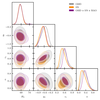
Figure 1: The 1-dimensional and 2-dimensional marginalized posterior distributions in the parameter space $(H_{0},q_{0},z_{t},\alpha)$ for the case when $q_{f}$ is free.

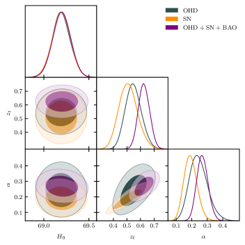
Figure 2: The 1-dimensional and 2-dimensional marginalized posterior distributions in the parameter space $(H_{0},z_{t},\alpha)$ for the case when $q_{f}=-1$.

In FIG. 2, we display 2D marginalized confidence level regions for parameter space $(H_{0},q_{0},z_{t},\alpha)$ using $OHD$, $SN$ and $OHD+SN+BAO$. Finally, we plot the deceleration parameter $q(z)$, the equation of state parameter $\omega(z)$, and the jerk parameter $j(z)$ for all these considered data in FIG. LABEL:fig2. The behavior of $q(z)$ shows a signature flip and $z_{t}$ indicates the epoch when the expansion of the universe went from a decelerating to an accelerating phase in the recent past. There is an uninspired phase of the universe when $z\rightarrow-1$ since $q(z)$ diverges more from the de-sitter phase for the combined dataset. Another choice for $q_{f}$ could also be made to ensure the model’s consistency in the distant future. Consequently, an additional analysis is required. The plot also displays the evolution of the equation of state parameter with respect to $z$. It reveals that the $\omega$ is positive at higher redshifts and remains greater than $-1$ (quintessence phase) until the present time for all the datasets but crosses a phantom divide for the far future. The present value of $\omega$ is $-0.72\pm 0.1$, $-0.78^{+0.09}_{-0.07}$, and $-0.76^{+0.08}_{-0.07}$ for $OHD$, $SN$, and $OHD+SN+BAO$, respectively.
However, the function $j(z)=q(2q+1)+(1+z)\frac{dq}{dz}$ demonstrates the deviation of $j$ from the flat $\Lambda$CDM model $(j=1)$ in the best-fit model. The jerk parameter is often used to discriminate against various dark energy models. Observations indicate that, in this model, the current value of $j$ exceeds 1 for all the datasets ($j_{0}=1.3$, $1.71$, $1.7$ for $OHD$, $SN$, $OHD+SN+BAO$, respectively) [36]. Therefore, based on the existing model (where $j\neq 1$ and $q_{0}<0$), it is evident that the dynamic dark energy model considered is the most probable explanation for the current acceleration and needs attention. But in this case, the $j(z)$ is not well constrained as it may be connected to the appearance of abrupt future singularities [34, 35].

IV.2 When $q_{f}$ is $-1$

Let us consider the case in which, besides fixing $q_{i}=1/2$, the final value of the deceleration parameter is fixed to the value $q_{f}=-1$, such that asymptotically in the future, i.e., $z=-1$, the model approaches to a de-sitter phase. Models such as $\Lambda$CDM, DGP, quintessence Chaplygin gas, etc., belong to this class of models [37]. By fixing $q_{f}$, we are left with only three free parameters, namely $(H_{0},z_{t},\alpha)$. We present the $68\%$ and $95\%$ confidence level for this parameter space in FIG. 2. The present values of $q$ for $OHD$, $SN$, and $OHD+SN+BAO$ are obtained explicitly using equation (6), as mentioned in Table 1.
We plot the deceleration parameter $q(z)$, equation of state parameter $\omega(z)$, and jerk parameter $j(z)$ for all these considered data in FIG. LABEL:fig4. The behavior of $q(z)$ shows a signature flip and $z_{t}$ indicates the epoch when the expansion of the universe went from a decelerating to an accelerating phase in the recent past and approaches a de-sitter phase as expected. The present values of $\omega$ are obtained as $-0.74^{+0.03}_{-0.06}$, $-0.81^{+0.02}_{-0.04}$, $-0.75^{+0.02}_{-0.03}$ for $OHD$, $SN$, $OHD+SN+BAO$, respectively. It reveals that the $\omega$ is positive at higher redshifts and remains greater than -1 (quintessence phase). It does not cross a phantom divide for the far future in this case.
For this mode, the jerk parameter $j(z)$ is found to be evolving, which indicates a tendency of deviation of the universe from the standard $\Lambda$CDM model. Observations indicate that, in this model, the current value of $j$ exceeds 1 for all the datasets ($j_{0}=1.3$, $1.51$, $1.2$ for $OHD$, $SN$, $OHD+SN+BAO$, respectively). Therefore, based on the existing model (where $j\neq 1$ ), it is evident that the present model seems to converge to 1, i.e., the standard $\Lambda$CDM in the near future. This would indicate that the higher value of $H_{0}$ leads to a lower jerk constraint and decreasing $z_{t}$. The significant deviations from the $\Lambda$CDM predictions suggest a preference for using a parametrization of the dynamical parameter for understanding the dark sector of the universe. It should be noted that the present values of $q_{0}$, $H_{0}$, $z_{t}$ are consistent with the values obtained by many authors [38, 39, 40] (also shown in figures LABEL:fig8 and 9).

IV.3 When $\alpha=1/3$

We also considered the case of $\Lambda$CDM, when $\alpha$ is also fixed, i.e. $\alpha=1/3$. The parameter space here reduces to $(H_{0},z_{t})$. We have obtained $q_{0}$ from the same equation (6), mentioned in Table 1. We present the $68\%$ and $95\%$ confidence levels for this parameter space in FIG. 5. It is clear that the $\Lambda$CDM is in good agreement with the data and used for comparing with the two previous cases. Here, the BAO measurements are giving us tighter constraints on the parameters. The behavior of $q(z)$ shows a signature flip and $z_{t}$ indicates the epoch when the expansion of the universe went from a decelerating to an accelerating phase in the recent past and approaches a de-sitter phase as expected. In this case, the jerk parameter is $j=1$ for the best-fit values, consistent with the observations.

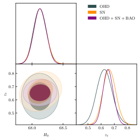
Figure 5: The 1-dimensional and 2-dimensional marginalized posterior distributions in the parameter space $(H_{0},z_{t})$ for the case when $\alpha=1/3$.

In FIG. 6, we have shown the evolution of the Hubble parameter $H(z)$ as a function of redshift $z$ compared with 31 $H(z)$ measurements. We have plotted the data points for $H(z)$ with $1\sigma$ error bars. We have observed that our model is well consistent with the $H(z)$ data against redshift for free $q_{f}$, $q_{f}=-1$, $\alpha=1/3$. For a convenient display, we also show $H(z)/(1+z)$ in FIG. 6.

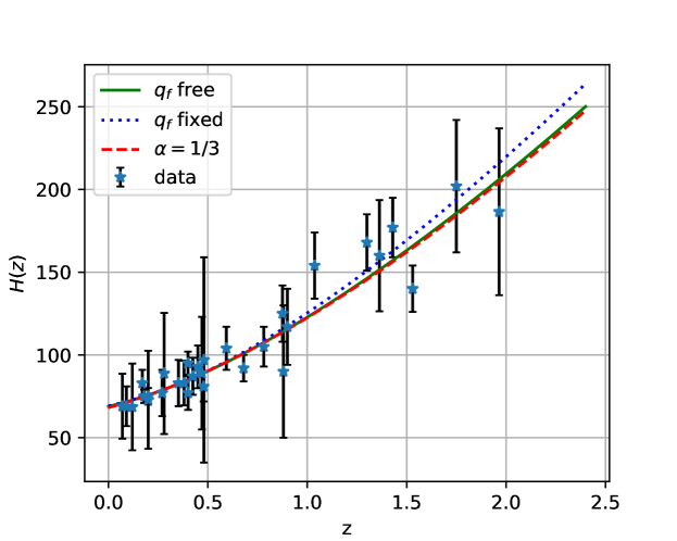
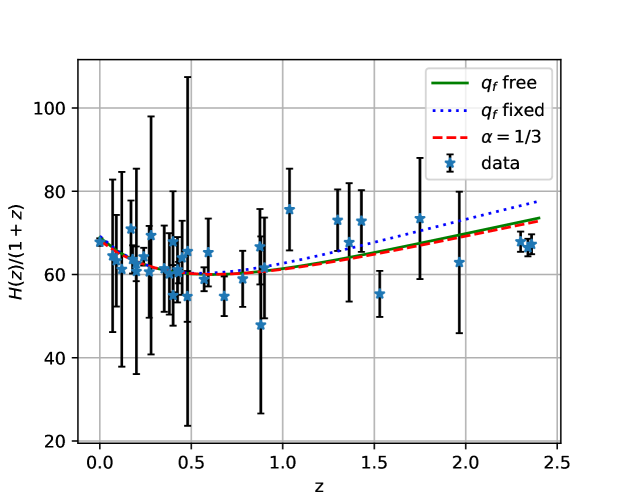
Figure 6: Figure shows the evolution of Hubble parameter $H(z)$ and $H(z)/(1+z)$ as a function of $z$. We have plotted 31 $H(z)$ measurements with its $1\sigma$ error bars for all the cases considered.

Model	Datasets	$H_{0}$	$q_{0}$	$z_{t}$	$\alpha$	$\chi_{\rm min}^{2}$	$\rm AIC$	$\rm BIC$
	OHD	$68.90\pm 0.24$	$-0.59^{+0.19}_{-0.15}$	$0.606^{+0.081}_{-0.13}$	$0.33^{+0.13}_{-0.19}$	$16.128$	$24.128$	$29.864$
$q_{f}$ is free	SN	$68.91\pm 0.25$	$-0.68^{+0.14}_{-0.11}$	$0.548^{+0.069}_{-0.13}$	$0.27^{+0.11}_{-0.22}$	$1043.385$	$1051.385$	$1071.203$
	OHD+SN+BAO	$68.93^{+0.23}_{-0.29}$	$-0.65^{+0.13}_{-0.11}$	$0.627^{+0.062}_{-0.085}$	$0.38^{+0.12}_{-0.16}$	$1062.084$	$1086.084$	$1110.805$
Model	Datasets	$H_{0}$	$q_{0}$	$z_{t}$	$\alpha$	$\chi_{\rm min}^{2}$	$\rm AIC$	$\rm BIC$
	OHD	$69.19\pm 0.10$	$-0.619^{+0.05}_{-0.10}$	$0.544^{+0.053}_{-0.063}$	$0.245^{+0.051}_{-0.065}$	$16.657$	$22.657$	$26.959$
$q_{f}=-1$	SN	$69.196\pm 0.098$	$-718^{+0.04}_{-0.06}$	$0.510^{+0.063}_{-0.074}$	$0.191^{+0.038}_{-0.044}$	$1044.081$	$1050.081$	$1064.945$
	OHD+SN+BAO	$69.199\pm 0.099$	$-0.629^{+0.03}_{-0.04}$	$0.626\pm 0.041$	$0.269^{+0.034}_{-0.038}$	$1064.676$	$1082.676$	$1101.217$
Model	Datasets	$H_{0}$	$q_{0}$	$z_{t}$	$\alpha$	$\chi_{\rm min}^{2}$	$\rm AIC$	$\rm BIC$
	OHD	$68.14\pm 0.11$	$-0.522^{+0.037}_{-0.034}$	$0.623\pm 0.060$	$1/3$	$18.193$	$22.193$	$25.061$
$\alpha$ fixed	SN	$68.13\pm 0.10$	$-0.545^{+0.027}_{-0.028}$	$0.663\pm 0.049$	$1/3$	$1044.981$	$1048.981$	$1058.89$
	OHD+SN+BAO	$68.129\pm 0.099$	$-0.54^{+0.022}_{-0.023}$	$0.654\pm 0.039$	$1/3$	$1066.039$	$1078.039$	$1090.4$

Table 1: Summary of the best-fit values of model parameters and statistical analysis using OHD, SN, and OHD+SN+BAO, including the 68% and 95% confidence levels.

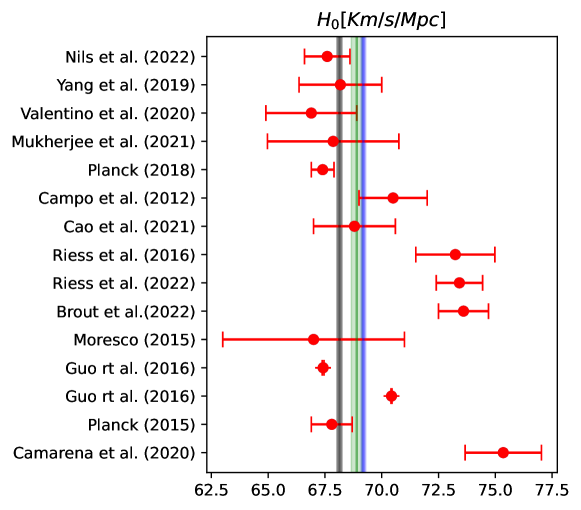
Figure 9: The plots represents the present values of $H_{0}$ with their corresponding error bars obtained from several works. The green, blue, and black lines represent the best-fit estimated values obtained for the current model in all three scenarios (free $q_{f}$, $q_{f}=-1$, $\alpha=1/3$), with the related $1\sigma$ error shown as shaded portions [40].

V Conclusion

In this work, we reexamined a kink-like parametrization for the deceleration parameter to investigate the transition from cosmic deceleration to acceleration in a spatially flat FLRW universe. The functional form of $q(z)$ involves $q_{f}$, $q_{i}$, $q_{0}$, $z_{t}$, $\alpha$, and $H_{0}$ as free parameters. Given that our parametrization specifically intends to explain the cosmic evolution that begins with a matter-dominated decelerated phase, we set the value of $q_{i}=1/2$. However, as new data pour in and new techniques evolve, revisiting the nature of $q$ with newer datasets is imperative. So, here, we focussed on recent OHD, SN (Pantheon samples), and BAO/CMB observations and carried out a Markov chain Monte Carlo (MCMC) analysis of the model, which allowed us to determine the optimal values of the model parameters.
We first consider the case in which we do not impose a fixed value for $q_{f}$. So, we constrained four parameters namely $(H_{0},q_{0},z_{t},\alpha)$. The comparison of the observational data on the OHD shows a good agreement with the $\Lambda$CDM model. The AIC analysis also substantiates the presence of a little tension for $OHD+SN+BAO$ between the current model for this scenario and the $\Lambda$CDM predictions. However, to definitively address this matter, additional observational evidence covering a more comprehensive range of redshifts is required. There is an uninspired phase of the universe when $z\rightarrow-1$ since $q(z)$ diverges more from the de-sitter phase for the combined dataset. Another choice for $q_{f}$ could also be made to ensure the model’s consistency in the distant future. The evolution of the equation of state parameter reveals that the $\omega$ is positive at higher redshifts and remains greater than $-1$ (quintessence phase) until the present time but crosses a phantom divide for the far future. The present value of $\omega$ is $-0.72$, $-0.78$, and $-0.76$ for $OHD$, $SN$, and $OHD+SN+BAO$, respectively. The current value of $j$ exceeds $1$ for all the datasets ($j_{0}=1.3$, $1.71$, $1.7$ for $OHD$, $SN$, $OHD+SN+BAO$, respectively). But in this case, the $j(z)$ is not well constrained as it may be connected to the appearance of abrupt future singularities.

We also examined the scenario where the model exhibits the final de-Sitter phase, characterized by $q_{f}=-1$. The Pantheon samples are the primary source for improvements compared to prior works. It is anticipated that these samples lead to a substantial enhancement in the constraints, owing to their higher statistics. By incorporating these datasets, we analyze the influence of $H_{0}$ on the transition $z_{t}$. We find that the cosmological deceleration-acceleration transition depends on the value of $H_{0}$ but is otherwise mildly dependent on other cosmological parameters. The Hubble parameter is not so far from the current bounds, agreeing with the Scolnic 2018 results [23]. Here, the jerk parameter is well constrained as it converges to $j_{0}=1$ at late times.
We also considered the case of $\Lambda$CDM, when $\alpha$ is also fixed, i.e. $\alpha=1/3$. The parameter space here reduces to $(H_{0},z_{t})$. The values of cosmological parameters, including the jerk parameter $j=1$, are consistent with the observations considered.
Our results have shown that the present model may represent an interesting alternative to dark energy for the case of $q_{f}=-1$ to tighten the constraints on the parameters for $OHD$, $Pantheon$, and $BAO$. Furthermore, it is worth noting the potential of future surveys such as DESI, LSST, SH0ES, and BINGO observations in effectively constraining the range of these model parameters.

Data Availability Statement

There are no new data associated with this article.

References

- [1] P.J. Steinhardt, Scientific American, 304, 36 (2011).
- [2] S. Weinberg, Rev. Mod. Phys., 61, 1 (1989).
- [3] P.J. Steinhardt et al., Phys. Rev. Lett., 59, 123504 (1999).
- [4] J. Yoo, Y. Watanabe, Int. J. Mod. Phys. D, 21, 1230002 (2012).
- [5] E. Di Valentino, A. Melchiorri, J. Silk, Nature Astronomy, 4, 196 (2020).
- [6] M. Benetti, S. Capozziello, J. Cosmol. Astropart. Phys., 2019 008 (2019).
- [7] A.G. Riess et al., Astron. J., 116, 1009 (1998).
- [8] S. Perlmutter et al., Astrophys. J., 517, 565 (1999).
- [9] E. Komatsu et al., Astrophys. J. Supp., 192, 18 (2011).
- [10] Planck Collaboration XVI, Astron. Astrophys., 571, A16 (2014).
- [11] W.J. Percival et al., Mon. Not. R. Astron. Soc. Lett., 381, 1053 (2007).
- [12] O. Farooq et al., Astrophys. J., 835, 26 (2017).
- [13] R. Nair, S. Jhingan, and D. Jain, J. Cosmol. Astropart. Phys., 01, 018 (2012).
- [14] A. Mukherjee, N. Banerjee, Class. Quantum Grav., 34 035016 (2017).
- [15] K. Asvesta et al., Mon. Not. R. Astron. Soc., 513, 2394-2406 (2002).
- [16] G.N. Gadbail et al., Chin. J. Phys., 79, 246-255 (2022).
- [17] S.K.J. Pacif, S. Arora, and P.K. Sahoo, Phys. Dark Univ., 32, 100804 (2021).
- [18] A.G. Riess et al., Astrophys. J., 607, 665 (2004).
- [19] L. Xu, W. Li, and J. Lu, J. Cosmol. Astropart. Phys., 07, 031 (2009).
- [20] E.E.O Ishida et al., Astropart. Phys., 28, 547 (2008); R. Giostri et al., J. Cosmol. Astropart. Phys., 03, 027 (2012); M. V. dos Santos, R.R.R. Reis, and I, Waga, J. Cosmol. Astropart. Phys., 02, 066 (2016).
- [21] D. F. Mackey et al., Publ. Astron. Soc. Pac., 125, 306 (2013).
- [22] H. Yu, B. Ratra, and F-Y Wang, Astrophys. J., 856, 3 (2018); M. Moresco, Mon. Not. R. Astron. Soc. Lett., 450, L16–L20 (2015).
- [23] D. M. Scolnic et al., Astrophys. J., 859, 101 (2018).
- [24] Z. Chang, D. Zhao, and Y. Zhou, Chin. Phys. C, 43, 125102 (2019).
- [25] R. Tripp, Astron. Astrophys., 331, 815-820 (1998).
- [26] R. Kessler and D. Scolnic, Astrophys.J., 836, 56 (2017).
- [27] H-K Deng and H. Wei, Eur. Phys. J. C, 78, 755 (2018).
- [28] N. Aghanim et al., A & A, 594, A13 (2016).
- [29] D. J. Eisenstein et al., Astrophys. J., 633, 560-574, (2005).
- [30] R. Giostri et al., J. Cosmol. Astropart. Phys., 2012, 027 (2012).
- [31] C. Blake et al., Mon. Not. R. Astron. Soc., 418, 1707-1724 (2011).
- [32] H. Akaike, IEEE Transactions on Automatic Control, 19, 716-723 (1974).
- [33] A. R. Liddle, Mon. Not. R. Astron. Soc. Lett., 377, L74-L78 (2007).
- [34] M. P. Dabrowski, Phys. Lett. B, 625, 184-188 (2005).
- [35] S. Pan et al., Mon. Not. R. Astron. Soc., 477, 1189-1205 (2018).
- [36] A. Al Mamon and K. Bamba, Eur. Phys. J. C, 78, 862 (2018).
- [37] G. Dvali, G. Gabadadze, and M. Porrati, Phys. Lett. B, 485, 208 (2000); N. Bilic, G.B. Tupper, and R.D. Viollier, Phys. Lett. B, 535, 17 (2002); M. Bento, O. Bertolami, and A. Sen, Phys. Rev. D, 66, 043507 (2002); Y. Wang et al., Astrophys. J, 594, 25 (2003); G. N. Gadbail, S. Arora, and P.K. Sahoo, Ann. Phys., 451, 169269 (2023); G. N. Gadbail, S. Arora, and P.K. Sahoo, Phys. Dark Univ., 37, 101074 (2022).
- [38] S. Capozziello, Peter K.S. Dunsby, O. Luongo, Mon. Not. R. Astron. Soc., 509, 5399-5415 (2022).
- [39] P. Mukherjee and N. Banerjee, Eur. Phys. J. C, 81, 36 (2021); P. Mukherjee and N. Banerjee, Phys. Dark Univ., 36, 100998 (2022); S. del Campo et al., Phys. Rev. D, 86, 083509 (2012); A. Al Mamon and K. Bamba, Eur. Phys. J. C, 78, 862 (2018); A. Al Mamon and S. Das, Int. J. Mod. Phys. D, 25, 1650032 (2016); A. Al Mamon, Mod. Phys. Lett. A, 33, 1850056 (2018); L. Xu, W. Li, and J. Lu, J. Cosmol. Astropart. Phys., 07, 031 (2009); H. Chaudhary et al., Gen. Relativ. Gravit., 55, 133 (2023); H. Chaudhary et al., Phys. Scr., 98, 095006 (2023); A. Al Mamon and S. Das, Eur. Phys. J. C, 77, 495 (2017); D. Camarena and V. Marra, Phys. Rev. Research, 2, 013028 (2020); S. Kumar, Mon. Not. R. Astron. Soc., 42, 2532-2538 (2012); L. Xu et al., Mod. Phys. Lett. A, 23, 1939-1948 (2008); S. Rani et al., J. Cosmol. Astropart. Phys.,03, 031 (2015).
- [40] P. A. R. Ade et al., A & A, 594, A13 (2016); E. Di Valentino et al., J. Cosmol. Astropart. Phys.,01, 013 (2020); W. Yang et al., Mon. Not. R. Astron. Soc., 490, 2071-2085 (2019); N. Schoneberg et al., J. Cosmol. Astropart. Phys., 11, 039 (2022); D. Brout et al., Astrophys. J., 938, 110 (2022); A. G. Riess et al., Astrophys. J. Lett., 934, L7 (2022); A. G. Riess et al., Astrophys. J., 826, 56 (2016); R-Y Guo and X. Zhang, Eur. Phys. J. C, 76, 163 (2016); S. Cao, J. Ryan, and B. Ratra, Mon. Not. R. Astron. Soc., 504, 300-310 (2021); M. Moresco, Mon. Not. R. Astron. Soc., 450, L16-L20 (2015); N. Aghanim et al., A & A, 64, A6 (2020).