Point Transformer with Federated Learning for Predicting Breast Cancer HER2 Status from Hematoxylin and Eosin-Stained Whole Slide Images

Abstract

Directly predicting human epidermal growth factor receptor 2 (HER2) status from widely available hematoxylin and eosin (HE)-stained whole slide images (WSIs) can reduce technical costs and expedite treatment selection. Accurately predicting HER2 requires large collections of multi-site WSIs. Federated learning enables collaborative training of these WSIs without gigabyte-size WSIs transportation and data privacy concerns. However, federated learning encounters challenges in addressing label imbalance in multi-site WSIs from the real world. Moreover, existing WSI classification methods cannot simultaneously exploit local context information and long-range dependencies in the site-end feature representation of federated learning. To address these issues, we present a point transformer with federated learning for multi-site HER2 status prediction from HE-stained WSIs. Our approach incorporates two novel designs. We propose a dynamic label distribution strategy and an auxiliary classifier, which helps to establish a well-initialized model and mitigate label distribution variations across sites. Additionally, we propose a farthest cosine sampling based on cosine distance. It can sample the most distinctive features and capture the long-range dependencies. Extensive experiments and analysis show that our method achieves state-of-the-art performance at four sites with a total of 2687 WSIs. Furthermore, we demonstrate that our model can generalize to two unseen sites with 229 WSIs. Code is available at: https://github.com/boyden/PointTransformerFL

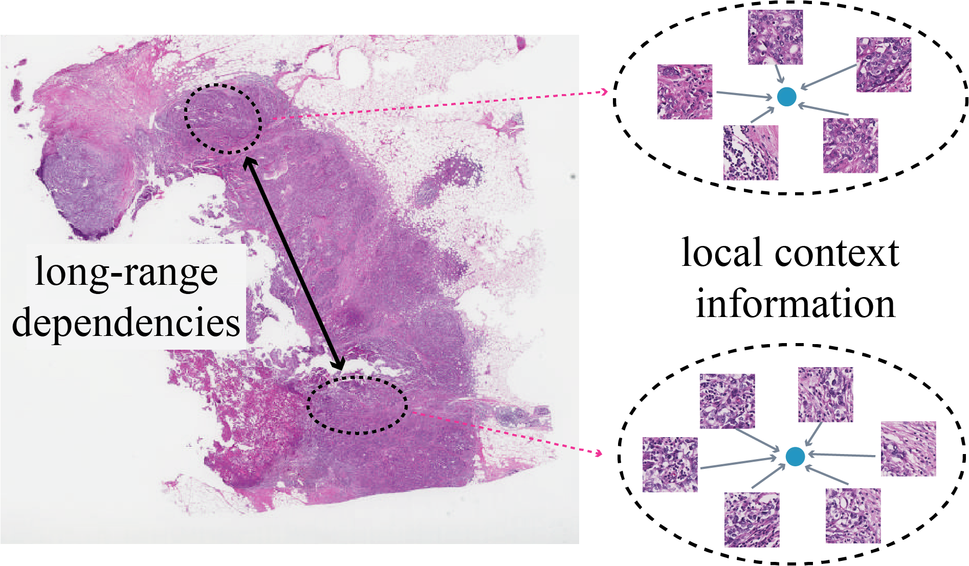
Figure 1: Local context information and long-range dependencies are both essential for WSI analysis

Introduction

Hematoxylin and eosin (HE)-stained whole slide images (WSIs) are now being used beyond visible tasks by applying deep learning methods (Lu et al. 2021; Shao et al. 2021; Li et al. 2022). These images contain subtle molecular characteristics that can be inferred using deep learning (Kather et al. 2020; Farahmand et al. 2022; Lu et al. 2022c). In breast cancer, accurately predicting human epidermal growth factor receptor 2 (HER2) status is crucial for guiding anti-HER2 treatment decisions  (Oh and Bang 2019). Routinely, pathologists rely on HE-stained WSIs for breast cancer diagnosis, followed by specialized immunohistochemistry (IHC) and/or costly in-situ hybridization (ISH) techniques (Wolff et al. 2018) to determine HER2 status. By utilizing deep learning, we can predict HER2 status from broadly accessible HE-stained WSIs without requiring IHC and/or ISH.

Achieving better WSI-level prediction requires large amounts of WSIs. Federated learning (FL) (McMahan et al. 2017) has already exhibited promising progress in WSI analysis (Lu et al. 2022b; Jiang, Wang, and Dou 2022; Ogier du Terrail et al. 2023). It can incorporate a large amount of multi-site WSIs without actual transportation of gigabyte-size WSIs and reduce the risk of data leakage. However, real-world WSIs exist non-independent and identically distributed (non-i.i.d.) scenarios. For HER2 classification, labeling imbalance and varying histological specimen preparation at different sites can adversely affect the overall performance. Although many studies have addressed the non-i.i.d. challenges (Hu et al. 2022; Guan and Liu 2023; Zhuang and Lyu 2023) in natural scenes, these methods remain a major gap in real-world WSIs compared to centralized learning.

In the site-end feature representation, WSIs are cut into patches, and these patches’ local context information and long-range dependencies (as shown in Figure 1) are essential for WSI-level prediction, such as HER2 prediction  (Kather et al. 2020; Lu et al. 2022c) and survival analysis (Chen et al. 2021b; Shen et al. 2022; Shao et al. 2023). For HER2 prediction, HER2-positive patches may cluster in many separate regions of WSIs. Existing deep learning methods either treat these patches as instances using multi-instance learning (MIL) methods  (Lu et al. 2021; Shao et al. 2021, 2023), or structure the patches into a graph using graph neural networks (GNNs) (Chen et al. 2021a; Lu et al. 2022c; Hou et al. 2022). However, the MIL-based methods lack the ability to model the local contextual information while the graph-based methods may struggle to capture long-distance dependence (Xu et al. 2018) and need extra edge representation. Alternatively, the point neural network (Qi et al. 2017a, b) can treat each patch as a point with inherent position information in the Euclidean space, and hence effectively model the local context by considering the position information. Moreover, it is permutation invariant and has demonstrated proficiency in aggregating features and representing long-range dependencies (Guo et al. 2021; Lu et al. 2022a), making it well-suited for WSI analysis.

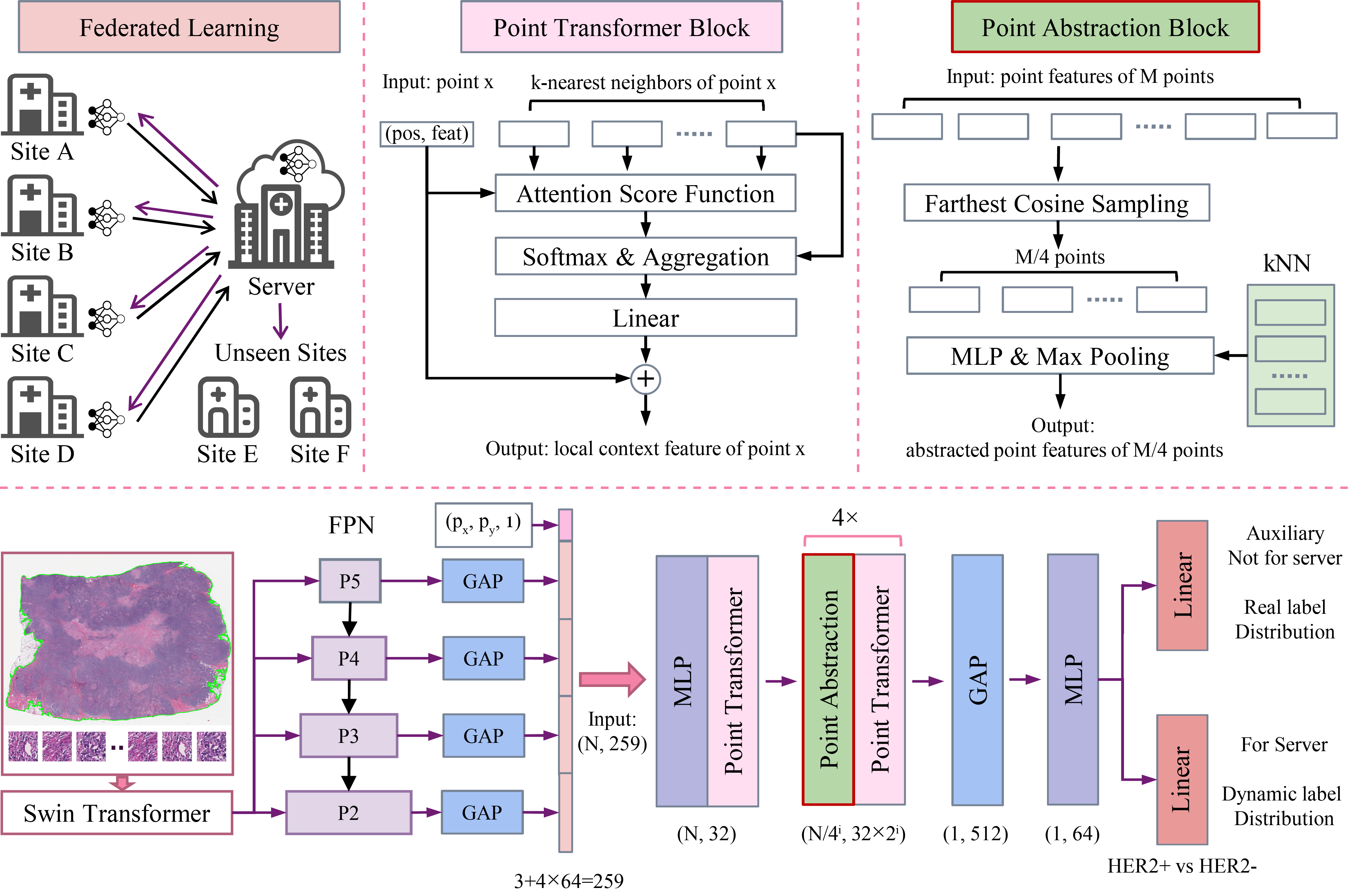
Figure 2: Overview of the point transformer for predicting HER2 status from whole slide images in a federated learning framework. 4$\times$ represents that the corresponding blocks are repeated 4 times. In the $i_{th}$ block, the output shape of point features is $(N/4^{i},32\times 2^{i})$ and $N$ represents the total point numbers and is set to 1024. FPN: feature pyramid network, GAP: global average pooling, MLP: multilayer perceptron.

In this paper, we introduce a PointTransformerDDA+ to represent both the local context and the long-range dependencies. Through the point transformer block, it can capture and aggregate the local information by employing attention mechanisms enriched with position information. We also propose a novel Farthest Cosine Sampling (FCS) to capture the long-range dependencies and gather the most distinctive features based on their cosine distance. To mitigate federated learning’s label-imbalance of multi-site, we present a dynamic distribution adjustment (DDA) method for a well-initialized model. It includes a distribution adjustment strategy and an auxiliary classifier. The DDA allows the resampling of labels to the same imbalance ratio initially and then dynamically adjust to the real imbalance ratio for each site without degrading the feature representation.

Our main contributions can be summarized as follows:

• Unlike MIL models or graph models, we pioneer the use of point transformer for WSI analysis, which effectively captures both local context and long-range dependencies.

• Our proposed FCS can capture the long-range dependencies, leading to the most distinct feature aggregation.

• The proposed DDA mitigates the multi-site class imbalance issue, thereby enhancing model generalization.

• Extensive experiments on the largest WSI dataset to date for HER2 prediction in breast cancer demonstrate that our method achieves state-of-the-art performance in four sites (2687 WSIs) and two unseen sites (229 WSIs).

Related Work

In this section, we briefly review relevant works on WSI classification and federated learning in WSI analysis.

Whole Slide Image Classification

Recent works have used either MIL-based or graph-based methods for WSI classification, including molecular biomarkers such as HER2 status prediction (Farahmand et al. 2022; Lu et al. 2022c). The MIL-based methods commonly leverage attention mechanisms (Ilse, Tomczak, and Welling 2018; Chen et al. 2020; Lu et al. 2021) or transformers (Shao et al. 2021; Shen et al. 2022) to capture the long-distance dependence among instances. Regarding the local spatial relationship, DSMIL (Li, Li, and Eliceiri 2020) simply extracts feature from different scales and concatenate them among scales, which do not consider the local information in a specific scale. TransMIL (Shao et al. 2021) models the spatial relationship among patches via transformers with conditional position encoding; however, the positions used are not based on the actual Euclidean space. Graph-based models (Hamilton, Ying, and Leskovec 2017; Xu et al. 2019; Lee et al. 2022) are intrinsically designed to capture local information by a graph structure. In WSI analysis, Patch-GCN (Chen et al. 2021a) regards patches as 2D point clouds while still employing GNN to analyze WSIs. SlideGraph+ (Lu et al. 2022c) also constructs a graph based on position information and uses edge convolution (Wang et al. 2019) to model local neighbor features, leading to a SOTA HER2 prediction performance. However, the long-term dependency may limit the further improvement of GNNs in WSI analysis. While the permutation-invariant point neural network (Qi et al. 2017b; Zhao et al. 2021; Lu et al. 2022a) can capture both the local context and long-range dependencies, few studies have focused on WSI classification.

Federated Learning in WSI Analysis

Federated learning (McMahan et al. 2017; Guan and Liu 2023) can facilitate the training of data-driven models using multi-site WSIs. HistFL (Lu et al. 2022b) collaborates multi-sites WSI with attention MIL model and differential privacy for cancer subtype and survival prediction. Also, TNBC-FL (Ogier du Terrail et al. 2023) employs federated learning for predicting treatment outcomes in the rare subtype of breast cancer. However, general non-i.i.d. issues like skewed label distribution impedes the performance of federated learning. In natural scenes, several works replace batch normalization with group normalization (Hsieh et al. 2020), layer normalization (Du et al. 2022) or even remove the normalization layer (Zhuang and Lyu 2023) to address the problems by reducing the external covariate shift. FedProx (Li et al. 2020) introduces a regularization function to guarantee robust convergence of model in non-i.i.d. data. Additionally, FedMGDA (Hu et al. 2022) regards multi-site federated learning as a multi-objective optimization problem, aiming to converge to Pareto stationary solutions. With gradient normalization named FedMGDA+ (Hu et al. 2022), it can increase the model’s robustness. Despite the progress made in federated learning, there still remains a gap between federated learning and centralized learning in real WSIs and further improvements are still needed.

Methodology

In this section, we start by introducing the problem definition of HER2 status prediction using a point transformer with federated learning. Then we describe the main components of the framework, including point feature extraction, point transformer block, point abstraction block, and federated learning with dynamic distribution adjustment. Figure 2 illustrates the overall pipeline of our proposed framework.

Preliminaries

Suppose that we have $M$ sites for HER2 status prediction, our goal is to accurately determine whether a given Whole Slide Image (WSI) is HER2-positive (HER2+) or HER2-negative (HER2-). For the $i_{th}$ site, it contains a labeled point dataset $\mathcal{P}_{i}=\{(\mathcal{X}_{n},y_{n})\mid n\in(1,...,|\mathcal{P}_{i}|)\}$, where $y_{n}\in\{0,1\}$ is the corresponding HER2- and HER2+ status. Within this dataset, $\mathcal{X}_{n}=\{x_{n,1},x_{n,2},...,x_{n,|\mathcal{X}_{n}|}\}$ represents a point set in the $n_{th}$ whole slide images, where a point $x_{n,k}\in\mathbb{R}^{3+d}$ is a feature vector with 3-dim coordinates and $d$-dim point features. To determine HER2+ status from a point set $\mathcal{X}$ while considering data privacy, we employ federated learning to minimize the global cost over all sites:

$$\mathop{\arg\min}_{\mathbf{W}}\mathcal{L}(\mathbf{W}) =\sum_{i=1}^{M}\frac{|\mathcal{P}_{i}|}{|\mathcal{P}|}\mathcal{L}_{i}(\mathcal{P}_{i};\mathbf{W}),$$ (1)

where $|\mathcal{P}|=\sum_{i=1}^{M}|\mathcal{P}_{i}|$ is the total number of WSIs across all sites. For the $i_{th}$ site, the cost can be calculated by:

$$\mathcal{L}_{i}(\mathcal{P}_{i};\mathbf{W}) =\frac{1}{|\mathcal{P}_{i}|}\sum_{(\mathcal{X}_{k},y_{k})\in\mathcal{P}_{i}}\ell(f_{c}(f_{h}(\mathcal{X}_{k})),y_{k};\mathbf{W}),$$ (2)

where $\ell$ is the loss function, $f_{h}:\mathcal{X}\mapsto\mathbb{R}^{d}$ is a point set embedding function, and $f_{c}:\mathcal{R}^{d}\mapsto\mathbb{R}$ is the final classifier function. WSIs from real sites have a general non-independent and identically distributed (non-i.i.d. ) scenario where each site has different HER2 status distributions. For the $i_{th}$ site, we denote the class imbalance ratio as $\gamma_{i}=\frac{|\mathcal{P}_{i}^{-}|}{|\mathcal{P}_{i}^{+}|}$, where $|\mathcal{P}_{i}^{-}|$ and $|\mathcal{P}_{i}^{+}|$ represent to the number of HER2- and HER2+ WSIs within the $i_{th}$ site.

Point Feature Extraction

To extract point features from a WSI, we follow the CLAM (Lu et al. 2021) to preprocess and patch the WSIs with details in Appendix A. Each patch is treated as a point. The corresponding coordinates for each patch are also traced and represented as a tuple$(p_{x},p_{y},1)$, where 1 represents all WSIs having the same z-coordinate. Then we input the patches into a nuclei segmentation network that is pretrained using Swin-Transformer (Liu et al. 2021) with FPN (Lin et al. 2017) with four levels, represented by ${P_{2},P_{3},P_{4},P_{5}}$ in Figure 2. The channel of FPN is set to 64 and the outputs from all four layers of FPN are averaged and concatenated with the point coordinates as the patch-level feature $x_{n}\in\mathbb{R}^{3+d}$, where 3 represents the coordinates and $d=256$ represents the point feature. Thus for a WSI with a label $y$, we can obtain a point set $\mathcal{X}={x_{1},x_{2},...,x_{|\mathcal{X}|}}$, where $|\mathcal{X}|$ is the number of patches in a WSI. 1024 patches or points are randomly selected with uniform distribution to reduce the memory usage and improve computational efficiency.

Point Transformer Block

In our approach, we adopt the original point transformer block (Zhao et al. 2021) to capture and aggregate the local context information of each point with an effective attention mechanism. For the $i_{th}$ point with its corresponding point feature $x_{i}$, position $p_{i}$. We represent its k-nearest neighborhood points (k=16) as a subset $\mathcal{X}(i)\subset\mathcal{X}$. Then we compute the attention score between point $x_{i}$ and point subset $\mathcal{X}(i)$ by the attention score function $\alpha$:

$$\alpha(x_{i},x_{j})=W_{q}(W_{i}x_{i}-W_{j}x_{j})+PE(p_{i},p_{j}),$$ (3)

where $x_{j}\in\mathcal{X}(i)$ and $PE$ is a relative position encoding function defined as:

$$PE(p_{i},p_{j})=MLP(p_{i}-p_{j}).$$ (4)

MLP in the formula represents two linear layers with a ReLU activation function.

Afterward, we aggregate the localized feature around of point $x_{i}$ and obtain the aggregated feature $z_{i}$ with a softmax function $S$. Then the output $y_{i}$ is computed by applying a residual connection between $x_{i}$ and $z_{i}$:

$$z_{i}=\sum_{x_{j}\in\mathcal{X}(i)}S(\alpha(x_{i},x_{j})) \cdot(W_{v}x_{j}+PE(p_{i},p_{j})),$$ (5)

$$y_{i}=x_{i} +W_{z}z_{i}.$$ (6)

Point Abstraction Block

To effectively reduce the cardinality of a point set and capture the long-range dependencies without missing important points, we propose a novel sampling strategy named farthest cosine sampling (FCS), as an alternative to the farthest point sampling (FPS)  (Qi et al. 2017b).

In scenarios where a WSI exhibits a majority of negative patches with only a few positive patches clustered together in a specific region, FPS may miss these positive patches, as depicted in Figure 3. Consequently, it can lead to false negative predictions of HER2 status. Contrary to FPS, we perform sampling in the feature space, not in the position space. For a point set $\mathcal{X}_{1}=\{x_{1},x_{2},...,x_{M}\}$ with M points, we define the cosine distance as the distance metric between two points $x_{i},x_{j}\in\mathcal{X}_{1}$:

$$Dist(x_{i},x_{j})=1-\frac{x_{i}\cdot x_{j}}{\max(||x_{i}||_{2}\cdot||x_{j}||_{2},1e-8)}.$$ (7)

Algorithm 1 Farthest cosine sampling

Input: M points with feature $\mathcal{X}_{1}=\{x_{1},x_{2},...,x_{M}\}$.
Output: Sampled M/4 points $\mathcal{X}_{2}$.

1:  initialize an empty sampling point set $\mathcal{X}_{2}=\{\}$;

2:  $x_{s,1}$ = RandomChoiceOne($\mathcal{X}_{1}$);

3:  $\mathcal{X}_{1}\leftarrow\mathcal{X}_{1}\setminus\{x_{s,1}\};\mathcal{X}_{2}\leftarrow\{x_{s,1}\}$;

4:  while $|\mathcal{X}_{2}|<M/4$ do

5:     // Using cosine similarity for distance metric

6:     $Dist(i,j)$ = $1-\frac{x_{i}\cdot x_{s,j}}{\max(||x_{i}||_{2}\cdot||x_{s,j}||_{2},1e-8)}$;

7:     $\mathcal{D}=\{Dist(i,j);x_{i}\in\mathcal{X}_{1},x_{s,j}\in\mathcal{X}_{2}\}$;

8:     $x_{s}\leftarrow\mathop{\arg\max}_{x_{i}\in\mathcal{X}_{1}}(\mathcal{D})$;

9:     $\mathcal{X}_{1}\leftarrow\mathcal{X}_{1}\setminus\{x_{s}\};\mathcal{X}_{2}\leftarrow\mathcal{X}_{2}\cup\{x_{s}\}$;

10:  end while

11:  return $\mathcal{X}_{2}$

Using this distance metric, we iteratively select the $M/4$ farthest points based on Algorithm 1. Consequently, the FCS can effectively cover the most requisite patches and capture the long-range dependencies in the feature space for better prediction of HER2 status.

After FCS, we obtain a sampled point subset $\mathcal{X}_{2}=\{x_{s,1},x_{s,2},...,x_{s,M/4}\}$. For each sampled point $x_{i}\in\mathcal{X}_{2}$, we define its k-nearest neighborhood points (k=16) on $\mathcal{X}_{1}$ as a point subset: $\mathcal{X}_{2}(i)\subset\mathcal{X}_{1}$. Subsequently, we group the feature from $\mathcal{X}_{1}$ onto $\mathcal{X}_{2}$ as $y_{i}$ for each point $x_{i}\in\mathcal{X}_{2}$ using the following equation:

$$y_{i}=MaxPooling_{x_{j}\in\mathcal{X}_{2}(i)}(MLP(x_{j})).$$ (8)

The MLP has two layers with each layer containing a linear transformation, batch normalization, and a ReLU activate function.

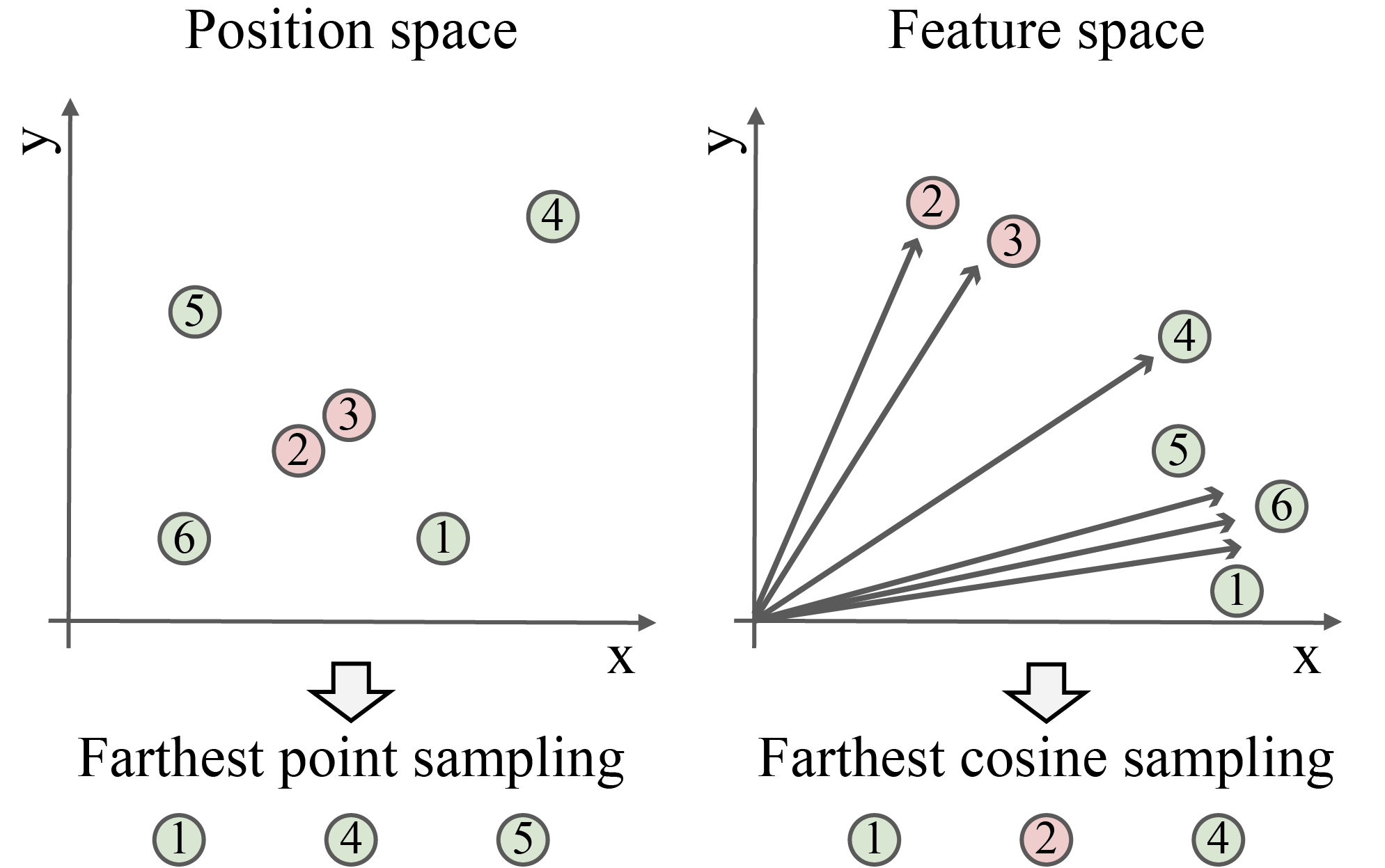
Figure 3: Difference between farthest point sampling and farthest cosine sampling. Light red: HER2+ points, light green: HER2- points.

Point Classifier Block

After performing $4\times$ attention and abstraction operations, we obtain 4 abstract points with a grouped feature representation denoted as $F_{g}\in\mathbb{R}^{4\times 512}$. By averaging the grouped feature, we derive the final WSI-level feature represented as $F_{h}\in\mathbb{R}^{64}$:

$$F_{h}=MLP(GAP(F_{g}))=f_{h}(\mathcal{X}),$$ (9)

where MLP has two layers with each layer containing a linear transformation and a ReLU activation function. Following the MLP, a linear layer with a softmax function named $f_{c}$ outputs the final HER2 status probabilities $p$. The loss is calculated using cross entropy (CE) loss function, which is formulated as:

$$\ell(p,y)=-\frac{1}{|\mathcal{P}|}\sum_{i}^{|\mathcal{P}|}\sum_{c=0}^{1}y_{c}^{i}\log(p_{c}^{i}).$$ (10)

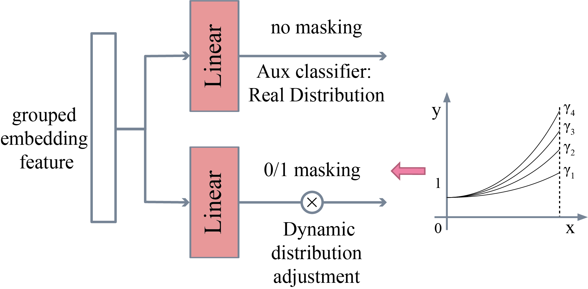
Figure 4: Dynamic distribution adjustment and auxiliary classifier for federated learning.

Federated Learning with Dynamic Distribution Adjustment

The WSIs from real sites exhibit a general non-independent and identically distributed (non-i.i.d.) scenario in which each site has different label distribution, which can impact the performance of federated learning (Guan and Liu 2023). To mitigate this issue, we introduce a novel dynamic distribution adjustment strategy. It subsampling the majority of HER2- WSIs to the same label distribution in the initial training stage of federated learning. Then the balanced label distribution dynamically adjusts to the real distribution after progressive training. Specifically, we keep all the HER2+ WSIs and generated a 0/1 mask $M(k)$ for the HER2- WSIs. This mask is created using a Bernoulli distribution $\mathcal{B}$ with a probability of $b_{k}$ at $k_{th}$ iteration.

$$M_{i}(k) =\mathcal{B}(b_{i}^{k}),$$ (11)

$$b_{i}^{k} =\frac{1}{\gamma_{i}}+(1-\frac{1}{\gamma_{i}})\cdot\frac{e^{k/K}-1}{e-1}\in[\frac{1}{\gamma_{i}},1],$$ (12)

where $\gamma_{i}$ is the $i_{th}$ site’s imbalanced ratio and $K$ is the total optimization steps. The loss function can be formulated as:

$$\mathcal{L}_{cls} =M\cdot\ell(f_{c}(F_{h}),y)$$ (13)

$$=-\frac{1}{|\mathcal{P}_{i}|}[\sum_{i}^{|\mathcal{P}_{i}^{-}|}M_{i}(k)\log(p_{0}^{i})+\sum_{i}^{|\mathcal{P}_{i}^{+}|}\log(p_{1}^{i})],$$ (14)

where $|P_{i}^{-}|,|P_{i}^{+}|$ represent the number of HER2- and HER2+ WSIs.

In every iteration $k$, we note $b_{i}^{k}\gamma_{i}$ as the imbalance ratio involved in loss computation. Figure 4 shows that at iteration $k=0$, all sites have $b_{i}^{k}\gamma_{i}=1$ indicating that they share the same label distribution with an equal ratio between HER2- and HER2+. As the training progresses, the distribution gradually shifts towards each site’s real distribution $\gamma_{i}$. By this strategy, the models are initially trained within a similar distribution, leading to a well-initialized model for accurately predicting HER2 status.

The above subsampling may arise a potential information loss problem, leading to insufficient feature representation. To address this concern, we add an auxiliary classifier that incorporates each site’s real label distribution:

$$\mathcal{L}_{aux}(p,y)=-\frac{1}{|\mathcal{P}_{i}|}[\sum_{i}^{|\mathcal{P}_{i}^{-}|} \log(p_{0}^{i})+\sum_{i}^{|\mathcal{P}_{i}^{+}|}\log(p_{1}^{i})],$$ (15)

$$\mathcal{L}_{total} =\mathcal{L}_{cls}+\mathcal{L}_{aux}.$$ (16)

This auxiliary classifier does not involved in the weights synchronization with the server model during the training of federated learning. Instead, it serves to guarantee the quality of feature representation as previous studies have demonstrated that models trained on imbalanced data can still learn high-quality feature representations (Kang et al. 2020; Lee, Shin, and Kim 2021). Detailed pseudo codes are shown in algorithm 2.

Experiments

Dataset and Experimental Settings

We evaluate our point transformer model for breast cancer HER2 status prediction using the largest WSI from six sites with a total of 2,916 WSIs. The sites are denoted as follows: Site A (TCGA-BRCA) (Network 2012), Sites B and C (internal hospitals with ethics committee approval), Site D (Conde-Sousa et al. 2022), and Sites E and F (Farahmand et al. 2022; Qaiser et al. 2017). Four sites participate in federated learning, while the remaining two sites serve as unseen data for external tests. Sites A, B, C, and D are split into training, validation, and test sets with a ratio of 6:1:3, as shown in Table 1. The splits are repeated five times, and the best model is selected based on the validation set in each split. The mean area under the ROC curve (AUC) is reported for the test set.

We refer to the point transformer with FCS as PointTransformer+, the variant with DDA as PointTransformerDDA, and the combined variant as PointTransformerDDA+.

WSIs	Federated Sites					Unseen Sites
	Site A	Site B	Site C	Site D	Total	Site E	Site F
HER2$-$	669	672	332	306	1979	98	26
HER2$+$	118	214	172	204	708	93	12
Total	787	886	504	510	2687	191	38
$\gamma$	5.7	3.1	1.9	1.5	2.8	1.1	2.2
Train	472	532	302	306	1612	-	-
Val	79	88	50	51	268	-	-
Test	236	266	152	153	807	191	38

Table 1: WSIs and their HER2 status number in each site. $\gamma_{i}=\frac{|\mathcal{P}_{i}^{-}|}{|\mathcal{P}_{i}^{+}|}$ represents the imbalance ratio. WSIs are split into training (60%), validation (10%), and test (30%) set.

Experiment	Method	Average	Site A	Site B	Site C	Site D
Ours	PointTransformerDDA+	0.816 ± 0.019	0.766 ± 0.025	0.866 ± 0.021	0.837 ± 0.036	0.760 ± 0.046
	PointTransformerDDA	0.793 ± 0.013	0.730 ± 0.029	0.855 ± 0.013	0.804 ± 0.024	0.758 ± 0.022
	PointTransformer+	0.806 ± 0.015	0.752 ± 0.018	0.844 ± 0.008	0.823 ± 0.024	0.757 ± 0.043
Point-based	PointTransformer [1]	0.771 ± 0.012	0.717 ± 0.037	0.834 ± 0.026	0.776 ± 0.037	0.721 ± 0.035
	PointNet++ [2]	0.763 ± 0.017	0.696 ± 0.039	0.830 ± 0.033	0.746 ± 0.045	0.730 ± 0.042
MIL-based	CLAM-SB [3]	0.767 ± 0.032	0.712 ± 0.044	0.793 ± 0.037	0.766 ± 0.072	0.748 ± 0.022
	DSMIL [4]	0.693 ± 0.096	0.647 ± 0.065	0.738 ± 0.103	0.706 ± 0.080	0.675 ± 0.111
	TransMIL [5]	0.790 ± 0.019	0.739 ± 0.038	0.824 ± 0.021	0.805 ± 0.036	0.759 ± 0.040
	HistoFL [6]	0.757 ± 0.039	0.729 ± 0.048	0.776 ± 0.050	0.759 ± 0.076	0.733 ± 0.012
Graph-based	GraphSAGE [7]	0.711 ± 0.026	0.656 ± 0.053	0.735 ± 0.027	0.692 ± 0.044	0.685 ± 0.021
	Patch-GCN [8]	0.750 ± 0.037	0.700 ± 0.035	0.768 ± 0.062	0.766 ± 0.030	0.727 ± 0.047
	SlideGraph+ [9]	0.783 ± 0.019	0.736 ± 0.029	0.828 ± 0.012	0.804 ± 0.037	0.785 ± 0.013

Table 2: Comparison of our model with other point, multi-instance, and graph-based models. [1] (Zhao et al. 2021), [2] (Qi et al. 2017b), [3] (Lu et al. 2021), [4] (Li, Li, and Eliceiri 2020), [5] (Shao et al. 2021), [6] (Lu et al. 2022b), [7] (Hamilton, Ying, and Leskovec 2017), [8] (Chen et al. 2021a), [9] (Lu et al. 2022c).

Algorithm 2 Point transformer with federated learning

Input: M participating sites with point set $\mathcal{P}_{m}=(\mathcal{X}_{m},y_{m})$
and label imbalanced ratio $\gamma_{m}$ where $m\in\{1,...,M\}$. Optimization epochs: K, communication pace: E.
Output: Model’s weights $W_{s}$.

1:  initialize the point transformer’s function: $f_{h},f_{c},f_{aux}$;

2:  initialize the same weights for the server and sites: $W_{s}^{0},W_{s,1}^{0},...,W_{s,M}^{0}$;

3:  for $k=0$ to $K-1$ do

4:     for $m=1$ to $M$ do

5:        $F_{h}=f_{h}(\mathcal{X}_{m})$;

6:        // Dynamic distribution adjustment

7:        $M_{m}=\mathcal{B}(\frac{1}{\gamma_{m}}+(1-\frac{1}{\gamma_{m}})\cdot\frac{e^{k/K}-1}{e-1})$;

8:        $\mathcal{L}_{m}=M_{m}\cdot\ell(f_{c}(F_{h}),y_{m})+\ell(f_{aux}(F_{h}),y_{m})$;

9:        // Local site update

10:        $W_{s,m}^{k+1}\leftarrow W_{s,m}^{k}-lr\cdot\nabla_{W_{s,m}^{k}}\mathcal{L}_{m}$;

11:     end for

12:     if $(k+1)\mod E=0$ then

13:        // Server site update

14:        for each layer $l$ in point transformer do

15:           if $l$ is not the auxiliary classifier’s layer then

16:              $W_{s}^{k+1,l}\leftarrow\sum_{m=1}^{M}{\frac{|\mathcal{P}_{i}|}{|\mathcal{P}|}W_{s,m}^{k+1,l}}$;

17:              $W_{s,m}^{k+1,l}\leftarrow W_{s}^{k+1,l}$;

18:           end if

19:        end for

20:     end if

21:  end for

22:  return $W_{s}$

Implementation Details

Our models are implemented using PyTorch 1.12.0 on a workstation with an RTX 3090 GPU. The models are trained for 200 epochs with a learning rate of 1e-3 and L2 regularization of 1e-5. Point data augmentation is used with details in Appendix B. The learning rate warm-up is tuned for the first 10 epochs, followed by a cosine decay scheduler. The Adam optimizer is adopted for weight updates.

Comparison with WSI Classification Methods

We include PointNet++ (Qi et al. 2017b), MIL-based models: CLAM-SB (Lu et al. 2021), DSMIL (Li, Li, and Eliceiri 2020), TransMIL (Shao et al. 2021), HistFL(Lu et al. 2022b), and graph-based models: GraphSAGE (Hamilton, Ying, and Leskovec 2017), Patch-GCN (Chen et al. 2021a), SlideGraph+ (Lu et al. 2022c) for comprehensive model comparison. All of the compared models are implemented with federated average settings.

Table 2 shows that point-based models offer a competitive performance compared to MIL-based and graph-based methods. The point-based models process a unique advantage by effectively integrating both the local neighborhood features, similar to graph-based methods, and capturing the long-range dependencies, similar to MIL-based models. By introducing the novel FCS or/and DDA strategy, the point transformer achieves better performance compared to other models and PointTransformerDDA+ achieve the start-of-the-art AUC in the test set and three federated sites. Of note that TransMIL (Shao et al. 2021) also offers a high AUC compared to other related models. TransMIL also incorporates position encoding in the model, indicating that point position contributes to improved performance in predicting HER2 status. Further analysis of position information can be found in Appendix C.

Federated Setting	Average	Site A	Site B	Site C	Site D
Centralization	0.823	0.722	0.839	0.824	0.819
PointTransformerDDA+	0.816	0.766	0.866	0.837	0.760
PointTransformerDDA	0.793	0.730	0.855	0.804	0.758
PointTransformer+	0.806	0.752	0.844	0.823	0.757
FedAVG [1]	0.771	0.717	0.834	0.776	0.721
FedGroupNorm [2]	0.783	0.733	0.832	0.775	0.768
FedProx [3]	0.788	0.759	0.836	0.800	0.719
FedMGDA [4]	0.773	0.723	0.818	0.773	0.741
FedMGDA+ [4]	0.780	0.734	0.813	0.804	0.738
FedWon [5]	0.774	0.716	0.824	0.777	0.728

Table 3: Comparison of different federated learning settings. [1] (McMahan et al. 2017), [2] (Hsieh et al. 2020), [3] (Li et al. 2020), [4] (Hu et al. 2022), [5] (Zhuang and Lyu 2023).

Unseen Sites	Site E	Site F
PointTransformerDDA+	0.816	0.766
PointTransformerDDA	0.793	0.730
PointTransformer+	0.806	0.752

Table 4: Performance of the point transformer in the unseen sites.

Comparison with Federated Learning Methods

We also represent the point transformer’s performance with different federated learning methods. Table 3 shows that our proposed PointTransformerDDA+ achieves the best total AUC among other methods and is the closest to the centralized training. Among the two proposed strategies FCS and DDA, FCS can capture the most discriminative features and DDA can mitigate the issue of non-i.i.d scenario; both of them can lead to a better federated learning performance. While GroupNorm (Hsieh et al. 2020) reaches higher performance at Site D, we observe that GroupNorm is sensitive to our data and relies on careful fine-grained group number selection with details in Appendix D. Moreover, although our models are not specifically designed for unseen scenarios, they still achieve commendable performance (AUC $>$ 0.73) for two unseen sites, as shown in Table 4.

Method	FCS	Average	Site A	Site B	Site C	Site D
DDA	$\times$	0.793	0.730	0.855	0.804	0.758
	✓	0.816	0.766	0.866	0.837	0.760
Base	$\times$	0.771	0.717	0.834	0.776	0.721
	✓	0.806	0.752	0.844	0.823	0.757
NoFed	$\times$	-	0.639	0.799	0.687	0.728
	✓	-	0.659	0.831	0.711	0.729

Table 5: Ablation experiments of farthest cosine sampling (FCS). NoFed: the model is trained at each site locally.

IHC Score 2+	Average	Site A	Site B	Site D
PointTransformerDDA+	0.712	0.688	0.733	0.723
PointTransformerDDA	0.703	0.668	0.710	0.735
PointTransformer+	0.747	0.726	0.748	0.730

Table 6: The AUC of our model in the IHC score 2+ subset. Site C is excluded due to no IHC 2+ WSIs .

Ablation Studies

Farthest cosine sampling

We first evaluate the effectiveness of FCS in the DDA and base federated average settings. We also assess FCS’s impact at each site by training locally rather than employing a federated learning scheme. Table 5 shows that FCS can consistently bring improved performance in all settings, including local training without federated learning. FCS can capture more discriminative features, leading to better performance. Of note, FCS only brings little benefit for HER2 status in Site D. This could be attributed to the fact that Site D primarily consists of biopsy WSIs with a lower number of total points compared to other sites. Consequently, the use of FPS sampling is sufficient to cover almost all the patches in Site D.

Percentage of training WSIs

Our model contains the largest number of WSIs to date for predicting HER2 status. However, real-world scenarios may lack sufficient WSIs. Therefore, we evaluate our model’s performance by reducing the training WSIs to 75% (1209 WSIs), 50% (806 WSIs), 25% (403 WSIs). We exclude the use of 10% of the training WSIs as it results in less than 10 positive WSIs at each site, making it unsuitable for this experiment. Figure 5 shows that our model outperforms the base PointTransformer in all settings. The PointTransformerDDA+ with 50% of training WSIs achieve an AUC that is merely 0.008 lower than the PointTransformer model (0.763 vs 0.771) trained with 100% of the training WSIs. Moreover, with only 25% of training WSIs, the performance of PointTransformerDDA+ still outperforms DSMIL (Li, Li, and Eliceiri 2020) (0.708 vs 0.693).

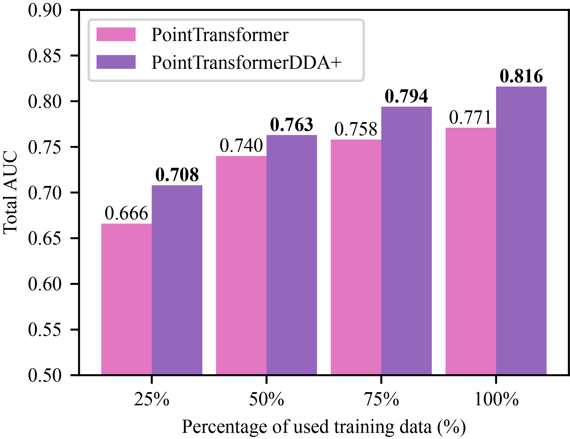
Figure 5: Performance compassion with different percentages of training WSIs.

IHC2+ Subset Analysis

In real clinical scenarios IHC score 2+, pathologists cannot assess the HER2 status from IHC and require further expensive ISH tests. However, Table 6 shows that our model still achieves impressive performance with an average AUC $>$ 0.7 in the test set. It can bring us an opportunity to reduce the reliance on ISH tests, thereby offering cost savings and faster HER2 status assessment.

Conclusion

Unlike MIL-based or graph-based methods, we regard a WSI as a point cloud with position information to derive the HER2 status from HE-stained WSIs, highlighting the effectiveness of point neural networks for WSI analysis. Specifically, a farthest cosine sampling is proposed to capture the long-range dependencies and aggregate most discriminative point features. Additionally, when utilizing federated learning, we proposed a dynamic distribution adjustment to mitigate the non-i.i.d. scenario of label imbalance in real-world WSIs. Extensive experiments have demonstrated the efficacy of our two components. Our models further achieve impressive performance in both unseen sites and IHC score 2+ subsets.

Roadmap of Appendix:

The Appendix includes details of WSI prepossess, WSI dataset and further experimental analysis of point transformer, and federated learning in our model.

Appendix A WSI Prepossess and Feature Extraction

We follow CLAM (Lu et al. 2021) to remove the white background region and then cut the tissue regions into patches with a fixed size of 256$\times$256 at 20$\times$ magnification ( 0.5$\mu m$/pixel) without overlap. For some WSIs that may not contain 20$\times$ magnification. For example, a WSI may only have 40$\times$, 10$\times$ magnification, we crop a larger size (40$\times$: 512$\times$512) or smaller size (10$\times$: 128$\times$128) and then resized to 256$\times$256 to guarantee the same field of view (FOV). The number of patches per WSI ranges from thousands to tens of thousands. The feature extraction in our study involved training of a nuclei segmentation model using the public nuclei dataset PanNuke (Gamper et al. 2019, 2020). The nuclei segmentation model is trained under an updated version of HTC-Lite from  (Wang et al. 2021) and is implemented using an open-source MMdetection toolbox.

Appendix B Details of WSI Dataset

The WSIs used in our study are involved with four publicly available datasets (Sites A, D, E, and F) and two internal datasets (Sites B and C) with the ethics committee’s approval. Site A is a well-known project TCGA-BRCA (Network 2012), and is widely used for WSI analysis. Site B’s WSIs are retrospectively collected from West China Hospital of Sichuan University. Site C’s WSIs are from out-of-hospital consultation cases of Sichuan University West China Hospital. Site D is the HEROHE Challenge (Conde-Sousa et al. 2022) dataset, which mainly contains biopsy WSIs, and Sites E and F are the Yale HER2 (Farahmand et al. 2022) dataset and the HER2C (Qaiser et al. 2017) datasets, respectively. All of the public datasets can be obtained from the public website offered in each paper. Note that Site F or HER2C dataset only includes an IHC score for each WSI without corresponding ISH score for IHC 2+. Thus we filter out IHC 2+ in Site F and regard the IHC 0/1+ as HER2- and IHC 3+ as HER2+.

During the training process, various data augmentation techniques are employed to augment the point data. These include random point dropout, point jitter, scaling in [0.8, 1.25], and shifting with a range of 0.1.

Appendix C Further Analysis of PointTransformer

The PointTransformer involves the random selection of 1024 points and the farthest cosine sampling, which can introduce a degree of randomness into the model’s results. Here we randomly repeat our model with 100 or even 1000 times to assess the stability of our model’s prediction. As shown in Table 7, we observe a 0.37% standard deviation in the test AUC, and the difference between the maximum and minimum AUC is only 0.022. These results demonstrate the robustness of our model to random sampling and indicate its consistent and reliable performance.

Repeat	Mean	Min	Max	Max-Min
100	0.805±0.0037	0.796	0.817	0.021
1000	0.806±0.0036	0.795	0.817	0.022

Table 7: Effects of randomness in PointTransformerDDA+.

Position	Average	Site A	Site B	Site C	Site D
0	0.700	0.670	0.721	0.704	0.676
1	0.709	0.663	0.733	0.698	0.714
Pos	0.765	0.707	0.805	0.787	0.696
Pos + Aug	0.771	0.717	0.834	0.776	0.721

Table 8: The effects of position information and point data augmentation in PointTransformer.

Table 8 shows that point data augmentation can increase HER2 prediction performance (AUC: 0.771 vs 0.765). Note that point augmentation is another feature that does not exist in the existing methods. We also evaluate the position effect by replacing the point position information with 0 or 1. In Table 8, we can observe that the model’s performance significantly decreases when position information is omitted. This highlights the importance of incorporating point position information for WSI analysis.

Appendix D Further Analysis of Federated Learning

In this section, we first evaluate the effect of group normalization’s number selection. Table 9 shows that our data is very sensitive to the choice of group number. Extreme group numbers (1: Layer Normalization, Max: Instance Normalization) and small group numbers lead to poor performance. On the other hand, group numbers 8 or 32 exhibit improved performance. Therefore, while group normalization can yield favorable results, it requires careful selection of the group number for our real-world WSIs.

Group Number	Average	Site A	Site B	Site C	Site D
1 (Layer Norm)	0.688	0.638	0.700	0.694	0.678
2	0.595	0.528	0.635	0.579	0.607
4	0.659	0.586	0.655	0.626	0.653
8	0.783	0.733	0.832	0.775	0.768
16	0.757	0.720	0.805	0.738	0.770
32	0.782	0.755	0.833	0.778	0.767
64	0.771	0.739	0.828	0.775	0.754
MAX (Instance Norm)	0.532	0.523	0.538	0.529	0.542

Table 9: Performance of the point transformer using group normalization with different group numbers.

Considering the variations in hardware and network quality, different sites may experience delays in communication frequency. We simulate a scene in which sites communicate with different paces ranging from 1 to 32. Figure 6 represents that our proposed PointTransformerDDA+ is more robust compared to the base PointTransformer, which demonstrates the effectiveness of our proposed components. Even with a pace of 32, our model still yields an AUC of 0.738, while the base PointTransformer shows a large performance decrement.

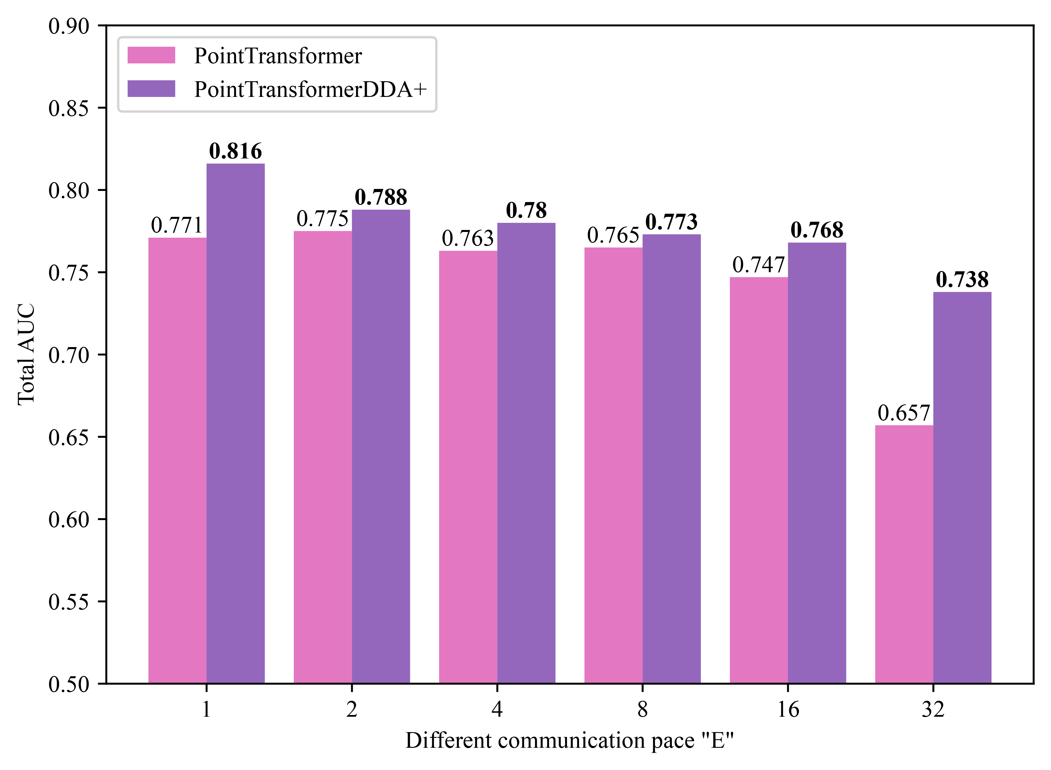
Figure 6: Performance compassion with different communication paces E.

Appendix E Model Visualization

We further try to visualize our model using integrated gradients (Sundararajan, Taly, and Yan 2017). Generally pathologists should access the HER2 status from IHC-stained WSI as shown in the right part of Figure 7. Deriving HER2 status from HE-stained WSI is challenging compared to IHC-stained WSI. However, our model can capture the deep IHC-stained area from HE-stained WSI as shown in the left part of Figure 7.

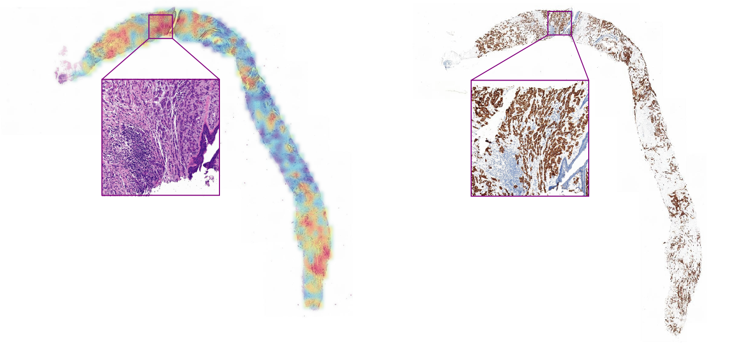
Figure 7: Visualization of a representative HE-stained WSI and its corresponding IHC-stained WSI with IHC score 3+.

References

- Chen et al. (2021a) Chen, R. J.; Lu, M. Y.; Shaban, M.; Chen, C.; Chen, T. Y.; Williamson, D. F. K.; and Mahmood, F. 2021a. Whole slide images are 2D point clouds: Context-aware survival prediction using patch-based graph convolutional networks. In Medical Image Computing and Computer Assisted Intervention, 339–349. Springer.
- Chen et al. (2020) Chen, R. J.; Lu, M. Y.; Wang, J.; Williamson, D. F.; Rodig, S. J.; Lindeman, N. I.; and Mahmood, F. 2020. Pathomic fusion: an integrated framework for fusing histopathology and genomic features for cancer diagnosis and prognosis. IEEE Transactions on Medical Imaging, 41: 757–770.
- Chen et al. (2021b) Chen, R. J.; Lu, M. Y.; Weng, W.-H.; Chen, T. Y.; Williamson, D. F.; Manz, T.; Shady, M.; and Mahmood, F. 2021b. Multimodal co-attention transformer for survival prediction in gigapixel whole slide images. In Proceedings of the IEEE/CVF International Conference on Computer Vision, 4015–4025.
- Conde-Sousa et al. (2022) Conde-Sousa, E.; Vale, J.; Feng, M.; Xu, K.; Wang, Y.; Mea, V. D.; Barbera, D. L.; Montahaei, E.; Baghshah, M. S.; Turzynski, A.; Gildenblat, J.; Klaiman, E.; Hong, Y.; Aresta, G.; Araújo, T.; Aguiar, P.; Eloy, C.; and Polónia, A. 2022. HEROHE challenge: Predicting HER2 status in breast cancer from hematoxylin-eosin whole-slide imaging. Journal of Imaging, 8(8): 213.
- Du et al. (2022) Du, Z.; Sun, J.; Li, A.; Chen, P.-Y.; Zhang, J.; Li, H. H.; and Chen, Y. 2022. Rethinking normalization methods in federated learning. In Proceedings of the 3rd International Workshop on Distributed Machine Learning, 16–22.
- Farahmand et al. (2022) Farahmand, S.; Fernandez, A. I.; Ahmed, F. S.; Rimm, D. L.; Chuang, J. H.; Reisenbichler, E.; and Zarringhalam, K. 2022. Deep learning trained on hematoxylin and eosin tumor region of Interest predicts HER2 status and trastuzumab treatment response in HER2+ breast cancer. Modern Pathology, 35(1): 44–51.
- Gamper et al. (2019) Gamper, J.; Koohbanani, N. A.; Benes, K.; Khuram, A.; and Rajpoot, N. 2019. PanNuke: an open pan-cancer histology dataset for nuclei instance segmentation and classification. In European Congress on Digital Pathology, 11–19.
- Gamper et al. (2020) Gamper, J.; Koohbanani, N. A.; Graham, S.; Jahanifar, M.; Khurram, S. A.; Azam, A.; Hewitt, K.; and Rajpoot, N. 2020. PanNuke dataset extension, insights and baselines. arXiv:2003.10778.
- Guan and Liu (2023) Guan, H.; and Liu, M. 2023. Federated learning for medical image analysis: A survey. arXiv:2306.05980.
- Guo et al. (2021) Guo, M.; Cai, J.; Liu, Z.; Mu, T.; Martin, R. R.; and Hu, S. 2021. PCT: Point cloud transformer. Computational Visual Media, 7: 187–199.
- Hamilton, Ying, and Leskovec (2017) Hamilton, W.; Ying, Z.; and Leskovec, J. 2017. Inductive representation learning on large graphs. In Advances in Neural Information Processing Systems, 1025–1035.
- Hou et al. (2022) Hou, W.; Yu, L.; Lin, C.; Huang, H.; Yu, R.; Qin, J.; and Wang, L. 2022. H^2-MIL: Exploring hierarchical representation with heterogeneous multiple instance learning for whole slide image analysis. In Proceedings of the AAAI Conference on Artificial Intelligence, 933–941.
- Hsieh et al. (2020) Hsieh, K.; Phanishayee, A.; Mutlu, O.; and Gibbons, P. 2020. The non-iid data quagmire of decentralized machine learning. In International Conference on Machine Learning, 4387–4398. PMLR.
- Hu et al. (2022) Hu, Z.; Shaloudegi, K.; Zhang, G.; and Yu, Y. 2022. Federated learning meets multi-objective optimization. IEEE Transactions on Network Science and Engineering, 9(4): 2039–2051.
- Ilse, Tomczak, and Welling (2018) Ilse, M.; Tomczak, J.; and Welling, M. 2018. Attention-based deep multiple instance learning. In International Conference on Machine Learning, 2127–2136. PMLR.
- Jiang, Wang, and Dou (2022) Jiang, M.; Wang, Z.; and Dou, Q. 2022. HarmoFL: Harmonizing local and global drifts in federated learning on heterogeneous medical images. In Proceedings of the AAAI Conference on Artificial Intelligence, 1087–1095.
- Kang et al. (2020) Kang, B.; Xie, S.; Rohrbach, M.; Yan, Z.; Gordo, A.; Feng, J.; and Kalantidis, Y. 2020. Decoupling representation and classifier for long-tailed recognition. In International Conference on Learning Representations, 1–16.
- Kather et al. (2020) Kather, J. N.; Heij, L. R.; Grabsch, H. I.; Loeffler, C.; Echle, A.; Muti, H. S.; Krause, J.; Niehues, J. M.; Sommer, K. A.; Bankhead, P.; et al. 2020. Pan-cancer image-based detection of clinically actionable genetic alterations. Nature Cancer, 1(8): 789–799.
- Lee, Shin, and Kim (2021) Lee, H.; Shin, S.; and Kim, H. 2021. ABC: Auxiliary balanced classifier for class-imbalanced semi-supervised learning. In Neural Information Processing Systems, 7082–7094.
- Lee et al. (2022) Lee, Y.; Park, J. H.; Oh, S.; Shin, K.; Sun, J.; Jung, M.; Lee, C.; Kim, H.; Chung, J.-H.; Moon, K. C.; et al. 2022. Derivation of prognostic contextual histopathological features from whole-slide images of tumours via graph deep learning. Nature Biomedical Engineering, 1–15.
- Li et al. (2022) Li, B.; Li, F.; Liu, Z.; Xu, F.; Ye, G.; Li, W.; Zhang, Y.; Zhu, T.; Shao, L.; Chen, C.; et al. 2022. Deep learning with biopsy whole slide images for pretreatment prediction of pathological complete response to neoadjuvant chemotherapy in breast cancer: A multicenter study. The Breast, 66: 183–190.
- Li, Li, and Eliceiri (2020) Li, B.; Li, Y.; and Eliceiri, K. W. 2020. Dual-stream multiple instance learning network for whole slide image classification with self-supervised contrastive learning. In Proceedings of the IEEE/CVF Conference on Computer Vision and Pattern Recognition, 14313–14323.
- Li et al. (2020) Li, T.; Sahu, A. K.; Zaheer, M.; Sanjabi, M.; Talwalkar, A.; and Smith, V. 2020. Federated optimization in heterogeneous networks. In Proceedings of Machine Learning and Systems, 429–450.
- Lin et al. (2017) Lin, T. Y.; Dollar, P.; Girshick, R.; He, K.; Hariharan, B.; and Belongie, S. 2017. Feature pyramid networks for object detection. In Proceedings of the IEEE/CVF Conference on Computer Vision and Pattern Recognition, 936–944.
- Liu et al. (2021) Liu, Z.; Lin, Y.; Cao, Y.; Hu, H.; Wei, Y.; Zhang, Z.; Lin, S.; and Guo, B. 2021. Swin transformer: Hierarchical vision transformer using shifted windows. In Proceedings of the IEEE/CVF International Conference on Computer Vision, 9992–10002.
- Lu et al. (2022a) Lu, D.; Xie, Q.; Wei, M.; Gao, K.; Xu, L.; and Li, J. 2022a. Transformers in 3D point clouds: A survey. arXiv:2205.07417.
- Lu et al. (2022b) Lu, M. Y.; Chen, R. J.; Kong, D.; Lipkova, J.; Singh, R.; Williamson, D. F.; Chen, T. Y.; and Mahmood, F. 2022b. Federated learning for computational pathology on gigapixel whole slide images. Medical Image Analysis, 76: 102298.
- Lu et al. (2021) Lu, M. Y.; Williamson, D. F.; Chen, T. Y.; Chen, R. J.; Barbieri, M.; and Mahmood, F. 2021. Data-efficient and weakly supervised computational pathology on whole-slide images. Nature Biomedical Engineering, 5(6): 555–570.
- Lu et al. (2022c) Lu, W.; Toss, M.; Dawood, M.; Rakha, E.; Rajpoot, N.; and Minhas, F. 2022c. SlideGraph+: Whole slide image level graphs to predict HER2 status in breast cancer. Medical Image Analysis, 80: 102486.
- McMahan et al. (2017) McMahan, B.; Moore, E.; Ramage, D.; Hampson, S.; and y Arcas, B. A. 2017. Communication-efficient learning of deep networks from decentralized data. In Artificial Intelligence and Statistics, 1273–1282. PMLR.
- Network (2012) Network, T. C. G. A. 2012. Comprehensive molecular portraits of human breast tumors. Nature, 490: 61–70.
- Ogier du Terrail et al. (2023) Ogier du Terrail, J.; Leopold, A.; Joly, C.; Béguier, C.; Andreux, M.; Maussion, C.; Schmauch, B.; Tramel, E. W.; Bendjebbar, E.; Zaslavskiy, M.; et al. 2023. Federated learning for predicting histological response to neoadjuvant chemotherapy in triple-negative breast cancer. Nature Medicine, 29: 135–146.
- Oh and Bang (2019) Oh, D. Y.; and Bang, Y. 2019. HER2-targeted therapies — a role beyond breast cancer. Nature Reviews Clinical Oncology, 17: 33–48.
- Qaiser et al. (2017) Qaiser, T.; Mukherjee, A.; Reddy Pb, C.; Munugoti, S. D.; Tallam, V.; Pitkäaho, T.; Lehtimäki, T.; Naughton, T.; Berseth, M.; Pedraza, A.; et al. 2017. HER2 challenge contest: a detailed assessment of automated HER2 scoring algorithms in whole slide images of breast cancer tissues. Histopathology, 72: 227–238.
- Qi et al. (2017a) Qi, C. R.; Su, H.; Mo, K.; and Guibas, L. J. 2017a. PointNet: Deep learning on point sets for 3D classification and segmentation. In Proceedings of the IEEE/CVF Conference on Computer Vision and Pattern Recognition, 652–660.
- Qi et al. (2017b) Qi, C. R.; Yi, L.; Su, H.; and Guibas, L. J. 2017b. PointNet++: Deep hierarchical feature learning on point sets in a metric space. In Advances in Neural Information Processing Systems, 5105–5114.
- Shao et al. (2021) Shao, Z.; Bian, H.; Chen, Y.; Wang, Y.; Zhang, J.; Ji, X.; and Zhang, Y. 2021. TransMIL: Transformer based correlated multiple instance learning for whole slide image classification. In Advances in Neural Information Processing Systems, 2136–2147.
- Shao et al. (2023) Shao, Z.; Chen, Y.; Bian, H.; Zhang, J.; Liu, G.; and Zhang, Y. 2023. HVTSurv: Hierarchical vision transformer for patient-level survival prediction from whole slide image. In Proceedings of the AAAI Conference on Artificial Intelligence, 2209–2217.
- Shen et al. (2022) Shen, Y.; Liu, L.; Tang, Z.; Chen, Z.; Ma, G.; Dong, J.; Zhang, X.; Yang, L.; and Zheng, Q. 2022. Explainable survival analysis with convolution-involved vision transformer. In Proceedings of the AAAI Conference on Artificial Intelligence, 2207–2215.
- Sundararajan, Taly, and Yan (2017) Sundararajan, M.; Taly, A.; and Yan, Q. 2017. Axiomatic attribution for deep networks. In International Conference on Machine Learning, 3319–3328. PMLR.
- Wang et al. (2021) Wang, J.; Zhang, W.; Zang, Y.; Cao, Y.; Pang, J.; Gong, T.; Chen, K.; Liu, Z.; Loy, C. C.; and Lin, D. 2021. Seesaw loss for long-tailed instance segmentation. In Proceedings of the IEEE/CVF Conference on Computer Vision and Pattern Recognition, 9695–9704.
- Wang et al. (2019) Wang, Y.; Sun, Y.; Liu, Z.; Sarma, S. E.; Bronstein, M. M.; and Solomon, J. M. 2019. Dynamic graph cnn for learning on point clouds. ACM Transactions on Graphics (tog), 38(5): 1–12.
- Wolff et al. (2018) Wolff, A. C.; Hammond, M. E. H.; Allison, K. H.; Harvey, B. E.; Mangu, P. B.; Bartlett, J. M.; Bilous, M.; Ellis, I. O.; Fitzgibbons, P.; Hanna, W.; et al. 2018. Human epidermal growth factor receptor 2 testing in breast cancer: American Society of Clinical Oncology/College of American Pathologists clinical practice guideline focused update. Archives of Pathology & Laboratory Medicine, 142(11): 1364–1382.
- Xu et al. (2019) Xu, K.; Hu, W.; Leskovec, J.; and Jegelka, S. 2019. How powerful are graph neural networks? In International Conference on Learning Representations, 1–17.
- Xu et al. (2018) Xu, K.; Li, C.; Tian, Y.; Sonobe, T.; Kawarabayashi, K.-i.; and Jegelka, S. 2018. Representation learning on graphs with jumping knowledge networks. In International Conference on Machine Learning, 5453–5462. PMLR.
- Zhao et al. (2021) Zhao, H.; Jiang, L.; Jia, J.; Torr, P. H.; and Koltun, V. 2021. Point Transformer. In Proceedings of the IEEE/CVF International Conference on Computer Vision, 16259–16268.
- Zhuang and Lyu (2023) Zhuang, W.; and Lyu, L. 2023. Is normalization indispensable for multi-domain federated learning? arXiv:2306.05879.