Comparison of time-of-flight with MIEZE spectroscopy of H₂O: Necessity to go beyond the spin-echo approximation

Abstract

Here, we discuss the comparability of data acquisitioned with the Modulation of IntEnsity with Zero Effort data, a neutron spin-echo (NSE) technique to neutron Time-of-Flight (ToF) spectroscopy data. As a NSE technique MIEZE records the intermediate scattering function $\mathcal{I}(Q,\tau)$ making it necessary to perform a Fourier transform to directly compare it to $S(Q,E)$, measured by ToF spectroscopy. Transforming either data set into the complementary parameter space requires detailed knowledge of detector efficiency, instrumental resolution, and background. We discuss these aspects by comparing measurements on pure water performed on the spectrometers RESEDA and TOFTOF under the same experimental conditions. Additionally, we discuss the data evaluation of spin-echo data beyond the SE approximation, which limits these techniques to small energy transfers.

1 Introduction

Quasielastic neutron scattering (QENS) describes a limiting case of inelastic neutron scattering, where energy transfers are small with respect to the energy of the incoming neutron. Currently three spectrometer types are ideally suited to study QENS: backscattering (BS) spectrometers, time-of-flight (ToF) spectrometers, and neutron spin-echo (NSE) spectrometers.

While BS and ToF spectrometry measure the change of the neutrons energy via a crystal analyzer or the neutron time-of-flight respectively, NSE uses the precession of the neutron spin in a magnetic field to encode this information. Following from this, BS and ToF uncover the dynamic structure factor $S(Q,E)$, while NSE elucidates the intermediate scattering function $\mathcal{I}(Q,\tau$). Both approaches offer their advantages and disadvantages, however this conceptual difference in the collected data has divided the QENS community. One goal of this manuscript is to highlight the complementarity of NSE and ToF, and to show how data can be compared, when considering all instrumental resolution effects.

Neutron ToF spectroscopy uses the measured time-of-flight of a neutron between two known points in space to determine the neutron’s kinetic energy. In indirect geometry instruments, the sample is illuminated by a pulsed white beam, and the energy of the scattered beam is determined using a crystal analyzer. For direct geometry instruments, the incident beam is monochromatized either by a crystal monochromator or by a set of at least two choppers. In both cases the final energy is determined using the fixed distance from sample to detector.

ToF spectrometers have the advantage of large detector coverage, however at continuous (reactor) sources, they suffer from a dramatic reduction in flux by chopping the beam. On pulsed (spallation) sources, ToF instruments are the natural choice of spectrometer. These instruments are versatile, since their resolution reaches down to a few $\mu$eV (e.g. LET [BEWLEY2011, Nilsen_2017], or IN5 [Ollivier2002], [Ollivier2011]) or use incident energies of up to 1000 meV (e.g. MARI) [ANDERSEN1996, le2022upgrade]). Options for polarized beams, as well as polarization analysis exist.

ToF and BS cover simultaneously a large momentum transfer range, $Q$, that encompasses atomic and inter atomic distances (below $10\text{\,}\mathrm{\SIUnitSymbolAngstrom}$) but lack resolution when it comes to mesoscopic length scales (above $10\text{\,}\mathrm{\SIUnitSymbolAngstrom}$), due to their relaxed beam collimation. These techniques are therefore ideally suited to measure molecular reorientation, hydrogen diffusion or liquid dynamics and many more. However, they cannot resolve the dynamics of mesoscopic objects such as domain motions in macro-molecules, polymer chain-dynamics or emergent excitations in quantum magnets due to the combination of intermediate energy resolution and the coarse momentum transfer resolution at small $Q$.

Alternatively, neutron spin-echo techniques achieve very high energy resolution (down to $<$1\text{\,}\mathrm{neV}$$ [JNSE, IN15]) in combination with very high neutron intensity through the decoupling of the energy resolution of the instrument from the wavelength spread of the neutrons [1972Mezei, 1980Mezei]. In NSE, the Larmor precession phase of the neutron spin, acquired in a well-defined magnetic field region before and after the sample, are compared. A scattering process within the sample leads to a phase difference resulting in a reduction in neutron polarization at the detector. NSE is especially well suited for the investigation of slow ( $\sim$1\text{\,}\mathrm{ns}$$ to $\sim$100\text{\,}\mathrm{ns}$$) relaxation processes. Typical problems are: thermal fluctuations of surfactant membranes in microemulsions, the molecular rheology of polymer melts, thermally activated domain motion in proteins, relaxation phenomena in networks and rubbers, interface fluctuations in complex fluids and polyelectrolytes; transport processes in polymeric electrolytes and gel systems, the domain dynamics of proteins and enzymes transport process through cell membranes. [Mihailescu2001, Schleger1998, Bu2005]

While classical NSE has established itself as an excellent probe for soft-matter systems, it has a few shortcomings when approaching problems in hard condensed matter and magnetism: depolarizing samples or sample environments lead to a loss in signal. Therefore, measurements under such conditions are cumbersome, and come with a decrease in neutron intensity at the sample position (e.g. ferromagnetic NSE) [Mezei2009, Keller2021]. The MIEZE (modulation of intensity with zero effort) variant of NSE circumvents this issue, by limiting the manipulation of the neutron spin to the primary spectrometer arm.

Analogously to neutron resonance spin-echo (NRSE) [1987Golub, 1992Gaehler], MIEZE uses RF spin-flippers instead of large solenoids to create the precession zone for the neutron spin. Since these RF flippers are very compact, they allow for the insertion of a field subtraction coil between them [2019Jochum, 2005Haeussler], extending the dynamic range of MIEZE (and NRSE) several orders of magnitude towards shorter echo times (e.g. RESEDA at $4.5\text{\,}\mathrm{\SIUnitSymbolAngstrom}$ $\rightarrow\tau_{\mathrm{min}}$ = $0.1\text{\,}\mathrm{fs}$). The advancement towards shorter echo times, and therefore larger energy transfers, has challenged the spin-echo (SE) approximation, which has been the standard framework to understand NSE but only holds true for small energy transfers [2019Franz2, 2019Franz3]. Here, we want to show the utility of spin-echo techniques beyond the SE approximation, using established numerical methods. However, conceptional challenges implied by the SE approximation, such as the per se unknown energy and wavevector transfer, remain and limits MIEZE investigations to dispersionless excitations if no additional sample information, such as molecular dynamics (MD) simulations or input from other neutron spectroscopy experiments, are available. [Keller2021]

2 Theoretical framework

NSE techniques use the precession of the neutron spin in magnetic fields to detect energy transfer during scattering events. For a detailed description we refer to the book by Mezei [mezei2002neutron]. Here, we will limit ourselves to the concepts needed to discuss the SE approximation and its implications. For this, we start by defining the precession angle of a neutron travelling with a velocity $v$ through a magnetic field of field strength $B$, and length $L$:

$$\Phi=\Phi_{0}+\frac{\gamma BL}{v},$$ (1)

where $\gamma$ is the neutron’s gyromagnetic ratio ($\gamma=$183.25\text{\,}\mathrm{MHz}\text{\,}{\mathrm{T}}^{-1}$$ for angles in radiant). Without loss of generality, we assume $\Phi_{0}=0$ in the following. In an NSE setup, a neutron travels through a well defined magnetic field region ($B_{1}$, $L_{1}$) before the sample position, and then through another well defined field region after the sample position ($B_{2}$, $L_{2}$). The phase $\Phi_{D}$ of the neutron at the detector position can then be written as:

$$\Phi_{D}=\Phi_{1}+\Phi_{2}=\frac{\gamma B_{1}L_{1}}{v_{1}}+\frac{\gamma B_{2}L_{2}}{v_{2}}.$$ (2)

Length and field strength are chosen such that: $L_{2}$ = $L_{1}$ = $L$, and $B_{2}$ = $-B_{1}$ = $B$. Therefore, equation 2 becomes

$$\Phi_{D}=\gamma BL\cdot\left(\frac{1}{v_{1}}-\frac{1}{v_{2}}\right).$$ (3)

We can write $v_{2}=v_{1}+\Delta v$, where $\Delta v$ is the change in velocity the neutron experiences when interacting with a sample positioned between the precision fields, thus:

$$\Phi_{D}=\gamma BL\cdot\left(\frac{1}{v_{1}}-\frac{1}{v_{1}+\Delta v}\right).$$ (4)

For a purely elastic scatterer $\Delta v$ = 0, and therefore $\Phi_{D}$ = 0. If the neutron exchanges energy with the sample $\Delta v$ $\neq$ 0, this is detected as a phase shift $\Phi_{D}$. The change in neutron energy during such an interaction, can be written as:

$$E =\frac{m}{2}\cdot(v_{2}^{2}-v_{1}^{2})$$ (5)

$$=\frac{m}{2}\cdot((v_{1}+\Delta v)^{2}-v_{1}^{2})$$

$$=\frac{m}{2}\cdot(2v_{1}\Delta v+\Delta v^{2})$$

The SE approximation assumes that the energy transfer ($E$) is much smaller than the kinetic energy of the incoming neutrons, i.e., $E\ll\frac{1}{2}mv_{1}^{2}$ and thus $\Delta v\ll v_{1}$, from which follows:

$$E\simeq mv_{1}\Delta v$$ (6)

Thus, $\Delta v$ can be written as:

$$\Delta v\simeq\frac{E}{mv_{1}}$$ (7)

Within the spin-echo approximation $\Delta v+v_{1}\simeq v_{1}$ and therefore:

$$\Phi_{D} \simeq\gamma BL\cdot\frac{\Delta v}{v_{1}^{2}}$$ (8)

$$\simeq\gamma BL\cdot\frac{E}{mv_{1}^{3}}\overset{!}{=}\tau\frac{E}{\hbar}$$

Equation 8 defines the spin-echo time $\tau$ as a proportionality factor between the neutron phase $\Phi_{D}$ at the detector and the energy transfer $E$.

Using a neutron polarization analyzer and a neutron detector at a certain scattering angle 2$\vartheta$ the number of polarized neutrons are recorded. This corresponds to the expectation value of $\cos(\Phi_{D}$) over scattered neutrons ($\langle\cos\Phi_{D}\rangle$) in 2$\vartheta$. Within the spin echo approximation ($\lambda_{i}\,\approx\,\lambda_{f}$) $Q$ is well defined via $2\vartheta$ and the probability of a scattering event with energy transfer $E$ is given by $S(Q,E)$. This assumption leads to:

$$P_{x}=\langle\cos\Phi_{D}\rangle_{E} \simeq\frac{\int_{-\infty}^{\infty}S(Q,E)\cos\Phi_{D}\mathrm{d}E}{\int_{-\infty}^{\infty}S(Q,E)\mathrm{d}E}$$ (9)

$$\simeq\frac{\int_{-\infty}^{\infty}S(Q,E)\cos(\frac{E}{\hbar}\tau)\mathrm{d}E}{\int_{-\infty}^{\infty}S(Q,E)\mathrm{d}E}.$$

The nominator of Equation 9 is the cosine Fourier transform of $S(Q,E)$, which is known to be the real part of the time dependent correlation function, the so-called intermediate scattering function $\mathcal{I}(Q,\tau)$. The denominator is the static structure factor $S(Q)$. Therefore:

$$P_{x}=\frac{Re(\mathcal{F}(S(Q,E)))}{S(Q)}=\frac{\mathcal{I}(Q,\tau)}{\mathcal{I}(Q,0)}$$ (10)

Within the SE approximation, this leads to the interpretation that the measured polarization $P_{x}$ is essentially the energy cosine-transform of $S(Q,E)$ normalized to the static scattering factor, or, expressed in the time domain, the intermediate scattering function normalized to its value at zero Fourier time.

Since the SE approximation implies that $k\lambda_{f}\sim\lambda_{i}$ the momentum transfer $Q$ can simply be related to the scattering angle via:

$$Q=\frac{4\pi}{{\lambda}}\mathrm{sin}\left(\frac{2\vartheta}{2}\right).$$ (11)

As a consequence it is sufficient to only consider the dynamic structure factor $S(Q,E)$ instead of the double differential cross section $\frac{\mathrm{d}^{2}\sigma}{\mathrm{d}\Omega\mathrm{d}E}$ when determining the probability for the scattering event, as the pre-factor (see eq. 12) approaches $k_{f}/k_{i}\approx 1$. [zolnierczuk2019efficient].

2.1 NSE beyond the SE approximation

Assuming a typical wavelength of $6$ Å for the incoming neutrons, and thus a kinetic energy of $2.27$ meV, the SE approximation holds true for quasi-elastic scattering processes with energies in the $\mu$eV-range (see fig. 1). Accordingly, NSE is not suited to investigate processes with energy transfers in the meV-range, including inelastic processes. $\mathcal{I}(Q,\tau)$ as it is measured is not normalized to the full $\int_{-\infty}^{\infty}{S(Q,E)dE}$ but to a structure factor where the integral is taken only over the band-pass of the spectrometer [Richter1998]. The lower boundary of this integral is given by $-E_{in}$, the incoming neutron energy, while the upper boundary is given by the maximum wavelength accepted by the neutron analyzer.

To go beyond the SE approximation the explicit expression for the phase at the detector $\Phi_{D}$ needs to be used (see eq. 4) and the conservation of energy and momentum need to be considered. Furthermore, the scattering angle $2\vartheta$ needs to be used instead of $Q$ and the dynamic structure factor $S(Q,E)$ needs to be replaced by the double differential scattering cross section $\frac{\mathrm{d}^{2}\sigma}{\mathrm{d}\Omega\mathrm{d}E}$.

Therefore, eq. 9 becomes

$$P_{x}=\langle\cos\Phi_{D}\rangle_{E} =\frac{\int_{-\infty}^{\infty}\frac{\mathrm{d}^{2}\sigma}{\mathrm{d}\Omega\mathrm{d}E}\cos\Phi_{D}\mathrm{d}E}{\int_{-\infty}^{\infty}\frac{\mathrm{d}^{2}\sigma}{\mathrm{d}\Omega\mathrm{d}E}\mathrm{d}E}$$ (12)

$$=\frac{\int_{-\infty}^{\infty}\frac{k_{f}}{k_{i}}S(2\vartheta,E)\cdot\mathrm{cos}\left(\gamma BL\left(\frac{1}{v_{1}+\Delta v}-\frac{1}{v_{1}}\right)\right)\mathrm{d}E}{\int_{-\infty}^{\infty}\frac{k_{f}}{k_{i}}S(2\vartheta,E)\mathrm{d}E}.$$ (13)

2.2 The MIEZE method

The data presented here was recorded using the Modulation of IntEnsity with Zero Effort (MIEZE) technique. Analoguously to neutron resonant spin-echo, in a MIEZE setup the large solenoids that create the spin precession zones are replaced by pairs of resonant spin flippers. For MIEZE the spin flipper pair after the sample is removed, and the spin flippers before the sample are operated at different frequencies $f_{A}$ and $f_{B}$, and placed a distance $L_{AB}$ apart.

Analogously to classical NSE the spin phase at the detector can be defined as:

$$\Phi_{D}=2\pi f_{M}t_{D}-2\pi f_{M}\frac{L_{BD}}{v}+2\pi f_{A}\frac{L_{AB}}{v},$$ (14)

where $t_{D}$ is the time the neutron arrives at the detector, $v$ is the initial neutron velocity, $f_{M}=2(f_{B}-f_{A})$ the MIEZE frequency and $L_{BD}$ the distance between the second spin flipper and the detector. The MIEZE detector is placed such that the velocity dependent terms cancel out, simplifying the equation [1992Gaehler, 2019Jochum].

Energy transfers $E$ during the scattering event will induce a delay $\Delta t_{D}$ in the neutron propagation time over the distance $L_{SD}$:

$$\Delta t_{D}=L_{SD}\left(\frac{1}{v_{1}}-\frac{1}{\sqrt{v_{1}^{2}+2E/m}}\right).$$ (15)

This leads to a deviation of the spin phase at the detector:

$$\Delta\Phi_{D}=2\pi f_{M}\Delta t_{D},$$ (16)

which reduces the contrast.

Within the SE approximation, we can rewrite this equation, in complete analogy to classical NSE:

$$\Phi_{D}\simeq\frac{2\pi f_{M}L_{SD}\hbar}{mv_{1}^{3}}\frac{E}{\hbar}\overset{!}{=}\tau_{M}\frac{E}{\hbar},$$ (17)

such that the Fourier time $\tau_{M}$ serves as a proportionality factor between the detector phase and the energy transfer.

Averaging this effect over all possible energy transfers, in perfect analogy to the polarization $P_{x}$ for classical NSE (see. eq. 12), results in the most general expression for the so-called contrast:

$$C =\langle\cos\Phi_{D}\rangle_{E}=\left<\mathrm{cos}(2\pi f_{M}\Delta t_{D})\right>_{E}$$ (18)

$$=\frac{\int_{-\infty}^{\infty}\frac{\mathrm{d}^{2}\sigma}{\mathrm{d}\Omega\mathrm{d}E}\mathrm{cos}(2\pi f_{M}\Delta t_{D})\mathrm{d}E}{\int_{-\infty}^{\infty}\frac{\mathrm{d}^{2}\sigma}{\mathrm{d}\Omega\mathrm{d}E}\mathrm{d}E}$$ (19)

$$=\frac{\int_{-\infty}^{\infty}\frac{k_{f}}{k_{i}}S(2\vartheta,E)\mathrm{cos}\left(2\pi f_{M}L_{SD}\left(\frac{1}{v_{1}}-\frac{1}{\sqrt{v_{1}^{2}+2E/m}}\right)\right)\mathrm{d}E}{\int_{-\infty}^{\infty}\frac{k_{f}}{k_{i}}S(2\vartheta,E)\mathrm{d}E}.$$ (20)

2.3 Computation of the MIEZE contrast

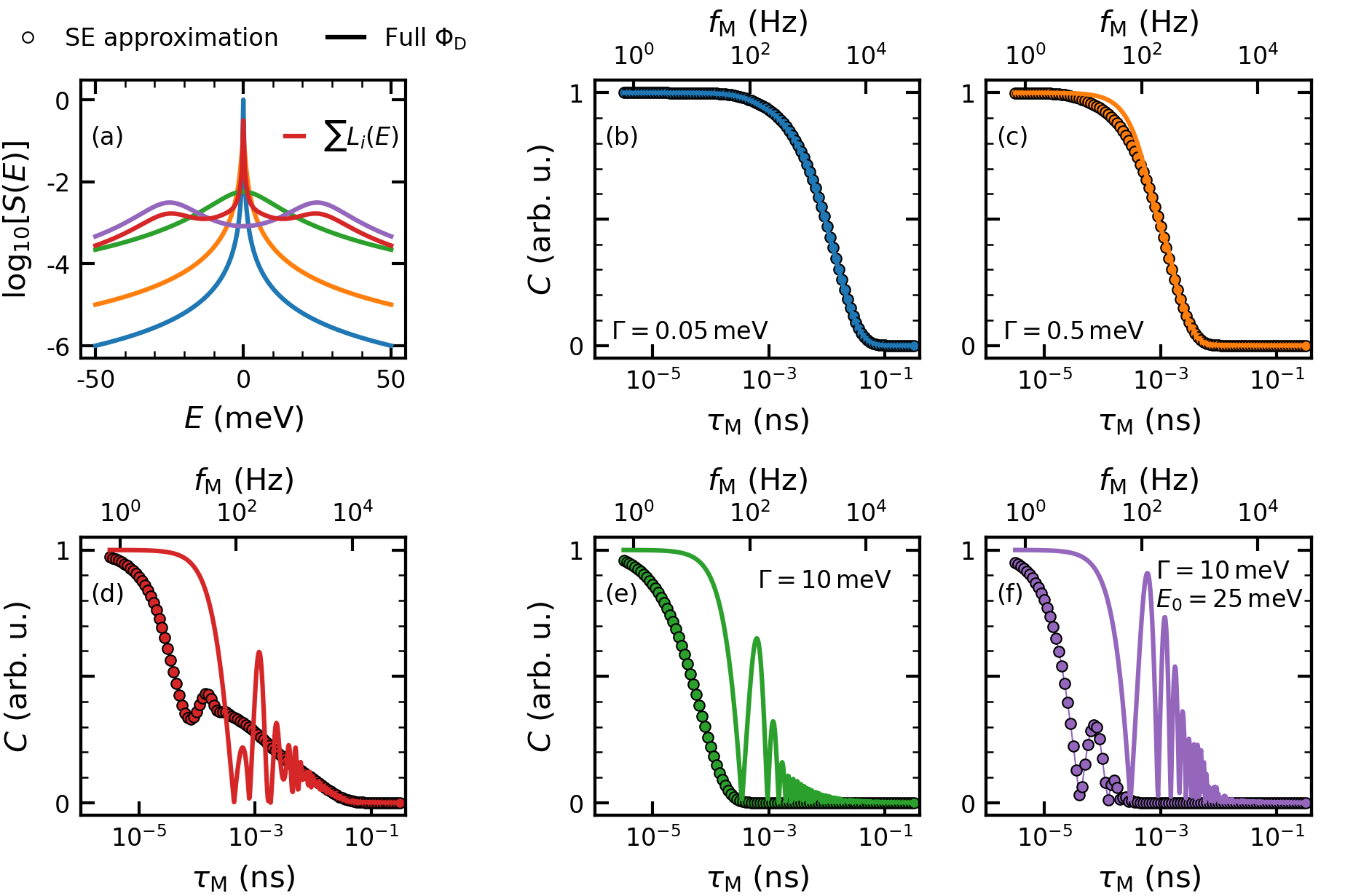
Figure 1: Visualization of the difference between spin-echo approximation and the full phase calculation. Subplot (a) shows five dynamic structure factors whose transformation into the time domain is shown in graphs (b)-(f) as indicated by their color. Three distributions model quasielastic scattering with $\Gamma=$0.05\text{\,}\mathrm{meV}$$ (blue), $\Gamma=$0.5\text{\,}\mathrm{meV}$$ (orange) and $\Gamma=$10.0\text{\,}\mathrm{meV}$$ (green). The purple line represents a broad, inelastic scattering process with $\Gamma=$10.0\text{\,}\mathrm{meV}$$ and $E_{0}=$25.0\text{\,}\mathrm{meV}$$. The red distribution is a sum of the previous described dynamic structure factors weighted by $\frac{1}{4}$. In (b)-(f) the transformation calculated in SE approximation is shown by circles, while the solid lines depict the result of equation 18. The wavelength of the incoming neutron beam was set to $6.0\text{\,}\mathrm{\SIUnitSymbolAngstrom}$ and assumed to be monochromatic.

To visualize the influence of the SE approximation, we computed the expected MIEZE contrasts for different dynamic structure factors $S(Q,E)$. We assumed a monochromatic neutron beam with a wavelength of $\lambda=6$Å, which corresponds to a kinetic energy of $2.27\text{\,}\mathrm{meV}$. Fig. 1(a) shows five Lorentzian distributions $S(2\vartheta,E)\propto\Gamma/(\Gamma^{2}+(E\pm E_{0})^{2})$, where $\Gamma$ is the linewidth of the distribution and $E_{0}$ the energy of the modeled excitation, corresponding to the center of the distribution. Quasielastic scattering is typically modeled by a Lorentzian with $E_{0}=0$, whereas inelastic contributions consist of two peaks centered around $\pm E_{0}$. Within the SE approximation the computation of the MIEZE-contrast is essentially a cosine Fourier transform of $S(E)$. Applying eq. 9 to the Lorentzian distributions shown in fig. 1(a) results in the curves represented by the circles in fig. 1(b)-(f). The curves comprise an exponential decay with $C\propto\mathrm{exp}(-\Gamma\tau_{M}/\hbar)$ modulated by a $\mathrm{cos}(\tau_{M}E_{0}/\hbar)$-term in case of an inelastic contribution.

In a MIEZE experiment, we measure the contrast given by eq. 18, which is shown by the continuous lines in fig. 1(b)-(f). It can be seen in fig. 1 that only for the narrowest Lorentzian both transformations result in a similar contrast curve. Already for widths of around $\Gamma=$0.2\text{\,}\mathrm{meV}$$, we observe deviations. These deviations become severe for distributions with $\Gamma>$0.5\text{\,}\mathrm{meV}$$, which corresponds to roughly $22\text{\,}\mathrm{\char 37\relax}$ of the kinetic energy of the incoming neutrons, as can be seen in fig. 1(e) and (c).

The calculations shown in figure 1 demonstrate that the non-linear phase in the cosine-term and the $k_{\mathrm{f}}/k_{\mathrm{i}}$ factor create an oscillation on $C$ for a broad quasielastic dynamic structure factor, which is absent in the SE approximation (see fig. 1 (c)). As a result, the oscillation that is characteristic for purely inelastic scattering is overlaid by this instrument dependent variation of the contrast. These two contributions can not be easily disentangled, although we have used extreme examples. Analysis of real world measurements requires an additional step of complexity by considering instrument parameters like detector efficiency [2019Koehli], wavelength band and beam divergence. Some details will be given below and a comprehensive account can be found in [beddrich2023consequences].

3 Experimental Methods

The intermediate scattering function of ultra pure (liquid Milli-Q™ultrapure) water was measured using the MIEZE option of the resonant spin-echo spectrometer RESEDA [reseda] at the Heinz Maier-Leibnitz Zentrum in Munich, Germany [2019Franz, 2019Franz2]. For the measurement, the water was kept in a Hellma macro cell with an optical path length of 1 mm. The cell was kept at a temperature of 300 K using a closed cycle cryostat in closed loop temperature control. The resolution curve was recorded, using carbon powder (a purely elastic scatterer) inside an identical Hellma macro cell. The complementary ToF measurement was performed with the instrument TOFTOF at the MLZ [TOFTOF, UNRUH2007]. Here, we measured the dynamic structure factor $S(2\vartheta,E)$ at $T=300$ K for a large angular range.

3.1 Data reduction

The neutron scattering data acquired have been reduced using standard procedures. In case of the MIEZE data, the reduction was done using the software package MIEZEPY as described in [MIEZEPY]. The process yields the contrast $C(2\vartheta,f_{\mathrm{M}})$ at a fixed scattering angle $2\vartheta$.

The ToF data was normalized to the incoming flux to account for natural flux fluctuations from the reactor source. To account for scattering off the cuvette an empty cell was measured and subsequently subtracted from the data. The detector itself was calibrated using a vanadium standard, taking into account a correction for the anisotropy of the Debye-Waller-factor of vanadium. The vanadium measurement was further used to determine the resolution of the elastic line. Subsequent to these corrections the energy transfer was calculated from the measured neutron time-of-flight. Finally, the data was binned in $E$, leading to a small energy offset of $-4.53(22)\text{\,}\mathrm{\SIUnitSymbolMicro eV}$. This is why, the elastic line determined from the water measurement was corrected by this offset. Knowing the energy transfer and the scattering angle $2\vartheta$ the momentum transfer $Q$ can be calculated. However, this step was omitted since a comparison to the RESEDA data is only possible for constant scattering angle $2\vartheta$. As a final step, the measured neutron intensity was corrected for the energy dependent detection efficiency [UNRUH2007] and for the $k_{\mathrm{f}}/k_{\mathrm{i}}$ factor in the double differential cross section.

4 Data analysis

We have pursued four approaches to compare the data measured at the different spectrometers. These approaches comprise

• direct transformation of the measured ToF spectrum into the time domain,

• simultaneous fit of a $S(2\vartheta,E)$ model function applied to both data sets, taking into account models for the instrument resolution, bandwidth and energy dependent detector efficiencies,

• inverse Fourier transformation of the measured MIEZE data into the energy domain based on Bayesian analysis, and

• numerical ray-tracing simulation of the RESEDA spectrometer.

However, only the first and second approach will be elucidated in detail.

4.1 Direct transformation approach

As motivated in sections 2.2 and 2.3, we need to go beyond the SE approximation to transform the ToF energy spectrum. The results of applying equations 9, and 18 to the data measured on TOFTOF in comparison to the data measured on RESEDA can be seen in figure 2, where different layers of complexity in the transformation have been added. Emphasizing the inadequacy of the SE approximation, the green markers have been calculated using the standard framework expressed by eq. 9, which are unable to describe the MIEZE data set. Adding the full expression of the MIEZE phase change $\Delta\Phi_{D}$ as well as the correction factor $k_{\mathrm{f}}/k_{\mathrm{i}}$ yields the orange curve that reproduces the characteristic oscillations in terms of their frequency but not with the correct amplitude. Factoring in the energy dependent detection efficiency of the CASCADE detector at RESEDA [2016Koehli], designated as $\varepsilon(E)$, achieves a reduction in the amplitude of the oscillations around $1.0\text{\times}{10}^{2}\text{\,}\mathrm{Hz}1.0\text{\times}{10}^{3}\text{\,}\mathrm{Hz}$ to the exact level seen in the original RESEDA data.

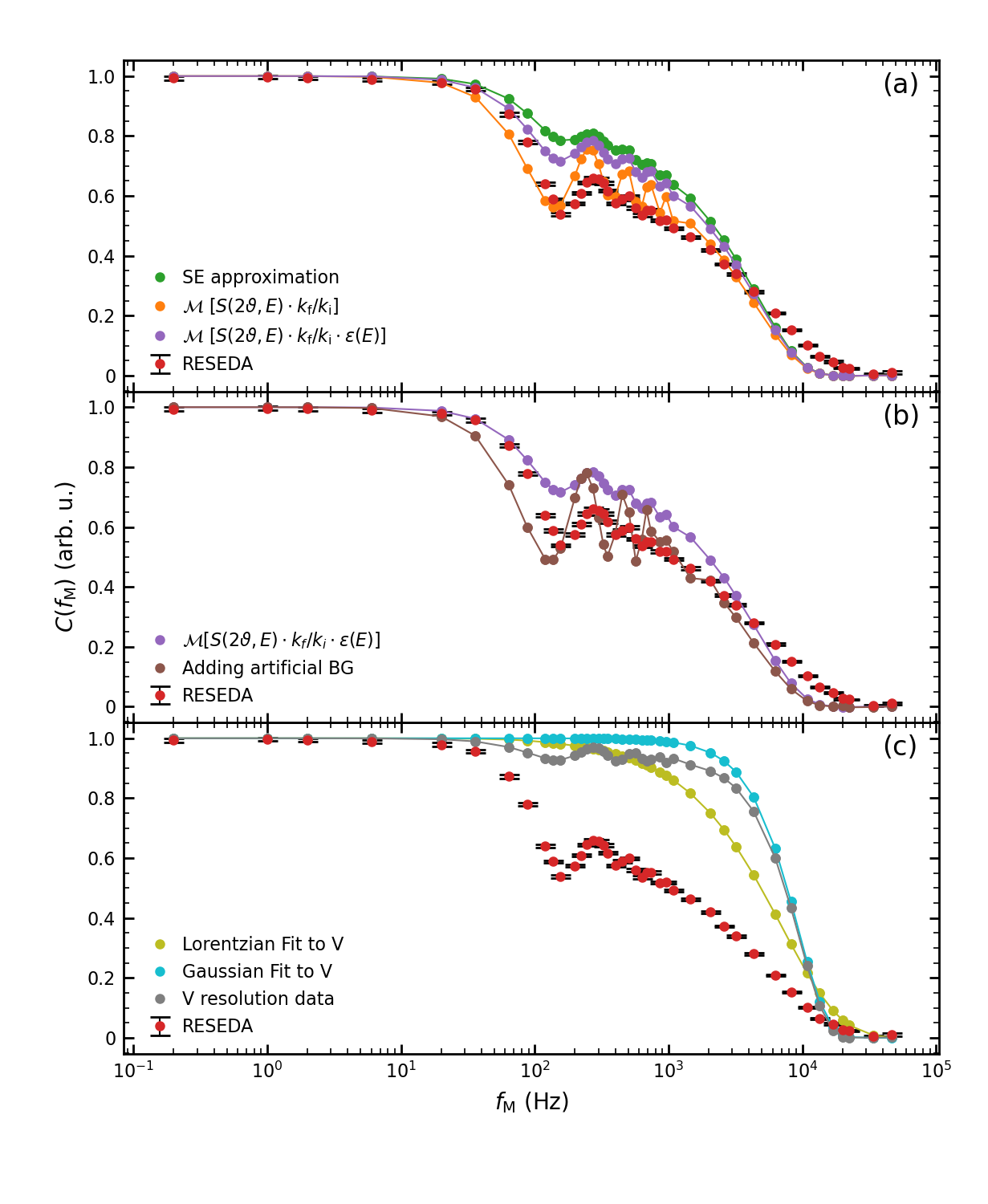
Figure 2: Direct transformation of TOFTOF $S(2\vartheta\!=\!$22\text{\,}\mathrm{\SIUnitSymbolDegree}$,E)$ data into the time domain. In (a) we show the transformed time-of-flight spectrum with increasing number of effects for direct comparison with the RESEDA data (red circles). The simplest case uses the spin-echo approximation (equation 9) and results in the green curve. The orange curve is obtained by transforming the energy spectrum with equation 18, which reproduces quite accurately the frequency of the oscillations visible in the RESEDA data. In purple, we have considered also the energy dependent detection efficiency of the CASCADE detector, which now accounts for the correct amplitude of the oscillations. Comparing the latter with the MIEZE data, at high frequencies the transformed ToF data decays faster and at medium frequencies the contrast is about $0.1$ higher than expected. Plot (b) visualizes the effect of introducing a constant background over the full energy range, leading to pronounced oscillations. In (c) we show the transformed resolution measurement of vanadium (gray) in comparison with a transformed Gaussian (turquoise) and Lorentzian (yellow) fit to the vanadium spectrum in energy space.

However, the exact numerical values of the MIEZE data can not be recovered, neither in the mid frequency nor in the high frequency range. Both discrepancies must be attributed to different origins, since the oscillations have been influenced by the introduction of $\varepsilon(E)$, whereas the faster decay at high $f_{\mathrm{M}}$ has been unaffected. Most notably this is true for the SE approximation as well.

The main source for the mismatch in the high frequency range is the fact that the TOFTOF data is convoluted with its resolution and it is not possible to disentangle the two for finite energy transfers. Empirical functions have been proposed [UNRUH2007] to describe the resolution, however they are not sufficient to fully disentangle the data from the resolution.
On the other hand, when transforming the MIEZE data into $Q-E$ space, the instrumental resolution of RESEDA only plays a minor role. Due to the properties of the Fourier transform the instrumental time resolution can easily be disentangled from the data by normalizing to the data of a purely elastic scatterer. However, due to the low data point density and the reduced sensitivity of MIEZE to inelastic signals, numerical artifacts need to be counteracted, and a regularization function is needed (analoguously to the transformation from reciprocal space to real space in SANS [bender2017structural]).
For the high frequency range however, the largest contribution to the mismatch between the RESEDA and TOFTOF data stems from the background measured at TOFTOF and its subsequent subtraction. Currently, no existing model describes the background over a large area in $Q$-$E$ space analytically or even empirically. Standard data treatment of ToF data includes the subtraction of a linear background. Consequently, this was done here as well. Varying this background by only 0.01% of the peak maximum leads to a significant variation in the Fourier transform of the data, as can be seen in figure 2. The origin of these effects will become more apparent in the next section and subsequently elaborated on in our discussion section 5

4.2 Combined fitting procedure using multiple Lorentzian distributions

A common approach to assess neutron data is the standard forward analysis, meaning that an idealized model function is hypothesized and subsequently compared with the data. Here, the baseline model is represented by a sum of Lorentzian distributions

$$S(2\vartheta,E)=\sum_{i}\frac{A_{i}}{\pi}\frac{\Gamma_{i}}{(E-E_{i})^{2}+\Gamma_{i}^{2}}~{},$$ (21)

where $2\Gamma_{i}$ is the linewidth (full width at half maximum), $E_{i}$ is either $0$ or a finite energy transfer and $A_{i}$ is the contribution of the excitation to the total dynamical structure factor, normalized to unity ($\sum_{i}A_{i}=1$).

Starting from this model, the data gathered on the pure water sample at $T=300\,\mathrm{K}$ by the ToF and MIEZE methods was analyzed via fitting of combined least-squares function. Fig. 3 summarizes the fitting process in a block diagram. The model treatment follows two distinct pathways for fitting the ToF and MIEZE data visualized as the blue and red boxes, respectively.

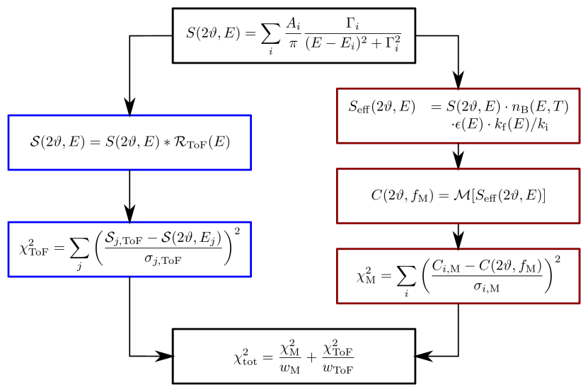
Figure 3: Flow chart of fitting the combined data set. Time-of-flight pathway is rimmed with blue boxes and the MIEZE pathway by dark red ones.

For a proper comparison between the reduced time-of-flight data and the Lorentzian sum model, the resolution function needs to be included. While the elastic linewidth can be readily measured using a vanadium reference sample, the resolution at finite energy transfers can only be estimated by mathematical models. In the case of the TOFTOF instrument, this has been explicitly studied by Unruh et al. [UNRUH2007] and Gaspar [2007Gaspar]. The main contributions to the uncertainty of the energy transfer have been identified to be the opening angles of the pulsing and monochromatizing choppers, as well as the detector tubes. The latter introduced uncertainty due to the detector’s dead time, flight time differences due to the geometry, and the wavelength dependent detection efficiency of the tubes. A scattering angle dependency was not included in the resolution function and has been neglected in this treatment.

The convolution of the baseline model with the TOFTOF resolution function was calculated as

$$\mathcal{S}(2\vartheta,E_{j})=\int\frac{1}{\sqrt{2\pi\sigma_{E_{j}}}}\exp{\left(\left[-\frac{E-E_{j}}{\sqrt{2}\sigma_{E_{j}}}\right]^{2}\right)}\cdot S(2\vartheta,E)\,\mathrm{d}E,$$ (22)

where $\sigma_{E_{j}}$ is the standard deviation expressing the instrumental uncertainty evaluated at the energy transfer $E_{j}$. Then, the least-squares function for the TOFTOF data $\chi^{2}_{\mathrm{ToF}}$ is computed (see fig. 3). For comparability, both, data set and convolution model are normalized to the area under $S(2\vartheta,E)$ respectively.

The analysis of the MIEZE data requires the transformation of the baseline model from the energy domain into the time domain. Especially in the case of large energy transfers, this requires to compute the contrast via equation 18. For the baseline model to adhere to the theoretical framework laid out above, the detailed balance factor $n_{\mathrm{B}}(E,T)=\exp{\left(-E/k_{\mathrm{B}}T\right)}$, the detector efficiency $\epsilon(E)$ and the correction factor $k_{\mathrm{f}}(E)/k_{\mathrm{i}}$ need to be multiplied to the model of the dynamic structure factor. This is indicated in the upper red box of fig. 3. Subsequently, we calculate the transformation, denoted by $\mathcal{M}[\cdots]$, using the effective structure factor ($S_{\mathrm{eff}}(2\vartheta,E)$) in 18 and computing the least-squares value of the MIEZE data $\chi^{2}_{\mathrm{M}}$.

Summing up both $\chi^{2}_{\mathrm{X}}$ ($\mathrm{X}=\text{ToF, M}$) values yields the total least-squares value $\chi^{2}_{\mathrm{tot}}$, which ought to be minimized by the optimal model through variation of the free parameters, $A_{i}$, $E_{i}$ and $\Gamma_{i}$ of each Lorentzian peak. However, adding up the $\chi^{2}$ values is not straightforward. Due to the comparably large number of data points and the smaller relative uncertainty, $\chi^{2}_{\mathrm{ToF}}$ dominates the combined least-squares function. While this will be discussed in more detail later, especially in context of the uncertainty estimates, we have opted to weight $\chi^{2}_{\mathrm{X}}$ by $1/N_{\mathrm{X}}$, with $N_{\mathrm{X}}$ being the number of data points.

Numerical optimization was done utilizing the differential evolution algorithm [storn1997differential] implemented in the scipy [2020SciPy-NMeth] library as well as the Python wrapper package iminuit, which makes the MIGRAD algorithm of CERN’s ROOT data analysis framework available [dembinski_iminuit_2020, antcheva_root_2011]. The uncertainty of the obtained fit parameters have been evaluated using the inverse Hessian matrix and population statistics acquired by differential evolution fitting, which is explained in more detail in appendix A.

4.2.1 Two quasielastic and one inelastic contribution (2Q1I)

The shape of the TOFTOF data and modeling in literature [AmannWinkel2016] hint that a heuristic model comprises two quasielastic and one inelastic Lorentzian contributions to parameterize $S(2\vartheta,E)$. This accounts for the rotational and translational diffusion of water, as well as the inelastic peak observed at $E\approx 50\,\mathrm{meV}$. This high energy transfer changes the neutron wavelength to $\simeq\,1.3\,$Å, which results in a wavevector transfer of $\simeq\,3.9\,\mathrm{\AA^{1}}$ (for $2\vartheta\,=\,22^{\circ}$), which would probe the libration of the OH-bonds. Due to the dominating incoherent scattering length of $\mathrm{H}_{2}\mathrm{O}$, collective phenomena such as fast sound are not resolvable. They are expected to appear at low $Q$ ($<$1\text{\,}\mathrm{\SIUnitSymbolAngstrom}$$) having $6\text{\,}\mathrm{meV}10\text{\,}\mathrm{meV}$.

As a first step, which generally has been performed for each of the following models, the fit result of the TOFTOF data alone, was used as a starting point for further combined fitting. The result of fitting only the ToF data is tabulated in table 1. Here, we list the uncertainty estimates of the standard Hesse approach and of the population statistics for a $2\text{\,}\%$ deviation from the minimum $\chi^{2}_{\mathrm{X}}$, which yields comparable uncertainties and can be considered an adequate estimate, whenever the Hesse approach is not viable.

Table 1: Results of the 2 QENS + 1 INS model (2Q1I) to the ToF data. The uncertainties shown here have been estimated either by a quadratic approximation of the respective $\chi^{2}_{\mathrm{X}}$ function (Hesse) or via the standard deviation of the differential evolution population (Population) within the $2\text{\,}\mathrm{\char 37\relax}$ threshold.

	ToF	Hesse	Population
$\Gamma_{1}$ (meV)	$0.0327$	$0.0004$	$0.0005$
$A_{1}$	$0.7711$	$0.0051$	$0.0047$
$\Gamma_{2}$ (meV)	$4.5621$	$0.1139$	$0.1499$
$A_{2}$	$0.2071$	$0.0027$	$0.0038$
$\Gamma_{3}$ (meV)	$14.588$	$0.573$	$0.875$
$E_{3}$ (meV)	$50.107$	$0.8624$	$1.2787$
$A_{3}$	$0.0171$	$0.0007$	$0.0001$
$\chi^{2}_{\mathrm{ToF}}$	40.1

A graphical representation for the fitting results of the ToF, MIEZE and combined fit are given in figures 4 and 5. While the former graphic shows the comparison between model and the data, the latter visualizes the fit parameters of the 2Q1I model as they are extracted from each data set.

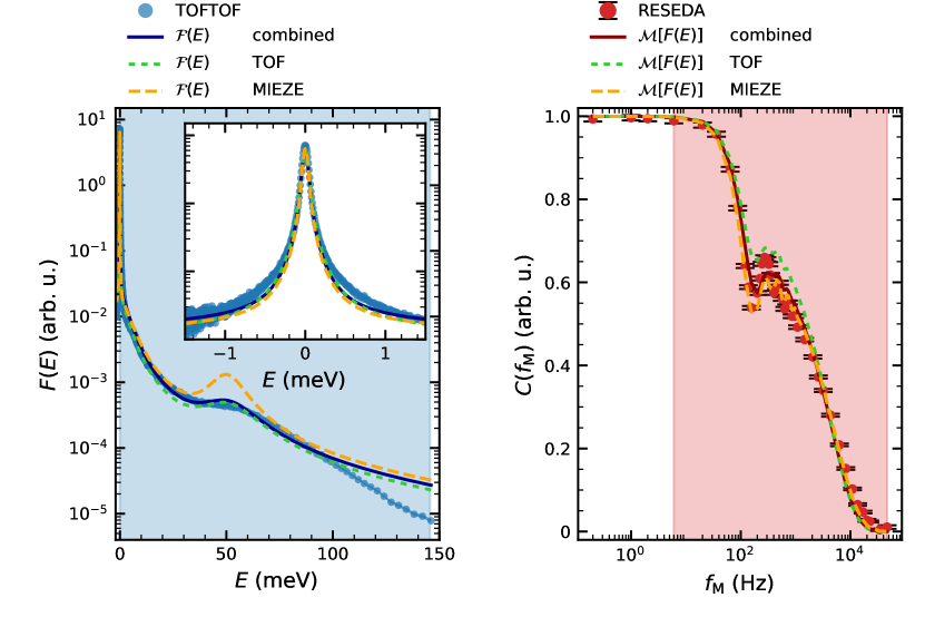
Figure 4: Result of fitting the 2Q1I model. The points in blue or red visualize the measurement of TOFTOF and RESEDA, respectively. Wherever errorbars are missing, they would significantly smaller then the size of the markers. The solid lines represent the result of the combined fit analysis. The dashed orange line represents the fit of the RESEDA data and has been convolved with the instrument resolution for comparison with the TOFTOF data. Similarly, the green, dotted line visualizes the fit of the TOFTOF data and has been transformed for comparison with the RESEDA data. The fit of the MIEZE data is insensitive to the inelastic scattering contribution, which is why the amplitude is overestimated too improve the at low energy transfers.

In case of the TOFTOF data, the uncertainty of each point is smaller than the marker size, which is why it has been omitted in the plot. The error bars of the RESEDA data represent the purely statistical uncertainty of the contrast value, as it is retrieved from the data reduction of MIEZEPY (see section 3.1). The result of three fits have been visualized, where the solid (blue and dark red) lines denote the combined fit, the green, broken line, represents a fit to the TOFTOF data only and the golden, dash-dotted line visualizes the result of solely fitting the RESEDA data. For both fits of a single data set, the resulting $S(2\vartheta,E)$ was processed for comparison with the second data set. Several observation can be made from figure 4. (i) The 2Q1I model does not describe the ToF data in the medium ($0.4\text{\,}\mathrm{meV}1.0\text{\,}\mathrm{meV}$) and large ($>$100\text{\,}\mathrm{meV}$$) energy transfer region. In the former, it underestimated $S(2\vartheta,E)$ while it overestimates the decaying dynamical structure factor in the latter. (ii) The fit involving both data sets interpolates both individual fit results. (iii) The MIEZE data has no sensitivity to the large energy transfer inelastic contribution to the observed contrast. The inelastic contribution ought to appear in the $3$ to $4$ MIEZE data points around the contrast drop at $1.0\text{\times}{10}^{-4}\text{\,}\mathrm{ns}$. However, since its relative weight to the total dynamical structure factor is $\approx$2\text{\,}\%$$, the corresponding contrast variation is on the order of the statistical uncertainty of the measurement. As a result, a unconstrained fit of the 2Q1I model to the RESEDA data converges to a model comprising of three superimposed quasielastic distributions. For this reason, we analyzed the RESEDA data with a model, where $E_{\mathrm{I1}}=$50.1\text{\,}\mathrm{meV}$$ was fixed. This value is the result of the ToF fit.

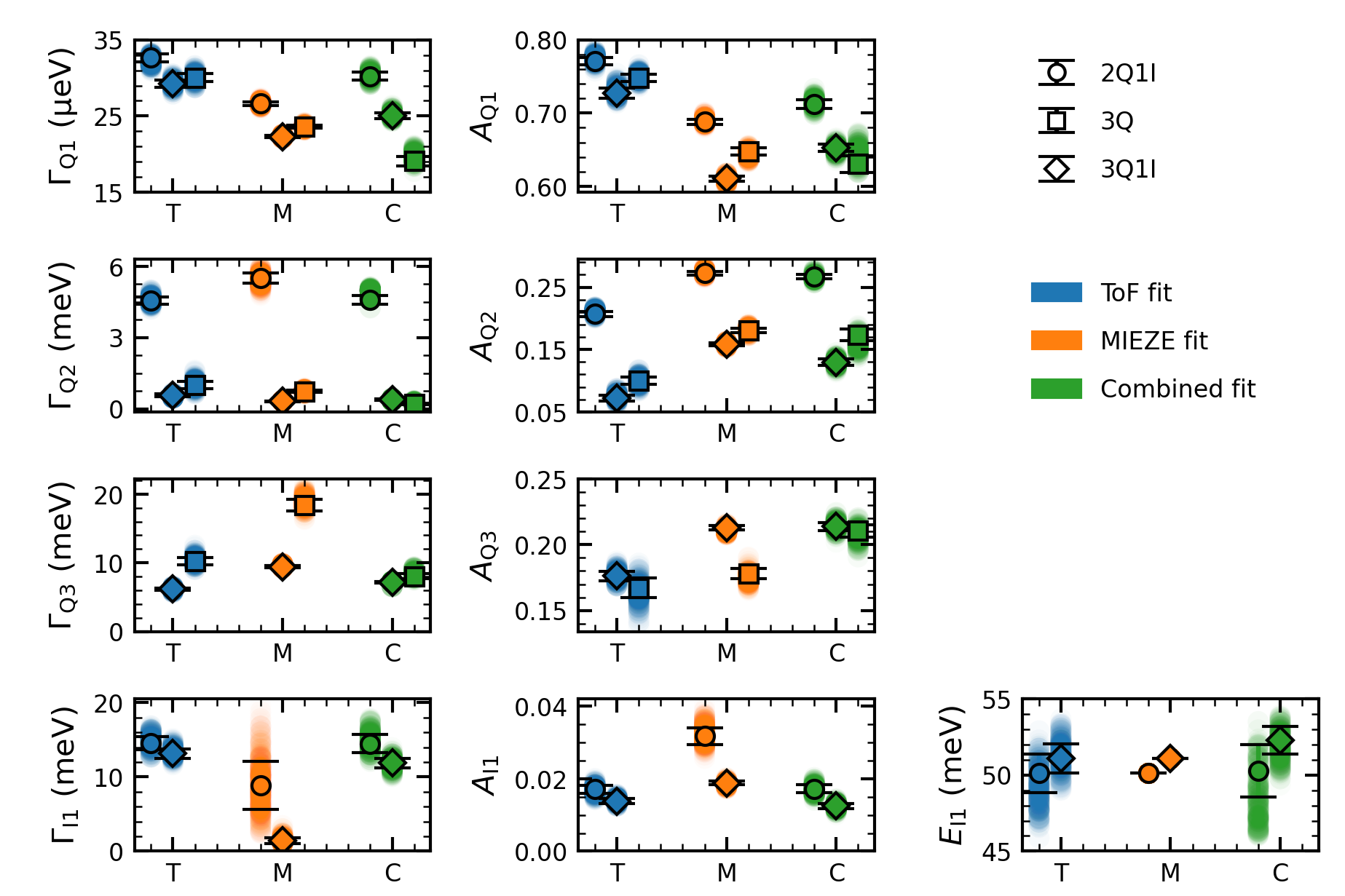
Figure 5: Summary of the model fit approach of the ToF and MIEZE data. The markers indicate the model, while the color encodes the data set which was analyzed using a particular model. The shaded area below a marker visualizes the distribution in this parameter which satisfies the $2\text{\,}\mathrm{\char 37\relax}$ deviation from minimum $\chi^{2}_{\mathrm{X}}$ criterion. The errorbar of each marker represents the standard deviation of that distribution. Note that $E_{\mathrm{I1}}$ was fixed when fitting the MIEZE data.

4.2.2 Three quasielastic contributions (3Q)

As a consequence of the insensitivity of the MIEZE method to large energy transfers, we now limit the employed fitting model to three quasielastic distributions (3Q model). It is evident from figure 5, that there is a significant change in $\Gamma_{\mathrm{Q2}}$, as there is an additional quasi-elastic distribution to fit the large energy transfer data. Furthermore, this leads to a, positive correlation between the $\Gamma_{\mathrm{Q1}}$ and $A_{\mathrm{Q1}}$ because the narrow distribution needs to fit the low energy transfer data, while simultaneously needing to account for less spectral weight at high energy, as compared to the 3Q or 3Q1I model. In addition, the drastic improvement of the $g_{\mathrm{fit,M}}$ (see table 2) for the 3Q model justifies the introduction of a third quasielastic contribution to $S(2\vartheta,E)$.

4.2.3 Three quasielastic and one inelastic contribution (3Q1I)

An inherent problem to this modeling approach is the introduction of unnecessary fit parameters and overfitting, as an unlimited number of Lorentzian distributions can easily be fitted to the data. Given the fact that the 3Q model leads to a significant improvement over 2Q1I in the region $-1\text{\,}\mathrm{meV}1\text{\,}\mathrm{meV}$ and that one inelastic component in the ToF spectrum is evident, it stands to reason that a 3Q1I model should be analyzed. Again for the MIEZE fit the $E_{\mathrm{I1}}$ was fixed to the previous value determined from the ToF data.

The $g_{\mathrm{fit,X}}$ values reduce further to their lowest value, as indicated by table 2. In comparison with the 3Q model, the parameters of the two narrow distributions change only marginally, as this part of the data is already well described by both models. Larger variations can be seen in the parameters of the Lorentzian distribution $L_{\mathrm{Q3}}$ as the inelastic distribution $L_{\mathrm{I1}}$ adds descriptive power in the high energy transfer regime. Same as in model 2Q1I, the MIEZE data is not sensitive in this regime, which is why the fit parameters of $L_{\mathrm{Q3}}$ and $L_{\mathrm{I1}}$ vary and are subject to large uncertainty.

Table 2: Summary of the $g_{\mathrm{fit,X}}$ parameters for every combination of data set and model.

$g_{\mathrm{fit,X}}$	ToF	MIEZE	Combined
2Q1I	$40.1$	$30.2$	$56.8$
3Q	$58.9$	$8.8$	$47.6$
3Q1I	$31.1$	$3.3$	$35.8$

Even though some parts in the evolution of the fit parameters from model 2Q1I to 3Q and to 3Q1I can be explained by the general structure of the data in relation to these models, systematic differences arise especially in the parameter values obtained by fitting ToF and MIEZE data separately. As an example, the ToF fit estimates $\Gamma_{\mathrm{Q1}}$ to be about $30\text{\,}\mathrm{\char 37\relax}$ higher than the MIEZE fit. Similar deviations can be observed in $A_{\mathrm{Q1}}$, $\Gamma_{\mathrm{Q2}}$ and $A_{\mathrm{Q2}}$. We will connect these discrepancies with the problems identified in the direct transformation approach in the discussion section hereafter.

5 Discussion

We have introduced an analytical framework with which the MIEZE contrast can be calculated beyond the SE approximation and we have subsequently used this formalism to compare data measured at the time-of-flight spectrometer TOFTOF with data measured at the MIEZE spectrometer RESEDA under the same experimental conditions. The analysis requires a deep understanding of the instrumental resolution functions of TOFTOF and the efficiency of the CASCADE detector to achieve comparability of the data and fit parameters. Nevertheless, discrepancies remain.

First, we focus on the difference in the fit parameter $\Gamma_{\mathrm{Q1}}$ of the narrowest Lorentzian distribution in energy space that corresponds to the slowest contrast decay in the Fourier time domain. It is apparent in figure 2 (a) that the direct transformation of the energy spectrum decays faster than the MIEZE data. In energy space, this corresponds to a broader peak, which we attribute to the limited instrumental resolution of the ToF instrument around the elastic line. This, can not be corrected before performing the transformation from energy to time domain, as an inverse convolution is a mathematically ill defined problem. Approximations of the measured resolution function using a Gaussian or Lorentzian are insufficient to describe the necessary details (as shown in figure 2 (c) by the yellow and turquoise points in comparison to the grey ones). This becomes problematic as the model of the TOFTOF resolution is not able to fully account for the broadening of the elastic line. Comparing the calculated resolution at $E=0$ with the experimentally determined resolution of a standard vanadium sample fitted with a Gaussian, we found: $\sigma_{\mathrm{calc}}=$17.6\text{\,}\mathrm{\SIUnitSymbolMicro eV}$$ and $\sigma_{\mathrm{exp}}=$20.7\text{\,}\mathrm{\SIUnitSymbolMicro eV}$$. Hence, the fit of the ToF data using the calculated energy resolution function, overestimates the linewidth $\Gamma_{\mathrm{Q1}}$. To correct for this overestimation, we can use an estimate of the FWHM $f_{\mathrm{V}}\approx 0.5346\cdot 2\Gamma+\sqrt{0.2166\cdot(2\Gamma)^{2}+8\ln{(2)}\cdot\sigma^{2}}$ of a Voigt profile, which is a convolution of a Lorentzian distribution with a Gaussian resolution function. Using this, the corrected values become:

• 2Q1I: $32.7\text{\,}\mathrm{\SIUnitSymbolMicro eV}$ $\longrightarrow$ $28.8\text{\,}\mathrm{\SIUnitSymbolMicro eV}$

• 3Q: $30.0\text{\,}\mathrm{\SIUnitSymbolMicro eV}$ $\longrightarrow$ $25.9\text{\,}\mathrm{\SIUnitSymbolMicro eV}$

• 3Q1I: $29.2\text{\,}\mathrm{\SIUnitSymbolMicro eV}$ $\longrightarrow$ $25.0\text{\,}\mathrm{\SIUnitSymbolMicro eV}$

While this does not account for the entire difference between the MIEZE and ToF fit, it cuts down the relative difference from $21\text{\,}\mathrm{\char 37\relax}$ to $9\text{\,}\mathrm{\char 37\relax}$, which can be better reconciled with the uncer s.

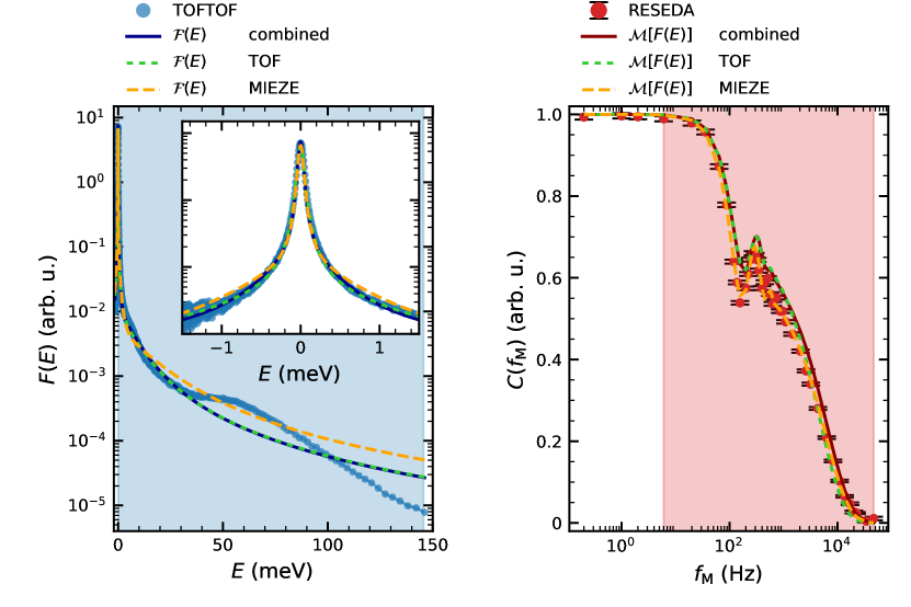
Figure 6: Result of fitting the 3Q model. The plot format follows the same style as fig. 4. The 3Q model fit improves the low $E$ description of the spectrum, while it, by construction, neglects the inelastic part that is necessary to adequately model the ToF data.

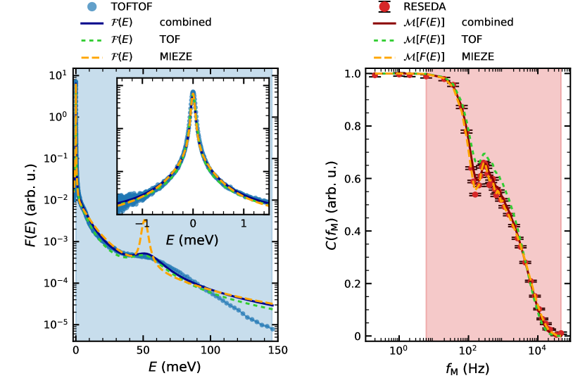
Figure 7: Result of fitting the 3Q1I model. The plot format follows the same style as fig. 4.

The second issue relates to the differing weights $A_{i}$ of the distributions $Q1$ and $Q2$, when comparing the fits of the ToF and MIEZE data. In the case of $Q1$ this can be attributed to the positive correlation between $\Gamma$ and $A$. Meaning that an overestimation of $\Gamma_{\mathrm{Q1}}$ by the ToF fit, leads also to a larger value of $A_{\mathrm{Q1}}$ and is corrected by considering the experimental resolution as described above. For energy transfers in the range of $1.0\text{\,}\mathrm{meV}25.0\text{\,}\mathrm{meV}$, which correspond to about $100\text{\,}\mathrm{Hz}1000\text{\,}\mathrm{Hz}$ in figure 2, we attribute the discrepancy in contrast between both data sets to the insufficient modeling of the detector efficiencies as a function of energy transfer. The origin cannot be discerned from the present data, but the ToF data underestimates the relative contribution to $S(2\vartheta,E)$ at high energy transfer compared to the MIEZE data. This notion is further substantiated by looking at the fits of the models in comparison to the energy spectrum in figures 4, 6 and 7. Spurious, inelastic scattering at such high energy transfers cannot be ruled out, but seems to be an unrealistic root cause. Thirdly, the dark count rate of the TOF-detectors turned out to be a crucial parameter. Dark counts are equally distributed over the time bins and appear as a constant background along the resolved energy band. These finite values at the edges of the Fourier-transform window alter the oscillations amplitude in the time domain drastically, as shown in figure 2 b).

Another explanation for the mismatch of the models in energy space is the assumption of using simple Lorentzian distributions. In the context of critical phenomena, correlation functions are known to assume more complex shapes. Due to the sensitivity of the MIEZE method to the flanks of $S(2\vartheta,E)$ appropriate model functions are required to extract the correct, physical parameters from the data [boni_comparison_1993, beddrich2023consequences]. Moreover, the $\chi^{2}$-analysis of the combined fit of TOFTOF and RESEDA data proved challenging due to the large difference in the number of data points and therefore statistical significance of the two datasets. Without aforementioned normalization the fit will only take into account the TOFTOF data since it contains many more data points ($N_{\mathrm{ToF}}\approx$700$$, $N_{\mathrm{M}}=$42$$). However, the normalization distorts the $\chi^{2}$ - landscape creating a minimum, where optimal values of the fit parameters lie outside the expected parameter space spanned by fitting the ToF and MIEZE data individually, as shown in figure 5, where $\Gamma_{\mathrm{2,C}}\notin[\Gamma_{\mathrm{2,M}};\Gamma_{\mathrm{2,T}}]$, e.g. green sqares in the $\Gamma_{\mathrm{Q1}}$ plot. It is therefore not viable to analyze the combined fit in a $\chi^{2}$ framework, as long as the statistic significance of the data set is considerably imbalanced and the aforementioned instrument performance is insufficiently characterized.

6 Conclusion

In conclusion, we have presented several data analysis approaches to compare MIEZE and ToF data. While the agreement between the datasets is reasonably good, we have found several instrumental details that play an essential role in this comparison, some of which need to be taken into account with great care, such as detector efficiencies, uncharacterized backgrounds and dark counts.

This study highlights the complementarity of MIEZE and ToF and the necessity of making data collected with these techniques more comparable. Where MIEZE offers significantly higher energy resolution, ToF does provide a larger section of Q-E space in a shorter measurement time. And while MIEZE is ideally suited to study dynamic processes at small scattering angles TOF can more easily discern dynamics at large energy transfers.

The comparability of these two techniques might be aided by computational physics methods such as molecular dynamics simulations which allow the extraction of the dynamical structure factor from the trajectories of a large ensemble of molecules, which can improve the models used when comparing the data using the approach discussed here.

Additionally, we want to emphasize that the explicit expression for the MIEZE contrast, which we used here to translate the ToF measurement into the MIEZE contrast and vice versa, holds true in general for NSE. While we understand that the SE approximation results in the nice and compact relation between the two parameter spaces via a simple cosine Fourier transform, there is no real need to apply such a simplification when translating one into the other.

7 Acknowledgements

This manuscript has benefited immensely from discussions with many of the authors’ co-workers. Among them are: Thomas Keller, Olar Holderer, Macell Wolf, Wiebke Lohstroh, and Sebastian Busch. The authors further want to acknowledge financial support through the BMBF projects ‘Longitudinale Resonante Neutronen Spin-Echo Spektroskopie mit Extremer Energie-Auflösung’ (Förderkennzeichen 05K16W06) and ’Resonante Longitudinale MIASANS Spin-Echo Spektroskopie an RESEDA’ (Förderkennzeichen 05K19W05).

Appendix A Uncertainty analysis

For the fitting using only one single data set, we can use the common uncertainty estimation, by a quadratic approximation of the least-squares cost function around the minimum. For the least-squares analysis, the $1\sigma$ uncertainty estimate and covariance of a fit parameter $a_{i}$ is given by the contour in parameter space, where the $\chi^{2}=\chi^{2}_{\mathrm{min}}+1$. This contour can be traced out by mapping out the least-squares cost function around the minimum, which becomes exceedingly time consuming in cases of a high dimensional fit parameter space. More efficient is the calculation of a quadratic approximation of the least-squares function using the Hessian matrix used in gradient descent or related minimization algorithms. The standard uncertainty of a fit parameter $a_{i}$ is then calculated as $\sigma_{a_{i}}=\left(\mathbf{H}^{-1}\right)_{ii}$. Ideally, the fit of an appropriate model function to a set of data points and their standard deviation $(y_{i},\sigma_{i})$ should result in a goodness-of-fit value $g_{\mathrm{fit}}\approx 1$, which is calculated as

$$g_{\mathrm{fit}}=\frac{1}{n-m}\sum^{n}_{i}w_{i}\cdot\left[f(x_{i}|\mathbf{a})-y_{i}\right]^{2}~{},$$ (23)

similar to the reduced $\chi^{2}$ value. However, the $\sigma_{i}$ values do not necessarily capture all uncertainty associated with the value $y_{i}$ leading to a $g_{\mathrm{fit}}$ significantly larger than $1$. $n$ is the number of data points and $m$ is the number of fit parameters included in the model function $f$. In a first attempt to account for this fact, $g_{\mathrm{fit}}$ can be used as a scaling factor between the weights in the least-squares function $w_{i}$ and the $\sigma_{i}$ associated with each data point: $w_{i}=g_{\mathrm{fit}}/\sigma_{i}^{2}$. Then, $\sigma_{i}$ represent relative uncertainties between the data points, but not the ’total uncertainty’. As a result, the uncertainties of the fit parameters need to be re-scaled to $\sigma_{a_{i}}^{2}=g_{\mathrm{fit}}\cdot\left(\mathbf{H}^{-1}\right)_{ii}$ as well.

The method to estimate the reliability of the fit parameters assumes certain statistics of the data points used in the computation of the $\chi^{2}$ value. In case of the combined model with $\chi^{2}_{\mathrm{tot}}$, the unnatural emphasis of the MIEZE data skews the results compared to a standard least-squares function. Thus, besides the uncertainty estimates obtained from the calculations described above, we used the intermediate results of the differential evolution algorithm to study the distribution of fit parameters, which yielded $\chi_{\mathrm{tot}}^{2}\leq\chi^{2}_{\mathrm{tot,min}}\cdot 1.02$. The populations of vectors in parameter space, which are drawn by the differential evolution algorithm, have been produced via the best1bin strategy [storn1997differential]. The uncertainty of each optimal parameter is then determined by calculating the standard deviation of the marginalized distribution with respect to the optimal value. For a $2\text{\,}\%$ deviation from the minimal $\chi^{2}$ between $200$ and $400$ parameter vectors are used for this analysis.

Appendix B Fit results

[Bib]