Posterior Ramifications of Prior Dependence Structures

Abstract

In fully Bayesian analyses, prior distributions are specified before observing data. Prior elicitation methods transfigure prior information into quantifiable prior distributions. Recently, methods that leverage copulas have been proposed to accommodate more flexible dependence structures when eliciting multivariate priors. The resulting priors have been framed as suitable candidates for Bayesian analysis. We prove that under broad conditions, the posterior cannot retain many of these flexible prior dependence structures as data are observed. However, these flexible copula-based priors are useful for design purposes. Because correctly specifying the dependence structure a priori can be difficult, we consider how the choice of prior copula impacts the posterior distribution in terms of convergence of the posterior mode. We also make recommendations regarding prior dependence specification for posterior analyses that streamline the prior elicitation process.

Keywords: Copulas; design and analysis of experiments; prior elicitation; the Bernstein-von Mises theorem

1 Introduction

1.1 Brief Overview of Prior Elicitation

Statistical methods leverage data to infer properties about an unobservable, possibly multivariate parameter $\boldsymbol{\theta}=(\theta_{1},...,\theta_{d})$. Bayesian methods for statistical inference (see e.g., (Gelman et al., 2013)) require the specification of a prior distribution for the parameter $\boldsymbol{\theta}$, denoted by $p(\boldsymbol{\theta})$. This distribution characterizes the beliefs about $\boldsymbol{\theta}$ prior to observing any data. For a particular statistical model, $L(\boldsymbol{\theta};\hskip 1.0pt\boldsymbol{y})$ is the relevant likelihood function for the parameter $\boldsymbol{\theta}$ with respect to the observed data, denoted by the vector or matrix $\boldsymbol{y}$. Bayesian inference employs Bayes’ theorem to update the beliefs about the random variable $\boldsymbol{\theta}$ as more information becomes available via the observed data. In the Bayesian paradigm, inference is facilitated via the posterior distribution of $\boldsymbol{\theta}$, denoted by $p(\boldsymbol{\theta}\hskip 1.0pt|\hskip 1.0pt\boldsymbol{y})$. This distribution communicates which values of $\boldsymbol{\theta}$ are plausible given the observed data and prior beliefs. By Bayes’ Theorem, we have that

$$p(\boldsymbol{\theta}\hskip 1.0pt|\hskip 1.0pt\boldsymbol{y})=\dfrac{L(\boldsymbol{\theta};\hskip 1.0pt\boldsymbol{y})\hskip 1.0ptp(\boldsymbol{\theta})}{\int L(\boldsymbol{\theta};\hskip 1.0pt\boldsymbol{y})\hskip 1.0ptp(\boldsymbol{\theta})d\boldsymbol{\theta}}\propto L(\boldsymbol{\theta};\hskip 1.0pt\boldsymbol{y})\hskip 1.0ptp(\boldsymbol{\theta}).$$ (1)

To implement fully Bayesian analyses, prior distributions must be specified before observing data. This is in contrast to empirical Bayes methods that set the parameters for the prior distributions to their most likely values given the observed data (Casella, 1985; Carlin and Louis, 2000). In the absence of prior information, uninformative or diffuse priors are often used. When relevant prior information from subject matter experts or previous statistical analyses is available, it rarely takes the form of quantifiable prior distributions on the unobservable parameters of a statistical model. Prior elicitation procedures are used to transfigure prior information into quantifiable prior distributions.

Winkler (1967) conducted some of the initial work on prior elicitation, citing the siloed nature of prior specification and posterior analysis. Most previous Bayesian research had investigated how to leverage sample information from the likelihood function to obtain the posterior from the prior distribution, which was assumed to have been already assessed. Winkler (1967) explored four elicitation methods for Bernoulli processes, two of which involved directly asking questions about the prior cumulative distribution function (CDF) or probability distribution function (PDF) for the Bernoulli parameter. The two remaining methods indirectly extracted participants’ prior beliefs about the Bernoulli parameter using hypothetical binomial samples. These elicitation methods were for univariate priors, yet Winkler (1967) acknowledged that the assessment of prior distributions in multivariate contexts was an important and nontrivial problem.

Decades later, Chaloner (1996) overviewed methods for subjective prior specification with an emphasis on methods for clinical trials. In this context, Freedman and Spiegelhalter (1983) elicited a prior on the difference in cancer recurrence probability between treatment groups by asking experts about the mode and likely lower and upper bounds for this difference. This prior was not combined with observed data and instead used to choose the number of interim analyses in a sequential design. In clinical trials, it is not uncommon to use a prior distribution solely for design purposes, such as determining whether random treatment assignment is ethical (Errington et al., 1991). Other contributions in clinical settings advocated for soliciting prior beliefs from several experts to form a community of prior distributions and basing inference on a consensus of posterior conclusions (Kadane, 1986; Chaloner et al., 1993). Most prior elicitation methods overviewed by Chaloner (1996) considered more complex models than the univariate Bernoulli process in Winkler’s (1967) initial work. To reduce cognitive and computational complexity, many of these methods relied on parametric assumptions and solicited information about potentially observable conduits for the unobservable parameter $\boldsymbol{\theta}$ that are easier to conceptualize. For instance, priors for Bayesian regression model coefficients were elicited using information about quantiles of predictive distributions (Kadane et al., 1980) and survival probabilities (Chaloner et al., 1993).

Additional reviews of prior elicitation methods have since been conducted. Garthwaite et al. (2005) divided the elicitation process into four stages: setup, elicitation, fitting, and adequacy. These stages involve preparing the expert for elicitation, eliciting distributional summaries of expert knowledge, fitting a probability distribution to these summaries, and assessing the adequacy of elicitation. O’Hagan et al. (2006) focused on elicitation of subjective probabilities and noted that experts tend to characterize events as impossible instead of assigning small probabilities to them. Because this gives rise to hard and potentially unrealistic boundaries in the support of the elicited priors, O’Hagan et al. (2006) overviewed methods to correct for expert overconfidence. Johnson et al. (2010) conducted a systematic review of prior elicitation methods with an emphasis on the feasibility of the process in terms of the required time, cost, personnel, and equipment. They found that although expert fatigue and lack of understanding compromise the reliability of elicitation procedures (Winkler, 1971; Garthwaite et al., 2005), the reviewed methods were rarely formally evaluated on their feasibility.

Recent contributions have aimed to reduce expert fatigue and improve understanding by developing iterative elicitation procedures that provide experts with instant feedback via a graphical interface (Jones and Johnson, 2014; Casement and Kahle, 2018; Williams et al., 2021; Casement and Kahle, 2023). Prior elicitation procedures have also been developed for more complex settings – including methods for rank analysis (Crispino and Antoniano-Villalobos, 2023), nonparametric models (Seo and Kim, 2022), sequential analysis (Santos and Costa, 2019), power priors (Ye et al., 2022), and mixture models (Fúquene et al., 2019; Feroze and Aslam, 2021). One such area of research involves using copulas to accommodate more flexible dependence structures when eliciting multivariate priors (Elfadaly and Garthwaite, 2017; Wilson, 2018; Wilson et al., 2021). These contributions are novel given that the dependence structure is an afterthought in many recent prior elicitation methods. In particular, many recent methods consider elicitation for univariate parameters (Casement and Kahle, 2018, 2023), fix the dependence structure to leverage conjugacy (Santos and Costa, 2019; Srivastava et al., 2019), or assume that the components of $\boldsymbol{\theta}$ are independent a priori (Garthwaite et al., 2013; Jones and Johnson, 2014; Fúquene et al., 2019; Seo and Kim, 2022). Prominent recent advances with copula-based priors are overviewed in Section 1.2.

1.2 Recent Developments with Copula-Based Priors

Copulas allow for more flexible dependence structures when eliciting multivariate distributions. The behaviour of random variables $\boldsymbol{X}=\{X_{1},X_{2},...,X_{d}\}$ is often characterized by their joint distribution function $H(\boldsymbol{x})$. Each component of $\boldsymbol{X}$ also has a marginal distribution function $F_{j}(x_{j})=Pr(X_{j}\leq x_{j}),~{}j=1,...,d$. Copulas allow for the dependence structure of $\boldsymbol{X}$ to be considered separately from its marginal distributions. Let $U_{1},U_{2},...,U_{d}$ be uniformly-distributed random variables over the unit interval $[0,1]$. The distribution function

$$C(u_{1},...,u_{d})=Pr(U_{1}\leq u_{1},...,U_{d}\leq u_{d})$$

is such that $C:[0,1]^{d}\rightarrow[0,1]$ is a copula (Nelsen, 2006). Sklar’s theorem (Sklar, 1959; Schweizer and Sklar, 2011) explicates the relationship between the copula $C$, the multivariate joint distribution function $H(\boldsymbol{x})$, and the univariate marginal CDFs $F_{j}(x_{j})$ for $j=1,...,d$:

$$H(\boldsymbol{x})=C(F_{1}(x_{1}),...,F_{d}(x_{d})),$$

where $\boldsymbol{x}=(x_{1},...,x_{d})\in\mathcal{X}\subseteq\mathbb{R}^{d}$. If $F_{1},...,F_{d}$ are continuous, then the copula $C$ is unique.

A copula $C$ can be represented as the sum of its absolutely continuous component $A_{C}$ and singular component $S_{C}$ (Nelsen, 2006). That is, $C(\boldsymbol{u})=A_{C}(\boldsymbol{u})+S_{C}(\boldsymbol{u})$, where $\boldsymbol{u}=(u_{1},...,u_{d})\in[0,1]^{d}$ and

$$A_{C}(\boldsymbol{u})=\int_{0}^{u_{1}}\cdots\int_{0}^{u_{d}}\dfrac{\partial^{d}}{\partial t_{1}\cdots\partial t_{d}}C(t_{1},...,t_{k})dt_{k}\cdots dt_{1}.$$

If $C=A_{C}$ on $[0,1]^{d}$, then the copula $C$ is absolutely continuous and admits a density function

$$c(\boldsymbol{u})=\dfrac{\partial^{d}}{\partial u_{1}\cdots\partial u_{d}}C(u_{1},...,u_{d}).$$

Moreover, if the support of $C$ is $[0,1]^{d}$, then the copula is deemed to have full support (Nelsen, 2006).

Copulas can be defined using common probability distributions. For instance, the Gaussian copula (Clemen and Reilly, 1999) with correlation matrix $\boldsymbol{R}$ is defined such that

$$C^{Ga}_{\boldsymbol{R}}(\boldsymbol{u})=\Phi_{\boldsymbol{R}}(\Phi^{-1}(u_{1}),...,\Phi^{-1}(u_{d})),$$

where $\Phi$ is the CDF of the $\mathcal{N}(\boldsymbol{0},1)$ distribution and $\Phi_{\boldsymbol{R}}:\mathbb{R}^{d}\rightarrow[0,1]$ is the CDF of the $d$-dimensional $\mathcal{N}(\boldsymbol{0},\boldsymbol{R})$ distribution with correlation and covariance matrix $\boldsymbol{R}$. The $t$-copula (Demarta and McNeil, 2005) can be similarly defined given a multivariate $t$-distribution with correlation matrix $\boldsymbol{R}$ and degrees of freedom $\nu$. In contrast, Archimedean copulas are a commonly used class of copulas that are efficiently parameterized via generator functions (Nelsen, 2006).

Copulas can be incorporated into the prior elicitation process as illustrated in recent developments for the multinomial model. Elfadaly and Garthwaite (2017) proposed one such method to elicit Gaussian copula prior distributions. The standard multinomial model assumes that data $y_{i}\in\{1,2,...,w\},~{}i=1,...,n$ are collected independently and that the outcome $v$ occurs with probability $0<p_{v}<1$ for $v=1,...,w$ such that $\sum_{v=1}^{w}p_{v}=1$. The multinomial model is parameterized by $\boldsymbol{p}=(p_{1},...,p_{w})$, but Elfadaly and Garthwaite (2017) did not directly assign a Gaussian copula to the multinomial probabilities. Such an approach would present issues as modelling the dependence between components of $\boldsymbol{p}$ using a Gaussian copula does not enforce the unit-sum constraint $\sum_{v=1}^{w}p_{v}=1$. Instead, they defined new variables $Z_{1},...,Z_{w}$ such that

$$\begin{split}Z_{1}=p_{1},~{}~{}~{}~{}Z_{v}=\dfrac{p_{v}}{1-\sum_{t=1}^{v-1}p_{t}}~{}~{}\text{for}~{}~{}v=2,...,w-1,\\ \text{and}~{}~{}~{}~{}Z_{w}=1.\end{split}$$ (2)

The corresponding inverse transformations are given by

$$p_{1}=Z_{1}~{}~{}~{}~{}\text{and}~{}~{}~{}~{}p_{v}=Z_{v}\prod_{t=1}^{v-1}(1-Z_{t})~{}~{}\text{for}~{}~{}v=2,...,w.$$ (3)

The variable $Z_{v}$ represents the probability that an observation is assigned to category $v$ given that it has not been assigned to categories $1,...,v-1$. Elfadaly and Garthwaite (2017) assigned marginal $\text{BETA}(\alpha_{v},\beta_{v})$ priors to $Z_{v}$, $v=1,...,w-1$. A joint prior for $\boldsymbol{\theta}=\boldsymbol{Z}_{w-1}=(Z_{1},...,Z_{w-1})$ that satisfies the unit-sum constraint was created by joining the marginal beta priors with a Gaussian copula. If $Z_{1},...,Z_{w-1}$ are independent, $\boldsymbol{p}_{w}$ follows a standard Dirichlet distribution when $\beta_{v}=\alpha_{v+1}+\beta_{v+1}$ for $v=1,...,w-2$, and a generalized Dirichlet distribution (Connor and Mosimann, 1969) otherwise. In this scenario, Gaussian copulas were leveraged to construct priors that were more flexible than standard alternatives.

Elfadaly and Garthwaite (2017) constructed marginal beta distributions for $Z_{v},v=1,...,w-1$ by soliciting estimates for the quartiles of each variable. For each variable, the three quartile estimates were reconciled into a two-parameter beta distribution using least-squares optimization. They formed the correlation matrix $\boldsymbol{R}$ for the Gaussian copula by soliciting further estimates. For $v=2,...,w-1$, experts were asked to update their estimate for the median of $p_{v}$ under the assumption that the median of $p_{v-1}$ was equal to the lower quartile specified in the previous step. These additional estimates were used in conjunction with a method from Kadane et al. (Kadane et al., 1980) to ensure $\boldsymbol{R}$ was positive definite. If the prior must admit a density function, only absolutely continuous copulas should be considered during the elicitation process. Unless certain combinations of the variables in $\boldsymbol{\theta}$ are invalid, the candidate copulas should have full support so as to not inadvertently restrict the domain of the parameter space $\boldsymbol{\Theta}$ a priori. When $\boldsymbol{R}$ has full rank, the Gaussian copula is absolutely continuous with full support. Elfadaly and Garthwaite (2017) provided R code to combine their priors with the multinomial likelihood function to facilitate posterior analysis.

Wilson (2018) extended this method for use with vine copulas (Joe, 1996; Bedford and Cooke, 2002; Joe and Kurowicka, 2011), using a similar process as Elfadaly and Garthwaite (2017) to elicit marginal beta distributions for $Z_{v},v=1,...,w-1$. This extended method leveraged D-vines (Kurowicka and Cooke, 2005) to incorporate more flexibility into the prior dependence structure than the Gaussian copula can accommodate. For a model with $d$ variables, D-vines utilize the graphical structure in Figure 1 to characterize dependence between the variables in $\boldsymbol{\theta}=(\theta_{1},...,\theta_{d})$ using $d-1$ trees: $T_{1},...,T_{d-1}$. $T_{1}$ consists of a node set $N_{1}=\{1,2,...,d\}$ and an edge set $E_{1}=\{(1,2),(2,3),...,(d-1,d)\}$, where the integers in the node and edge sets refer to indices in $\boldsymbol{\theta}$. For $j=2,3,...,d-1$, the node set of $T_{j}$ is $N_{j}=E_{j-1}$, and two edges in $E_{j-1}$ are connected with an edge in $T_{j}$ only if they share a common node. D-vines characterize dependence in higher-dimensional settings using (un)conditional bivariate copulas. Each edge $\boldsymbol{e}$ in the edge set $E(\mathcal{V})=\cup_{j=1}^{d-1}E_{j}$ considers the dependence between two variables in $\boldsymbol{\theta}$, denoted $e_{1}$ and $e_{2}$, conditional on the variables in a potentially empty set $D_{\boldsymbol{e}}\subset\{1,2,...,d\}$.

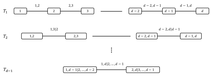
Figure 1: The structure of a general D-Vine on $d$ variables.

Wilson (2018) proposed considering Gaussian and $t$-copulas as candidate copulas, along with several Archi-medean copulas that are absolutely continuous with full support. These bivariate copulas were selected by soliciting estimates for the conditional quartiles of the $p_{v}$ and $Z_{v}$ variables. Across all candidate copula families considered, the best-fitting copula was parameterized to minimize least squares between the solicited and induced prior quantiles on the $Z_{v}$ variables. Wilson et al. (2021) asserted that these priors can be used as sampling distributions in Monte Carlo simulations or as prior distributions in Bayesian analyses.

1.3 Contributions

This paper provides general guidance for prior dependence specification in multivariate settings. These recommendations are topical given that recent advances in copula-based priors allow for the incorporation of unprecedented flexibility into the prior dependence structure. While this additional flexibility could give rise to priors that more accurately characterize real-life phenomena, practitioners may be subject to choice overload when deciding between the vast number of potential dependence structures. We argue that this additional flexibility is only appropriate for certain prior distributions. Our recommendations help practitioners discard prior dependence structures that are not suitable for posterior analysis – simplifying the prior specification process. These recommendations also clarify how the prior dependence structure can impact the posterior distribution. Our recommendations are illustrated using several models for which copula-based priors have been proposed. Flexible copula-based methods continue to be proposed as possible extensions in new settings (Perepolkin et al., 2023), so this paper’s commentary is broadly applicable. Unlike situations that require the specification of a community of prior distributions, we restrict our discussion to the case where a single prior is elicited.

The remainder of this article is structured as follows. In Section 2, we define general conditions under which the prior dependence structure is incompatible with that induced by the likelihood function and unable to be retained by the posterior distribution as data are observed. We formally prove this result and demonstrate that priors elicited using the methods proposed by Elfadaly and Garthwaite (2017) and Wilson (2018) are generally incompatible with standard likelihood functions. We clarify the settings for which this additional flexibility in the prior dependence structure is useful in Section 3. In Section 4, we prove several theoretical results about the impact of the prior dependence structure on the convergence of the posterior mode, which we contrast with previous work on copula-based priors (Michimae and Emura, 2022). We then conduct numerical studies to contextualize these theoretical results, which prompt general recommendations regarding choosing a prior dependence structure for posterior analysis. We provide concluding remarks and a discussion of extensions to this work in Section 5.

2 The Prior-Posterior Disconnect

2.1 Background

In this section, we examine situations where the prior dependence structure cannot carry over into the posterior distribution as data are collected. It is unrealistic to expect the prior dependence structure for $\boldsymbol{\theta}$ to be perfectly specified. However, it presents practical issues if we select a prior dependence structure that cannot be retained a posteriori and plan to use the posterior of $\boldsymbol{\theta}$ to draw conclusions about its dependence structure. This would lead us to draw different conclusions about the dependence structure given small and large samples generated from the same data generation process, giving rise to a disconnect between the prior and posterior. Such prior dependence structures also make it problematic to consider the posterior of a function of several parameters in $\boldsymbol{\theta}$.

We introduce the concept of chronic rejection (Libby and Pober, 2001; Vos et al., 2011) to frame this section’s main result. The term chronic rejection is often used to describe the process in which a transplanted organ is rejected by the recipient’s immune system over a long period of time. The recipient’s persistent immune response against the transplanted organ causes slow and gradual damage. This is in contrast to acute or hyperacute rejection that occurs shortly after the organ is transplanted. Chronic rejection is a more appropriate analogy for this work because we may require very large sample sizes for the vestiges of the prior dependence structure to disappear. Similar to finding a suitable organ donor, we argue that one should consider whether the prior dependence structure for $\boldsymbol{\theta}$ is compatible with that induced by the likelihood function. Such incompatibilities imply that the prior dependence structure cannot be retained a posteriori – and is hence chronically rejected. We emphasize that the term rejection as used in this paper does not imply the formal rejection of a statistical hypothesis test. In Section 2.2, we define broad conditions under which the posterior chronically rejects the prior dependence structure. We illustrate this phenomenon using simulation in Section 2.3.

2.2 Chronic Rejection of Prior Dependence in Posterior Distributions

Here, we define general conditions under which prior dependence structures are chronically rejected by the posterior. These sufficient conditions can be readily verified prior to observing data. When planning posterior analyses, practitioners can discard prior dependence structures that satisfy these conditions. This simplification reduces the number of potential dependence structures and hence streamlines the prior elicitation process.

We consider the limiting behaviour of the posterior distribution for $\boldsymbol{\theta}$. Because we consider this behaviour under various data generation processes, the data are random variables. Data from a random sample of size $n$ are represented by $\boldsymbol{Y}^{{}_{(n)}}$. Realizations of these samples are denoted by $\boldsymbol{y}^{{}_{(n)}}$. Much of the work on limiting posteriors (see e.g., (Ghosal et al., 1995), (Le Cam and Yang, 2000), (Gao et al., 2020), or (Schillings et al., 2020)) appeals to the Bernstein-von Mises theorem (van der Vaart, 1998). We let $m(\hskip 1.0pt\cdot\hskip 1.0pt|\hskip 1.0pt\boldsymbol{\theta})$ be the statistical model corresponding to the likelihood function in (1). When data $\boldsymbol{Y}^{{}_{(n)}}$ are generated independently and identically from $m(\hskip 1.0pt\cdot\hskip 1.0pt|\hskip 1.0pt\boldsymbol{\theta}_{0})$, the Bernstein-von Mises theorem dictates that the posterior for $\boldsymbol{\theta}$ converges to the $\mathcal{N}(\boldsymbol{\theta}_{0},\mathcal{I}(\boldsymbol{\theta}_{0})^{-1}/n)$ distribution in the limit of infinite data, where $\mathcal{I}(\cdot)$ is the Fisher information.

In addition to the independently and identically distributed assumption, there are three conditions that must be satisfied to invoke the Bernstein-von Mises theorem. The first two conditions involve the model $m(\hskip 1.0pt\cdot\hskip 1.0pt|\hskip 1.0pt\boldsymbol{\theta}_{0})$, and they are collectively weaker than the conditions for the asymptotic normality of the maximum likelihood estimator (MLE) (Lehmann and Casella, 1998). Condition 1 ensures the model $m(\hskip 1.0pt\cdot\hskip 1.0pt|\hskip 1.0pt\boldsymbol{\theta}_{0})$ is differentiable in quadratic mean with nonsingular $\mathcal{I}(\boldsymbol{\theta}_{0})$. Condition 2 requires that there exist a sequence of uniformly consistent tests for $H_{0}:\boldsymbol{\theta}=\boldsymbol{\theta}_{0}$ vs. $H_{1}:\lVert\boldsymbol{\theta}-\boldsymbol{\theta}_{0}\rVert_{2}\geq\varepsilon$ for every $\varepsilon>0$. Condition 3 concerns the prior distribution $p(\boldsymbol{\theta})$ used to analyze the observed data. This prior must be absolutely continuous in a neighbourhood of $\boldsymbol{\theta}_{0}$ with $p(\boldsymbol{\theta}_{0})>0$. We consider priors defined such that

$$p(\boldsymbol{\theta})=\prod_{j=1}^{d}f_{j}(\theta_{j})\times c(F_{1}(\theta_{1}),...,F_{d}(\theta_{d})),$$ (4)

where $c(u_{1},...,u_{d})$ is the copula density function for an absolutely continuous copula $C$ and $F_{j}(\theta_{j})$ and $f_{j}(\theta_{j})$ are respectively the marginal prior CDF and PDF for $\theta_{j}$, $j=1,...,d$. Our first result in Corollary 1 is a direct consequence of the Bernstien-von Mises theorem.

Corollary 1.

Let the model $m(\hskip 1.0pt\cdot\hskip 1.0pt|\hskip 1.0pt\boldsymbol{\theta}_{0})$ and prior $p(\boldsymbol{\theta})$ satisfy all conditions for the Bernstien-von Mises theorem. Let $\boldsymbol{Y}^{{}_{(n)}}$ be generated independently from $m(\hskip 1.0pt\cdot\hskip 1.0pt|\hskip 1.0pt\boldsymbol{\theta}_{0})$. The posterior dependence structure of $\boldsymbol{\theta}$ given observed $\boldsymbol{y}^{{}_{(n)}}$ converges to $C^{Ga}_{\boldsymbol{R}}(\cdot)$ corresponding to the covariance matrix $\mathcal{I}(\boldsymbol{\theta}_{0})^{-1}$ as $n\rightarrow\infty$.

By the Bernstein-von Mises theorem, the posterior of $\boldsymbol{\theta}$ is approximately multivariate normal with covariance matrix $\mathcal{I}(\boldsymbol{\theta}_{0})^{-1}/n$, so its dependence structure is reasonably characterized by a Gaussian copula with correlation matrix $\boldsymbol{R}$ corresponding to $\mathcal{I}(\boldsymbol{\theta}_{0})^{-1}$. We next extend this result to a more general setting where the observations in $\boldsymbol{Y}^{{}_{(n)}}$ are independently but not identically distributed. We now explore the limiting behaviour of the posterior when data are generated from the following prior predictive distribution of $\boldsymbol{Y}^{{}_{(n)}}$:

$$p(\boldsymbol{y}^{{}_{(n)}})=\int m(\boldsymbol{y}^{{}_{(n)}}|\hskip 1.0pt\boldsymbol{\theta})\hskip 1.0ptp_{D}(\boldsymbol{\theta})\hskip 1.0ptd\boldsymbol{\theta},$$ (5)

where $p_{D}(\boldsymbol{\theta})$ is a prior that characterizes the data generation process for $\boldsymbol{Y}^{{}_{(n)}}$. The prior in (5) may or may not be the same prior as $p(\boldsymbol{\theta})$ used to analyze the observed data in (4), which is often called the analysis prior. The Bernstein-von Mises theorem considers a special case of $p(\boldsymbol{y}^{{}_{(n)}})$ in which the prior $p_{D}(\boldsymbol{\theta})$ is degenerate. That is, $p_{D}(\boldsymbol{\theta}_{0})=1$ for a particular $\boldsymbol{\theta}_{0}\in\boldsymbol{\Theta}$, and 0 otherwise. In light of this, we emphasize that the prior that must satisfy condition 3 for the Bernstein-von Mises theorem is the analysis prior $p(\boldsymbol{\theta})$. Theorem 1 generalizes the result from Corollary 1 for nondegenerate priors $p_{D}(\boldsymbol{\theta})$ under certain conditions.

Theorem 1.

Let $\boldsymbol{\Theta}^{*}$ be the set of interior points in $\boldsymbol{\Theta}$. Suppose conditions 1, 2, and 3 for the Bernstein-von Mises theorem are satisfied for all possible $\boldsymbol{\theta}_{0}\in\boldsymbol{\Theta}^{*}$. Let the likelihood function $L(\boldsymbol{\theta};\hskip 1.0pt\boldsymbol{y})$ be globally log-concave for all $\boldsymbol{\theta}\in\boldsymbol{\Theta}^{*}$. Let data $\boldsymbol{Y}^{{}_{(n)}}$ be generated independently from $p(\boldsymbol{y}^{{}_{(n)}})$ in (5) where $p_{D}(\boldsymbol{\theta})=0$ for all $\boldsymbol{\theta}\notin\boldsymbol{\Theta}^{*}$. For sufficiently large $n$, the posterior dependence structure of $\boldsymbol{\theta}$ given observed $\boldsymbol{y}^{{}_{(n)}}$ is approximately characterized by $C^{Ga}_{\boldsymbol{R}}(\cdot)$ corresponding to the covariance matrix $\mathcal{I}(\tilde{\boldsymbol{\theta}})^{-1}$ for the posterior mode $\tilde{\boldsymbol{\theta}}=\text{arg\,max}_{\boldsymbol{\theta}}~{}p(\boldsymbol{\theta}\hskip 1.0pt|\hskip 1.0pt\boldsymbol{y}^{{}_{(n)}})$.

Proof of Theorem 1. The degeneracy of $p_{D}(\boldsymbol{\theta})$ is the only condition of the Bernstein-von Mises theorem that Theorem 1 relaxes: each observation can be generated independently from $m(\hskip 1.0pt\cdot\hskip 1.0pt|\hskip 1.0pt\boldsymbol{\theta})$ parameterized with a different value for $\boldsymbol{\theta}\sim p_{D}(\boldsymbol{\theta})$. The first sentence in Theorem 1 ensures that all other conditions for the Bernstein-von Mises theorem are satisfied for all interior points in $\boldsymbol{\Theta}$. Unlike in Corollary 1, we now require that the likelihood function $L(\boldsymbol{\theta};\hskip 1.0pt\boldsymbol{y}^{{}_{(n)}})$ be globally log-concave for all $\boldsymbol{\theta}_{0}\in\boldsymbol{\Theta}^{*}$, which ensures that the posterior of $\boldsymbol{\theta}$ is unimodal with mode $\tilde{\boldsymbol{\theta}}$ given large samples $\boldsymbol{y}^{{}_{(n)}}$. When the conditions for Theorem 1 are satisfied, $p(\boldsymbol{\theta}\hskip 1.0pt|\hskip 1.0pt\boldsymbol{y}^{{}_{(n)}})$ is approximated by the following multivariate normal distribution (Gelman et al., 2013) for sufficiently large $n$:

$$\mathcal{N}\left(\tilde{\boldsymbol{\theta}},\left[-\dfrac{\partial^{2}}{\partial\boldsymbol{\theta}^{2}}\text{log}(p(\boldsymbol{\theta}\hskip 1.0pt|\hskip 1.0pt\boldsymbol{y}^{{}_{(n)}}))\bigg{\lvert}_{\boldsymbol{\theta}=\tilde{\boldsymbol{\theta}}}\right]^{-1}\right).$$ (6)

The likelihood function’s impact on the posterior of $\boldsymbol{\theta}$ overwhelms that of the prior as the sample size $n$ increases. For sufficiently large $n$, we can therefore replace $p(\boldsymbol{\theta}\hskip 1.0pt|\hskip 1.0pt\boldsymbol{y}^{{}_{(n)}})$ in the variance term of (6) with $L(\boldsymbol{\theta};\hskip 1.0pt\boldsymbol{y}^{{}_{(n)}})$. It follows that the posterior of $\boldsymbol{\theta}$ given observed $\boldsymbol{y}^{{}_{(n)}}$ is approximately $\mathcal{N}(\tilde{\boldsymbol{\theta}},\mathcal{I}(\tilde{\boldsymbol{\theta}})^{-1}/n)$ for sufficiently large samples $\boldsymbol{y}^{{}_{(n)}}$. Thus, the posterior dependence structure is approximately characterized by the Gaussian copula corresponding to the covariance matrix $\mathcal{I}(\tilde{\boldsymbol{\theta}})^{-1}$.∎

Under the conditions in Theorem 1, the posterior copula for $\boldsymbol{\theta}$ is approximately Gaussian for large samples. However, we may not collect nearly enough data for this copula to be Gaussian in practice. Because it is unrealistic to expect the prior dependence structure of $\boldsymbol{\theta}$ to be perfectly specified, we consider a partial characterization of this prior (and posterior) dependence structure using D-vines in Corollary 2. Even if the copula in (4) is not specified using a D-vine, such a structure can be induced. D-vines are often specified via the set of Kendall’s $\tau$ (Kendall, 1938) values for each of the D-vine’s bivariate copulas (Kurowicka and Cooke, 2005). Kendall’s $\tau$ measures rank correlation in terms of how similar the orderings of bivariate data are when ranked by each quantity. We let $\{\tau^{p}_{e_{1},e_{2}|D_{\boldsymbol{e}}}\}_{\boldsymbol{e}\in E(\mathcal{V})}$ characterize the prior dependence structure on $\boldsymbol{\theta}$.

Corollary 2.

Suppose the conditions for Theorem 1 are satisfied. Let $\{\tau^{p}_{e_{1},e_{2}|D_{\boldsymbol{e}}}\}_{\boldsymbol{e}\in E(\mathcal{V})}$ describe prior dependence on $\boldsymbol{\theta}$. If no $\boldsymbol{\theta}\in\boldsymbol{\Theta}^{*}$ is such that $C^{Ga}_{\boldsymbol{R}}(\cdot)$ corresponding to the covariance matrix $\mathcal{I}(\boldsymbol{\theta})^{-1}$ induces a dependence structure $\{\tau(\boldsymbol{\theta})_{e_{1},e_{2}|D_{\boldsymbol{e}}}\}_{\boldsymbol{e}\in E(\mathcal{V})}$ such that $\tau(\boldsymbol{\theta})_{e_{1},e_{2}|D_{\boldsymbol{e}}}=\tau^{p}_{e_{1},e_{2}|D_{\boldsymbol{e}}}$ for all $\boldsymbol{e}\in E(\mathcal{V})$, the posterior of $\boldsymbol{\theta}$ cannot retain the magnitude and direction of prior dependence as data $\boldsymbol{Y}^{{}_{(n)}}$ are generated independently from $p(\boldsymbol{y}^{{}_{(n)}})$ in (5) where $p_{D}(\boldsymbol{\theta})=0$ for all $\boldsymbol{\theta}\notin\boldsymbol{\Theta}^{*}$.

Corollary 2 follows directly from Theorem 1. We suppose that there is no $\boldsymbol{\theta}\in\boldsymbol{\Theta}^{*}$ such that the Gaussian copula corresponding to the covariance matrix $\mathcal{I}(\boldsymbol{\theta})^{-1}$ induces a dependence structure characterized by $\{\tau^{p}_{e_{1},e_{2}|D_{\boldsymbol{e}}}\}_{\boldsymbol{e}\in E(\mathcal{V})}$. Thus, it is impossible for the Gaussian copula corresponding to the covariance matrix $\mathcal{I}(\tilde{\boldsymbol{\theta}})^{-1}$ to induce a dependence structure with that partial characterization for $\tilde{\boldsymbol{\theta}}\in\boldsymbol{\Theta}^{*}$. It follows that the magnitude and direction of the dependence structure for $p(\boldsymbol{\theta}\hskip 1.0pt|\hskip 1.0pt\boldsymbol{y}^{{}_{(n)}})$ cannot be characterized by $\{\tau^{p}_{e_{1},e_{2}|D_{\boldsymbol{e}}}\}_{\boldsymbol{e}\in E(\mathcal{V})}$ for sufficiently large $n$. We emphasize that considering dependence structures via Kendall’s tau on the D-vine structure of the copula does not fully specify the dependence structure. This allows for more flexibility in the choices for the copula families; it also facilitates the consideration of prior dependence for subvectors of $\boldsymbol{\theta}$, which is useful because it may require too much cognitive complexity to assess the full prior dependence structure. However, two bivariate copulas may have the same Kendall’s tau but different properties in terms of symmetry and tail dependence. We focus on the magnitude and direction of dependence to present generally applicable guidance for prior specification. Corollary 2 therefore provides a straightforward result that can be used to discard potential dependence structures for $\boldsymbol{\theta}$ that will be chronically rejected as data $\boldsymbol{y}^{{}_{(n)}}$ are observed.

We now illustrate how Corollary 2 can be applied in several scenarios. We first consider prior specification for $\boldsymbol{\theta}=(\mu,\sigma^{2})$ in the typical $\mathcal{N}(\mu,\sigma^{2})$ model. For this model, the inverse Fisher information matrix $\mathcal{I}(\boldsymbol{\theta})^{-1}$ is diagonal for all possible values of $\mu\in\mathbb{R}$ and $\sigma^{2}\in\mathbb{R}^{+}$. It follows by Corollary 2 that the joint posterior of $\mu$ and $\sigma^{2}$ cannot retain a prior dependence structure for which Kendall’s tau is not 0. Under the conditions for Theorem 1, any attempt to inject positive or negative dependence into this posterior will be unsuccessful in the limit of infinite data. We also consider the standard gamma model parameterized by $\boldsymbol{\theta}=(\alpha,\beta)$, where $\alpha$ and $\beta$ are respectively the shape and rate parameters. The correlation between $\alpha$ and $\beta$ dictated by the inverse Fisher information matrix is $1/\sqrt{\alpha\psi_{1}(\alpha)}$, where $\psi_{1}(\cdot)$ is the trigamma function. The correlation $1/\sqrt{\alpha\psi_{1}(\alpha)}$ is a positive and increasing function for all $\alpha>0$. When the conditions for Theorem 1 hold, the joint posterior of $\boldsymbol{\theta}$ will be unable to retain negative dependence structures between $\alpha$ and $\beta$. The last model considered in this subsection is the multinomial model. In Section SM1 of the supplementary materials, we show that the inverse Fisher information matrix for the multinomial model parameterized in terms of $\boldsymbol{\theta}=(Z_{1},Z_{2},...,Z_{w-1})$ from (2) is diagonal for all possible $(Z_{1},Z_{2},...,Z_{w-1})\in(0,1)^{w-1}$. When combined with the standard multinomial likelihood, the prior specification methods proposed by Elfadaly and Garthwaite (2017) and Wilson (2018) satisfy the conditions for Theorem 1. If $p(\boldsymbol{\theta})$ incorporates any positive or negative dependence between the parameters, this dependence structure will be rejected as multinomial data $\boldsymbol{y}^{{}_{(n)}}$ are observed – even when $p_{D}(\boldsymbol{\theta})$ from the prior predictive distribution in (5) is the same as the analysis prior $p(\boldsymbol{\theta})$!

2.3 Illustration with Copula-Based Priors for the Multinomial Model

We now illustrate that prior dependence structures specified using the methods proposed by Elfadaly and Garthwaite (2017) and Wilson (2018) are routinely rejected when combined with the standard multinomial likelihood as data are observed. We consider the multinomial model with $w=3$ categories, which is parameterized by conditional probabilities $\boldsymbol{\theta}=(Z_{1},Z_{2})$. We specify $p(\boldsymbol{\theta})$ as in (4) where the marginal prior for $Z_{1}$ is $\text{BETA}(20,40)$, the marginal prior for $Z_{2}$ is $\text{BETA}(30,30)$, and these marginal priors are joined using a Gaussian copula parameterized with Pearson’s $\rho=-0.9$. This prior distribution conveys that we expect the multinomial probabilities to be roughly equal for all three categories. This prior specification could be facilitated using either of the methods by Elfadaly and Garthwaite (2017) and Wilson (2018). We note that the prior copula gives rise to a value for Kendall’s tau of $2\text{sin}^{-1}(-0.9)/\pi=-0.713$.

For illustration, we generate $10^{5}$ observations from the prior predictive distribution in (5) defined with $m(\hskip 1.0pt\cdot\hskip 1.0pt|\hskip 1.0pt\boldsymbol{\theta})$ corresponding to the standard multinomial model and $p(\boldsymbol{\theta})$ as detailed in the previous paragraph. In Figure 2, we visualize the prior copula along with the posterior copula for $\boldsymbol{\theta}$ given $\boldsymbol{y}^{{}_{(n)}}$ corresponding to the first $n=10^{1},10^{2},10^{3}$, $10^{4}$, and $10^{5}$ observations from the generated sample. This figure shows that the posterior cannot retain the negative dependence structure present in the prior as data are observed from the prior predictive distribution. Even though the prior $p(\boldsymbol{\theta})$ accurately characterizes the data generation process for the multinomial data, the multinomial likelihood function cannot accommodate this dependence between $Z_{1}$ and $Z_{2}$. As the sample size increases, we observe that the impact of the likelihood function on the posterior overwhelms that of the prior. We may require a very large multinomial sample, but the prior dependence structure will eventually be rejected when the conditions for Theorem 1 hold.

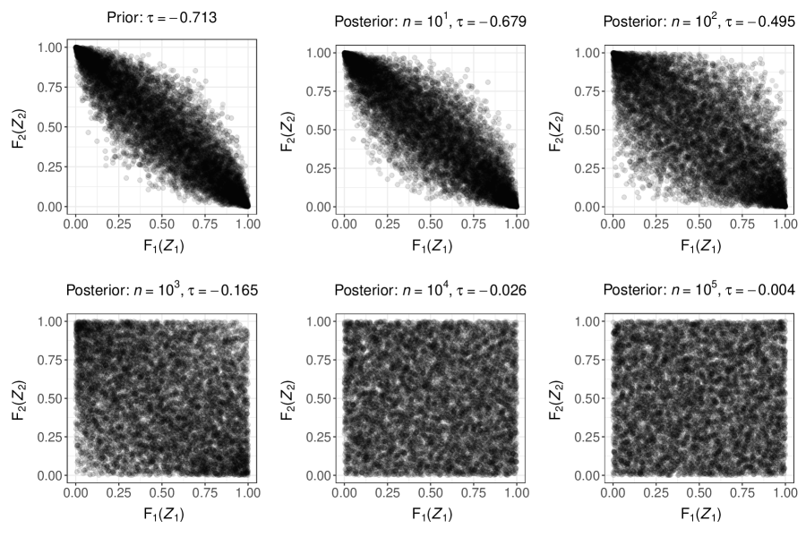
Figure 2: Rejection of negative prior dependence in the joint posterior of $Z_{1}$ and $Z_{2}$ at sample sizes $n=10^{1},10^{2},10^{3}$, $10^{4}$, and $10^{5}$.

The copula-based priors proposed by Elfadaly and Garthwaite (2017) and Wilson (2018) define valid posteriors for $\boldsymbol{\theta}$ when combined with the multinomial likelihood, but Figure 2 corroborates that we would draw vastly different conclusions about the posterior dependence structure of $\boldsymbol{\theta}$ for small and large samples. Elfadaly and Garthwaite (2017) provided R code to combine their priors with the multinomial likelihood function, and Wilson et al. (2021) stated that these priors could be used as prior distributions in Bayesian analyses. However, neither contribution clearly disclosed that these more flexible prior dependence structures cannot be retained as multinomial data are collected. Perhaps the posterior should be defined using a likelihood function for categorical data that allows for this dependence if these more flexible dependence structures are plausible a priori. This work does not consider how such modifications might allow for more flexible dependence structures to be retained a posteriori. Instead, we alert practitioners to situations where chronic rejection of prior dependence occurs. The adequacy stage of the prior elicitation framework proposed by Garthwaite et al. (2005) involves examining the prior’s fitness for purpose. Given a candidate prior dependence structure, Corollary 2 helps assess whether $p(\boldsymbol{\theta})$ is a suitable analysis prior. We note that prior distributions may be elicited to serve different purposes, and we elaborate on these situations in Section 3.

3 Design Priors

We clarify that the flexible dependence structures facilitated by copula-based priors are useful in certain situations. Not all prior distributions are elicited with the intent of defining a posterior. Prior distributions are regularly used for design purposes. For instance, priors might be used to summarize expert opinion to choose inputs for a decision model (Garthwaite et al., 2005). Design priors are also used in experimental settings to conduct sample size determination (De Santis, 2007; Berry et al., 2011; Gubbiotti and De Santis, 2011). In these settings, design priors are often informative and concentrated on $\boldsymbol{\theta}$ values that are relevant to the objective of the study. The prior $p_{D}(\boldsymbol{\theta})$ from (5) could be considered as a design prior in the context of this paper. The design prior is sometimes called the sampling prior, whereas the analysis prior $p(\theta)$ in (4) is sometimes named the fitting prior (Wang and Gelfand, 2002; Sahu and Smith, 2006).

Wilson (2018) illustrated the elicitation method with vine copulas using a multinomial model that characterized various states for the capacity of a complex engineering system. It is possible that the additional flexibility in the copula-based prior allows for subject matter expertise to be more accurately characterized. Perhaps this improved accuracy could give rise to better mitigation of safety implications associated with the engineering system. In that case, there may be value in taking the extra effort to specify a vine copula. If this more flexible prior were not combined with the multinomial likelihood function, there would be no concerns with such an approach. However, it is difficult for practitioners to make informed decisions about whether specifying a prior copula is worthwhile when it is not transparent that this additional effort could undermine the credibility of their posterior analysis. Copula-based prior elicitation procedures – such as those proposed by Elfadaly and Garthwaite (2017) and Wilson (2018) – are therefore useful in design settings, but conditions for their responsible use should be more clearly defined.

4 Impact of the Prior Copula on the Posterior

4.1 Convergence of the Posterior Mode

For an arbitrary model, it may be challenging to correctly specify the dependence structure a priori. As such, we consider how the choice of copula for the prior distribution impacts the posterior. We suppose that two potential priors for $\boldsymbol{\theta}$, denoted $p_{1}(\boldsymbol{\theta})$ and $p_{2}(\boldsymbol{\theta})$, are defined as in (4) using the same marginal distributions $F_{1},...,F_{d}$ but different copula density functions $c_{1}(\boldsymbol{u})$ and $c_{2}(\boldsymbol{u})$. We require that both copula density functions are absolutely continuous and twice differentiable with respect to $\boldsymbol{u}=(u_{1},...,u_{d})$. To ensure the domain of the parameter space is not inadvertently restricted, the priors should be chosen such that $p_{1}(\boldsymbol{\theta})>0$ and $p_{2}(\boldsymbol{\theta})>0$ for all $\boldsymbol{\theta}\in\boldsymbol{\Theta}$.

We define posteriors $p_{1}(\boldsymbol{\theta}\hskip 1.0pt|\hskip 1.0pt\boldsymbol{y}^{{}_{(n)}})$ and $p_{2}(\boldsymbol{\theta}\hskip 1.0pt|\hskip 1.0pt\boldsymbol{y}^{{}_{(n)}})$ by combining the likelihood $L(\boldsymbol{\theta};\hskip 1.0pt\boldsymbol{y}^{{}_{(n)}})$ for the model $m(\boldsymbol{y}^{{}_{(n)}}\hskip 1.0pt|\hskip 1.0pt\boldsymbol{\theta})$ with $p_{1}(\boldsymbol{\theta})$ and $p_{2}(\boldsymbol{\theta})$, respectively. We summarize each posterior via its posterior mode for $\boldsymbol{\theta}$, denoted by $\tilde{\boldsymbol{\theta}}^{{}_{(k)}}=\text{arg\,max}_{{\boldsymbol{\theta}}}~{}p_{k}(\boldsymbol{\theta}\hskip 1.0pt|\hskip 1.0pt\boldsymbol{y}^{{}_{(n)}})$ for $k=1,2$. In this section, we consider the convergence of the posterior mode to a fixed value $\boldsymbol{\theta}_{0}$. Unlike in Theorem 1, we exclusively consider degenerate priors $p_{D}(\boldsymbol{\theta})$ for the prior predictive distribution of $\boldsymbol{Y}^{{}_{(n)}}$ in (5). This restriction is necessary for the posterior of $\boldsymbol{\theta}$ to converge around the fixed value $\boldsymbol{\theta}_{0}$. This degenerate prior $p_{D}(\boldsymbol{\theta})$ is distinct from the analysis priors $p_{1}(\boldsymbol{\theta})$ and $p_{2}(\boldsymbol{\theta})$ used to define the relevant posteriors. For a given sample $\boldsymbol{y}^{{}_{(n)}}$, we compare the Euclidean distance between $\boldsymbol{\theta}_{0}$ and each posterior mode, denoted by $\mathcal{D}_{k}=\lVert\tilde{\boldsymbol{\theta}}^{{}_{(k)}}-\boldsymbol{\theta}_{0}\rVert_{2}$ for $k=1,2$. Theorem 2 indicates that we generally do not expect the choice of prior copula to impact whether the posterior mode is closer to $\boldsymbol{\theta}_{0}$ for large sample sizes $n$.

Theorem 2.

Let all conditions for the Bernstein-von Mises theorem be satisfied such that $\boldsymbol{Y}^{{}_{(n)}}$ is generated independently from $m(\hskip 1.0pt\cdot\hskip 1.0pt|\hskip 1.0pt\boldsymbol{\theta}_{0})$. Let priors $p_{1}(\boldsymbol{\theta})$ and $p_{2}(\boldsymbol{\theta})$ be defined as in (4) with the same marginals $F_{1},...,F_{d}$ but different copula density functions $c_{1}(\cdot)$ and $c_{2}(\cdot)$ that are absolutely continuous and twice differentiable. Suppose $p_{1}(\boldsymbol{\theta})>0$ and $p_{2}(\boldsymbol{\theta})>0$ for all $\boldsymbol{\theta}\in\boldsymbol{\Theta}$. Given observed $\boldsymbol{y}^{{}_{(n)}}$, define posteriors $p_{k}(\boldsymbol{\theta}\hskip 1.0pt|\hskip 1.0pt\boldsymbol{y}^{{}_{(n)}})\propto L(\boldsymbol{\theta};\hskip 1.0pt\boldsymbol{y}^{{}_{(n)}})\hskip 1.0ptp_{k}(\boldsymbol{\theta})$ with posterior mode $\tilde{\boldsymbol{\theta}}^{{}_{(k)}}$ for $k=1,2$. Let $\boldsymbol{u}_{0}=(F_{1}(\theta_{1,0}),...,F_{d}(\theta_{d,0}))$ and $\mathcal{D}_{k}=\lVert\tilde{\boldsymbol{\theta}}^{{}_{(k)}}-\boldsymbol{\theta}_{0}\rVert_{2}$ for $k=1,2$.

1. If $\nabla_{\boldsymbol{u}}\big{[}\emph{log}(c_{2}(\boldsymbol{u}))-\emph{log}(c_{1}(\boldsymbol{u}))\big{]}_{\boldsymbol{u}=\boldsymbol{u}_{0}}\neq\boldsymbol{0}$, then $\lim_{n\rightarrow\infty}Pr(\mathcal{D}_{2}\leq\mathcal{D}_{1})=0.5$.

2. If $\boldsymbol{u}_{0}$ is a local maximum of $\emph{log}(c_{2}(\boldsymbol{u}))-\emph{log}(c_{1}(\boldsymbol{u}))$, then $\lim_{n\rightarrow\infty}Pr(\mathcal{D}_{2}\leq\mathcal{D}_{1})=1$.

Theorem 2 explains that whether the choice of prior copula gives rise to faster convergence depends on the function $\text{log}(c_{2}(\boldsymbol{u}))-\text{log}(c_{1}(\boldsymbol{u}))$. While $c_{1}(\cdot)$ and $c_{2}(\cdot)$ are functions of $\boldsymbol{\theta}$ because $\boldsymbol{u}=(F_{1}(\theta_{1}),...,F_{d}(\theta_{d}))$, we consider the partial derivatives of the copula log-density functions with respect to $\boldsymbol{u}$ instead of $\boldsymbol{\theta}$. For $j=1,...,d$, it follows by the chain rule that

$$\begin{split}\frac{\partial}{\partial\theta_{j}}\bigg{[}\text{log}(c_{2}(\boldsymbol{u}))-\text{log}(c_{1}(\boldsymbol{u}))\bigg{]}=\\ f_{j}(\theta_{j})\frac{\partial}{\partial u_{j}}\bigg{[}\text{log}(c_{2}(\boldsymbol{u}))-\text{log}(c_{1}(\boldsymbol{u}))\bigg{]}.\end{split}$$ (7)

We can factor out the $f_{j}(\theta_{j})$ term because $p_{1}(\boldsymbol{\theta})$ and $p_{2}(\boldsymbol{\theta})$ are defined using the same marginals. The priors were also defined such that $p_{1}(\boldsymbol{\theta})>0$ and $p_{2}(\boldsymbol{\theta})>0$ for all $\boldsymbol{\theta}\in\boldsymbol{\Theta}$. Therefore, $f_{j}(\theta_{j})$ must be positive, and the partial derivative in (7) with respect to $\theta_{j}$ is 0 if and only if the partial derivative with respect to $u_{j}$ is 0. This correspondence ensures the results from Theorem 2 generalize over different specifications for the marginal distributions. We prove both parts of Theorem 2 below.

Proof of Theorem 2(a). The posterior mode $\boldsymbol{\theta}^{{}_{(k)}}$ minimizes $-\text{log}(p_{k}(\boldsymbol{\theta}\hskip 1.0pt|\hskip 1.0pt\boldsymbol{y}^{{}_{(n)}}))$ for $k=1,2$. We have that

$$\begin{split}&-\text{log}(p_{2}(\boldsymbol{\theta}\hskip 1.0pt|\hskip 1.0pt\boldsymbol{y}^{{}_{(n)}}))\\ &=-l(\boldsymbol{\theta};\hskip 1.0pt\boldsymbol{y}^{{}_{(n)}}))-\sum_{j=1}^{d}\text{log}(f_{j}(\theta_{j}))-\text{log}(c_{1}(\boldsymbol{u}))+\\ &~{}~{}~{}~{}~{}~{}(\text{log}(c_{1}(\boldsymbol{u}))-\text{log}(c_{2}(\boldsymbol{u}))),\end{split}$$ (8)

where $l(\boldsymbol{\theta};\hskip 1.0pt\boldsymbol{y}^{{}_{(n)}}))$ is the log-likelihood function. The first three terms in (8) are equal to $-\text{log}(p_{1}(\boldsymbol{\theta}\hskip 1.0pt|\hskip 1.0pt\boldsymbol{y}^{{}_{(n)}}))$. When $\boldsymbol{\theta}=\boldsymbol{\theta}^{{}_{(1)}}$, it follows that $-\nabla_{\boldsymbol{\theta}}\text{log}(p_{1}(\boldsymbol{\theta}\hskip 1.0pt|\hskip 1.0pt\boldsymbol{y}^{{}_{(n)}}))=0$ and $-\nabla_{\boldsymbol{\theta}}\text{log}(p_{2}(\boldsymbol{\theta}\hskip 1.0pt|\hskip 1.0pt\boldsymbol{y}^{{}_{(n)}}))=-\nabla_{\boldsymbol{\theta}}\big{[}\text{log}(c_{1}(\boldsymbol{u}))-\text{log}(c_{2}(\boldsymbol{u}))\big{]}$. For large sample sizes $n$, the conditions for Theorem 2 ensure that the log-posterior $-\text{log}(p_{2}(\boldsymbol{\theta}\hskip 1.0pt|\hskip 1.0pt\boldsymbol{y}^{{}_{(n)}}))$ converges to its quadratic approximation about $\boldsymbol{\theta}=\boldsymbol{\theta}_{0}$. We use $\boldsymbol{\theta}^{{}_{(1)}}$ as a starting point for the Newton–Raphson method (Nocedal and Wright, 2006) with $-\text{log}(p_{2}(\boldsymbol{\theta}\hskip 1.0pt|\hskip 1.0pt\boldsymbol{y}^{{}_{(n)}}))$ to find $\boldsymbol{\theta}^{{}_{(2)}}$. Because the quadratic approximation is appropriate for large samples, only one iteration of the Newton–Raphson method is required to approximate $\boldsymbol{\theta}^{{}_{(2)}}$. We let $\mathcal{J}(\cdot)$ be the observed information. It follows that

$$\boldsymbol{\theta}^{{}_{(2)}}\approx\boldsymbol{\theta}^{{}_{(1)}}-\mathcal{J}(\boldsymbol{\theta}^{{}_{(1)}})^{-1}\nabla_{\boldsymbol{\theta}=\boldsymbol{\theta}^{{}_{(1)}}}\big{[}\text{log}(c_{1}(\boldsymbol{u}))-\text{log}(c_{2}(\boldsymbol{u}))\big{]}.$$ (9)

The conditions for Theorem 2 also guarantee that the posterior mode $\boldsymbol{\theta}^{{}_{(1)}}$ is approximately equal to the approximately normal MLE $\hat{\boldsymbol{\theta}}^{{}_{(1)}}$ for large samples $\boldsymbol{y}^{{}_{(n)}}$. Because the MLE is consistent, $\mathcal{J}(\boldsymbol{\theta}^{{}_{(1)}})^{-1}\approx\mathcal{J}(\boldsymbol{\theta}_{0})^{-1}$ for sufficiently large samples. By (7), we have that $\nabla_{\boldsymbol{\theta}=\boldsymbol{\theta}_{0}}\big{[}\text{log}(c_{1}(\boldsymbol{u}))-\text{log}(c_{2}(\boldsymbol{u}))\big{]}\neq\boldsymbol{0}$, so $\text{log}(c_{1}(\boldsymbol{u}))-\text{log}(c_{2}(\boldsymbol{u}))$ can be approximated by a plane (with common gradient) in a neighbourhood of $\boldsymbol{\theta}_{0}$. It follows that $\mathcal{J}(\boldsymbol{\theta}^{{}_{(1)}})^{-1}\nabla_{\boldsymbol{\theta}=\boldsymbol{\theta}^{{}_{(1)}}}\big{[}\text{log}(c_{1}(\boldsymbol{u}))-\text{log}(c_{2}(\boldsymbol{u}))\big{]}$ will be roughly constant for all large samples $\boldsymbol{y}^{{}_{(n)}}$ generated from $m(\hskip 1.0pt\cdot\hskip 1.0pt|\hskip 1.0pt\boldsymbol{\theta}_{0})$. For an arbitrary large sample $\boldsymbol{y}^{{}_{(n)}}$, we have that $\boldsymbol{\theta}^{{}_{(2)}}\approx\boldsymbol{\theta}^{{}_{(1)}}+\boldsymbol{b}$ for some constant $\boldsymbol{b}$ that does not depend on $\boldsymbol{y}^{{}_{(n)}}$ by (9). Since the posterior concentrates around $\boldsymbol{\theta}_{0}$ as the sample size $n$ increases, this common perturbation $\boldsymbol{b}$ will decrease in magnitude. $\boldsymbol{\theta}^{{}_{(1)}}$ is approximately normally distributed about $\boldsymbol{\theta}_{0}$ for large samples, so these small perturbations will shift $\boldsymbol{\theta}^{{}_{(2)}}\approx\boldsymbol{\theta}^{{}_{(1)}}+\boldsymbol{b}$ closer to $\boldsymbol{\theta}_{0}$ with probability of roughly 0.5 due to the symmetry of the normal distribution. ∎

Proof of Theorem 2(b). The results from (8) and (9) hold true as in part (a). Because $\boldsymbol{u}_{0}$ is a local minimum of $\text{log}(c_{1}(\boldsymbol{u}))-\text{log}(c_{2}(\boldsymbol{u}))$, the local linear approximation of this function is not serviceable at $\boldsymbol{\theta}=\boldsymbol{\theta}_{0}$. However, this implies that $-\nabla_{\boldsymbol{\theta}=\boldsymbol{\theta}^{{}_{(1)}}}\big{[}\text{log}(c_{1}(\boldsymbol{u}))-\text{log}(c_{2}(\boldsymbol{u}))\big{]}$ should be directed toward $\boldsymbol{\theta}_{0}$ for large samples $\boldsymbol{y}^{{}_{(n)}}$ when the quadratic approximation to the log-posterior is appropriate and $\boldsymbol{\theta}^{{}_{(1)}}\approx\boldsymbol{\theta}_{0}$. We let the orthonormal basis $\mathcal{B}$ be composed of the eigenvectors of $\mathcal{J}(\boldsymbol{\theta}^{{}_{(1)}})^{-1}$. Since $\mathcal{J}(\boldsymbol{\theta}^{{}_{(1)}})^{-1}$ is a positive definite matrix, the angle between $-\nabla_{\boldsymbol{\theta}=\boldsymbol{\theta}^{{}_{(1)}}}\big{[}\text{log}(c_{1}(\boldsymbol{u}))-\text{log}(c_{2}(\boldsymbol{u}))\big{]}$ and $-\mathcal{J}(\boldsymbol{\theta}^{{}_{(1)}})^{-1}\nabla_{\boldsymbol{\theta}=\boldsymbol{\theta}^{{}_{(1)}}}\big{[}\text{log}(c_{1}(\boldsymbol{u}))-\text{log}(c_{2}(\boldsymbol{u}))\big{]}$ will be acute. With respect to $\mathcal{B}$, the perturbation from $\boldsymbol{\theta}^{{}_{(1)}}$ to $\boldsymbol{\theta}^{{}_{(2)}}$ induced by the Newton-Raphson method is then directed in the same orthant of $\boldsymbol{\Theta}\subseteq\mathbb{R}^{d}$ that contains $\boldsymbol{\theta}_{0}$. It follows that for large samples, $\boldsymbol{\theta}^{{}_{(2)}}$ cannot be further from $\boldsymbol{\theta}_{0}$ than $\boldsymbol{\theta}^{{}_{(1)}}$ due to a perturbation in the wrong direction. However, $\boldsymbol{\theta}^{{}_{(2)}}$ could still be further from $\boldsymbol{\theta}_{0}$ than $\boldsymbol{\theta}^{{}_{(1)}}$ if the magnitude of the perturbation is too large. We argue that this cannot occur for an arbitrary large sample $\boldsymbol{y}^{{}_{(n)}}$ because both $p_{1}(\boldsymbol{\theta}\hskip 1.0pt|\hskip 1.0pt\boldsymbol{y}^{{}_{(n)}}))$ and $p_{2}(\boldsymbol{\theta}\hskip 1.0pt|\hskip 1.0pt\boldsymbol{y}^{{}_{(n)}}))$ will concentrate around $\boldsymbol{\theta}_{0}$ and $\boldsymbol{\theta}_{0}$ maximizes $\text{log}(c_{2}(\boldsymbol{u}))-\text{log}(c_{1}(\boldsymbol{u}))$ in a neighbourhood of this fixed point. If this perturbation is too large for a given sample $\boldsymbol{y}^{{}_{(n)}}$, this behaviour cannot persist as $n\rightarrow\infty$. For large samples, these small perturbations by the Newton-Raphson method will therefore shift $\boldsymbol{\theta}^{{}_{(2)}}$ closer to $\boldsymbol{\theta}_{0}$ with probability approaching 1. ∎

We note that if $\boldsymbol{u}_{0}$ is a local minimum of $\text{log}(c_{2}(\boldsymbol{u}))-\text{log}(c_{1}(\boldsymbol{u}))$, then $\lim_{n\rightarrow\infty}Pr(\mathcal{D}_{2}\leq\mathcal{D}_{1})=0$. This follows directly from part (b) of Theorem 2 by switching the labels on $c_{1}(\cdot)$ and $c_{2}(\cdot)$. The case where $\boldsymbol{u}_{0}$ is a saddle point of $\text{log}(c_{2}(\boldsymbol{u}))-\text{log}(c_{1}(\boldsymbol{u}))$ is excluded from both parts (a) and (b). In that case, $Pr(\mathcal{D}_{2}\leq\mathcal{D}_{1})$ may converge to a constant that is not 0.5 or 1. We explore the results from Theorem 2 via simulation and explain their practical implications in Section 4.2.

4.2 Practical Implications

Here, we conduct simulations to consider Theorem 2 in practice. To do so, we consider an example adapted from Michimae and Emura (2022), who recently suggested that joint priors based on Archimedean copulas lead to more accurate and concentrated posterior distributions in the context of Bayesian ridge regression. These recommendations are inconsistent with the results of Theorem 2. The accuracy and concentration of the posterior of $\boldsymbol{\theta}$ were considered via the total mean absolute error between the posterior median and a fixed parameter value $\boldsymbol{\theta}_{0}$. Michimae and Emura’s (2022) numerical studies showed that the posterior was more concentrated around $\boldsymbol{\theta}_{0}$ when the marginal priors for the regression coefficients were joined using (Archimedean) Clayton and Gumbel copulas (Nelsen, 2006) instead of more standard Gaussian copulas. They considered a ridge regression model with three regression coefficients in the presence of multicollinearity, where the parameters of the relevant prior copulas were random variables specified using a hierarchical framework. The simplified example for our numerical study adapts aspects of their model for illustrative purposes.

Our simplified example considers the following linear regression model for the outcome $y_{i}$ and predictors $x_{i1}$ and $x_{i2}$:

$$y_{i}=\beta_{1}x_{i1}+\beta_{2}x_{i2}+\varepsilon_{i},$$

where $\varepsilon_{i}\sim\mathcal{N}(0,5)$ independently for $i=1,...,n$. The assumptions that the linear equation has an intercept of zero and the error terms have known variance reduce the dimensionality of the problem for illustration. That is, $\boldsymbol{\theta}=(\beta_{1},\beta_{2})$. We specify standard normal marginal priors for both $\beta_{1}$ and $\beta_{2}$.

We join these marginal priors with two prior copulas in this numerical study: $c_{1}(\boldsymbol{u})=1$ for $\boldsymbol{u}\in(0,1)^{2}$ corresponds to the independence copula and $c_{2}(\boldsymbol{u})$ corresponds to a two-dimensional $t$-copula with $\nu=4$ degrees of freedom and a diagonal correlation matrix $\boldsymbol{R}$. We select the first copula because it is often assumed that the regression coefficients are independent a priori in Bayesian regression models. The corresponding joint prior for $\beta_{1}$ and $\beta_{2}$ is therefore a standard bivariate normal distribution with diagonal $\boldsymbol{R}$. The choice for the second copula is motivated by $c_{2}(\boldsymbol{u})$ having a local maximum and saddle points to illustrate the results from Theorem 2. Figure 3 visualizes the logarithm of this copula density function. The selected $t$-copula does not accommodate strong negative or positive dependence between $\beta_{1}$ and $\beta_{2}$, but it reflects a greater likelihood of observing extreme values for both $\beta_{1}$ and $\beta_{2}$ relative to their marginal priors. For instance, this might occur if both marginal priors were misspecified.

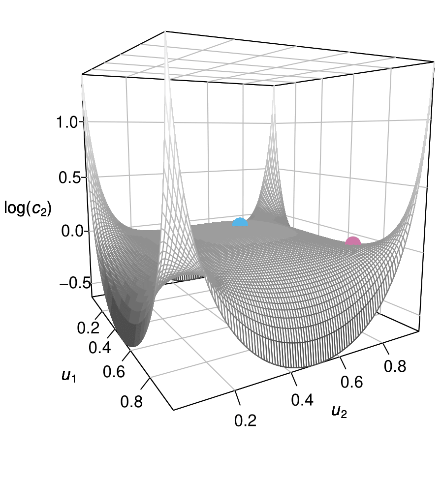
Figure 3: The logarithm of the $t$-copula density function with diagonal $\boldsymbol{R}$ and $\nu=4$. The local maximum at $\boldsymbol{u}=(0.5,0.5)$ and saddle point at $\boldsymbol{u}=(0.813,0.813)$ are given by the blue and pink points, respectively.

We consider six values for $\boldsymbol{\theta}_{0}$ to define the data generation process for $\boldsymbol{Y}^{{}_{(n)}}$. These six values are meant to illustrate the convergence of the posterior mode in a variety of settings. Because $\boldsymbol{u}_{0}=(F_{1}(\theta_{1,0},F_{2}(\theta_{2,0})))$, we can readily convert between $\boldsymbol{\theta}_{0}$ and $\boldsymbol{u}_{0}$ given the specified $\mathcal{N}(0,1)$ marginals. The marginal priors for $\beta_{1}$ and $\beta_{2}$ were chosen to be rather informative so that we observe a range of behaviour for the settings corresponding to part $(a)$ of Theorem 2.

For each $\boldsymbol{\theta}_{0}$ value, we generated 10000 samples of size $n$ for various sample sizes between 5 and $10^{5}$. Each observation was simulated independently as $y_{i}=\theta_{1,0}x_{i1}+\theta_{2,0}x_{i2}+\varepsilon_{i}$, where $(x_{i1},x_{i2})\sim\mathcal{N}(\boldsymbol{0},I_{2})$ and $\varepsilon_{i}\sim\mathcal{N}(0,5)$ for $i=1,...,n$. For each of these 10000 samples, we found both posterior modes $\tilde{\boldsymbol{\theta}}^{{}_{(1)}}$ and $\tilde{\boldsymbol{\theta}}^{{}_{(2)}}$. We then estimated $Pr(\mathcal{D}_{2}\leq\mathcal{D}_{1})$ as the proportion of samples for which $\tilde{\boldsymbol{\theta}}^{{}_{(2)}}$, corresponding to the $t$-copula, was closer to $\boldsymbol{\theta}_{0}$ than $\tilde{\boldsymbol{\theta}}^{{}_{(1)}}$. To consider the practical impact of Theorem 2, we also computed the mean absolute difference between $\mathcal{D}_{2}$ and $\mathcal{D}_{1}$ for each sample size $n$. Figure 4 visualizes these results for each of the six scenarios, which we now describe.

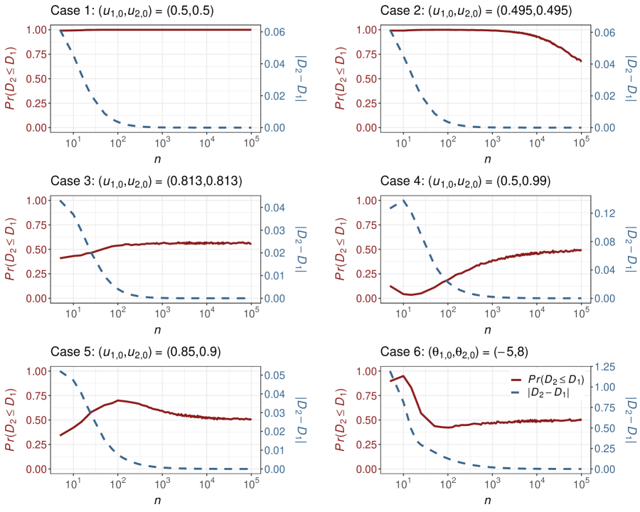
Figure 4: Estimated probability that $\tilde{\boldsymbol{\theta}}^{{}_{(2)}}$ is closer to $\boldsymbol{\theta}_{0}$ than $\tilde{\boldsymbol{\theta}}^{{}_{(1)}}$ (solid red) and mean absolute difference between $\mathcal{D}_{2}$ and $\mathcal{D}_{1}$ (dashed blue) as a function of $n$ on the logarithmic scale (base 10) for six $\boldsymbol{\theta}_{0}$ values.

We first consider case 1, where $\boldsymbol{u}_{0}$ = (0.5, 0.5). This point is a local maximum of $c_{2}(\boldsymbol{u})$ and therefore also a local maximum of $\text{log}(c_{2}(\boldsymbol{u}))-\text{log}(c_{1}(\boldsymbol{u}))=\text{log}(c_{2}(\boldsymbol{u}))$. As indicated by Theorem 2, the probability that $\tilde{\boldsymbol{\theta}}^{{}_{(2)}}$ is closer to $\boldsymbol{\theta}_{0}$ than $\tilde{\boldsymbol{\theta}}^{{}_{(1)}}$ approaches 1 as $n\rightarrow\infty$. Even though $\mathcal{D}_{2}$ is less than $\mathcal{D}_{1}$, their absolute difference is practically negligible for large sample sizes $n$. Case 2 considers a point $\boldsymbol{u}_{0}$ = (0.495, 0.495) that is extremely close to the local maximum. The plot for case 2 is similar to the previous one for small $n$, but the estimate for $Pr(\mathcal{D}_{2}\leq\mathcal{D}_{1})$ slowly decreases as $n\rightarrow\infty$. The estimated probability is still 0.673 for $n=10^{5}$. For $n=5\times 10^{6}$ (not pictured), we estimated $Pr(\mathcal{D}_{2}\leq\mathcal{D}_{1})$ to be 0.521. While $Pr(\mathcal{D}_{2}\leq\mathcal{D}_{1})$ approaches 0.5 in theory, it may not be 0.5 in practice if the sample size must be prohibitively large for the asymptotic result to hold. Case 3 examines a saddle point at $\boldsymbol{u}_{0}$ = ($\tilde{F}(1;4)$, $\tilde{F}(1;4)$), where $\tilde{F}(\cdot;4)$ is the CDF of the Student’s $t$-distribution with $\nu=4$ and $\tilde{F}(1;4)\approx 0.813$. This setting is noteworthy because $Pr(\mathcal{D}_{2}\leq\mathcal{D}_{1})$ does not approach 0.5 or 1. The probability for this scenario instead approaches 0.563, and we confirmed this limiting probability using samples of size $n=5\times 10^{6}$.

Case 4 considers a point $\boldsymbol{u}_{0}$ = (0.5, 0.99) where the independence copula performs better for smaller sample sizes in that the estimated probability approaches 0.5 from below. We note that $c_{2}(\boldsymbol{u}_{0})=0.533<1=c_{1}(\boldsymbol{u}_{0})$, which occurs because this bivariate $t$-copula deems scenarios where only one of $\beta_{1}$ or $\beta_{2}$ is extreme relative to their marginal priors as more rare than the independence copula. If $c_{2}(\boldsymbol{u}_{0})$ is less (greater) than $c_{1}(\boldsymbol{u}_{0})$, $Pr(\mathcal{D}_{2}\leq\mathcal{D}_{1})$ often approaches 0.5 from below (above). However, this behaviour is not guaranteed. Case 5 examines a point $\boldsymbol{u}_{0}$ = (0.85, 0.9) at which the estimated probability approaches 0.5 from above. Here, $c_{2}(\boldsymbol{u}_{0})=1.047>1$, but the estimate for $Pr(\mathcal{D}_{2}\leq\mathcal{D}_{1})$ is less than 0.5 for sample sizes less than $n=20$. Lastly, case 6 is defined in terms of its value for $\boldsymbol{\theta}_{0}=(\beta_{1,0},\beta_{2,0})=(-5,8)$ because the corresponding $\boldsymbol{u}_{0}$ value of ($2.87\times 10^{-7}$, $1-6.22\times 10^{-16}$) is quite extreme. For this setting, $c_{2}(\boldsymbol{u}_{0})=5054.68>>1$, and $\mathcal{D}_{2}$ is roughly 0.8 smaller than $\mathcal{D}_{1}$ on average for $n=10$. Yet, the estimated probability approaches 0.5 from below for large sample sizes. This likely occurs because $c_{2}(\boldsymbol{u})$ is volatile near $\boldsymbol{u}_{0}$.

We now contrast our conclusions from this numerical study with Michimae and Emura’s (2022) recommendations. First, the Clayton and Gumbel copulas used by Michimae and Emura (2022) only accommodate positive prior dependence between $\beta_{1}$ and $\beta_{2}$. If the covariates $x_{1}$ and $x_{2}$ are positively correlated, then the off-diagonal components in the inverse Fisher information matrix $\mathcal{I}(\tilde{\boldsymbol{\theta}})^{-1}$ evaluated at the posterior mode $\tilde{\boldsymbol{\theta}}$ will be negative for sufficiently large $n$. In this case, $\beta_{1}$ and $\beta_{2}$ will be unable to retain a postive dependence structure a posteriori. However, this does not constitute chronic rejection as defined in Section 2 because it is possible for $\beta_{1}$ and $\beta_{2}$ to retain their positive dependence a posteriori if $x_{1}$ and $x_{2}$ are negatively correlated. This example illustrates that the conditions for Theorem 1 are sufficient in that the prior dependence structure cannot be retained as data are observed when these conditions are satisfied. However, it is not guaranteed that the prior dependence structure will be retained when the conditions for Theorem 1 are not satisfied.

Our simulations demonstrate the value in considering the copula density functions $c_{1}(\boldsymbol{u})$ and $c_{2}(\boldsymbol{u})$ when choosing between two prior dependence structures. In particular, we may want to consider the local optima for the copula densities. This numerical study also suggests that copulas have limited ability to reliably prompt more accurate and concentrated posterior distributions around a fixed parameter value $\boldsymbol{\theta}_{0}$. The true value of $\boldsymbol{u}_{0}$ is unknown in practice. And even if $\boldsymbol{u}_{0}$ is such that $c_{2}(\boldsymbol{u}_{0})>c_{1}(\boldsymbol{u}_{0})$, it does not guarantee that $\tilde{\boldsymbol{\theta}}^{{}_{(2)}}$ will be closer to $\boldsymbol{\theta}_{0}$ than $\tilde{\boldsymbol{\theta}}^{{}_{(1)}}$ – for small or large sample sizes.

Michimae and Emura’s (2022) numerical studies considered several levels of multicollinearity between the regression covariates for a single $\boldsymbol{\theta}_{0}$ value. They also considered relatively small sample sizes ranging from $n=20$ to 200. Our numerical results suggest that it is pertinent to consider a variety of $\boldsymbol{\theta}_{0}$ values and sample sizes $n$ before making general statements about the impact of the prior copula on the posterior distribution. We acknowledge that Michimae and Emura (2022) considered a more complicated model, which leveraged a hierarchical framework to specify the prior copula. Although not the focus of this article, Monte Carlo simulation could likely be used to explore the local optima of such prior copula density functions and extend the results from Theorem 2 to a hierarchical framework. This extension is one of several possible generalizations that could be made to how the analysis prior in (4) is defined.

5 Discussion

In this paper, we emphasized the importance of considering whether prior dependence structures can be retained a posteriori when assessing the adequacy of multivariate prior distributions. We proved a theorem and resulting corollary that help discard potential prior dependence structures for a parameter $\boldsymbol{\theta}$ that will be routinely or chronically rejected as data are observed in general settings. Discarding such dependence structures simplifies the prior specification process. This corollary examined whether the prior dependence structure for $\boldsymbol{\theta}$ is compatible with that induced by the likelihood function. With this corollary, we critiqued past recommendations that suggested flexible copula-based priors were suitable as analysis priors. We argued that these priors are better suited for design purposes. This paper emphasized copula-based priors, but the notion of chronic rejection is still applicable to multivariate prior distributions that are not explicitly defined using copulas, such as multivariate normal priors. Because correctly specifying the dependence structure a priori for an arbitrary model may be difficult, we examined how the choice of prior copula impacts the posterior distribution. We proved several results regarding how this choice of copula impacts the convergence of the posterior mode to a fixed parameter value $\boldsymbol{\theta}_{0}$. While examining the local optima of candidate copula density functions is valuable, our numerical studies showed that prior copulas should not be selected to improve the posterior’s ability to recover $\boldsymbol{\theta}_{0}$.

Future work could extend the results from this paper to hierarchical settings, in which the hyperparameters of the prior copula are themselves random variables. Moreover, copula-based prior specification could also be applied in more complex designs. For example, much of the existing literature on prior elicitation focuses on the single model case. However, many studies seek to compare data from two groups, where the data from group $k$ is generated from the model $m_{k}(\hskip 1.0pt\cdot\hskip 1.0pt|\hskip 1.0pt\boldsymbol{\theta}_{k})$ for $k=1,2$. In the absence of information about one of the two groups, prior elicitation is an arduous task. When less is known about group 2, copulas might be used in conjunction with the prior information about group 1 to specify a joint prior for $\boldsymbol{\theta}_{1}$ and $\boldsymbol{\theta}_{2}$. Such methods could meaningfully facilitate design prior specification. Our results from this paper could be extended to provide guidance on whether these prior distributions would also be suitable analysis priors.

Supplementary Material

Section SM1 of the supplementary materials proves that the Fisher information for the conditional parameterization of the multinomial model is diagonal. The code for the numerical studies is provided on Github: https://github.com/lmhagar/PosteriorRamifications

Funding Acknowledgement

This work was supported by the Natural Sciences and Engineering Research Council of Canada (NSERC) by way of a PGS D scholarship as well as Grant RGPIN-2019-04212.

References

- Bedford and Cooke (2002) Bedford, T. and R. M. Cooke (2002). Vines–a new graphical model for dependent random variables. The Annals of Statistics 30(4), 1031 – 1068.
- Berry et al. (2011) Berry, S. M., B. P. Carlin, J. J. Lee, and P. Muller (2011). Bayesian adaptive methods for clinical trials. CRC press.
- Carlin and Louis (2000) Carlin, B. P. and T. A. Louis (2000). Bayes and empirical Bayes methods for data analysis (2 ed.). Springer.
- Casella (1985) Casella, G. (1985). An introduction to empirical Bayes data analysis. The American Statistician 39(2), 83–87.
- Casement and Kahle (2018) Casement, C. J. and D. J. Kahle (2018). Graphical prior elicitation in univariate models. Communications in Statistics-Simulation and Computation 47(10), 2906–2924.
- Casement and Kahle (2023) Casement, C. J. and D. J. Kahle (2023). The phoropter method: a stochastic graphical procedure for prior elicitation in univariate data models. Journal of the Korean Statistical Society 52(1), 60–82.
- Chaloner (1996) Chaloner, K. (1996). Elicitation of prior distributions. In Bayesian biostatistics, pp. 141–156. Marcel Dekker, New York.
- Chaloner et al. (1993) Chaloner, K., T. Church, T. A. Louis, and J. P. Matts (1993). Graphical elicitation of a prior distribution for a clinical trial. Journal of the Royal Statistical Society: Series D (The Statistician) 42(4), 341–353.
- Clemen and Reilly (1999) Clemen, R. T. and T. Reilly (1999). Correlations and copulas for decision and risk analysis. Management Science 45(2), 208–224.
- Connor and Mosimann (1969) Connor, R. J. and J. E. Mosimann (1969). Concepts of independence for proportions with a generalization of the Dirichlet distribution. Journal of the American Statistical Association 64(325), 194–206.
- Crispino and Antoniano-Villalobos (2023) Crispino, M. and I. Antoniano-Villalobos (2023). Informative priors for the consensus ranking in the bayesian mallows model. Bayesian Analysis 18(2), 391–414.
- De Santis (2007) De Santis, F. (2007). Using historical data for Bayesian sample size determination. Journal of the Royal Statistical Society: Series A (Statistics in Society) 170(1), 95–113.
- Demarta and McNeil (2005) Demarta, S. and A. J. McNeil (2005). The t copula and related copulas. International statistical review 73(1), 111–129.