First measurement of the Weyl potential evolution from the Year 3 Dark Energy Survey data: Localising the $\sigma_{8}$ tension

Abstract

We present the first measurement of the Weyl potential at four redshifts bins using data from the first three years of observations of the Dark Energy Survey (DES). The Weyl potential, which is the sum of the spatial and temporal distortions of the Universe’s geometry, provides a direct way of testing the theory of gravity and the validity of the $\Lambda$CDM model. We find that the measured Weyl potential is 2.3$\sigma$, respectively 3.1$\sigma$, below the $\Lambda$CDM predictions in the two lowest redshift bins. We show that these low values of the Weyl potential are at the origin of the $\sigma_{8}$ tension between Cosmic Microwave Background (CMB) measurements and weak lensing measurements. Interestingly, we find that the tension remains if no information from the CMB is used. DES data on their own prefer a high value of the primordial fluctuations, followed by a slow evolution of the Weyl potential. A remarkable feature of our method is that the measurements of the Weyl potential are model-independent and can therefore be confronted with any theory of gravity, allowing efficient tests of models beyond General Relativity.

I Introduction

Since the observation of the accelerated expansion of the Universe in 1998 SupernovaSearchTeam:1998fmf ; SupernovaCosmologyProject:1998vns , extensive studies have been performed to understand if this acceleration is due to a cosmological constant, a dynamical dark energy, or a modification of the theory of gravity. In theories beyond $\Lambda$CDM, not only the background evolution of the Universe can be modified, but also the formation of structure. A powerful way of testing these theories is therefore to confront them with measurements from large-scale structure surveys.

The landscape of theories beyond $\Lambda$CDM is vast, and testing all models one by one has become infeasible. As a consequence, two approaches have been developed over the years to efficiently probe deviations from a cosmological constant. The first one consists in testing classes of theories, e.g. Horndeski theories Horndeski1974 that encompass all scalar-tensor theories with second-order equations of motion. The advantage of such an approach is that the functions constrained by the data are directly linked to fundamental ingredients in the theories. However, the degeneracies between the free functions are large, and current data are not stringent enough to constrain them all well, see e.g. Noller:2018wyv .

The second approach is more phenomenological and consists in parameterising deviations from General Relativity (GR) directly at the level of Einstein’s equations by introducing two new functions, often called $\mu$ and $\eta$, see e.g. Koyama:2015vza . The function $\mu$ encodes changes in Poisson’s equation, while $\eta$ describes the difference between the time distortion and the spatial distortion of the metric, the so-called anisotropic stress. This approach has been successfully used with current data, e.g. combining gravitational lensing measurements from the Dark Energy Survey (DES) and galaxy clustering measurements from BOSS and eBOSS DES:2022ygi . Even though powerful, this approach suffers from one important complication: the constraints on $\mu$ and $\eta$ at a given redshift $z$ depend on the evolution of the functions at all redshifts above $z$. This means that either one needs to assume a given time evolution for these functions, as done in DES:2022ygi , in which case only the values of $\mu$ and $\eta$ at $z=0$ are constrained and the time evolution is fixed. Or one needs sophisticated techniques to constrain and reconstruct the time evolution of $\mu$ and $\eta$ from a set of chosen redshift nodes, as done for example in Bonvin:2022tii . In this second case, it is necessary to have measurements over a wide range of redshift to obtain relevant constraints, and any degradation of the data in a given redshift bin will impact the constraints in the other bins. Another limitation of this framework is that the constraints on $\mu$ and $\Sigma$ rely on the validity of Euler’s equation for dark matter. Without this additional assumption, $\mu$ cannot be constrained from redshift-space distortions (RSD), since it is fully degenerated with the parameters encoding changes in Euler’s equation SvevaNastassiaCamille ; Bonvin:2022tii . As a consequence, $\Sigma$ can also not be constrained if Euler’s equation is not valid.

In this paper, we propose an alternative approach, which is fully detached from any theoretical model. We ask ourselves: what are the quantities that we can directly measure from data, in a fully model-independent way? This approach is actually not new and it has been extensively used in the past for RSD. Combining the multipoles of the RSD correlation function (or power spectrum) provides direct measurements of the galaxy peculiar velocities in the redshift bins of the surveys. The evolution of the velocity is encoded in the so-called growth rate function, $f$, which is measured in combination with $\sigma_{8}$ (the amplitude of density perturbations in spheres of 8 Mpc/$h$) Song:2008qt ; Blake_2011 ; eBOSS:2020yzd . Such measurements are very powerful, since $f\sigma_{8}$ can then be compared with the prediction from GR to see if this theory is consistent or not. Moreover, it can be compared with predictions from any other theory of gravity, to put constraints on their parameters, see e.g. eBOSS:2020yzd .

To the best of our knowledge, this approach, which is standard in RSD analyses, has never been used for gravitational lensing analyses with real observations before. The goal of this paper is to do precisely that, using DES measurements of galaxy-galaxy lensing and galaxy clustering. More precisely, we use the formalism developed in Tutusaus:2022cab to measure the evolution of the Weyl potential $\Psi_{W}=(\Phi+\Psi)/2$ in four redshift bins, which correspond to the tomographic bins for the DES lenses. This provides the first direct and model-independent measurement of the evolution of the perturbed geometry of our Universe. We define a new function, $\hat{J}$, that we call the Weyl evolution, to encode the evolution of the Weyl potential. The measurement of $\hat{J}$ from DES data is fully complementary to the growth rate measurement. Modified theories of gravity can indeed change the way structures evolve, the way the geometry evolves, or both. As for the measurement of $f\sigma_{8}$, the Weyl evolution $\hat{J}$ is measured redshift bin per redshift bin, without assuming any time evolution.

We find that $\hat{J}$ can be measured with a precision of $4-9\%$ when $3\sigma$ priors from Planck are used to constrain early time cosmological parameters. These constraints mildly degrade to $5-11\%$ when only DES data are used. Imposing a more stringent scale cut on the angular correlation functions further degrades the constraints by a factor of 2. In the baseline analysis (i.e. with Planck priors and standard scale cuts), we find that the measurements of the Weyl evolution are 2.7$\sigma$, respectively 3.1$\sigma$, below the predictions from $\Lambda$CDM in the first and second redshift bins of DES. Assuming that $\Lambda$CDM is valid, these measurements can be used to infer the value of $\sigma_{8}$ today. Using priors from Planck we recover the well-known tension between CMB and weak lensing, which we find to be 2.5$\sigma$. More surprisingly, we find that the tension between the high redshift clustering amplitude and the low redshift clustering amplitude remains when no information from Planck is used.

Finally, we compare our measurements of $\hat{J}$ with various models of modified gravity. The flexibility of our method allows us to compare different time evolutions of the modified gravity parameters. While the constraining power of current data is too small to distinguish between various time evolutions, the coming generation of surveys like Euclid and LSST is expected to provide more stringent measurements of $\hat{J}$ over a wider redshift range, potentially allowing to reconstruct the time evolution using our method.

II The lensing angular power spectra as function of the Weyl evolution

The formalism to relate gravitational lensing observables to the Weyl evolution $\hat{J}$ has been derived in Tutusaus:2022cab . Here we summarise the main results.

We work with the linearly perturbed flat Friedmann-Lemaître-Robertson-Walker (FLRW) metric in the conformal Newtonian gauge, with the line element given by

$$\mathrm{d}s^{2}=a^{2}(\tau)\Big{[}-(1+2\Psi)\mathrm{d}\tau+(1+2\Phi)\mathrm{d}\mathbf{x}^{2}\Big{]}\,,$$ (1)

where $\tau$ denotes conformal time, $a$ is the scale factor, and $\Psi$ and $\Phi$ are the two metric potentials. Gravitational lensing is directly sensitive to the Weyl potential $\Psi_{W}\equiv(\Phi+\Psi)/2$. We define the Weyl transfer function $T_{\Psi_{W}}$, which relates the value of $\Psi_{W}(z,\mathbf{k})$ in Fourier space and at redshift $z$ to the primordial potential at the end of inflation $\Psi_{\rm in}(\mathbf{k})$. In GR, one can easily show that for wavelengths that are inside the horizon, the Weyl transfer function simply evolves proportionally to $D_{1}(z)\Omega_{\rm m}(z)$. Here $D_{1}$ is the growth function (governing the evolution of matter density perturbations) and $\Omega_{\rm m}(z)$ is the matter density parameter at redshift $z$. Hence, in GR, measuring the evolution of density perturbations or measuring the evolution of the Weyl potential provides exactly the same information. In modified theories of gravity the situation is different: Einstein’s equations are modified, generically leading to a different evolution of the Weyl potential. To capture this, we introduce a new function, $J$, encoding this evolution. More precisely, we write the transfer function of the Weyl potential as (see Tutusaus:2022cab for more detail )

$$T_{\Psi_{W}}(k,z)= \frac{\mathcal{H}^{2}(z)J(k,z)}{\mathcal{H}^{2}(z_{*})D_{1}(z_{*})}\frac{\sqrt{B(k,z)}}{\sqrt{B(k,z_{*})}}T_{\Psi_{W}}(k,z_{*})\,,$$ (2)

where $z_{*}$ is a redshift well in the matter era (before the acceleration of the Universe started), $\mathcal{H}$ is the Hubble parameter in conformal time, and $B(k,z)$ is a boost factor, encoding the non-linear evolution of matter density perturbations at small scales. We assume that at $z_{*}$ a cold dark matter (CDM) Universe, governed by GR, is recovered. This assumption automatically excludes early dark energy models, where deviations from a CDM Universe take place already at high redshift. The motivation behind this assumption is that, at early times, CMB measurements are highly compatible with a CDM Universe Planck:2018vyg . Theories of modified gravity therefore usually aim at recovering GR at high redshift, while leading to a phase of accelerated expansion at low redshift. In our framework, any deviation in the Weyl potential evolution during the phase of accelerated expansion is encoded in the free function $J$. By measuring this free function as a function of redshift, we will be able to reconstruct the Weyl evolution and assess its compatibility with GR predictions, or with the predictions of any theory of gravity we may want to test. Note that the function $J$ has the same information content as the function $L$ defined in Amendola:2012ky ; Amendola:2013qna , which identified for the first time the quantities that can be measured in a model-independent way from large-scale structure surveys.

In full generality, $J$ is a function of redshift and wavenumber $k$. In GR, the evolution is almost scale-independent, except from a small scale-dependence due to massive neutrinos. In our analysis we fix the sum of neutrino masses to 0.06 eV, leading to a scale-dependence in the growth of structure (and therefore in $J$) which is negligible Euclid:2019clj . In models of gravity beyond GR, $J$ can in principle depend on scales. However, in many models of modified gravity, it turns out that the evolution is scale-independent for sub-horizon modes, where the quasi-static approximation is valid Gleyzes:2015rua ; Raveri:2021dbu . In our analysis, we therefore drop the scale-dependence in $J$ (as is also usually done for measurements of the growth rate in RSD analyses Song:2008qt ; Blake_2011 ; eBOSS:2020yzd ). This simplifies the analysis, but it is not a fundamental limitation of the method, which can be extended to a scale-dependent $J$.

As observable we consider the galaxy-galaxy lensing angular power spectrum, i.e. the cross-correlation of cosmic shear of background galaxies with clustering of foreground lenses. As shown in Tutusaus:2022cab , the galaxy-galaxy lensing angular power spectrum can be written in the following way (using the Limber approximation):

$$C_{\ell}^{\Delta\kappa}(z_{i},z_{j})= \frac{3}{2}\int\text{d}z\,n_{i}(z)\mathcal{H}^{2}(z)\hat{b}_{i}(z)\hat{J}(z)B\left(k_{\ell},\chi\right)\frac{P_{\delta\delta}^{\rm lin}\left(k_{\ell},z_{*}\right)}{\sigma_{8}^{2}(z_{*})}\int\text{d}z^{\prime}n_{j}(z^{\prime})\frac{\chi^{\prime}(z^{\prime})-\chi(z)}{\chi(z)\chi^{\prime}(z^{\prime})}\,,$$ (3)

where $n_{i}$ and $n_{j}$ denote the galaxy distribution function of the lenses and sources, respectively, and $k_{\ell}\equiv(\ell+1/2)/\chi$, with $\chi$ the comoving distance. $P_{\delta\delta}^{\rm lin}$ is the linear matter power spectrum, evaluated here at redshift $z_{*}$. We see that the galaxy-galaxy lensing angular power spectrum depends on: 1) the density fluctuations at $z_{*}$ where GR is recovered; 2) the evolution of background quantities, $\mathcal{H}(z)$ and $\chi(z)$, which we assume here to be as in $\Lambda$CDM ; and 3) the functions $\hat{J}$ and $\hat{b}_{i}$ defined as

$$\hat{J}(z) \equiv\frac{J(z)\sigma_{8}(z)}{D_{1}(z)}=\frac{J(z)\sigma_{8}(z_{*})}{D_{1}(z_{*})}\,,$$ (4)

$$\hat{b}_{i}(z) \equiv b_{i}(z)\sigma_{8}(z)\,,$$ (5)

where $b_{i}$ is the linear galaxy bias in the tomographic redshift bin $i$. The second equality in Eq. (4) follows from the fact that $\sigma_{8}(z)$ is directly proportional to $D_{1}(z)$. As a consequence $\hat{J}$ and $J$ contain the same information about modified gravity, since they are related by the ratio $\sigma_{8}(z_{*})/D_{1}(z_{*})$ which does not depend on the modifications of gravity (since we assume that at $z_{*}$ GR is recovered).

Since $\hat{b}_{i}(z)$ and $\hat{J}(z)$ vary slowly with redshift, we can take them out of the integral in Eq. (3) and evaluate them at the mean redshift of the bin $z_{i}$. We see therefore, that by measuring the galaxy-galaxy lensing angular power spectrum for lenses at redshift $z_{i}$, we can directly measure the functions $\hat{J}$ and $\hat{b}_{i}$ at that redshift, in a fully model-independent way, i.e. without assuming any theory of gravity, nor specifying a redshift evolution for $\hat{J}$. The fact that galaxy-galaxy lensing depends on $\hat{J}$ at the redshift of the lenses follows from the fact that, in the Limber approximation, the signal is fully due to correlations between the Weyl potential and the galaxy density at the position of the lenses. All the other correlations along the photon’s trajectory are negligible. The situation for the shear angular power spectrum is different, since it depends on the integral of $\hat{J}$ from the sources to the observer. For this reason we do not consider it in our analysis. Note however that this could be done by introducing a function $\hat{J}$ which is piece-wise constant in some chosen redshift bins, with smooth interpolation between them.

Equation (3) shows that there is a degeneracy between $\hat{J}$ and $\hat{b}_{i}$, but this degeneracy can be easily broken by adding the clustering angular power spectrum which only depends on $\hat{b}_{i}$. Following DES:2021bpo , we use the Limber approximation to compute the galaxy clustering spectrum at large $\ell$

$$C_{\ell}^{\Delta\Delta}(z_{i},z_{j})= \int\text{d}z\,n_{i}(z)n_{j}(z)\frac{\mathcal{H}(z)(1+z)}{\chi^{2}(z)}\hat{b}_{i}(z)\hat{b}_{j}(z)B\left(k_{\ell},\chi\right)\frac{P_{\delta\delta}^{\rm lin}\left(k_{\ell},z_{*}\right)}{\sigma_{8}^{2}(z_{*})}\,,\quad\mbox{for $\ell\geq 200$}\,.$$ (6)

For low $\ell$, however, the Limber approximation is not accurate enough and we need to go beyond it. Following Fang:2019xat , we split the non-linear matter power spectrum into its linear contribution and the difference between the non-linear and linear contributions: $P_{\delta\delta}^{\rm nl}=P_{\delta\delta}^{\rm lin}+(P_{\delta\delta}^{\rm nl}-P_{\delta\delta}^{\rm lin})$. For the purely non-linear part, $P_{\delta\delta}^{\rm nl}-P_{\delta\delta}^{\rm lin}$, the Limber approximation can be used, since non-linearities will only contribute at small scales (large $k$) where the Limber approximation is valid. The linear part on the other hand is computed exactly for $\ell<200$. In our formalism we can write it as (this corresponds to the second term of Eq. (2.10) in Fang:2019xat )

$$\left.C_{\ell}^{\Delta\Delta}(z_{i},z_{j})\right|_{\rm lin}= \frac{2}{\pi}\int\text{d}\chi_{1}\,n_{i}(\chi_{1})(1+z(\chi_{1}))\mathcal{H}(\chi_{1})\hat{b}_{i}(\chi_{1})\int\text{d}\chi_{2}\,n_{j}(\chi_{2})(1+z(\chi_{2}))\mathcal{H}(\chi_{2})\hat{b}_{j}(\chi_{2})$$

$$\times\int_{0}^{\infty}\text{d}k\,k^{2}\frac{P_{\delta\delta}^{\rm lin}(k,z_{*})}{\sigma^{2}_{8}(z_{*})}j_{\ell}(k\chi_{1})j_{\ell}(k\chi_{2})\,,\quad\mbox{for $\ell<200$}\,.$$ (7)

Equations (6) and (II) are similar to Eq. (3): they depend on the density power spectrum at $z_{*}$, on the background evolution through $\mathcal{H}(z)$ and $\chi(z)$, and on the bias of the lens sample $\hat{b}_{i}$. Combining galaxy clustering with galaxy-galaxy lensing allows us therefore to measure separately $\hat{b}_{i}$ and $\hat{J}$.

Equations (3) and (6) depend on the boost $B(k,z)$ encoding the evolution of matter density fluctuations in the non-linear regime. Without specifying a theory of gravity, we cannot know the form of the boost. Here we follow the strategy presented in DES:2022ygi for extensions beyond GR, and assume that the boost is the same as in GR. We then restrict the range of angular scales used in the analysis to minimise the impact of the boost. We consider two scenarios: one where we use all scales that were used in the standard DES analysis DES:2021wwk , and another one where we impose a more stringent scale cut similar to the one used in DES:2022ygi . Note that even though choosing a boost as in GR is obviously not a model-independent treatment, it does not invalidate our analysis. Suppose that we observe $\hat{J}$ different from GR using our formalism. This indicates without ambiguity that GR is invalid (if GR would be valid, the boost would be correct). One can then compare the measured $\hat{J}$ with modified gravity models and find those that are compatible with the measurements. Within these models, one can then rerun the analysis, using now the correct boost in those models to refine the constraints (which we do not expect to change by much, given that we have chosen stringent angular scale cuts).

III Methods

To measure the Weyl potential with the DES observations, we follow closely the baseline analysis for galaxy clustering and galaxy-galaxy lensing presented in DES:2021bpo , which is also called $2\times 2$pt analysis. This includes the data sets presented in that analysis, as well as the modelling of systematic effects and the modelling of the cosmological observables. In the following we describe the main differences with respect to the baseline analysis considered in DES:2021bpo and publicly-available in the CosmoSIS  software Zuntz:2014csq .

Starting with the data sets, we consider the magnitude-limited MagLim sample for the lenses, and the source sample obtained with Metacalibration. The full lens sample contains 6 tomographic bins, which would in principle allow us to determine $\hat{J}$ at 6 different effective redshifts. However, some residual systematic uncertainties were identified in the two bins with the highest redshift and this led to the use of only the first 4 bins in the baseline $3\times 2$pt analysis DES:2021wwk . In this analysis we use a conservative approach and focus only on the first 4 tomographic bins, even if we only consider a $2\times 2$pt analysis. The mean redshift of the 4 tomographic bins are: [0.295, 0.467, 0.626, 0.771].

In terms of modelling the (observational and instrumental) systematic effects, we include nuisance parameters for the width and the position of the distributions of the lenses, as well as nuisance parameters for the shift of the source distributions. We use the officially-provided informative priors on the corresponding nuisance parameters. We further consider the effect of intrinsic alignments in our galaxy-galaxy lensing observables. Although the baseline adopted in the $3\times 2$pt analysis by the DES Collaboration was the tidal alignment and tidal torquing model Blazek:2017wbz , we follow the approach used by the Collaboration for extended models and consider the simpler non-linear alignment model Bridle:2007ft . Given the lack of understanding of intrinsic alignments in modified gravity scenarios, we prefer to take a conservative approach and treat these effects as if we were in GR. The main reason behind this choice is to avoid artificially extracting information from modified gravity from a wrong modelling of intrinsic alignments. We further marginalise over the amplitude and redshift dependence of intrinsic alignments to avoid possible biases in our posteriors due to the intrinsic alignment assumptions.

Similar to the treatment of the intrinsic alignment of galaxies, we account for magnification effects in the lens sample assuming GR. In principle, magnification could be written in terms of the function $\hat{J}$, thus providing further constraints on it. However, since this effect is strongly subdominant, we expect the improvement to be negligible and we treat therefore magnification as a nuisance, that can be computed in GR without biasing the results. We fix the magnification bias parameters, as it was done in DES:2021bpo . We also include the effect of RSD in the galaxy clustering observable, and as for magnification we model it in GR, which again is well justified since the effect is strongly subdominant. Following DES:2021bpo we consider a linear galaxy bias model, as already mentioned in Sect. II. We consider broad flat priors for these parameters, given the fact that $\hat{b}_{i}$ now contains information relative to the growth, see Eq. (5). Finally, we account for the shear multiplicative bias using the publicly-available informative priors. Concerning the galaxy-galaxy lensing observable, we further marginalise analytically over the mass enclosed below the angular scales considered in the analysis, as was done in DES:2021bpo . Contrary to the baseline analysis, and in order to avoid dealing with the small scales, we prefer not to include any information from shear ratios in the likelihood.

We have considered the MultiNest  Handley:2015fda sampler to explore the parameter space with a tolerance of 0.1, 500 live points, and an efficiency of 0.3. However, we have cross-checked the baseline results using PolyChord  Feroz:2008xx with 500 live points, number of repetitions of 60, tolerance of 0.01, and boost of the posteriors of 10. The agreement on the mean values of the parameters from the 2 samplers for our baseline scenario is excellent, better than 0.5%. The errors on the parameters however increase slightly using PolyChord, by $5-12\%$.

In order to test the dependency of our results on the different assumptions, we consider four different scenarios in this analysis. Our baseline corresponds to the use of $3\sigma$ Gaussian Planck priors on the cosmological parameters Planck:2018vyg , while using the fiducial DES angular scale cuts. In this way, the density power spectrum at high redshift $z_{*}$ (which we choose to be $z_{*}=10$, when GR is recovered) is constrained by Planck, while the late time evolution is left free and can differ from GR. Since Planck constraints are obtained assuming the validity of $\Lambda$CDM we do not want to introduce information from Planck on late time cosmology. Therefore we consider the priors obtained from temperature and polarisation, but without lensing. To test the sensitivity of our treatment on the boost factor for the non-linear correction, we also consider a scenario with $3\sigma$ Planck priors but using a more stringent angular scale cut, for which only scales above $21\,$Mpc$/h$ are used. Although the method to apply the scale cut is slightly different from the one considered in DES:2022ygi , the remaining data points in the data vector are almost the same. In this pessimistic scenario, essentially only linear scales are considered in the analysis. Finally, we also consider two scenarios (with standard and pessimistic scale cuts), removing the priors from Planck. In these scenarios, both the early time power spectrum and the late time evolution of the Weyl potential are constrained by DES data only. For these cases we use the wide fiducial DES priors on the cosmological parameters.

To analyse the different chains and visualise posteriors, we use the GetDist package Lewis:2019xzd .

IV Results

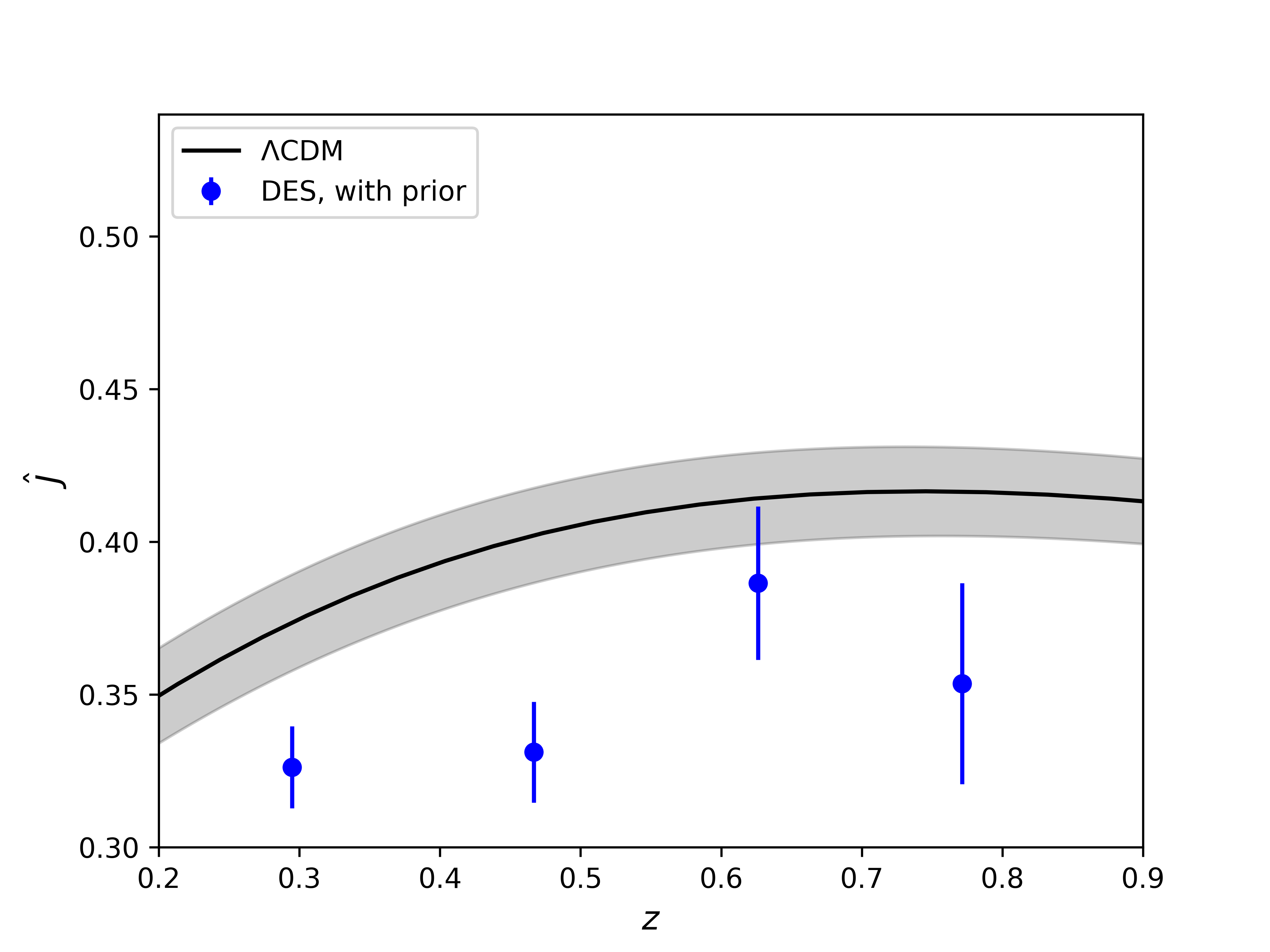
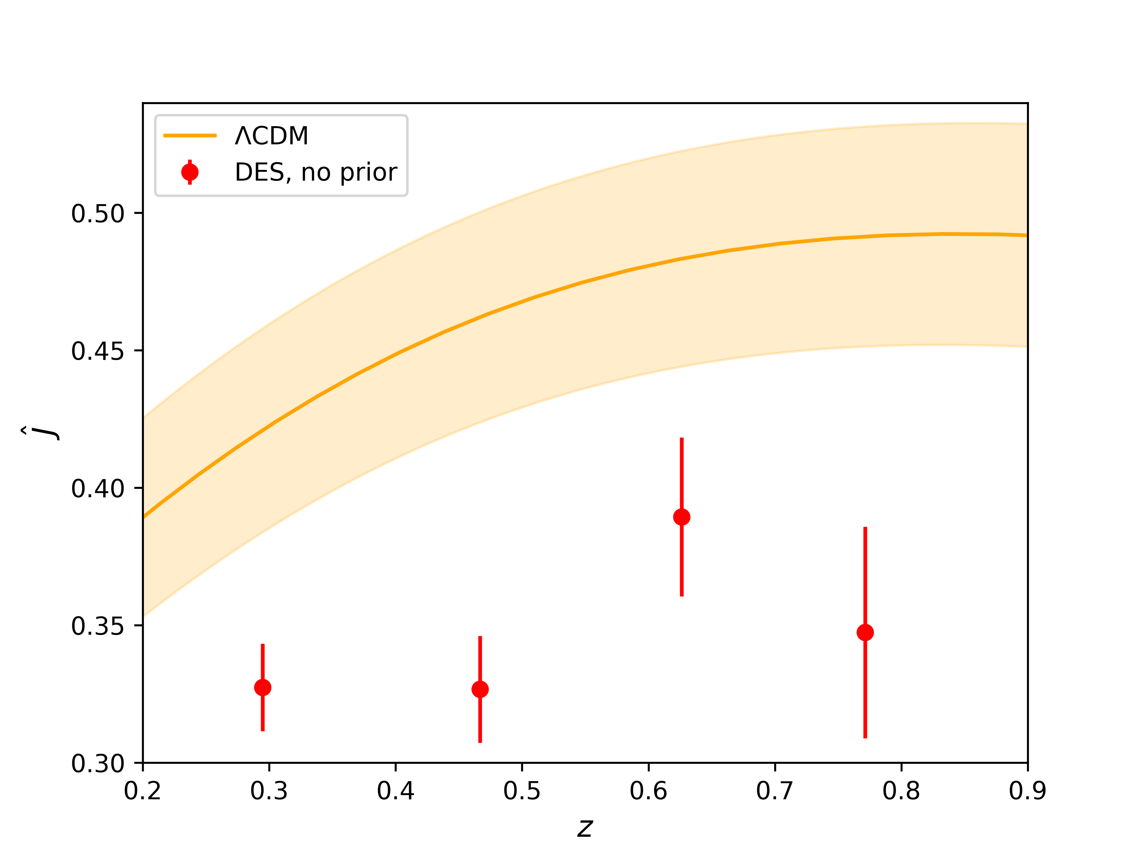
Figure 1: Measured values of $\hat{J}$ at the mean redshifts of the MagLim sample. The left panel shows the measurements assuming a prior from Planck on early time cosmological parameters. The right panel shows the measurements without any priors. The black and orange solid lines show the predictions for $\hat{J}$ in $\Lambda$CDM. The shaded regions indicate the 1$\sigma$ uncertainty on those predictions due to uncertainties in the primordial cosmological parameters.

Table 1: Mean values and 1$\sigma$ error bars for $\hat{J}(z_{i})$ in the four cases considered in our analysis: with and without Planck priors, with standard and pessimistic scale cuts.

	CMB prior		No prior
	Standard cuts	Pessimistic cuts	Standard cuts	Pessimistic cuts
$\hat{J}(z_{1})$	$0.326\pm 0.013$	$0.332\pm 0.025$	$0.327\pm 0.016$	$0.340\pm 0.027$
$\hat{J}(z_{2})$	$0.331\pm 0.017$	$0.326\pm 0.030$	$0.327\pm 0.019$	$0.331\pm 0.032$
$\hat{J}(z_{3})$	$0.387\pm 0.025$	$0.426\pm 0.057$	$0.389\pm 0.029$	$0.439\pm 0.058$
$\hat{J}(z_{4})$	$0.354\pm 0.033$	$0.361\pm 0.068$	$0.347^{+0.036}_{-0.040}$	$0.374\pm 0.071$

IV.1 Measurements of $\hat{J}$ using priors from Planck

In Fig. 1, left panel, we show the measured values of $\hat{J}$ with 1$\sigma$ error bars. We see that $\hat{J}$ is very well measured, with a precision of 4 to 9% in the four DES redshift bins (see also Table 1). This demonstrates the capacity of galaxy-galaxy lensing and galaxy clustering to significantly constrain the Weyl evolution in a fully model-independent way, i.e. without assuming any theory of gravity at late time. The measured values of $\hat{J}$ can then be compared with any model of interest. In Fig. 1, we also show the prediction for $\hat{J}$ in $\Lambda$CDM, with the cosmological parameters obtained through our cosmological analysis. The shaded region corresponds to the 1$\sigma$ uncertainty on the $\Lambda$CDM prediction due to the uncertainty in the measurement of the cosmological parameters. In the first and second redshift bins, the measurements of $\hat{J}$ are 2.3$\sigma$, respectively 3.1$\sigma$, below the $\Lambda$CDM predictions. In the highest two bins the measurements are compatible with $\Lambda$CDM (1.7$\sigma$ difference in the last bin).

Even though such a tension is not very significant, especially given that the measurements of $\hat{J}$ in the different bins are slightly correlated (see the joint constraints in Fig. 6, Appendix C), it is interesting to see at which redshifts the measurements are in tension with $\Lambda$CDM. In particular, Fig. 1 shows that the deviations from $\Lambda$CDM are localised at the first two redshift bins, and actually more prominent in the second one. This could hint either at a modification of gravity that may have more impact at low redshift, when the mechanism responsible for the acceleration of the Universe is in full play. Or it could be due to a (partially) incorrect modelling of non-linear effects, which are more important at low redshift. Alternatively, it could also be due to unknown systematic effects in the first two bins of the MagLim sample. Since there is an important difference between the measurements in the second and third bins, it would be interesting to obtain a measurement in between.

Until now, $\hat{J}$ has been measured in a fully model-independent way. It is however interesting to use these measurements to infer $\sigma_{8}(z=0)$ assuming $\Lambda$CDM. This value of $\sigma_{8}(z=0)$, which is inferred from the Weyl potential at low redshift, can then be compared with the value obtained from high redshift, i.e. from the cosmological parameters $\Omega_{\rm m},\Omega_{\rm b},n_{\rm s}$, and $A_{\rm s}$ that are constrained through the density power spectrum at $z_{*}=10$, the background functions $\mathcal{H}(z)$ and $\chi(z)$, and through Planck priors . In $\Lambda$CDM, $\hat{J}$ is given by

$$\hat{J}(z)=\Omega_{\rm m}(z)\frac{D_{1}(z)}{D_{1}(z=0)}\sigma_{8}(z=0)\,.$$ (8)

Combining the four measurements of $\hat{J}$, we can fit for $\sigma_{8}(z=0)$ at each point of the chain, and obtain its posterior distribution which we find to be close to Gaussian (see Fig. 7 in Appendix C). The mean and 1$\sigma$ errors are $\sigma^{\rm fit}_{8}(z=0)=0.74\pm 0.04$. In contrast, using the values of $\Omega_{\rm m},\Omega_{\rm b},n_{\rm s}$ and $A_{\rm s}$, we obtain $\sigma^{\rm cosmo}_{8}(z=0)=0.85\pm 0.03$, which is 2.5$\sigma$ higher than the value obtained from $\hat{J}$. With our method, we recover therefore the well-known result from the Year 3 DES data that high redshifts prefer a larger clustering amplitude than low redshifts. Moreover, we are able to pin-point this (mild) tension to the behaviour of the Weyl potential in the two lowest redshift bins of DES. Interestingly, the value of $\sigma_{8}(z=0)$ obtained from the early time cosmological parameters is slightly larger (by 1.3$\sigma$) in our analysis than when only Planck data are used: $0.85\pm 0.03$ versus $0.810\pm 0.007$. As we will see below, this tendency becomes even more prominent when no priors are imposed on the primordial cosmological parameters. Note that we obtain similar results if we use $\hat{J}$ to infer $S_{8}=\sigma_{8}\sqrt{\Omega_{\rm m}/0.3}$. In this case, the tension between the late time measurement of $S_{8}$ and the value obtained from early time cosmological parameters is 2.4$\sigma$.

In this analysis we have used priors on cosmological parameters from Planck coming from the temperature and the polarisation, but without lensing, since Planck constraints from lensing assume the validity of $\Lambda$CDM at late time. However, even if lensing is not included as an additional observable, it still affects the temperature power spectrum. One way to remove this information is to consider Planck analysis with an additional parameter $A_{\rm L}$ in front of the amplitude of the lensing contribution, and to marginalise over it. This effectively removes the constraining power of lensing on cosmological parameters, ensuring that those are only constrained by early time fluctuations. As a cross-check, we have redone our analysis, using these new priors from Planck. We find that the results barely change. The tension between the measured $\hat{J}$ and the $\Lambda$CDM prediction slightly decreases (e.g. from 3.1$\sigma$ to 2.7$\sigma$ in the second bin) due to the fact that Planck priors increase with this extra parameter $A_{\rm L}$.

Finally, we have redone our analysis using the sampler PolyChord instead of MultiNest. The mean values of $\hat{J}$ change by less than 0.5%. The errors however increase slightly, by $7-12\%$. The errors on cosmological parameters also increase by a similar amount ($5-9\%$), leading to a tension with $\Lambda$CDM predictions which is very slightly reduced: 2$\sigma$ in the first bin and 2.7$\sigma$ in the second bin, compared to 2.3$\sigma$ and 3.1$\sigma$ when using MultiNest.

Table 2: The values for $\sigma_{8}(z=0)$, in the cases with and without CMB priors, using the standard scale cuts. We compare the value fitted from $\hat{J}$ with the value obtained from the cosmological parameters.

	CMB prior		No prior
	From parameters	From $\hat{J}$	From parameters	From $\hat{J}$
$\sigma_{8}(z=0)$	$0.852\pm 0.027$	$0.741\pm 0.035$	$1.037\pm 0.093$	$0.780^{+0.064}_{-0.073}$

IV.2 Measurements of $\hat{J}$ without Planck prior

In the right panel of Fig. 1, we show the measured values of $\hat{J}$ when the cosmological parameters are left completely free to vary, i.e. without imposing a prior from Planck. We see that $\hat{J}$ can still be very well measured in this case: the errors increase by $\sim 20\%$ only (see Table 1). On the other hand, the errors on the cosmological parameters are 3 to 6 times larger when no priors are used. The primordial amplitude $A_{\rm s}$ and the Hubble parameter $h$ are the parameters that are the most degraded by removing the priors. This is not surprising, since in our framework cosmological parameters are only constrained by the primordial density power spectrum at $z_{*}=10$ and by the evolution of the background, namely $\mathcal{H}(z)$ and the comoving distance $\chi(z)$. All the information coming from the growth of structure and from the Weyl potential is encoded in the parameters $\hat{J}$ and $\hat{b}_{i}$ and does not contribute to the constraints on the cosmological parameters. The whole goal of our approach is indeed to assume that we do not know how the Weyl potential evolves at late time. The larger uncertainties in cosmological parameters lead to wider errors on the prediction for $\hat{J}$ in $\Lambda$CDM, as is clearly visible from Fig. 1.

We see that removing the priors actually slightly increases the tension between the measured $\hat{J}$ and the $\Lambda$CDM predictions, which is now $[2.3\sigma,3.1\sigma,1.9\sigma,2.6\sigma$] in the four bins. From Fig. 1, we see that this is due to the fact that the $\Lambda$CDM predictions for $\hat{J}$ increase when the prior is removed. This can be traced to an increase of the primordial amplitude $A_{\rm s}$ from $(2.14\pm 0.09)\times 10^{-9}$ to $3.04^{+0.55}_{-0.68}\times 10^{-9}$. Hence we see that DES data on their own prefer a high amplitude of perturbations at high redshift, followed by a growth of the Weyl potential slower than in $\Lambda$CDM at low redshifts. Again, this could hint to a modification of gravity that would slow down the growth of the Weyl potential at late time. More precisely, modifications of gravity can change the relation between density perturbations at $z_{*}=10$ which affect the lensing signal through $P_{\delta\delta}(z_{*})$, see Eq. (3), and the evolution of the Weyl potential at low redshift encoded in $\hat{J}$. The tension could also be due to an imperfect modelling of non-linearities, that would also affect the relation between the linear density power spectrum at $z_{*}$ and the evolution of the Weyl potential. Alternatively, it could be due to systematic effects. In any case, it is highly interesting that the tension remains when CMB data are not used at all.

The tension in $\hat{J}$ leads to a 2.2$\sigma$ tension between $\sigma_{8}$ extracted from the cosmological parameters: $\sigma^{\rm cosmo}_{8}(z=0)=1.04\pm 0.09$, and $\sigma_{8}$ extracted from $\hat{J}$ assuming $\Lambda$CDM: $\sigma^{\rm fit}_{8}(z=0)=0.78\pm 0.07$. The very large value of $\sigma^{\rm cosmo}_{8}$ is directly related to the large value of $A_{\rm s}$. The $\sigma_{8}$ tension is sometimes referred to as a tension between CMB data and weak lensing data. Here, we see that it is truly a tension between low and high redshift that is encoded into DES data on their own. Translating the constraints on $\sigma_{8}(z=0)$ to constraints on $S_{8}$ we find that the tension is slightly larger, of 2.7$\sigma$. We summarise the values of $\sigma_{8}(z=0)$ obtained in various cases in Table 2.

Finally, we have looked at the degeneracies of $\hat{J}$ with the nuisance parameters. We find that $\hat{J}$ is degenerated with the stretch of the photometric redshift distribution of the lens sample (see Fig. 8 in Appendix C). This stretch is added as a free parameter in the baseline DES analysis, together with a shift, to account for photometric redshift systematic effects DES:2021bpo . The stretch and the shift are calibrated using clustering with spectroscopic surveys DES:2020sjz , leading to tight priors on these parameters. We find that a large value of the stretch, i.e. a distribution which is more spread, can be counterbalanced by smaller values of $\hat{J}$, and vice-versa. This can be understood from Eq. (3): increasing the width of $n_{i}(z)$ tends to increase the values of the integral over $z$, due to the lensing kernel $(\chi(z)-\chi^{\prime}(z^{\prime}))/(\chi(z)\chi^{\prime}(z^{\prime}))$, which increases when $\chi(z)$ is allowed to take smaller values. In order to have $\hat{J}$ in 1$\sigma$ agreement with $\Lambda$CDM predictions in the second bin, we would need a stretch of 0.94, which is in clear tension with the values obtained from calibration: $1.306\pm 0.093$ (the mean value from our analysis is $1.239\pm 0.076$). Table 3 in Appendix A summarises the mean values and error bars for all nuisance parameters.

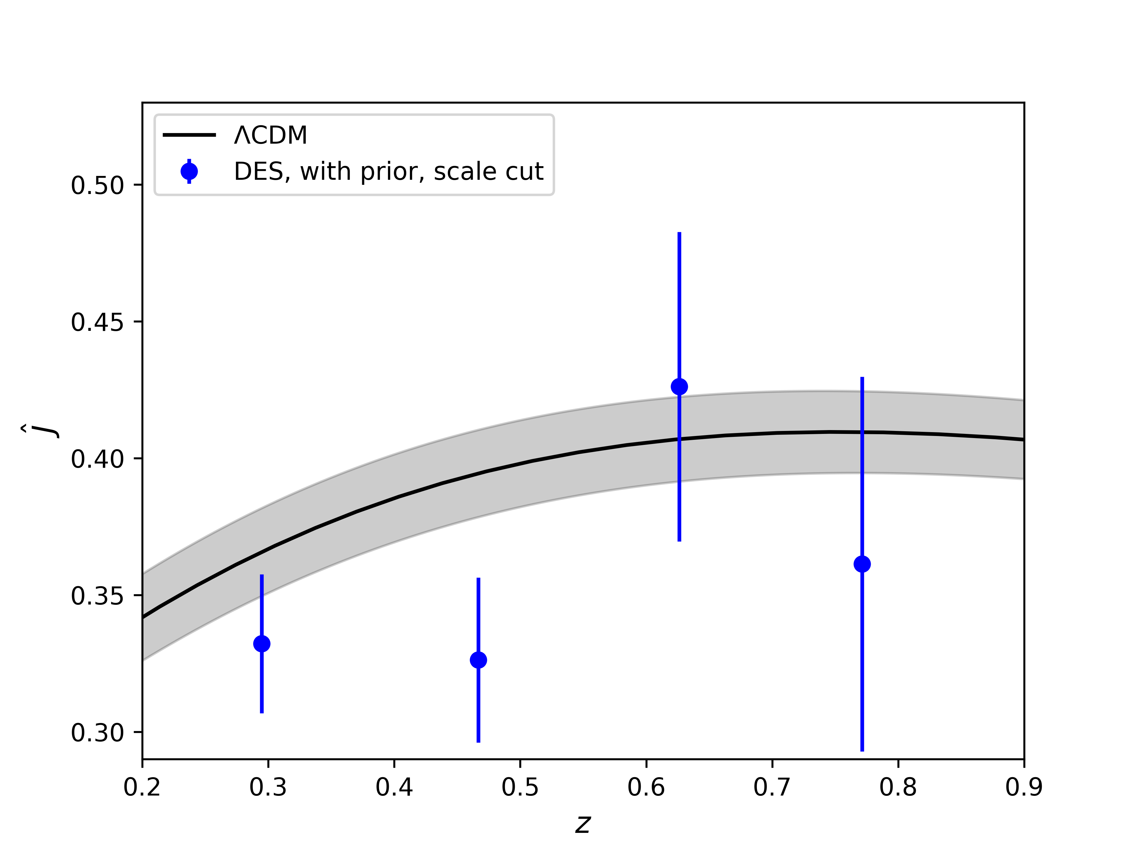
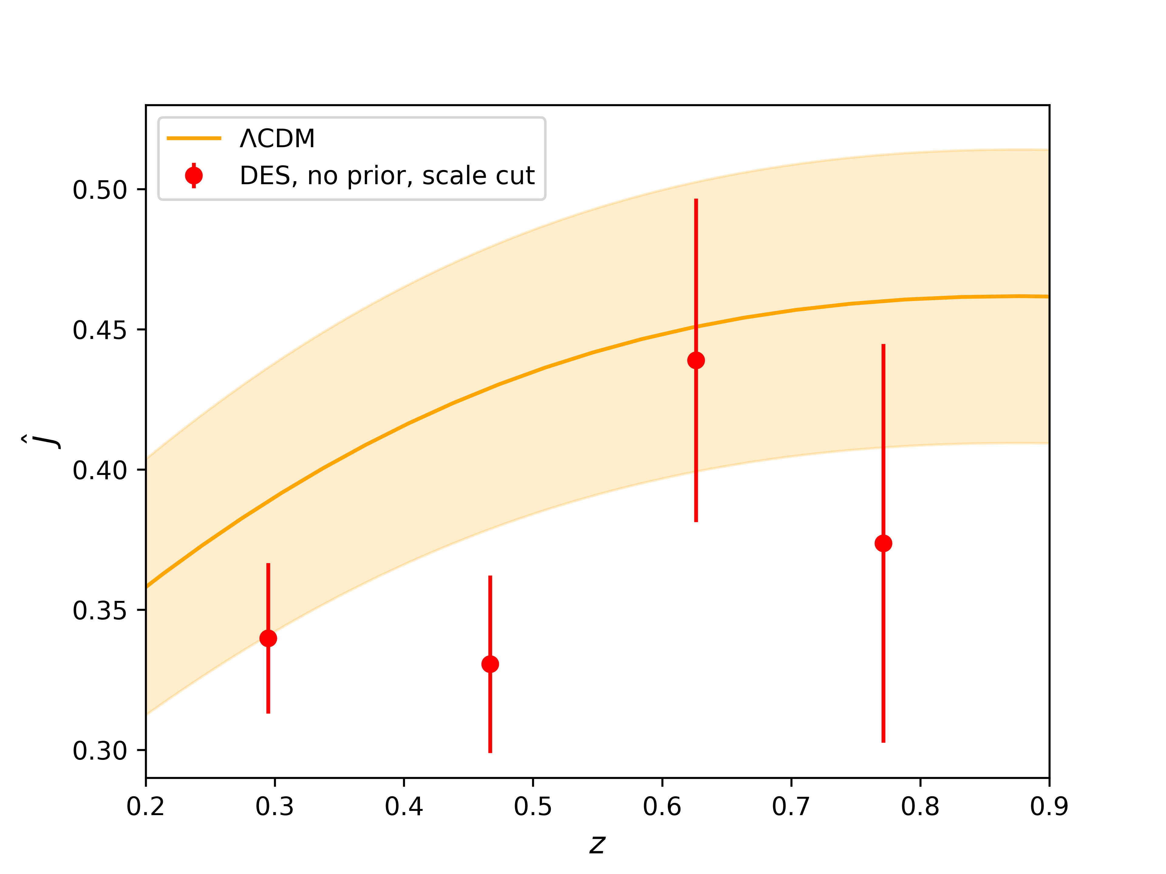
Figure 2: Measured values of $\hat{J}$ at the mean redshifts of the MagLim sample, using more stringent scale cuts. The left panel shows the measurements assuming a prior from Planck on early time cosmological parameters. The right panel shows the measurements without any priors. The black and orange solid lines show the predictions for $\hat{J}$ in $\Lambda$CDM. The shaded regions indicate the 1$\sigma$ uncertainty on those predictions due to uncertainties in the primordial cosmological parameters.

IV.3 Measurements of $\hat{J}$ with more stringent non-linear scale cuts

As discussed in Section III, we have implemented more stringent scale cuts to remove further the impact of non-linear scales. The results for $\hat{J}$ are shown in Fig. 2 for the analysis with Planck priors (left panel) and without (right panel). We see that the measurements of $\hat{J}$ are significantly degraded: the errors increase by roughly a factor 2. This is not surprising since removing scales reduces the available amount of information needed to measure $\hat{J}$. The errors on the $\Lambda$CDM prediction also increase due to the scale cut, in the case without prior, but only by 30%. Interestingly, the mean values of $\hat{J}$ are almost not affected by removing scales and are still below the $\Lambda$CDM predictions. However, the increase in the error bars significantly reduces the tension with $\Lambda$CDM predictions: only the second bin is still 2$\sigma$ away from the $\Lambda$CDM prediction in the case with prior (1.6$\sigma$ without prior). A comparison of the measurements of $\hat{J}$ with standard and pessimistic scale cuts is provided in Table 1.

IV.4 Comparison with binned $\sigma_{8}(z)$ analysis of DES

It is worth comparing our results with the binned $\sigma_{8}(z)$ analysis of DES DES:2022ygi . In this analysis, $\Lambda$CDM is assumed to be correct, and four additional free parameters, $A_{i}^{P_{\rm lin}}$, are added in front of the density power spectrum in the four redshift bins of the lenses. The parameter in the first bin is then fixed to 1 (to break the degeneracy with the primordial amplitude $A_{\rm s}$), whereas the other three are constrained by the data. This analysis differs from ours in the sense that it is a consistency check of $\Lambda$CDM. If the parameters are found to be different from 1 in any of the bins, then $\Lambda$CDM is inconsistent. However, this analysis does not permit a determination of the origin of the tension. In particular, since $\Lambda$CDM is assumed to be correct, the Weyl potential is related to the matter density fluctuation using GR. As a consequence, the angular power spectra are all sensitive to the matter power spectrum, which is multiplied by a unique parameter $A_{i}^{P_{\rm lin}}$ (per bin). In reality however, the clustering angular power spectrum depends on the density-density correlation; the galaxy-galaxy lensing angular power spectrum depends on the density-Weyl correlation; and the shear angular power spectrum depends on the Weyl-Weyl correlation. Modifications of gravity are not expected to modify the evolution of the density and the evolution of the Weyl potential in the same way. Therefore, encoding those into a single parameter may not be optimal. Of course, as explained in DES:2022ygi , the goal of such a consistency check is not to model modified gravity, but rather to assess the consistency of $\Lambda$CDM. However, the fact that one has only one parameter per bin introduces an artificial mixing between this parameter and the galaxy bias, which could in principle reduce the signature of modified gravity. Deviations from GR in the Weyl potential would indeed, in this framework, lead to modifications of the parameters $A_{i}^{P_{\rm lin}}$, which would artificially change the clustering power spectrum as well (since $A_{i}^{P_{\rm lin}}$ multiplies all spectra). If the matter density is not modified, or if it is modified in a different way than the Weyl potential, this will lead to inconsistencies in the modelling that may be minimised by artifically decreasing deviations in $A_{i}^{P_{\rm lin}}$ and changing the bias or other cosmological parameters. In contrast, with our modelling, any deviation in the Weyl potential would be automatically visible in the measurement of $\hat{J}$, while deviations in the growth of the density would affect the parameters $\hat{b}_{i}(z)=b_{i}(z)\sigma_{8}(z)$.

A direct comparison of our results with the binned $\sigma_{8}(z)$ results is not possible, since the assumptions are different. However, from Fig. 11 and 12 of DES:2022ygi , one can see that when using only DES data, $\sigma_{8}$ tends to be lower than predicted by Planck using $\Lambda$CDM, at all redshifts. Combining with Planck increases the values, bringing them back towards the $\Lambda$CDM predictions. In our case, we find that starting with a power spectrum consistent with Planck at high redshift, and letting the evolution free at low redshift, leads to a Weyl evolution below $\Lambda$CDM predictions. As for the binned $\sigma_{8}(z)$ analysis, this trend is not very significant. However, the main difference is that in the second bin we have a value which is 3.1$\sigma$ below the $\Lambda$CDM prediction. This is not in contradiction with the results of the binned $\sigma_{8}(z)$ analysis, which does not see such a feature when DES and Planck are combined. By assuming $\Lambda$CDM to be valid and fixing $A_{1}^{P_{\rm lin}}=1$ in the lowest bin, the constraints from different bins are not truly independent. In particular, a deviation in one bin may lead to slightly different values of the $\Lambda$CDM parameters, which in turn will artificially influence the value of $A_{i}^{P_{\rm lin}}$ in the other bins. Moreover, the linear galaxy bias can also reabsorb part of the deviation. In our framework this is not the case: a deviation in one redshift bin does not influence the measurements in the other bins. The correlations between $\hat{J}$ in different bins is purely physical, only due to the evolution of the Weyl potential. From this we see that identifying the quantities that are truly measured by the data helps to correctly pin-point where tensions come from.

IV.5 Measurements of $\hat{J}$ using the redMaGiC lens sample

In our analysis we have used the MagLim lens sample, which is the fiducial sample of DES. It is, however, interesting to see how the results change if we use the redMaGiC sample instead. For our baseline scenario (with Planck priors and standard scale cuts), we find that the measured $\hat{J}$ using redMaGiC are systematically below the $\Lambda$CDM predictions (see Fig. 5 and Table 4 in Appendix B). The tension with $\Lambda$CDM in the five bins of redMaGiC are $[2.9,3.2,2.6,2.3,3.1]\sigma$. Starting from these measurements and assuming the validity of $\Lambda$CDM, we find that the inferred value for $\sigma_{8}$ at late time is $\sigma^{\rm fit}_{8}(z=0)=0.63\pm 0.04$, which is 4.1$\sigma$ below the value inferred from early time cosmological parameters: $\sigma^{\rm cosmo}_{8}(z=0)=0.82\pm 0.03$.

This non-negligible tension with respect to $\Lambda$CDM predictions is in agreement with the results of the DES Collaboration, who found that $\sigma_{8}$ measured from galaxy-galaxy lensing and galaxy clustering is significantly lower using redMaGiC than MagLim DES:2021zxv . To account for this, an artificial parameter $X_{\rm lens}$ was introduced, encoding a difference in the galaxy bias obtained from galaxy clustering and the bias obtained from galaxy-galaxy lensing. This parameter was found to be in 5$\sigma$ tension with its expected value of 1, reflecting the fact that the galaxy clustering amplitude was systematically larger than the galaxy-galaxy lensing amplitude DES:2021zxv ; DES:2021wwk . This is fully in line with our findings: leaving the function $\hat{J}$ free, we find that the data prefer a low value of $\hat{J}$ consistent with a galaxy-galaxy lensing correlation lower than in $\Lambda$CDM. The DES Collaboration relates the low value of $X_{\rm lens}$ to systematic effects due to the selection of galaxies in the redMaGiC sample. Such systematic effects would bias our measurements of $\hat{J}$, which is degenerated with the galaxy bias in the galaxy-galaxy lensing signal. One way to investigate this would be to measure $\hat{J}$ from shear-shear correlations and see if the results are consistent. We defer this to a future analysis.

V Modified gravity

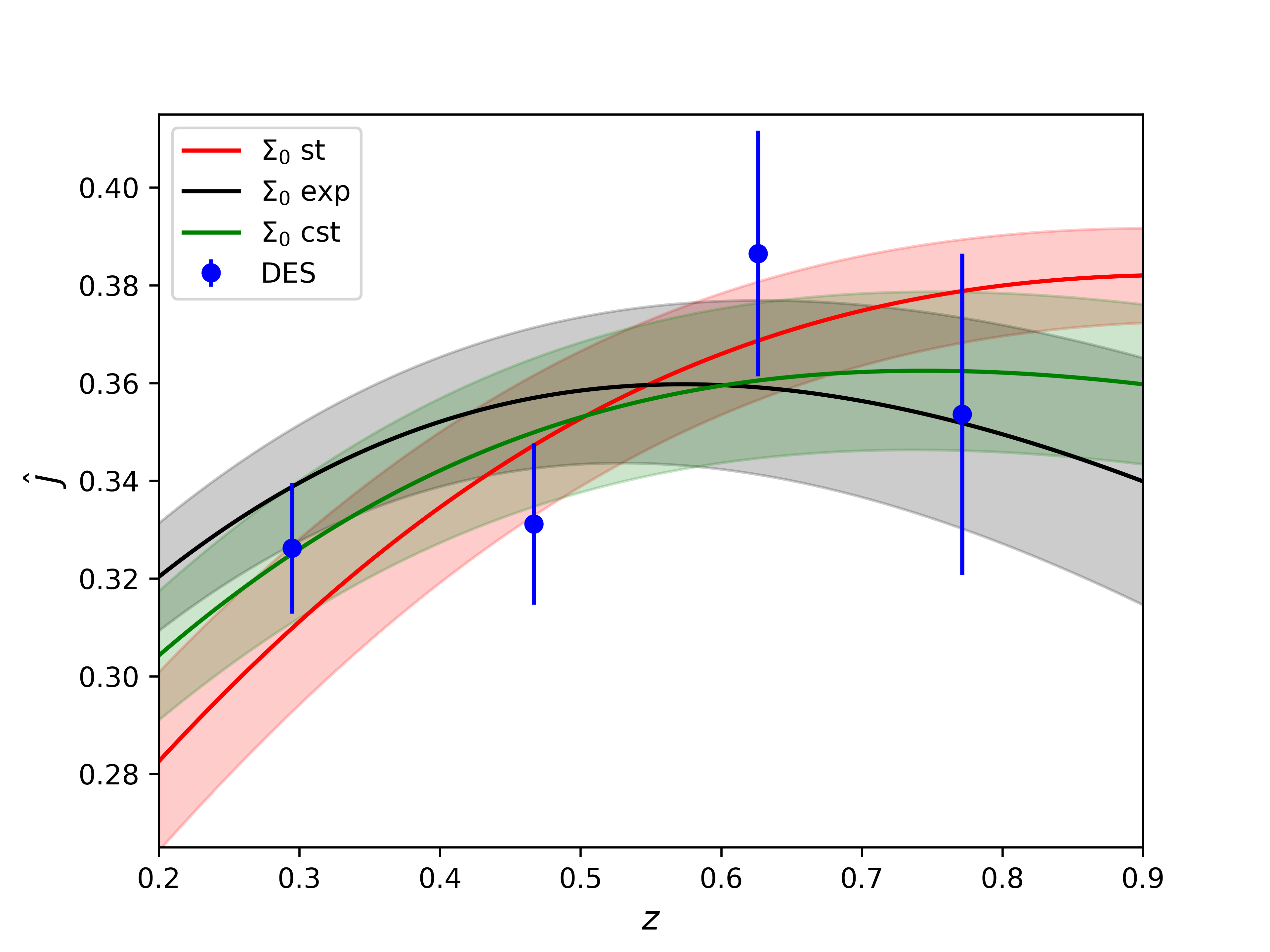
Figure 3: Predictions for $\hat{J}$ for modified gravity models with $\Sigma\neq 1$ and $\mu=1$. We show the mean value together with the 1$\sigma$ uncertainty for the three choices of time evolution (standard, constant, and exponential) described in the text. The measurements correspond to our baseline, using Planck priors and with standard scale cuts.

The measurements of $\hat{J}$ are fully model-independent and they can therefore be compared with predictions in any theory of gravity (as long as GR is recovered at high redshift), without having to redo the analysis. Here, as an illustration, we consider two cases: A) the phenomenological $\mu-\Sigma$ extensions of gravity; and B) Horndeski theories, concentrating on a few specific cases.

V.1 $\mu-\Sigma$ modifications of gravity

The phenomenological parameters $\mu$ and $\Sigma$ encode deviations from GR in the relation between the metric potentials and the matter density fluctuations,

$$k^{2}\Psi=-4\pi\mu(a,k)Ga^{2}\rho\delta\,\quad\mbox{and}\quad k^{2}\Psi_{W}=-4\pi\Sigma(a,k)Ga^{2}\rho\delta\ .$$ (9)

In GR, $\mu=\Sigma=1$. These parameters affect $\hat{J}$ in the following way,

$$\hat{J}(z)=\Sigma(z)\Omega_{\rm m}(z)D_{1}(z)\frac{\sigma_{8}(z_{*})}{D_{1}(z_{*})}\,,$$ (10)

where as before we have neglected the dependence in $k$, as is usually done in the literature, see e.g. DES:2022ygi (both due to the fact that current data are not constraining enough to probe a possible scale-dependence in $\mu$ and $\Sigma$, and that in many models of modified gravity the scale-dependence is negligible for sub-horizon scales). $\hat{J}$ depends directly on $\Sigma$, but it also depends on $\mu$ through the evolution of $D_{1}(z)$. Eq. (10) underlines the difference between measuring $\hat{J}$, and measuring $\mu$ and $\Sigma$. $\hat{J}$ can be measured from lensing data on their own. The parameters $\mu$ and $\Sigma$, on the other hand, cannot be measured separately from lensing only, since their impact on $\hat{J}$ is fully degenerated. To determine if $\mu$ and $\Sigma$ are consistent with GR, it is therefore necessary to include other measurements, like RSD. Moreover, in order to constrain $\mu$ from RSD, one has to assume the validity of Euler’s equation for dark matter. The growth of structure is indeed not only affected by $\mu$, but also by additional forces or interactions affecting dark matter SvevaNastassiaCamille ; Bonvin:2022tii . As a consequence, the constraints on $\Sigma$ from lensing also rely on the validity of Euler’s equation. In contrast, $\hat{J}$ can be measured without any assumptions on the behaviour of dark matter. Finally, we see from Eq. (10) that $\hat{J}$ depends directly on the redshift evolution of $\mu$ and $\Sigma$, which is unknown. In particular, $\hat{J}$ depends on $\mu(z)$ through a second order evolution equation, which requires knowledge of $\mu(z)$ not only at the redshift of the analysis, but also at all redshifts above it.

In practice, we find that $\hat{J}$ is much more sensitive to $\Sigma$ than to $\mu$. Here, we aim to investigate the constraining power of $\hat{J}$, without the inclusion of additional RSD data. Therefore, as illustration, we choose $\mu=1$ (as in GR) and we infer $\Sigma$ from $\hat{J}$. We consider 3 different choices of time evolution, encoded through

$$\Sigma(z)=1+\Sigma_{0}g(z)\,,$$ (11)

with 1) the standard evolution that has been used in the DES analysis DES:2022ygi and in Planck analysis Planck:2018vyg : $g(z)=\Omega_{\Lambda}(z)$; 2) no evolution: $g(z)=1$ for $z\in[0,1]$ and 0 elsewhere; and 3) an exponential evolution: $g(z)=\exp(1+z)$ for $z\in[0,1]$ and 0 elsewhere. The first case is motivated by the fact that deviations from GR are linked to the accelerated expansion of the Universe, and are therefore expected to decay proportionally to the amount of dark energy. The second and third cases are not physically motivated time evolutions, but they allow us to explore the sensitivity of the data to various behaviours, drastically different from each other.

At each point of the chain, we fit for $\Sigma_{0}$ using Eq. (10), combining the four measurements of $\hat{J}$. The value $\sigma_{8}(z_{*})$ is computed at each point from the cosmological parameters using CAMB  Lewis:1999bs . The posteriors for $\Sigma_{0}$ are very close to Gaussian for the three cases, with mean and 1$\sigma$ errors given by: $\Sigma_{0}^{\rm st}=-0.24\pm 0.09$ (standard evolution), $\Sigma_{0}^{\rm cst}=-0.14\pm 0.05$ (no evolution) and $\Sigma_{0}^{\rm exp}=-0.03\pm 0.01$ (exponential evolution). In Fig. 3 we show the predicted $\hat{J}(z)$ (mean and $1\sigma$ error bands) for the three models, compared with the measured $\hat{J}$ in the baseline case (with Planck priors and standard scale cuts). In the three cases, a negative value of $\Sigma_{0}$ decreases $\hat{J}$ with respect to $\Lambda$CDM, leading to a better agreement with the data (at the cost of one extra parameter though). The reduced chi-squared of the three models is very similar: 1.6 for the standard evolution and the constant case, and 1.5 for the exponential evolution. This shows that the data are not able to discriminate between the different time evolutions, as is clear from Fig. 3. The coming generation of surveys has clearly the potential to help, by adding measurements at lower and higher redshifts and reducing the error bars. Here we also see the strong advantage of our method: by first measuring $\hat{J}$ without assuming any model and then comparing with the predictions in modified gravity, we can easily understand and test the impact of different assumptions about the time evolution.

V.2 Horndeski theories and a non-minimal coupling of CDM

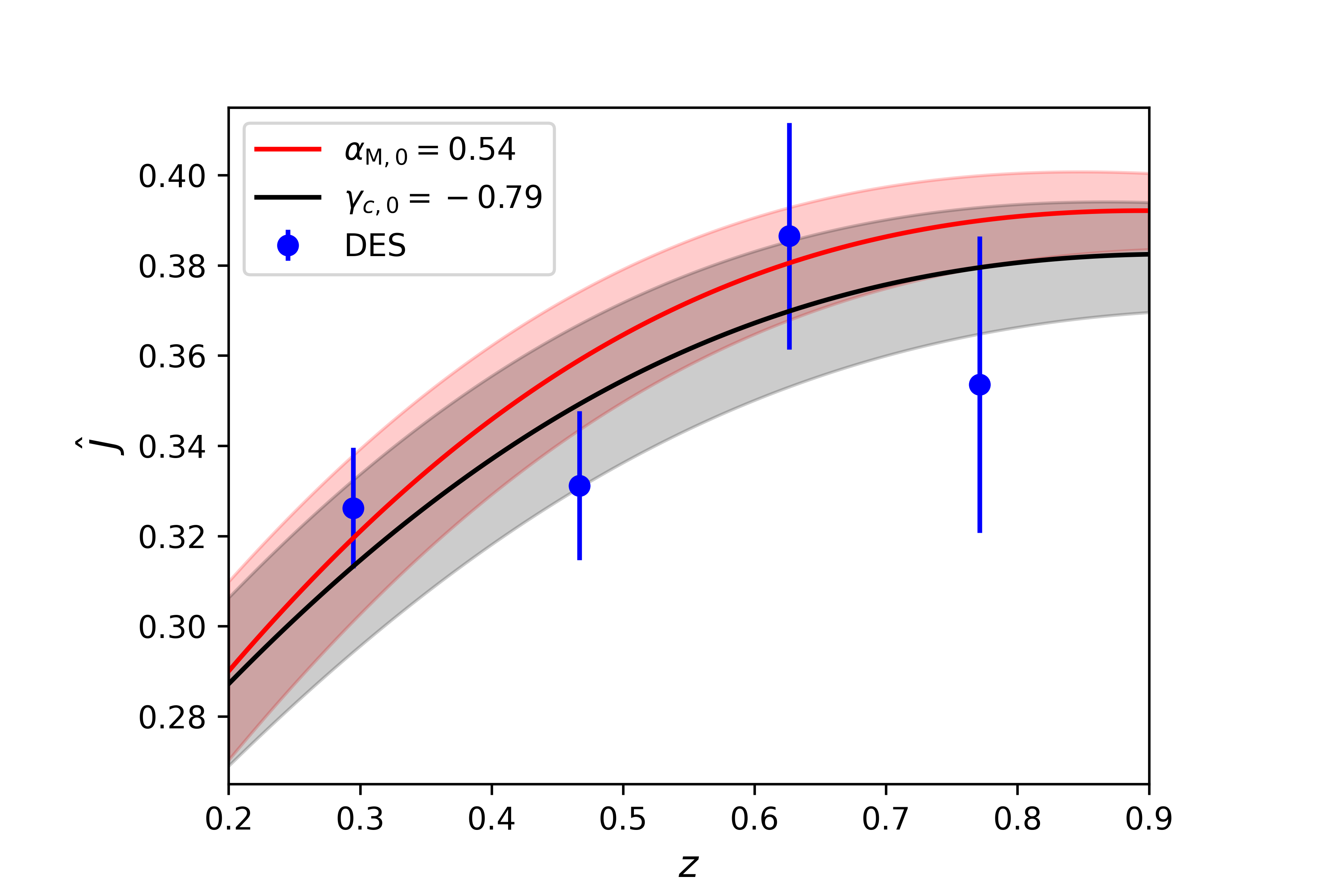
Figure 4: Best-fit and $1\sigma$ bands for a Horndeski model with $\alpha_{\rm M}=2\alpha_{\rm B}$ (red) and a model with a non-minimal coupling, $\gamma_{c}\neq 0$, of CDM to the metric (black). In both cases, all other modified gravity parameters are assumed to maintain their GR values.

Besides these phenomenological modifications of GR, we also consider Horndeski models Horndeski1974 , which constitute the most general class of Lorentz-invariant scalar-tensor theories with second-order equations of motion. In the regime of linear cosmological perturbations, this broad class of theories can be expressed in an effective theory approach by a limited number of parameters Bellini:2014fua , including the running of the Planck mass $\alpha_{\rm M}$ and the braiding $\alpha_{\rm B}$. Following the approach of Castello:2023zjr ; Gleyzes:2015pma ; Gleyzes:2015rua , we additionally allow for dark matter to be non-minimally coupled to the scalar field, since the weak equivalence principle has not been tested for dark matter. While theoretically easier to interpret, since the modifications enter directly at the level of the Lagrangian, Horndeski models with a non-minimal coupling of CDM add more complexity compared to the phenomenological $\mu-\Sigma$ modifications. In particular, they influence the background evolution of $\mathcal{H}(z)$ along with the perturbations. As previously mentioned, relaxing the assumption of the background evolution of $\Lambda$CDM would necessitate the inclusion of further data sets, which is beyond the scope of this work. Instead, for simplicity we neglect the impact on the background evolution and only constrain the parameters through their impact on $\hat{J}$. As such, our constraints should be seen as an illustration of the capability of this model type to explain a $\hat{J}$ measurement different from the $\Lambda$CDM prediction, rather than a full analysis of the models.

We focus on two specific cases: first, we consider the case where $\alpha_{\rm B}=\alpha_{\rm M}/2$ can differ from zero, and dark matter is minimally coupled to the scalar field, $\gamma_{c}=0$ (see e.g. Castello:2023zjr for more detail on these parameters). This special relation between $\alpha_{\rm M}$ and $\alpha_{\rm B}$ is recovered e.g. in Brans-Dicke theories Brans:1961sx ; Sawicki:2012re and some $f(R)$ models  Carroll:2003wy ; Song:2006ej ; Carroll:2006jn ; Vollick:2003aw . Second, we investigate the case with a non-minimal coupling of dark matter, $\gamma_{c}\neq 0$, while all other parameters are kept to their GR value. As before, we need a time evolution for the parameters, which we choose to be $g(z)=\Omega_{\Lambda}(z)$ as usually considered for Horndeski models. For both cases, we consider the baseline analysis, with Planck priors and standard scale cuts.

To find $\alpha_{\rm M,0}$ and $\gamma_{\rm c,0}$ we can use Eq. (10), which is also valid in Horndeski theories. For each value of the parameters, we can compute $\Sigma(z_{i})=\mu(z_{i})(1+\eta(z_{i}))$, using the relations between the model parameters $(\alpha_{\rm M},\alpha_{\rm B},\gamma_{c})$ and the phenomenological parameters $(\mu,\eta)$ stated in Appendix A of Castello:2023zjr . We then use the EF-TIGRE code  developed in Castello:2023zjr to obtain $\Omega_{\rm m}(z_{i})$ and $D_{1}(z_{i})/D_{1}(z_{\ast})$. In addition to their dependence on $\alpha_{\rm M,0}$ and $\gamma_{\rm c,0}$, these quantities depend also on the primordial cosmological parameters. However, since it is computationally expensive to solve the system of differential equations at each point of the chain, we solve it instead for the mean values of the primordial cosmological parameters obtained from our analysis. Similarly, we compute the mean value of $\sigma_{8}(z_{*})$ using CAMB. With this, we can compute $\hat{J}(z_{i})$ using Eq. (10). We then fit for $\alpha_{\rm M,0}$, respectively for $\gamma_{c,0}$, using the mean values for the four measured $\hat{J}$ and their covariance from our baseline analysis. Since we do not fit for $\alpha_{\rm M,0}$ and $\gamma_{c,0}$ at each point of the chain, we do not have posteriors for these quantities. We can, however, compute the 1$\sigma$ error bars by propagating the errors on the primordial parameters. In principle, the way in which the errors on $\Omega_{\rm m}$ and $\Omega_{\rm b}$ at initial epoch propagate into the errors on $\Omega_{\rm m}(z_{i})$ and $D_{1}(z_{i})/D_{1}(z_{\ast})$ depends on the values of the modified gravity parameters. For simplicity, we assume that they are the same as in $\Lambda$CDM.

For the two specific models, we obtain $\alpha_{\rm M,0}=2\alpha_{\rm B,0}=0.54^{+0.19}_{-0.18}$ and $\gamma_{c,0}=-0.79^{+0.28}_{-0.33}$. We illustrate our results in Fig. 4, which shows that both cases lead to a very similar functional behaviour of $\hat{J}(z)$. We conclude that both $\alpha_{\rm M}=2\alpha_{\rm B}>0$ as well as $\gamma_{c}<0$ can decrease the amplitude of the Weyl potential at late time, leading to predicted values of $\hat{J}(z)$ in line with the measured data. However, from measurements of $\hat{J}(z)$ alone it is not possible to distinguish between modifications of gravity encoded in $\alpha_{\rm M}$ and $\alpha_{\rm B}$, and a breaking of the weak equivalence principle for CDM given a non-minimal coupling $\gamma_{c}<0$. Nevertheless, the observable $\hat{J}$ provides an excellent test of the $\Lambda$CDM model. A combination with other observables, in particular gravitational redshift, will allow to break degeneracies between different physical effects Castello:2023zjr .

VI Conclusion

In this paper, we have performed the first measurement of the Weyl potential from galaxy-galaxy lensing. Using data from DES, we were able to measure the function $\hat{J}(z)$, which encodes the evolution of the Weyl potential, with a precision of 4 to 9% in the four bins of the MagLim lens sample. We found that the measured values in the two lowest bins are in mild tension with the $\Lambda$CDM predictions. Imposing more stringent scale cuts does not impact the mean values of $\hat{J}$, which remain below the $\Lambda$CDM predictions. However, it degrades the constraints by a factor of 2, thus decreasing the tension.

One remarkable feature of our method is that it allows us to separate the information coming from the matter density fluctuations (which we do not use to constrain gravity, since it is fully degenerated with the galaxy bias) from the information coming from the Weyl potential. The latter purely encodes the growth of the spatial and temporal distortions of the geometry, and is therefore independent of the galaxy bias. Moreover, our method does not rely on any assumption about the redshift evolution of $\hat{J}$: the function is directly measured in each bin of the survey.

Our measurements allow us to pin-point the $\sigma_{8}$ tension to the fact that the Weyl potential is smaller than predicted in $\Lambda$CDM in the first two bins of the DES data. Surprisingly, we found that the tension remains even when no priors from the CMB are used. DES data on their own prefer a Universe with a high initial value of the primordial potential (higher than measured by Planck) followed by a slower growth at late time. Further investigation to understand the origin of this behaviour is needed. In particular, it would be interesting to redo the analysis changing the settings to the ones used in the new combined analysis of DES and KiDS Kilo-DegreeSurvey:2023gfr (which found a decrease of the $\sigma_{8}$ tension) to see how this impacts the measurements of $\hat{J}$. Moreover, having measurements of $\hat{J}$ between the second and third bin of DES, where the deviation suddenly appears could help understand the origin of the tension. Surveys like Euclid and LSST will be of crucial importance for this.

More generally, our method allows us to compare the measurements of $\hat{J}$ with predictions in any theory of gravity that recovers GR at high redshift. Since the measurements are model-independent, the method allows for various tests of the theory of gravity in an efficient way. One can for example easily change the time evolution of the parameters of the theory, without having to reanalyse the data for each case. Using the $\mu-\Sigma$ parameterisation of modified gravity, we have shown that current data are not constraining enough to differentiate between different time evolutions. However, future surveys like Euclid and LSST are expected to provide sufficiently tight constraints (at the level of $0.1-1\%$ for $z\in[0.25,2.1]$ for LSST Tutusaus:2022cab ) over a wider redshift range, to allow for much more stringent tests.

In a forthcoming paper, we will study how the evolution of the Weyl potential can be combined with measurements of the growth rate of structure, to test the relation between these two fundamental quantities in our Universe.

Data availability statement

All the data used in this analysis have been produced and publicly released by the DES Collaboration DES:2021wwk . It is accessible through the CosmoSIS software Zuntz:2014csq in https://cosmosis.readthedocs.io/en/latest/.

Appendix A List of cosmological and nuisance parameters

In Table 3, we list the mean values and 1$\sigma$ errors that we obtain for all cosmological parameters and nuisance parameters. We show the results for the baseline analysis, i.e. using CMB priors and standard scale cuts, and the case where we use only DES data (also with standard scale cuts).

Table 3: Mean values and 1$\sigma$ errors for the cosmological parameters and nuisance parameters obtained from the analysis with and without CMB priors. The two cases are for standard scale cuts.

		CMB prior	No prior
Matter density	$\Omega_{\rm m}$	$0.328\pm 0.011$	$0.292^{+0.027}_{-0.036}$
Baryon density	$\Omega_{\rm b}$	$0.0490\pm 0.0020$	$0.0424^{+0.0043}_{-0.011}$
Hubble parameter	$h$	$0.679\pm 0.016$	$0.728\pm 0.086$
Amplitude $\times 10^{9}$	$A_{\rm s}$	$2.137\pm 0.094$	$3.04^{+0.55}_{-0.68}$
Spectral index	$n_{s}$	$0.965\pm 0.012$	$0.986^{+0.078}_{-0.032}$
Bias $z_{1}$	$\hat{b}_{1}$	$0.953\pm 0.033$	$0.962\pm 0.041$
Bias $z_{2}$	$\hat{b}_{2}$	$1.022\pm 0.036$	$1.059\pm 0.049$
Bias $z_{3}$	$\hat{b}_{3}$	$1.006^{+0.033}_{-0.029}$	$1.038\pm 0.043$
Bias $z_{4}$	$\hat{b}_{4}$	$0.906\pm 0.024$	$0.937\pm 0.038$
Shear calibration	$m^{1}$	$-0.0060\pm 0.0085$	$-0.0060\pm 0.0087$
Shear calibration	$m^{2}$	$-0.0206\pm 0.0073$	$-0.0203\pm 0.0074$
Shear calibration	$m^{3}$	$-0.0244\pm 0.0070$	$-0.0243\pm 0.0069$
Shear calibration	$m^{4}$	$-0.0363\pm 0.0070$	$-0.0365\pm 0.0071$
Intrinsic alignment	$A_{\rm IA}$	$0.226^{+0.066}_{-0.086}$	$0.264^{+0.077}_{-0.087}$
Intrinsic alignment	$\alpha_{\rm IA}$	$-1.7^{+1.4}_{-2.4}$	$-0.7^{+1.9}_{-2.4}$
Lens photo-$z$ shift $z_{1}$	$\Delta z_{l}^{1}$	$-0.0089\pm 0.0058$	$-0.0094\pm 0.0060$
Lens photo-$z$ shift $z_{2}$	$\Delta z_{l}^{2}$	$-0.0269^{+0.0075}_{-0.0086}$	$-0.0285\pm 0.0085$
Lens photo-$z$ shift $z_{3}$	$\Delta z_{l}^{3}$	$-0.0020\pm 0.0054$	$-0.0013\pm 0.0055$
Lens photo-$z$ shift $z_{4}$	$\Delta z_{l}^{4}$	$-0.0067\pm 0.0056$	$-0.0063\pm 0.0057$
Lens photo-$z$ stretch $z_{1}$	$\sigma z_{l}^{1}$	$0.978\pm 0.057$	$0.978\pm 0.058$
Lens photo-$z$ stretch $z_{1}$	$\sigma z_{l}^{1}$	$1.211^{+0.071}_{-0.055}$	$1.239\pm 0.076$
Lens photo-$z$ stretch $z_{1}$	$\sigma z_{l}^{1}$	$0.888\pm 0.048$	$0.891\pm 0.050$
Lens photo-$z$ stretch $z_{1}$	$\sigma z_{l}^{1}$	$0.930\pm 0.044$	$0.931\pm 0.044$
Source photo-$z$ shift $z_{1}$	$\Delta z_{s}^{1}$	$0.0098\pm 0.015$	$0.0097\pm 0.015$
Source photo-$z$ shift $z_{2}$	$\Delta z_{s}^{2}$	$-0.0167^{+0.010}_{-0.0064}$	$-0.0160^{+0.0096}_{-0.0073}$
Source photo-$z$ shift $z_{3}$	$\Delta z_{s}^{3}$	$-0.0190\pm 0.0076$	$-0.0198\pm 0.0074$
Source photo-$z$ shift $z_{4}$	$\Delta z_{s}^{4}$	$0.008\pm 0.014$	$0.009\pm 0.014$

Appendix B Results using the redMaGiC lens sample

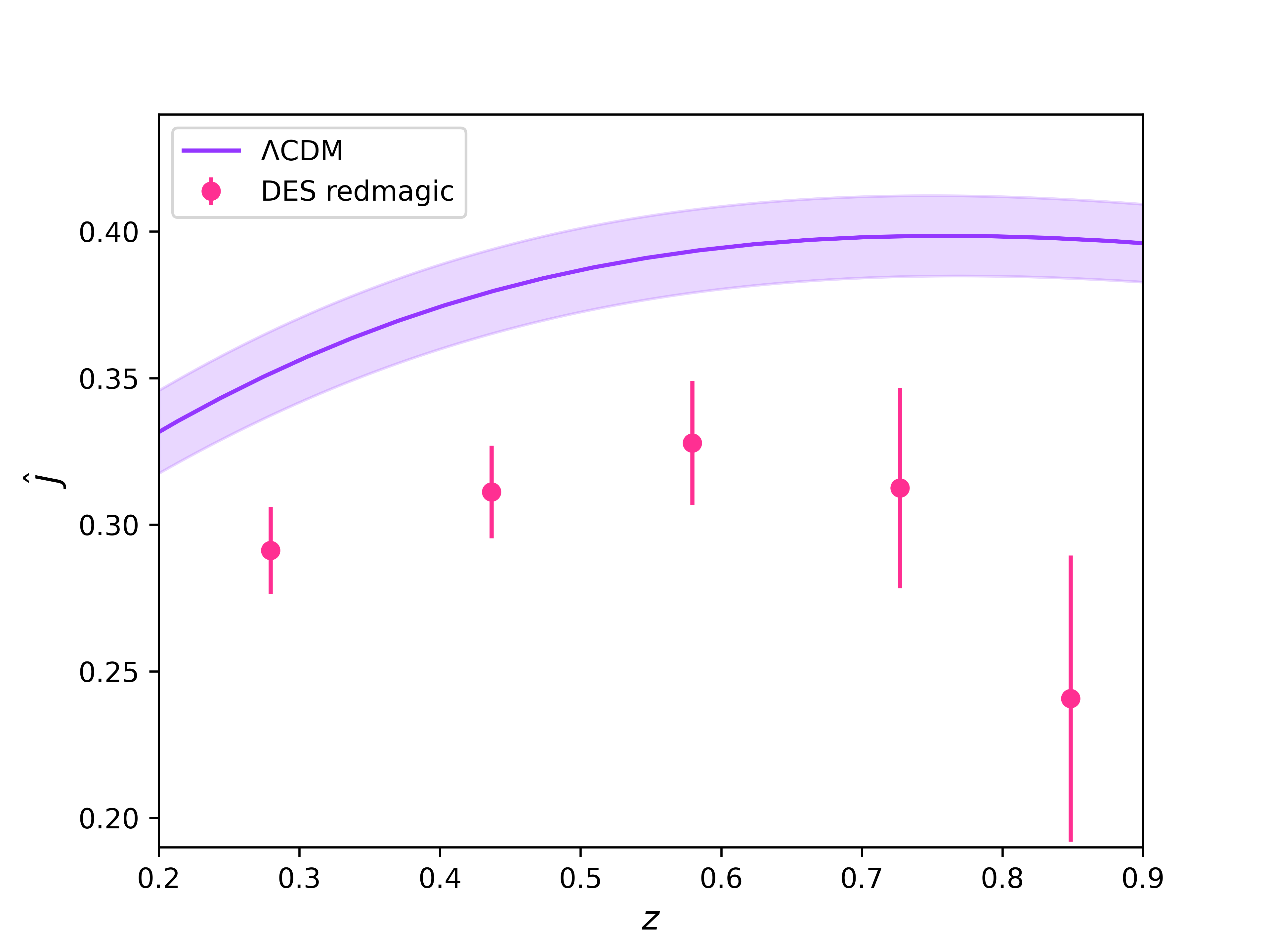
Figure 5: Measured values of $\hat{J}$ at the mean redshifts of the redMaGiC sample, in the baseline analysis, i.e. using priors from Planck on early time cosmological parameters and standard scale cuts. The purple solid line shows the prediction for $\hat{J}$ in $\Lambda$CDM. The shaded regions indicate the 1$\sigma$ uncertainty on this prediction due to uncertainties in the primordial cosmological parameters.

In Fig. 5, we show the measurements of $\hat{J}$ in the five redshift bins of the redMaGiC lens sample: $z\in[0.280,0.437,0.580,0.727,0.849]$, for our baseline analysis, i.e. using Planck priors and standard scale cuts. We also show the $\Lambda$CDM predictions using the cosmological parameters from our analysis. The measurements are systematically below the predictions. The values and 1$\sigma$ error-bars are listed in Table 4.

Table 4: Mean values and 1$\sigma$ error bars for $\hat{J}(z_{i})$ from the redMaGiC sample, in the baseline analysis.

$\hat{J}(z_{1})$	$0.291\pm 0.015$
$\hat{J}(z_{2})$	$0.311\pm 0.016$
$\hat{J}(z_{3})$	$0.328\pm 0.021$
$\hat{J}(z_{4})$	$0.313\pm 0.034$
$\hat{J}(z_{5})$	$0.241\pm 0.049$

Appendix C Additional plots

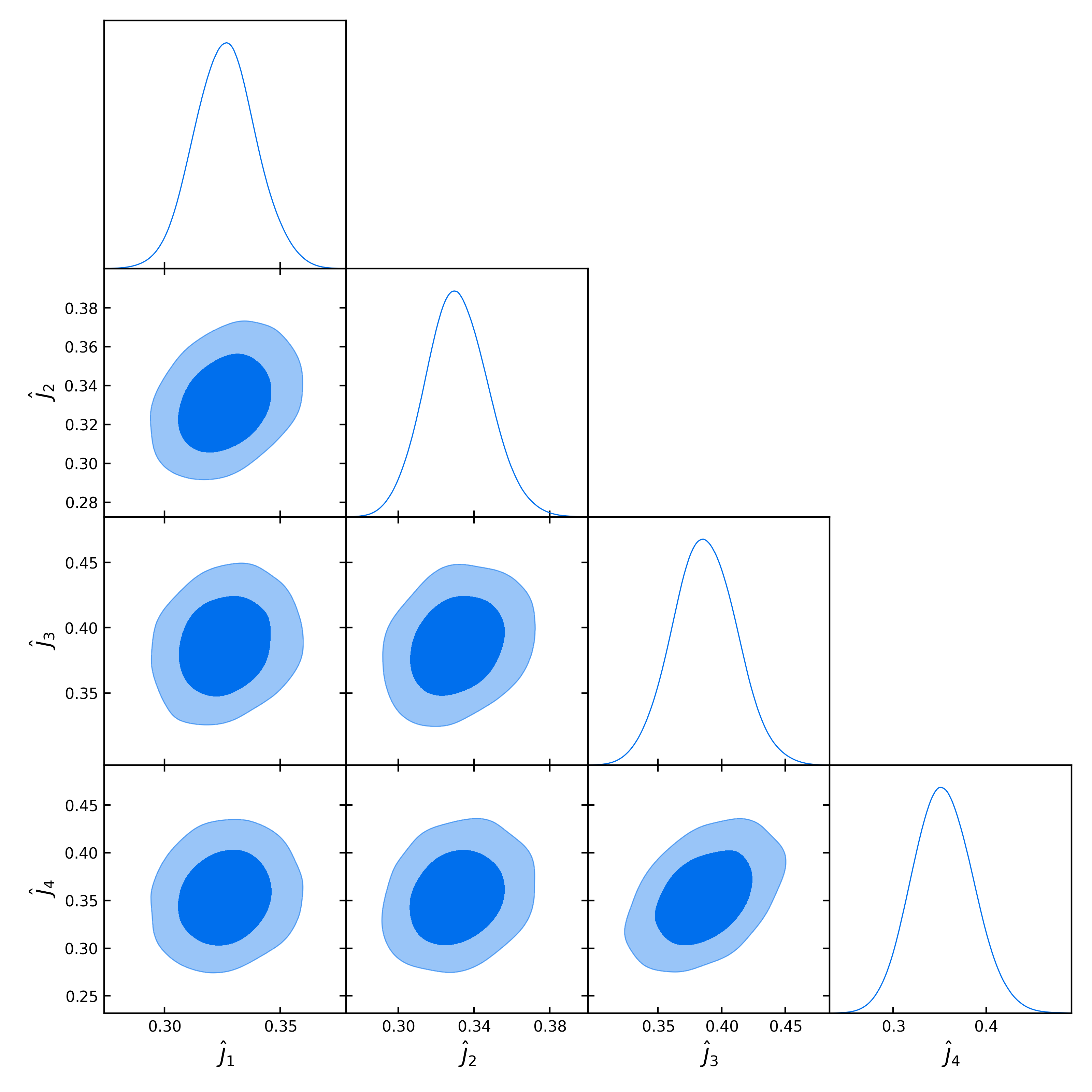
Figure 6: Joint contours for the four values of $\hat{J}$ in the baseline scenario with Planck priors and standard scale cuts.

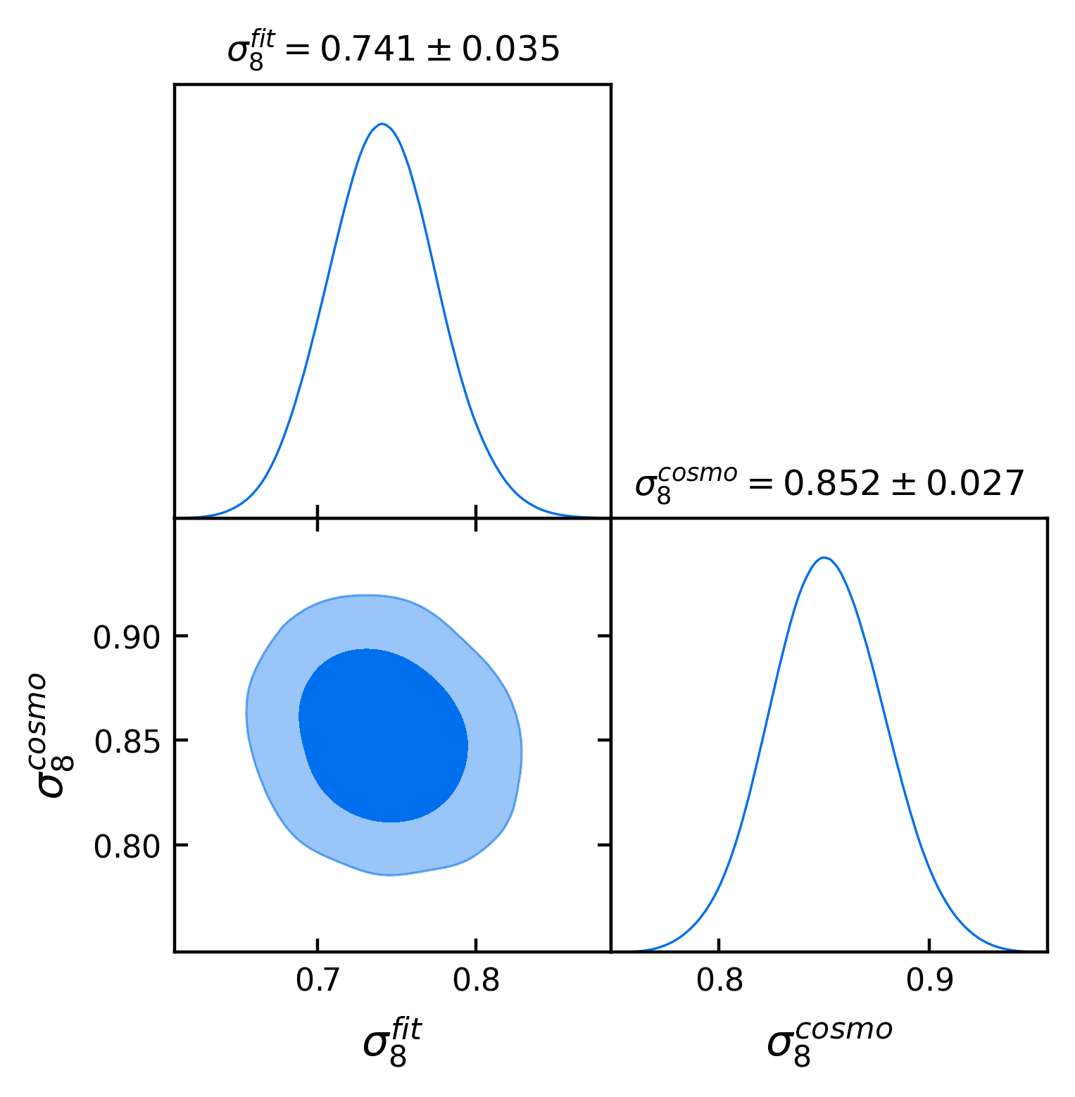
Figure 7: Joint contours for $\sigma^{\rm fit}_{8}(z=0)$ obtained from $\hat{J}$, and $\sigma_{8}^{\rm cosmo}(z=0)$ obtained from cosmological parameters, in the baseline scenario with Planck priors and standard scale cuts.

Figure 8: Joint contours for $\hat{J}$ and the shift $\Delta z_{l}$ and stretch $\sigma z_{l}$ of the photometric distribution in the second bin of the MagLim sample, where the tension is the largest. Here, we show the case without Planck prior and with standard scale cuts.

Here, we show various joint distributions of parameters discussed in the main text. In Fig. 6, we plot the joint contours for $\hat{J}$, showing that the posteriors are close to Gaussian and that there is a mild correlation between the different redshift bins. In Fig. 7, we show the joint distribution of $\sigma_{8}(z=0)$ obtained from $\hat{J}$ and obtained from the cosmological parameters. Finally, in Fig. 8 we show the joint distributions, in the second redshift bin, of $\hat{J}$ and the two nuisance parameters $\Delta z_{l}$ (shift) and $\sigma z_{l}$ (width) that govern the photometric redshift distribution of the lenses.

References

- (1) Supernova Search Team, A. G. Riess, A. V. Filippenko, P. Challis, A. Clocchiatti, A. Diercks et al., Observational evidence from supernovae for an accelerating universe and a cosmological constant, Astron. J. 116 (1998) 1009, arXiv:astro-ph/9805201
- (2) Supernova Cosmology Project, S. Perlmutter et al., Measurements of and from 42 high redshift supernovae, Astrophys. J. 517 (1999) 565, arXiv:astro-ph/9812133
- (3) G. W. Horndeski, Second-order scalar-tensor field equations in a four-dimensional space, International Journal of Theoretical Physics 10 (1974) 363
- (4) J. Noller and A. Nicola, Cosmological parameter constraints for Horndeski scalar-tensor gravity, Phys. Rev. D 99 (2019) 103502, arXiv:1811.12928
- (5) K. Koyama, Cosmological Tests of Modified Gravity, Rept. Prog. Phys. 79 (2016) 046902, arXiv:1504.04623
- (6) DES collaboration, T. M. C. Abbott, M. Aguena, A. Alarcon, O. Alves, A. Amon et al., Dark Energy Survey Year 3 Results: Constraints on extensions to CDM with weak lensing and galaxy clustering, Phys. Rev. D107 (2023) 083504, arXiv:2207.05766
- (7) C. Bonvin and L. Pogosian, Modified Einstein versus Modified Euler for Dark Matter, Nature Astron. 7 (2023) 1127, arXiv:2209.03614
- (8) S. Castello, N. Grimm, and C. Bonvin, Rescuing constraints on modified gravity using gravitational redshift in large-scale structure, Phys. Rev. D106 (2022) 083511, arXiv:2204.11507
- (9) Y.-S. Song and W. J. Percival, Reconstructing the history of structure formation using Redshift Distortions, JCAP 10 (2009) 004, arXiv:0807.0810
- (10) C. Blake, S. Brough, M. Colless, C. Contreras, W. Couch et al., The WiggleZ dark energy survey: the growth rate of cosmic structure since redshift z=0.9, Mon. Not. Roy. Astron. Soc. 415 (2011) 2876, arXiv:1104.2948
- (11) eBOSS collaboration, S. Alam, M. Aubert, S. Avila, C. Balland, J. E. Bautista et al., Completed SDSS-IV extended Baryon Oscillation Spectroscopic Survey: Cosmological implications from two decades of spectroscopic surveys at the Apache Point Observatory, Phys. Rev. D103 (2021) 083533, arXiv:2007.08991
- (12) I. Tutusaus, D. Sobral-Blanco, and C. Bonvin, Combining gravitational lensing and gravitational redshift to measure the anisotropic stress with future galaxy surveys, Phys. Rev. D107 (2023) , arXiv:2209.08987
- (13) Planck, N. Aghanim, Y. Akrami, M. Ashdown, J. Aumont, C. Baccigalupi et al., Planck 2018 results. VI. Cosmological parameters, Astron. Astrophys. 641 (2020) A6, arXiv:1807.06209, [Erratum: Astron. Astrophys. 652, C4 (2021)]
- (14) L. Amendola, M. Kunz, M. Motta, I. D. Saltas, and I. Sawicki, Observables and unobservables in dark energy cosmologies, Phys. Rev. D87 (2013) 023501, arXiv:1210.0439
- (15) L. Amendola, S. Fogli, A. Guarnizo, M. Kunz, and A. Vollmer, Model-independent constraints on the cosmological anisotropic stress, Phys. Rev. D89 (2014) 063538, arXiv:1311.4765
- (16) Euclid, A. Blanchard, S. Camera, C. Carbone, V. F. Cardone, S. Casas et al., Euclid preparation: VII. Forecast validation for Euclid cosmological probes, Astron. Astrophys. 642 (2020) A191, arXiv:1910.09273
- (17) J. Gleyzes, D. Langlois, M. Mancarella, and F. Vernizzi, Effective Theory of Dark Energy at Redshift Survey Scales, JCAP 02 (2016) 056, arXiv:1509.02191
- (18) M. Raveri, L. Pogosian, K. Koyama, M. Martinelli, A. Silvestri et al., Principal reconstructed modes of dark energy and gravity, JCAP 02 (2023) 061, arXiv:2107.12990
- (19) DES, A. Porredon et al., Dark Energy Survey Year 3 results: Cosmological constraints from galaxy clustering and galaxy-galaxy lensing using the MagLim lens sample, Phys. Rev. D 106 (2022) 103530, arXiv:2105.13546
- (20) X. Fang, E. Krause, T. Eifler, and N. MacCrann, Beyond Limber: Efficient computation of angular power spectra for galaxy clustering and weak lensing, JCAP 05 (2020) 010, arXiv:1911.11947
- (21) DES collaboration, T. M. C. Abbott, M. Aguena, A. Alarcon, S. Allam, O. Alves et al., Dark Energy Survey Year 3 results: Cosmological constraints from galaxy clustering and weak lensing, Phys. Rev. D105 (2022) 023520, arXiv:2105.13549
- (22) J. Zuntz, M. Paterno, E. Jennings, D. Rudd, A. Manzotti et al., CosmoSIS: modular cosmological parameter estimation, Astron. Comput. 12 (2015) 45, arXiv:1409.3409
- (23) J. Blazek, N. MacCrann, M. A. Troxel, and X. Fang, Beyond linear galaxy alignments, Phys. Rev. D 100 (2019) 103506, arXiv:1708.09247
- (24) S. Bridle and L. King, Dark energy constraints from cosmic shear power spectra: impact of intrinsic alignments on photometric redshift requirements, New J. Phys. 9 (2007) 444, arXiv:0705.0166
- (25) W. J. Handley, M. P. Hobson, and A. N. Lasenby, PolyChord: nested sampling for cosmology, Mon. Not. Roy. Astron. Soc. 450 (2015) L61, arXiv:1502.01856
- (26) F. Feroz, M. P. Hobson, and M. Bridges, MultiNest: an efficient and robust Bayesian inference tool for cosmology and particle physics, Mon. Not. Roy. Astron. Soc. 398 (2009) 1601, arXiv:0809.3437
- (27) A. Lewis, GetDist: a Python package for analysing Monte Carlo samples, arXiv:1910.13970
- (28) DES, R. Cawthon et al., Dark Energy Survey Year 3 results: calibration of lens sample redshift distributions using clustering redshifts with BOSS/eBOSS, Mon. Not. Roy. Astron. Soc. 513 (2022) 5517, arXiv:2012.12826
- (29) DES, S. Pandey et al., Dark Energy Survey year 3 results: Constraints on cosmological parameters and galaxy-bias models from galaxy clustering and galaxy-galaxy lensing using the redMaGiC sample, Phys. Rev. D 106 (2022) 043520, arXiv:2105.13545
- (30) A. Lewis, A. Challinor, and A. Lasenby, Efficient computation of CMB anisotropies in closed FRW models, Astrophys. J. 538 (2000) 473, arXiv:astro-ph/9911177
- (31) E. Bellini and I. Sawicki, Maximal freedom at minimum cost: linear large-scale structure in general modifications of gravity, JCAP 07 (2014) 050, arXiv:1404.3713
- (32) S. Castello, M. Mancarella, N. Grimm, D. S. Blanco, I. Tutusaus et al., Gravitational Redshift Constraints on the Effective Theory of Interacting Dark Energy, arXiv:2311.14425
- (33) J. Gleyzes, D. Langlois, M. Mancarella, and F. Vernizzi, Effective Theory of Interacting Dark Energy, JCAP 08 (2015) 054, arXiv:1504.05481
- (34) C. Brans and R. H. Dicke, Mach’s principle and a relativistic theory of gravitation, Phys. Rev. 124 (1961) 925
- (35) I. Sawicki, I. D. Saltas, L. Amendola, and M. Kunz, Consistent perturbations in an imperfect fluid, JCAP 01 (2013) 004, arXiv:1208.4855
- (36) S. M. Carroll, V. Duvvuri, M. Trodden, and M. S. Turner, Is cosmic speed - up due to new gravitational physics?, Phys. Rev. D 70 (2004) 043528, arXiv:astro-ph/0306438
- (37) Y.-S. Song, W. Hu, and I. Sawicki, The Large Scale Structure of f(R) Gravity, Phys. Rev. D 75 (2007) 044004, arXiv:astro-ph/0610532
- (38) S. M. Carroll, I. Sawicki, A. Silvestri, and M. Trodden, Modified-Source Gravity and Cosmological Structure Formation, New J. Phys. 8 (2006) 323, arXiv:astro-ph/0607458
- (39) D. N. Vollick, 1/R Curvature corrections as the source of the cosmological acceleration, Phys. Rev. D 68 (2003) 063510, arXiv:astro-ph/0306630
- (40) Kilo-Degree Survey, Dark Energy Survey, T. M. C. Abbott et al., DES Y3 + KiDS-1000: Consistent cosmology combining cosmic shear surveys, Open J. Astrophys. 6 (2023) 2305.17173, arXiv:2305.17173