Effects of coordination and stiffness scale-separation in disordered elastic networks

Abstract

Many fibrous materials are modeled as elastic networks featuring a substantial separation between the stiffness scales that characterize different microscopic deformation modes of the network’s constituents. This scale separation has been shown to give rise to emergent complexity in these systems’ linear and nonlinear mechanical response. Here we study numerically a simple model featuring said stiffness scale-separation in two-dimensions and show that its mechanical response is governed by the competition between the characteristic stiffness of collective nonphononic soft modes of the stiff subsystem, and the characteristic stiffness of the soft interactions. We present and rationalize the behavior of the shear modulus of our complex networks across the unjamming transition at which the stiff subsystem alone loses its macroscopic mechanical rigidity. We further establish a relation in the soft-interaction-dominated regime between the shear modulus, the characteristic frequency of nonphononic vibrational modes, and the mesoscopic correlation length that marks the crossover between a disorder-dominated response to local mechanical perturbations in the near-field, and a linear, continuum-like response in the far field. The effects of spatial dimension on the observed scaling behavior are discussed, in addition to the interplay between stiffness scales in strain-stiffened networks, which are relevant to the nonlinear mechanics of non-Brownian biopolymer networks.

I Introduction

Disordered networks of unit masses connected by Hookean springs constitute a popular minimal model for studying the elasticity of disordered solids [1, 2, 3, 4, 5, 6, 7, 8, 9]. In this simple model the key parameter that controls macro- and microscopic elasticity is the mean node coordination $z$. Several scaling laws have been established for characteristic length-scales [10, 11, 9], frequency-scales [2, 5, 7], elastic moduli [2, 4] and their fluctuations [12, 13] in terms of the difference $\delta z\!\equiv\!z\!-\!z_{\rm c}$, where $z_{\rm c}\!\equiv\!2{\,\mathchar 22\relax\mkern-12.0mud}$ is the Maxwell threshold, and ${\,\mathchar 22\relax\mkern-12.0mud}$ stands for the dimension of space.

Inspired by observations from rheological experiments on biomaterials [14, 15], the simple disordered spring-network model in two dimensions (2D) was supplemented by bending (angular) interactions that penalize changes in the angles formed between edges connected to the same node [16, 6, 17, 18]. Particularly relevant to investigating fibrous biomaterials is the case in which the stiffness associated with these angular interactions is far smaller than the stiffness associated with the stretching or compression of the radial, Hookean springs. In this limit, the phenomenon of strain-stiffening of athermal, floppy ($z\!<\!z_{\rm c}$) elastic networks stabilized by soft angular interactions was thoroughly investigated in recent years [19, 20, 21, 22, 23, 24, 18, 25, 26]. Despite the aforementioned efforts and progress, the combined effects of changing both coordination $z$ and the ratio $\kappa$ of bending-to-stretching stiffnesses of disordered elastic networks, have not been fully resolved.

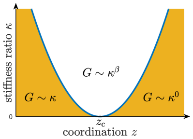
Figure 1: Scaling regimes of the shear modulus $G$ in disordered networks characterized by their coordination $z$ and the bending-to-stretching stiffness ratio $\kappa$. The crossover between the small- and large-$\kappa$ scaling occurs when $\kappa\!\sim\!(z\!-\!z_{\rm c})^{2}$, see text for discussion. We find $\beta\!=\!0.55$ in two-dimensions, and $\beta\!=\!0.5$ in three-dimensions.

In this work we fill this gap and study the mechanics of disordered spring networks endowed with soft, angular interactions, under variations of both the coordination $z$ of the underlying stiff network, and of the ratio $\kappa\!\ll\!1$ of bending-to-stretching stiffness. We trace out the crossover in our networks’ shear modulus between a regime dominated by the stiff subnetwork’s nonphononic soft (for $z\!>\!z_{\rm c}$) or zero (for $z\!<\!z_{\rm c}$) modes, and a regime dominated by the soft angular interactions, as illustrated in Fig. 1. Interestingly, we find that, in both regimes, the shear modulus $G$ scales (approximately in 2D and exactly in 3D) with the characteristic frequency of soft, nonphononic modes, independent of whether the latter are dominated by the stiff subnetwork, or by the soft angular interactions, in states for which the stiff subnetwork alone has a finite shear modulus. In addition, we show that the same scaling argument made in Ref. [27] for the mesoscopic correlation length $\xi$ — that marks the crossover between a non-affine, near-field disorder-dominated response to local perturbations, to an affine, far-field linear-continuum-elastic-like response —, holds in the unexplored, angular-interaction-dominated regime. We further point out a slight but measurable and consistent difference between scaling exponents measured for shear moduli in 2D compared to 3D. Finally, we investigate the effects of stiffness scale separation in strain-stiffened networks in 2D.

This work is structured as follows; in Sect. II we present the models and methods employed, and the precise definitions of the key observables considered in this work. In Sect. III we present our numerical results for the elastic properties of isotropic disordered networks and rationalize them using scaling arguments and building on existing arguments and results. In Sect. IV we show results and discuss the scaling behavior seen for strain-stiffened elastic networks. We summarize this work and discuss future research questions in Sect. V.

II Numerical model, methods and observables

We employ a well-studied model of athermal biopolymer fibrous materials [16, 6, 17, 18]. Given a disordered, two-dimensional (2D) graph of nodes and edges with some connectivity $z$ (see below how graphs are obtained in this study), we assign a Hookean spring with stiffness $k_{r}$ (set to unity in our calculations) at its rest length $\ell$ on each edge. Every two edges emanating from the same node — with no other edge between them — form angles $\theta$; we assign an angular spring at its rest-angle $\theta^{(0)}$ to each such angle, with stiffness $k_{\theta}$ that has units of energy. The potential energy of this model therefore reads

$$U={\textstyle\frac{1}{2}}k_{r}\!\!\!\!\sum_{\mbox{\scriptsize edges }ij}\!\!\!\!(r_{ij}-\ell_{ij})^{2}+{\textstyle\frac{1}{2}}k_{\theta}\!\!\!\!\!\sum_{\mbox{\scriptsize angles }ijk}\!\!\!\!\!(\theta_{ijk}-\theta^{(0)}_{ijk})^{2}\,.$$ (1)

In what follows we express all energies in terms of $k_{r}\bar{\ell}^{2}$ and elastic moduli in terms of $k_{r}\bar{\ell}^{2-{\,\mathchar 22\relax\mkern-12.0mud}}$ where $\bar{\ell}\!\equiv\!(V/N)^{1/{\,\mathchar 22\relax\mkern-12.0mud}}$ with $V$ denoting the system’s volume, $N$ denoting the number of nodes, and ${\,\mathchar 22\relax\mkern-12.0mud}$ stands for the dimension of space. Lengths are expressed in terms of $\bar{\ell}$. Importantly, we define the ratio of bending to stretching stiffnesses as $\kappa\!\equiv\!k_{\theta}/k_{r}\bar{\ell}^{2}$. For all calculations presented in what follows, we average the observables over about 100 independently created configurations. In what follows, the number of nodes $N$ employed in our networks is stated in the introduction of each data set.

Our initial graphs were obtained by adopting the contact network of highly compressed soft-disc packings. To obtain networks at a target coordination $z$, we dilute the edges following the algorithm described in Ref. [28]; this algorithm produces networks with small node-to-node coordination fluctuations, and by such avoids the creation of locally rigid clusters [29, 30]. An example of a network generated with this algorithm, at $z\!=\!z_{\rm c}$, is shown in Fig. 2.

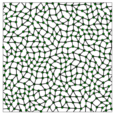
Figure 2: An example of an isostatic (i.e. featuring $z\!=\!z_{\rm c}$), packing-derived network used in this study. Edges are diluted to reach the target coordination using the algorithm described in Ref. [28], see text for discussion.

We also carried out calculations in a three-dimensional complex elastic network model. In this model the disordered network considered are also derived from contact-networks of soft-sphere packings; however, in order to dilute the edges to reach some target coordination $z$, we employ the algorithm described in Ref. [31], which — similarly to the algorithm employed for our 2D networks — suppresses large node-to-node coordination fluctuations. In our 3D model we do not consider soft angular interactions; instead, for the sake of simplicity we follow Refs. [3, 23] and connect soft springs of stiffness $\kappa k_{r}$ to all nearby nodes — at distance $r\!\leq\!1.1\bar{\ell}$ apart — that are not connected by a stiff (i.e. of stiffness $k_{r}$) spring, and recall that $\kappa\!\ll\!1$. For this system, the coordination $z$ reported pertains to the stiff subnetwork. As we will show below, and as also demonstrated in [23], these soft interactions give rise to the same scaling behavior as seen for our 2D networks with soft angular interactions.

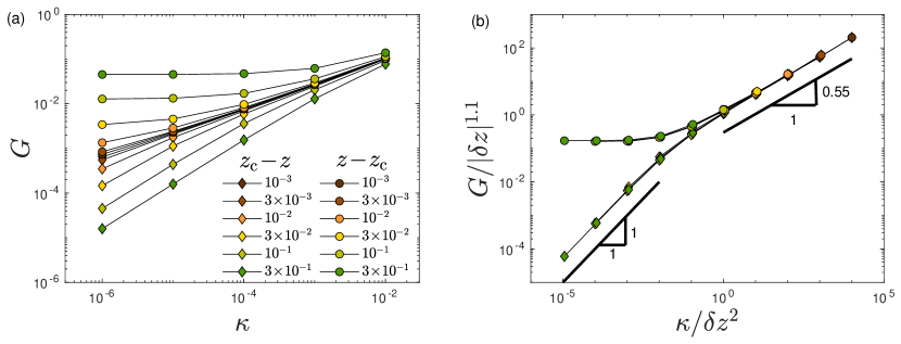
Figure 3: (a) The shear modulus $G$ of 2D isotropic, disordered elastic networks with $N\!=\!102400$ nodes, for various coordinations $z$ (see legend, and recall that $z_{\rm c}\!\equiv\!2{\,\mathchar 22\relax\mkern-12.0mud}$ with ${\,\mathchar 22\relax\mkern-12.0mud}$ denoting the spatial dimension), plotted against the stiffness ratio $\kappa$. (b) Same data as panel (a), plotted while rescaling the axes as described by the axes labels, see text for discussion.

We also investigated the behavior of strain-stiffened networks in 2D; to this aim, we employed the following two-step procedure [26]: isotropic floppy networks with $z\!<\!z_{\rm c}$ were sheared — using the standard athermal, quasistatic scheme [32] — while setting $\kappa\!=\!0$, until the ratio of the typical net-force on nodes to the typical compressive/tensile spring forces first drops below $10^{-8}$. The shear strain $\gamma_{\rm c}$ at which this happens is resolved up to strain increments of $10^{-6}$. Then, we gradually introduce angular interactions of dimensionless stiffness $\kappa$ – in the form of the 2nd term of Eq. (1) above. Once the soft interactions are introduced, the system is returned to a mechanically stable state by means of a potential energy minimization [33]. Importantly, in this step the rest-angles considered are those defined in the isotropic, undeformed network. This two-step procedure allows us to accurately determine the critical stiffening strain $\gamma_{\rm c}$, which is important since observables such as the shear modulus vary rapidly with strain at small $\kappa$ near $\gamma_{\rm c}$ [26].

We conclude this Section with precise definitions of the key observables considered in this work. In Appendix A we provide easily implementable microscopic expressions for the angular potential and its derivatives with respect to coordinates and simple-shear-strain.

Our prime focus in this work is on the athermal shear modulus, defined as

$$G=\frac{1}{V}\bigg{(}\frac{\partial^{2}U}{\partial\gamma^{2}}-\frac{\partial^{2}U}{\partial\gamma\partial\mathitbf x}\cdot\mbox{\boldmath${\cal H}$}^{-1}\cdot\frac{\partial^{2}U}{\partial\gamma\partial\mathitbf x}\bigg{)}\,,$$ (2)

where $V\!=\!L^{\,\mathchar 22\relax\mkern-12.0mud}$ is the system’s volume, $U$ is the potential energy, $\gamma$ is a simple shear strain parameter, $\mathitbf x$ denotes the nodes’ coordinates, and $\mbox{\boldmath${\cal H}$}\!\equiv\!\frac{\partial^{2}U}{\partial\mathitbf x\partial\mathitbf x}$ is the Hessian matrix. The shear modulus characterizes the macroscopic elastic response of the material; a microscopic characterization of the material’s response is encoded in the typical nonaffine displacements squared, defined as

$$u_{\mbox{\scriptsize na}}^{2}\equiv\frac{\mathitbf u_{\mbox{\scriptsize na}}\cdot\mathitbf u_{\mbox{\scriptsize na}}}{N}=\frac{\frac{\partial^{2}U}{\partial\gamma\partial\mathitbf x}\cdot\mbox{\boldmath${\cal H}$}^{-2}\cdot\frac{\partial^{2}U}{\partial\gamma\partial\mathitbf x}}{N}\,.$$ (3)

Finally, we study the spatial properties of the typical displacement response $\mathitbf u_{d}$ to local force dipoles [10, 9, 31], defined as

$$\mathitbf u_{d}=\mbox{\boldmath${\cal H}$}^{-1}\cdot\mathitbf d\,,$$ (4)

where $\mathitbf d\!\equiv\!\frac{\partial r}{\partial\mathitbf x}$ is a unit force dipole applied to a radial spring with length $r$.

III Elasticity of Isotropic disordered networks

III.1 Shear modulus of isotropic networks

In Fig. 3a we present our results concerning the shear modulus $G(z,\kappa)$ and its dependence on coordination $z$ and the stiffness ratio $\kappa$ in our isotropic (undeformed) 2D disordered networks prepared as explained in Sect. II. Here we employed networks of $N\!=\!102400$ nodes at various coordinations $z$ as displayed in the figure legend. In Fig. 3b we show the same data rescaled by $\delta z^{\beta}$ with $\beta\!=\!1.1$, and plotted against the rescaled stiffness ratio $\kappa/\delta z^{2}$, to find a convincing data collapse. Our data suggest the scaling form

$$G(z,\kappa)=|\delta z|^{\beta}{\cal F}_{\pm}(\kappa/\delta z^{2})\,,$$ (5)

where ${\cal F}_{\pm}(y)$ stands for a pair of scaling functions corresponding to $\delta z\!\gtrless\!0$, with the following properties

$$\begin{matrix}{\cal F}_{+}(y)\sim&\mbox{const}\,,&y\ll 1\,,\\ {\cal F}_{-}(y)\sim&y\,,&y\ll 1\,,\\ {\cal F}_{\pm}(y)\sim&y^{\beta/2}\,,&y\gg 1\,.\end{matrix}$$ (6)

A convincing collapse is obtained by setting $\beta\!=\!1.1$ in the scaling analysis of Fig. 3.

We next rationalize the observed scaling behavior using scaling argument and building on previously established results.

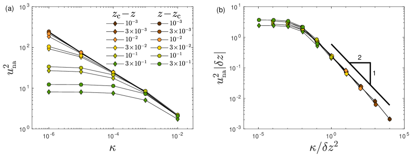
Figure 4: (a) The typical magnitude squared of nonaffine displacements (see Eq. (3) for precise definition), calculated for 2D isotropic disordered networks at various coordinations $z$ as specified by the figure legend, and plotted against the stiffness ratio $\kappa$ (b) Same data as panel (a), but cast into a scaling form, see text for details and discussion.

III.1.1 $G$ in the hypostatic regime $z\!<\!z_{\rm c}$

It is known that for hypostatic ($z\!<\!z_{\rm c}$), isotropic, disordered spring networks in the absence of bending interactions, namely $\kappa\!=\!0$, the shear modulus is identically zero. In the limit $\kappa\!\to\!0$ the only (dimensionless) stiffness scale is $\kappa$, and therefore $G\!\sim\!\kappa$ in the $\kappa\!\to\!0$ limit, as indeed shown in previous work [6, 22, 34, 21, 18]. The same conclusion can be obtain with more rigor following the framework of Ref. [23], where the $\kappa\!\to\!0^{+}$ limit is considered, reducing the problem to a geometric one. In the same work and also earlier in Ref. [3] it was shown and rationalized that $G\!\sim\!1/\delta z$ for hypostatic elastic networks stabilized by weak interactions. Therefore, in the small-$\kappa$ limit, we expect that $G\!\sim\!\kappa/\delta z$. In Fig. 3 we show that as $\kappa\!\to\!0$, $G\!\sim\!\kappa/\delta z^{2-\beta}$, where the scaling exponent $2\!-\!\beta\!\approx 0.9$ is close to the prediction.

What would happen at larger $\kappa$? Since $\kappa$ is a stiffness scale, it is reasonable to compare it to the square of the characteristic frequency $\omega_{\star}\!\sim\!\delta z$ [2, 35, 5, 7, 36] of the stiff subnetwork. We would therefore expect that once $\kappa$ is of order $\delta z^{2}$, the scaling behavior of $G$ should change. In other words, we expect that $\kappa/\omega_{\star}^{2}\!\sim\!\kappa/\delta z^{2}$ should form the relevant scaling variable, as indeed seen in Fig. 3b and in the rest of the datasets presented in this work.

III.1.2 $G$ in the hyperstatic regime $z\!>\!z_{\rm c}$

Since $\omega_{\star}\!\sim\!|\delta z|$ both above and below the isostatic point $z_{\rm c}$ [2, 7], the same argument for the relevant scaling variable $\kappa/\delta z^{2}$ should hold in the hyperstatic regime $z\!>\!z_{\rm c}$, as indeed observed in Fig. 3b. In addition, in the limit $\kappa\!\ll\!\delta z^{2}$ we expect the known behavior $G\!\sim\!\delta z^{\beta}$ to prevail, i.e. $G$ should become independent of $\kappa$, as indeed observed in Fig. 3.

III.1.3 $G$ in the critical regime $\kappa\!>\!\delta z^{2}$

Interestingly, in the critical regime we find ${\cal F}_{\pm}(y)\!\sim\!y^{\beta/2}$ (for $y\!\gg\!1$). How can this scaling be rationalized? We expect that in the $\kappa\!\gg\!\delta z^{2}$ regime the stiff subnetwork’s floppy modes, of frequency $\omega_{\star}\!\sim\!\delta z$ are stiffened by the angular interactions to feature frequencies of order $\sqrt{\kappa}$. We thus expect the characteristic frequency $\varpi$ of soft, nonphononic modes to follow

$$\varpi\sim\left\{\begin{matrix}\omega_{\star}\sim|\delta z|&\mbox{for}&\kappa\ll\delta z\\ \sqrt{\kappa}&\mbox{for}&\kappa\gg\delta z^{2}\end{matrix}\right.$$ (7)

Since the general relation between the shear modulus $G$ and the frequency of soft, nonphononic modes is theoretically predicted to follow $G\!\sim\!\omega_{\star}$ for $z\!>\!z_{\rm c}$ and in the absence of bending interactions, one could expect that, also in the critical $\kappa\!\gg\!\delta z^{2}$ regime, we would find $G\!\sim\!\varpi\!\sim\!\sqrt{\kappa}$. In practice, we rather find $G\!\sim\!\kappa^{\beta/2}$ with $\beta\!=\!1.1$ (cf. Fig. 3b), i.e. $G\!\sim\!\kappa^{0.55}$ - very close to the scaling suggested above. In Sect. III.4 below we show that the deviation from the expected scaling $G\!\sim\!\sqrt{\kappa}$ appears to be a 2D effect.

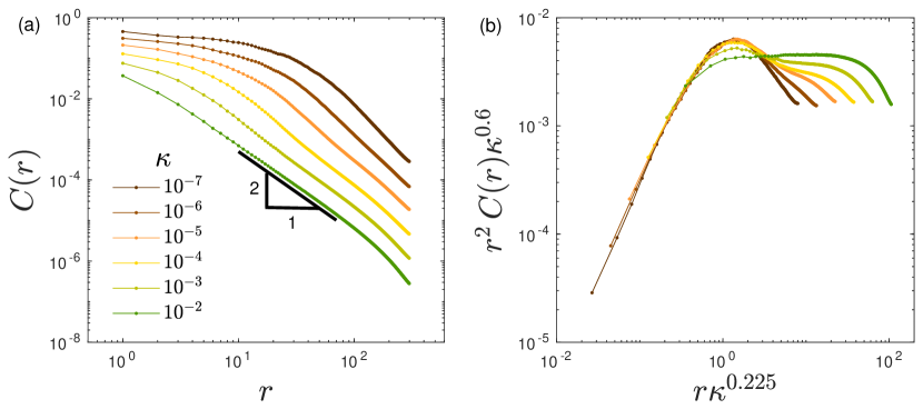
Figure 5: (a) Spatial decay of the displacement response functions $C(r)$ to local force dipoles, see text for definition. (b) Rescaling the axes allows to extract the $\kappa$-dependence of the length $\xi$ that marks the crossover between a nonaffine, disorder-dominated near field, and an affine, continuum-linear-elastic-like response in the far field, see text for further details and discussion.

III.2 Nonaffine displacements of isotropic networks

We next turn to studying the typical nonaffine displacements squared $u_{\mbox{\scriptsize na}}^{2}$ (see Eq. (3) above for a precise definition) in our 2D networks as a function of the coordination $z$ and the stiffness ratio $\kappa$. Fig. 4 displays our results; in panel (a) we show the raw data, while panel (b) presents a scaling collapse, where, similarly to the analysis and argumentation provided above for the shear modulus, we consider the scaling variable $\kappa/\delta z^{2}$ to control the behavior of $u_{\mbox{\scriptsize na}}^{2}$ for various $\kappa$ and $z$. Different from the shear modulus analysis, here the $y$-axis is factored by $|\delta z|$, rationalized next for the different scaling regimes.

III.2.1 $u_{\rm na}^{2}$ outside of the critical regime $\kappa\!\ll\!\delta z^{2}$

In Ref. [3] it was argued and demonstrated that $u_{\mbox{\scriptsize na}}^{2}\!\sim\!1/\delta z$ in the hypostatic $z\!<\!z_{\rm c}$ regime, while in Ref. [37] the same was argued and demonstrated for the hyperstatic $z\!>\!z_{\rm c}$ regime. Furthermore, a dimensional analysis of the $\kappa\!\to\!0$ expression for $\mathitbf u_{\mbox{\scriptsize na}}$ of Ref. [23] (see Eq. (16) therein) implies that $u_{\mbox{\scriptsize na}}^{2}$ becomes independent of $\kappa$ in the $\kappa\!\to\!0$ limit. We therefore expect that $u_{\mbox{\scriptsize na}}^{2}\!\sim\!1/\delta z$ for all $z,\kappa$, as indeed validated by the scaling collapse of Fig. 4b.

III.2.2 $u_{\rm na}^{2}$ in the critical regime $\kappa\!\gg\!\delta z^{2}$

Let us repeat the same line of argumentation as invoked for the scaling of the shear modulus in the critical regime $\kappa\!\gg\!\delta z^{2}$; in the absence of any angular interactions, namely on the $\kappa\!=\!0$ line, one finds $u_{\mbox{\scriptsize na}}^{2}\!\sim\!1/\delta z\!\sim\!1/\omega_{\star}$. Generalizing this result to a situation where nonphononic modes are stiffened by angular interactions — such that $\varpi\!\sim\!\sqrt{\kappa}$ (cf. Eq. (7) above) —, one may then expect $u_{\mbox{\scriptsize na}}^{2}\!\sim\!1/\varpi\!\sim\!1/\sqrt{\kappa}$ for $\kappa\!\gg\!\delta z^{2}$. In Fig. 4 this expectation is validated by our numerical simulations, to find very good agreement.

III.3 The crossover length $\xi$ of isotropic networks

In the absence of bending interactions (i.e. setting $\kappa\!=\!0$), disordered elastic networks feature a correlation length $\xi\!\sim\!1/\sqrt{\delta z}$ that marks the crossover between a near-field, nonaffine, disorder-dominated response to local force perturbations, to a far-field, affine, continuum-linear-elastic-like response, as shown in several prior works [38, 10, 31]. Here we probe the $\kappa$-dependence of this correlation length in 2D networks of $N\!=\!409600$ nodes, and at $z\!=\!z_{\rm c}\!=\!4$ such that $\xi\!\sim\!L$ in the absence of angular interactions.

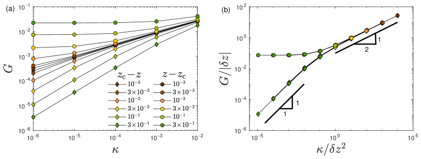
Figure 6: (a) The shear modulus of 3D elastic networks with coordinations various $z$ (see figure legend) — stabilized by additional soft springs of dimensionless stiffness $\kappa\!\ll\!1$ (see text for precise details)—, is plotted against $\kappa$. (b) Same data as panel (a) cast into the predicted scaling form, see text for discussion.

To extract the length $\xi(\kappa)$, we apply a unit dipole force to a single spring to obtain the displacement field $\mathitbf u_{d}$, as described in Eq. (4). We then calculate the average of the displacement response squared — denoted $C(r)$ — over a shell of radius $r$ away from the force dipole. Continuum elasticity predict that the far field should decay as $1/r$ — hence its squared amplitude as $1/r^{2}$ —, as we indeed find for the largest $\kappa$’s probed, cf. Fig. 5a.

How should $\xi$ scale with the stiffness ratio $\kappa$? Here we invoke the scaling argument put forward in Ref. [27]; a continuum, linear-elastic response can be seen if the system is large enough to accommodate elastic waves that are softer than the characteristic frequency of nonphononic modes. This means that a crossover between the nonaffine, disordered response — dominated by nonphononic modes — to an affine, continuum-linear-elastic like response, dominated by elastic waves, occurs when

$$\frac{\sqrt{G}}{\xi}\sim\varpi\,.$$ (8)

For our networks with $z\!=\!z_{\rm c}\!=\!4$ we always satisfy $\kappa\gg\delta z^{2}$ and therefore $\varpi\!\sim\!\sqrt{\kappa}$ (cf. Eq. (7)) and $G\!\sim\!\kappa^{\beta/2}$ with $\beta\!\approx\!1.1$, resulting in the prediction

$$\xi\sim\kappa^{-\frac{2-\beta}{4}}\sim\kappa^{-0.225}\,.$$ (9)

This prediction is nicely validated in Fig. 5b, where the rescaling of both axes leads to an alignment and collapse of the peaks. We emphasize that the exponent $\beta$ was fit in the data-collapse of Fig. 3; here we simply test the resulting predicted exponent $(2\!-\!\beta)/4\!=\!0.225$; we do not claim to have determined it to the third decimal, but rather merely support our scaling argument for $\xi$.

In Sect. III.4 below we show data supporting the theoretical prediction $\beta\!=\!1$ in 3D, which leads us to expect that $\xi\!\sim\!\kappa^{-1/4}$ in 3D, to be validated in future work.

III.4 Elasticity of disordered networks in 3D

In this final Subsection we show that the scaling behavior seen in 2D networks endowed with soft angular interactions is also seen in 3D, using a different, simpler form of soft interactions. In particular, instead of defining angular interactions in 3D, we simply connect nearby nodes — that are not already connected by stiff springs — by soft springs, of stiffness $\kappa k_{r}$, and see Sect. II for further details.

We focus here on the shear modulus $G(\kappa,z)$, similar to the analysis presented for our 2D networks in Fig. 3. The results are displayed in Fig. 6; panel (a) shows the raw data for the shear modulus for a variety of coordinations $z$ and stiffness ratios $\kappa$, while panel (b) employs a rescaling of the axes to find a data collapse. For our 3D networks, are data are consistent with the same scaling form given by Eqs. (5) and (6) but with $\beta\!=\!1$, consistent with theoretical predictions [2, 4, 6]. We conclude that exponents $\beta\!\neq\!1$ appear to be a 2D effect, and that the precise functional form of the soft interactions does not change the scaling behavior observed. We note finally that the exponents obtained from our scaling analysis of 3D networks agree perfectly with Effective Medium Theory calculations in 2D [6, 8].

IV Elasticity of strain-stiffened networks

Strain stiffening refers to the phenomenon in which a hypostatic (floppy) network with soft (but nonzero) angular (bending) interactions — with $\kappa\!\ll\!\delta z^{2}$ — is deformed such that, as some critical strain $\gamma_{\rm c}$ is approached, the shear modulus grows substantially, from $G\!\sim\!\kappa$ (for $\kappa\!\ll\!\delta z^{2}$) in the undeformed, isotropic states, to $G\!\sim\!{\cal O}(1)$ as $\gamma\!\to\!\gamma_{\rm c}$ [39, 40, 24, 26]. Here we study crossover effects between $\kappa\!\ll\!\delta z^{2}$ and $\kappa\!\gg\!\delta z^{2}$ in strain-stiffened networks in 2D, similar to our analysis presented in the previous Section for isotropic, disordered networks.

In order to sharply identify the critical strain $\gamma_{\rm c}$, we employ the following ‘two-step’ procedure [26]: we first set $\kappa\!=\!0$ in our isotropic networks, and employ the athermal, quasistatic deformation scheme in which small strain increments are applied, following each one with a potential-energy minimization [33]. Under $\kappa\!=\!0$ conditions, the shear modulus is identically zero for $\gamma\!<\!\gamma_{\rm c}$, and jumps discontinuously to $G\!\sim\!\delta z$ at $\gamma\!=\!\gamma_{\rm c}$. Details about the detection of $\gamma_{\rm c}$ are provided in Sect. II above.

Once strain-stiffened networks at $\gamma\!=\!\gamma_{\rm c}$ are at hand, we then gradually introduce the soft angular interactions, similarly to the athermal quasistatic deformation scheme: after increasing $\kappa$ to some target value, we restore mechanical equilibrium by a potential energy minimization. We then analyze the elastic properties of these networks as a function of $\kappa$ and $z\!<\!z_{\rm c}$, and we note that, for these calculations we chose $N\!=\!25600$.

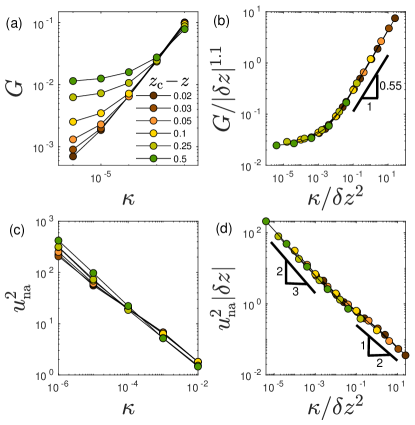
Figure 7: (a) The shear modulus $G$ of 2D hypostatic strain-stiffened networks at various coordinations as indicated by the legend (b) Same data as panel (a), cast into the expected scaling form, see text for details. (c) The characteristic magnitude squared of nonaffine displacements, $u_{\mbox{\scriptsize na}}^{2}$, for the same coordinations as indicated in the legend of panel (a). (d) Scaling collapse of $u_{\mbox{\scriptsize na}}^{2}$ according to the expected form, see text for detailed discussion.

The results are presented in Fig. 7; as expected, the relevant scaling variable is again $\kappa/\delta z^{2}$, just like we have established for isotropic networks above. In panel (a) we show the raw data for the shear modulus $G$ and the typical square of the node-wise nonaffine displacements $u_{\mbox{\scriptsize na}}^{2}$. Despite that here $z\!<\!z_{\rm c}$, the shear modulus data precisely resembles the shear modulus data of isotropic, $z\!>\!z_{\rm c}$ states, cf. Fig. 3a, and follows the exact same scaling form of ${\cal F}_{+}(y)$ (cf. Eq. (5)), namely $G\!\sim\!|\delta z|^{\beta}$ (i.e. independent of $\kappa$, and notice that here $\delta z\!<\!0$) for $\kappa\!\ll\!\delta z^{2}$, and $G\!\sim\!\kappa^{\beta/2}\!\sim\!\kappa^{0.55}$ (independent of $\delta z$) for $\kappa\!\gg\!\delta z^{2}$. These scaling behaviors are validated by the scaling collapse of Fig. 7b.

In Fig. 7b we show data for the typical nonaffine displacements squared $u_{\mbox{\scriptsize na}}^{2}$ of strain-stiffened networks. In the large-$\kappa$ regime, we find the same behavior as seen for isotropic networks, namely that $u_{\mbox{\scriptsize na}}^{2}\!\sim\!1/\sqrt{\kappa}$ (see Fig. 7d), independent of $\delta z$ and consistent with expectations as discussed in Sect. III.2.2 above for isotropic networks. Interestingly, and in contrast with the large-$\kappa$ regime, the scaling behavior of $u_{\mbox{\scriptsize na}}^{2}$ with $\kappa$ is different compared to that seen for isotropic networks in the $\kappa\!\ll\!\delta z^{2}$ regime; in particular, in this regime we find a singular scaling $u_{\mbox{\scriptsize na}}^{2}\!\sim\!\kappa^{-2/3}$ as predicted theoretically in Ref. [26] for strain-stiffened states, and observed in previous simulational work [18, 25] for networks with various geometries. This should be compared to the behavior of $u_{\mbox{\scriptsize na}}^{2}$ in the small-$\kappa$ regime of isotropic states, where it is predicted and observed to become $\kappa$-independent (for any $z$), cf. discussion in Sect. III.2.1.

V summary and discussion

In this work we explored the elastic properties of disordered Hookean spring networks featuring angular interactions whose characteristic stiffness is far smaller than the stiffness associated with the networks’ radial springs. We traced out the different scaling regimes in terms of the coordination $z$ and the ratio $\kappa$ between the angular- and radial-spring-stiffnesses. This was done in 2D both for undeformed, isotropic systems and for strain-stiffened states, the latter is restricted (by construction) to hypostatic ($z\!<\!z_{\rm c}$) systems. In 3D we explored similar questions, but substituted the angular interactions employed in 2D with a simpler form of weak interactions.

We found and rationalized that the scaling variable that controls the elastic properties of these complex networks is the ratio $\kappa/\delta z^{2}$. This ratio expresses the competition between the characteristic stiffness $\sim\!\delta z^{2}$ of nonphononic soft modes of the stiff subnetwork (i.e. in the absence of angular interactions), and the stiffness $\sim\!\kappa$ of angular interactions.

Interestingly, we found that in the critical $\kappa\!\gg\!\delta z^{2}$ regime, $G$ scales as $\sqrt{\kappa}$ — approximately in 2D, and exactly in 3D — which echoes the theoretically predicted dependence of the shear modulus on the characteristic frequency of nonphononic soft modes in simple hyperstatic ($z\!>\!z_{\rm c}$) elastic networks, namely $G\!\sim\!\omega_{\star}\!\sim\!\delta z$. The same behavior, namely that $G\!\sim\!\sqrt{\kappa}$, is also seen for hypostatic, strain-stiffened networks in the $\kappa\!\gg\!\delta z^{2}$ regime. Our results for isotropic networks in 3D exactly agree with Effective Medium Theory calculations in 2D [6, 8]. In Ref. [6], it is observed that $G\!\sim\!\kappa^{\beta}$ in 2D randomly diluted triangular lattices, with $\beta\!=\!0.46\pm 0.07$, not far from the $\sim\!\kappa^{0.55}$ scaling observed in our 2D disordered networks. Resolving the origin of the difference between 2D and 3D is left for future research.

We additionally investigated how the lengthscale $\xi$ that marks the crossover between a near-field, disorder dominated response to local force dipoles, and a far-field, continuum-linear-elastic-like response, depends on $\kappa$ in isostatic, isotropic networks. Our scaling arguments predict that $\xi\!\sim\!\kappa^{-0.225}$ in 2D, which nicely agrees with our numerical results. As discussed in Sect. III.3, we expect $\xi\!\sim\!\kappa^{-1/4}$ in 3D, to be validated in future work.

Finally, we pointed out some interesting differences in the elastic properties of strain-stiffened networks compared to isotropic ones. In particular, we find that the typical nonaffine displacement squared, $u_{\mbox{\scriptsize na}}^{2}$, is regular in $\kappa$ (for small $\kappa/\delta z^{2}$) in isotropic networks, but singular $\sim\!\kappa^{-2/3}$ in strain-stiffened networks, in agreement with earlier theoretical predictions [3, 23, 26] and computational work [18, 25]. Moreover, the scaling collapse of $u_{\mbox{\scriptsize na}}^{2}$ presented in Fig. 7d suggests that, for $\kappa\!\ll\!\delta z^{2}$, $u_{\mbox{\scriptsize na}}^{2}\!\sim\!\delta z^{1/3}\kappa^{-2/3}$. This scaling with $\delta z$ lacks a theoretical explanation, and is left to be resolved theoretically in future studies.

Appendix A Angular interactions

In this Appendix we provide easily implementable expressions for the bending interactions. We consider a potential energy of the form

$$U_{\mbox{\tiny bend}}(\mathitbf x)=\frac{1}{2}\!\!\!\!\!\sum_{\mbox{\tiny angles }ijk}\!\!\!\!\!(\theta_{ijk}-\theta^{(0)}_{ijk})^{2}\,,$$

where the sum runs over relevant angles $\theta_{ijk}$, and $\theta^{(0)}$ denote the rest-angles. We employ a convention in which $j$ is the index of the shared node forming the angle $\theta_{ijk}$, see Fig. 8; with this construction, one has $\frac{\partial\theta_{ijk}}{\partial\mathitbf x_{j}}\!=\!-\frac{\partial\theta_{ijk}}{\partial\mathitbf x_{i}}\!-\!\frac{\partial\theta_{ijk}}{\partial\mathitbf x_{k}}$ and that the latter two terms assume the form

$$\frac{\partial\theta_{ijk}}{\partial\mathitbf x_{i}} = \frac{\mathitbf x_{ji}}{r_{ji}^{2}}\cdot(\hat{\mathitbf y}\hat{\mathitbf x}-\hat{\mathitbf x}\hat{\mathitbf y})\,,$$

$$\frac{\partial\theta_{ijk}}{\partial\mathitbf x_{k}} = \frac{\mathitbf x_{jk}}{r_{jk}^{2}}\cdot(\hat{\mathitbf x}\hat{\mathitbf y}-\hat{\mathitbf y}\hat{\mathitbf x})\,,$$

where $\mathitbf x_{ji}\!\equiv\!\mathitbf x_{i}\!-\!\mathitbf x_{j}$, $r_{ji}\!\equiv\!\sqrt{\mathitbf x_{ji}\!\cdot\!\mathitbf x_{ji}}$, and $\hat{\mathitbf x},\hat{\mathitbf y}$ denote the Cartesian unit vectors. The second derivatives of angles with respect to coordinates read

$$\frac{\partial^{2}\theta_{ijk}}{\partial\mathitbf x_{i}\partial\mathitbf x_{i}} = \bigg{(}\frac{\mbox{\boldmath${\cal I}$}}{r_{ji}^{2}}-2\frac{\mathitbf x_{ji}\mathitbf x_{ji}}{r_{ji}^{4}}\bigg{)}\cdot(\hat{\mathitbf y}\hat{\mathitbf x}\!-\!\hat{\mathitbf x}\hat{\mathitbf y})\,,$$

$$= \frac{1}{r_{ji}^{2}}\bigg{(}\begin{matrix}-2(\mathitbf n_{ji}\!\cdot\!\hat{\mathitbf y})(\mathitbf n_{ji}\!\cdot\!\hat{\mathitbf x})&2(\mathitbf n_{ji}\!\cdot\!\hat{\mathitbf x})^{2}\!-\!1\\ 1\!-\!2(\mathitbf n_{ji}\!\cdot\!\hat{\mathitbf y})^{2}&2(\mathitbf n_{ji}\!\cdot\!\hat{\mathitbf y})(\mathitbf n_{ji}\!\cdot\!\hat{\mathitbf x})\end{matrix}\bigg{)}\,,$$

$$\frac{\partial^{2}\theta_{ijk}}{\partial\mathitbf x_{k}\partial\mathitbf x_{k}} = \bigg{(}\frac{\mbox{\boldmath${\cal I}$}}{r_{jk}^{2}}-2\frac{\mathitbf x_{jk}\mathitbf x_{jk}}{r_{jk}^{4}}\bigg{)}\cdot(\hat{\mathitbf x}\hat{\mathitbf y}-\hat{\mathitbf y}\hat{\mathitbf x})$$

$$= \frac{1}{r_{jk}^{2}}\bigg{(}\begin{matrix}2(\mathitbf n_{jk}\!\cdot\!\hat{\mathitbf y})(\mathitbf n_{jk}\!\cdot\!\hat{\mathitbf x})&1-2(\mathitbf n_{jk}\!\cdot\!\hat{\mathitbf x})^{2}\\ 2(\mathitbf n_{jk}\!\cdot\!\hat{\mathitbf y})^{2}-1&-2(\mathitbf n_{jk}\!\cdot\!\hat{\mathitbf y})(\mathitbf n_{jk}\!\cdot\!\hat{\mathitbf x})\end{matrix}\bigg{)}\,,$$

$$\frac{\partial^{2}\theta_{ijk}}{\partial\mathitbf x_{j}\partial\mathitbf x_{i}} = -\frac{\partial^{2}\theta_{ijk}}{\partial\mathitbf x_{i}\partial\mathitbf x_{i}}\,,$$

$$\frac{\partial^{2}\theta_{ijk}}{\partial\mathitbf x_{j}\partial\mathitbf x_{k}} = -\frac{\partial^{2}\theta_{ijk}}{\partial\mathitbf x_{k}\partial\mathitbf x_{k}}\,.$$

$$\frac{\partial^{2}\theta_{ijk}}{\partial\mathitbf x_{j}\partial\mathitbf x_{j}} = \frac{\partial^{2}\theta_{ijk}}{\partial\mathitbf x_{i}\partial\mathitbf x_{i}}+\frac{\partial^{2}\theta_{ijk}}{\partial\mathitbf x_{k}\partial\mathitbf x_{k}}\,,$$

where $\mathitbf n_{jk}\!\equiv\!\mathitbf x_{jk}/r_{jk}$, and notice that the off-diagonal terms $\frac{\partial^{2}\theta_{ijk}}{\partial\mathitbf x_{i}\partial\mathitbf x_{k}}\!=\!0$. For ease of notations we define $\Phi(\theta)\!\equiv\!\frac{1}{2}(\theta-\theta^{(0)})^{2}$, $\Phi^{\prime}\!\equiv\!\partial\Phi/\partial\theta$, etc., then

$$\frac{\partial U_{\mbox{\tiny bend}}}{\partial\mathitbf x}=\!\!\!\sum_{\mbox{\tiny angles }ijk}\!\!\!\Phi^{\prime}(\theta_{ijk})\frac{\partial\theta_{ijk}}{\partial\mathitbf x}\,,$$

and

$$\frac{\partial^{2}U_{\mbox{\tiny bend}}}{\partial\mathitbf x\partial\mathitbf x} = \!\!\!\sum_{\mbox{\tiny angles }ijk}\!\!\!\Phi^{\prime\prime}(\theta_{ijk})\frac{\partial\theta_{ijk}}{\partial\mathitbf x}\frac{\partial\theta_{ijk}}{\partial\mathitbf x}$$

$$+\!\!\!\sum_{\mbox{\tiny angles }ijk}\!\!\!\Phi^{\prime}(\theta_{ijk})\frac{\partial^{2}\theta_{ijk}}{\partial\mathitbf x\partial\mathitbf x}\,.$$

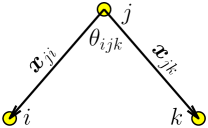
Figure 8: The convention chosen here for angles $\theta_{ijk}$ in 2D.

We next spell out derivatives with respect to shear strain; we consider the transformation of coordinates $\mathitbf x\!\to\!{\bm{H}}(\gamma)\!\cdot\!\mathitbf x$ where $\gamma$ is a shear-strain parameter, and

$${\bm{H}}(\gamma)=\left(\begin{array}[]{cc}1&\gamma\\ 0&1\end{array}\right)\,,$$

then

$$\frac{\partial\theta_{ijk}}{\partial\gamma} = (\mathitbf n_{ji}\cdot\hat{\mathitbf y})^{2}-(\mathitbf n_{jk}\cdot\hat{\mathitbf y})^{2}\,,$$

$$\frac{\partial^{2}\theta_{ijk}}{\partial\gamma^{2}} = 2(\mathitbf n_{jk}\cdot\hat{\mathitbf y})^{3}(\mathitbf n_{jk}\cdot\hat{\mathitbf x})-2(\mathitbf n_{ji}\cdot\hat{\mathitbf y})^{3}(\mathitbf n_{ji}\cdot\hat{\mathitbf x})\,.$$

With these relations, one has

$$\frac{\partial U_{\mbox{\tiny bend}}}{\partial\gamma} = \!\!\!\!\sum_{\mbox{\tiny angles }ijk}\!\!\!\!\!\Phi^{\prime}(\theta_{ijk})\frac{\partial\theta_{ijk}}{\partial\gamma}\,,$$

$$\frac{\partial^{2}U_{\mbox{\tiny bend}}}{\partial\gamma^{2}} = \!\!\!\!\!\sum_{\mbox{\tiny angles }ijk}\!\!\!\!\!\Phi^{\prime\prime}(\theta_{ijk})\bigg{(}\frac{\partial\theta_{ijk}}{\partial\gamma}\bigg{)}^{2}\!\!+\!\!\!\!\!\!\sum_{\mbox{\tiny angles }ijk}\!\!\!\!\!\!\Phi^{\prime}(\theta_{ijk})\frac{\partial^{2}\theta_{ijk}}{\partial\gamma^{2}}\,,$$

Finally the mixed derivatives of the angles read

$$\frac{\partial^{2}\theta_{ijk}}{\partial\gamma\partial\mathitbf x_{i}} = \frac{\mathitbf n_{ji}\!\cdot\!\hat{\mathitbf y}}{r_{ji}}\big{(}2(\mathitbf n_{ji}\!\cdot\!\hat{\mathitbf x})^{2}-1\big{)}\hat{\mathitbf y}-2\frac{(\mathitbf n_{ji}\cdot\hat{\mathitbf x})(\mathitbf n_{ji}\!\cdot\!\hat{\mathitbf y})^{2}}{r_{ji}}\hat{\mathitbf x}\,,$$

$$\frac{\partial^{2}\theta_{ijk}}{\partial\gamma\partial\mathitbf x_{k}} = 2\frac{(\mathitbf n_{jk}\!\cdot\!\hat{\mathitbf x})(\mathitbf n_{jk}\!\cdot\!\hat{\mathitbf y})^{2}}{r_{jk}}\hat{\mathitbf x}-\frac{\mathitbf n_{jk}\!\cdot\!\hat{\mathitbf y}}{r_{jk}}\big{(}2(\mathitbf n_{jk}\!\cdot\!\hat{\mathitbf x})^{2}-1\big{)}\hat{\mathitbf y}\,,$$

$$\frac{\partial^{2}\theta_{ijk}}{\partial\gamma\partial\mathitbf x_{j}} = -\frac{\partial^{2}\theta_{ijk}}{\partial\gamma\partial\mathitbf x_{i}}-\frac{\partial^{2}\theta_{ijk}}{\partial\gamma\partial\mathitbf x_{k}}\,,$$

and then

$$\frac{\partial^{2}U_{\mbox{\tiny bend}}}{\partial\gamma\partial\mathitbf x}=\!\!\!\!\sum_{\mbox{\tiny angles }ijk}\!\!\!\!\!\!\Phi^{\prime\prime}(\theta_{ijk})\frac{\partial\theta_{ijk}}{\partial\gamma}\frac{\partial\theta_{ijk}}{\partial\mathitbf x}+\!\!\!\!\sum_{\mbox{\tiny angles }ijk}\!\!\!\!\!\!\Phi^{\prime}(\theta_{ijk})\frac{\partial^{2}\theta_{ijk}}{\partial\gamma\partial\mathitbf x}\,.$$

References

- Alexander [1998] S. Alexander, Amorphous solids: their structure, lattice dynamics and elasticity, Phys. Rep. 296, 65 (1998).
- Wyart [2005] M. Wyart, On the rigidity of amorphous solids, Ann. Phys. Fr. 30, 1 (2005).
- Wyart et al. [2008] M. Wyart, H. Liang, A. Kabla, and L. Mahadevan, Elasticity of floppy and stiff random networks, Phys. Rev. Lett. 101, 215501 (2008).
- Ellenbroek et al. [2009] W. G. Ellenbroek, Z. Zeravcic, W. van Saarloos, and M. van Hecke, Non-affine response: Jammed packings vs. spring networks, Europhys. Lett. 87, 34004 (2009).
- Wyart [2010] M. Wyart, Scaling of phononic transport with connectivity in amorphous solids, Europhys. Lett. 89, 64001 (2010).
- Broedersz et al. [2011] C. P. Broedersz, X. Mao, T. C. Lubensky, and F. C. MacKintosh, Criticality and isostaticity in fibre networks, Nature Physics 7, 983 (2011).
- Düring et al. [2013] G. Düring, E. Lerner, and M. Wyart, Phonon gap and localization lengths in floppy materials, Soft Matter 9, 146 (2013).
- Mao et al. [2013] X. Mao, O. Stenull, and T. C. Lubensky, Effective-medium theory of a filamentous triangular lattice, Phys. Rev. E 87, 042601 (2013).
- Lerner [2018] E. Lerner, Quasilocalized states of self stress in packing-derived networks, Eur. Phys. J. E 41, 93 (2018).
- Lerner et al. [2014] E. Lerner, E. DeGiuli, G. During, and M. Wyart, Breakdown of continuum elasticity in amorphous solids, Soft Matter 10, 5085 (2014).
- Baumgarten et al. [2017] K. Baumgarten, D. Vågberg, and B. P. Tighe, Nonlocal elasticity near jamming in frictionless soft spheres, Phys. Rev. Lett. 118, 098001 (2017).
- González-López et al. [2023] K. González-López, E. Bouchbinder, and E. Lerner, Variability of mesoscopic mechanical disorder in disordered solids, J. Non-Cryst. Solids. 604, 122137 (2023).
- Giannini et al. [2023] J. A. Giannini, E. Lerner, F. Zamponi, and M. L. Manning, Scaling regimes and fluctuations of observables in computer glasses approaching the unjamming transition, arXiv preprint arXiv:2309.08784 (2023).
- MacKintosh et al. [1995] F. C. MacKintosh, J. Käs, and P. A. Janmey, Elasticity of semiflexible biopolymer networks, Phys. Rev. Lett. 75, 4425 (1995).
- Lindström et al. [2010] S. B. Lindström, D. A. Vader, A. Kulachenko, and D. A. Weitz, Biopolymer network geometries: Characterization, regeneration, and elastic properties, Phys. Rev. E 82, 051905 (2010).
- Head et al. [2003] D. A. Head, A. J. Levine, and F. C. MacKintosh, Deformation of cross-linked semiflexible polymer networks, Phys. Rev. Lett. 91, 108102 (2003).
- Broedersz and MacKintosh [2014] C. P. Broedersz and F. C. MacKintosh, Modeling semiflexible polymer networks, Rev. Mod. Phys. 86, 995 (2014).
- Shivers et al. [2019] J. L. Shivers, S. Arzash, A. Sharma, and F. C. MacKintosh, Scaling theory for mechanical critical behavior in fiber networks, Phys. Rev. Lett. 122, 188003 (2019).
- Düring et al. [2014] G. Düring, E. Lerner, and M. Wyart, Length scales and self-organization in dense suspension flows, Phys. Rev. E 89, 022305 (2014).
- Feng et al. [2016] J. Feng, H. Levine, X. Mao, and L. M. Sander, Nonlinear elasticity of disordered fiber networks, Soft Matter 12, 1419 (2016).
- Sharma et al. [2016] A. Sharma, A. J. Licup, K. A. Jansen, R. Rens, M. Sheinman, G. H. Koenderink, and F. C. MacKintosh, Strain-controlled criticality governs the nonlinear mechanics of fibre networks, Nature Physics 12, 584 (2016).
- Licup et al. [2016] A. J. Licup, A. Sharma, and F. C. MacKintosh, Elastic regimes of subisostatic athermal fiber networks, Phys. Rev. E 93, 012407 (2016).
- Rens et al. [2018] R. Rens, C. Villarroel, G. Düring, and E. Lerner, Micromechanical theory of strain stiffening of biopolymer networks, Phys. Rev. E 98, 062411 (2018).
- Merkel et al. [2019] M. Merkel, K. Baumgarten, B. P. Tighe, and M. L. Manning, A minimal-length approach unifies rigidity in underconstrained materials, Proc. Natl. Acad. Sci. U.S.A. 116, 6560 (2019).
- Shivers et al. [2023] J. L. Shivers, A. Sharma, and F. C. MacKintosh, Strain-controlled critical slowing down in the rheology of disordered networks, Phys. Rev. Lett. 131, 178201 (2023).
- Lerner and Bouchbinder [2023a] E. Lerner and E. Bouchbinder, Scaling theory of critical strain-stiffening in disordered elastic networks, Extreme Mechanics Letters 65, 102104 (2023a).
- Rens and Lerner [2019] R. Rens and E. Lerner, Rigidity and auxeticity transitions in networks with strong bond-bending interactions, Eur. Phys. J. E 42, 114 (2019).
- Kapteijns et al. [2021] G. Kapteijns, E. Bouchbinder, and E. Lerner, Unified quantifier of mechanical disorder in solids, Phys. Rev. E 104, 035001 (2021).
- Jacobs and Thorpe [1996] D. J. Jacobs and M. F. Thorpe, Generic rigidity percolation in two dimensions, Phys. Rev. E 53, 3682 (1996).
- Ellenbroek et al. [2015] W. G. Ellenbroek, V. F. Hagh, A. Kumar, M. F. Thorpe, and M. van Hecke, Rigidity loss in disordered systems: Three scenarios, Phys. Rev. Lett. 114, 135501 (2015).
- Lerner and Bouchbinder [2023b] E. Lerner and E. Bouchbinder, Anomalous linear elasticity of disordered networks, Soft Matter 19, 1076 (2023b).
- Maloney and Lemaître [2004] C. Maloney and A. Lemaître, Subextensive scaling in the athermal, quasistatic limit of amorphous matter in plastic shear flow, Phys. Rev. Lett. 93, 016001 (2004).
- Bitzek et al. [2006] E. Bitzek, P. Koskinen, F. Gähler, M. Moseler, and P. Gumbsch, Structural relaxation made simple, Phys. Rev. Lett. 97, 170201 (2006).
- Rens et al. [2016] R. Rens, M. Vahabi, A. J. Licup, F. C. MacKintosh, and A. Sharma, Nonlinear mechanics of athermal branched biopolymer networks, J. Phys. Chem. B 120, 5831 (2016).
- Wyart et al. [2005] M. Wyart, L. E. Silbert, S. R. Nagel, and T. A. Witten, Effects of compression on the vibrational modes of marginally jammed solids, Phys. Rev. E 72, 051306 (2005).
- Yan et al. [2016] L. Yan, E. DeGiuli, and M. Wyart, On variational arguments for vibrational modes near jamming, Europhys. Lett. 114, 26003 (2016).
- Ellenbroek et al. [2006] W. G. Ellenbroek, E. Somfai, M. van Hecke, and W. van Saarloos, Critical scaling in linear response of frictionless granular packings near jamming, Phys. Rev. Lett. 97, 258001 (2006).
- Silbert et al. [2005] L. E. Silbert, A. J. Liu, and S. R. Nagel, Vibrations and diverging length scales near the unjamming transition, Phys. Rev. Lett. 95, 098301 (2005).
- Rens [2019] R. Rens, Theory of rigidity transitions in disordered materials (PhD thesis, Univeristy of Amsterdam, the Netherlands, 2019).
- Vermeulen et al. [2017] M. F. J. Vermeulen, A. Bose, C. Storm, and W. G. Ellenbroek, Geometry and the onset of rigidity in a disordered network, Phys. Rev. E 96, 053003 (2017).