Localization Is All You Evaluate:
Data Leakage in Online Mapping Datasets and How to Fix It

Adam Lilja^1,2 Junsheng Fu² Erik Stenborg² Lars Hammarstrand²
¹Chalmers University of Technology ²Zenseact
{firstname.lastname}@{chalmers.se, zenseact.com}

Abstract

Data leakage is a critical issue when training and evaluating any method based on supervised learning. The state-of-the-art methods for online mapping are based on supervised learning and are trained predominantly using two datasets: nuScenes and Argoverse 2. These datasets revisit the same geographic locations across training, validation, and test sets. Specifically, over $80$ % of nuScenes and $40$ % of Argoverse 2 validation and test samples are located less than $5$ m from a training sample. This allows methods to localize within a memorized implicit map during testing and leads to inflated performance numbers being reported. To reveal the true performance in unseen environments, we introduce geographical splits of the data. Experimental results show significantly lower performance numbers, for some methods dropping with more than $45$ mAP, when retraining and reevaluating existing online mapping models with the proposed split. Additionally, a reassessment of prior design choices reveals diverging conclusions from those based on the original split. Notably, the impact of the lifting method and the support from auxiliary tasks (e.g., depth supervision) on performance appears less substantial or follows a different trajectory than previously perceived. Link to Geographical splits.

1 Introduction

A core capability for an autonomous vehicle is to estimate the road in its vicinity. There are two complementary approaches for this task: retrieving the information from a pre-built map using localization [5], and directly predicting the online map using onboard sensors like camera and lidar [17]. This work focuses on the latter, online mapping. While a pre-built map provides detailed and accurate information, it also requires robust localization and continuous map updates to be useful. The online mapping approach sidesteps this and instead relies solely on onboard sensors and algorithms. It is thus independent of variations in current surroundings compared to mapped data. The challenge with online mapping instead lies in generalizing to new locations, beyond the places captured in the training data.

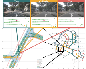
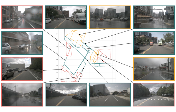
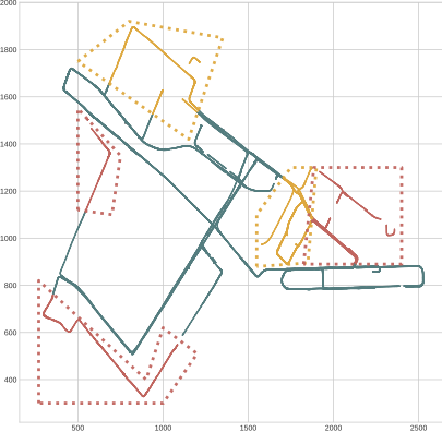
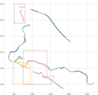
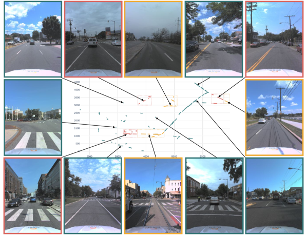
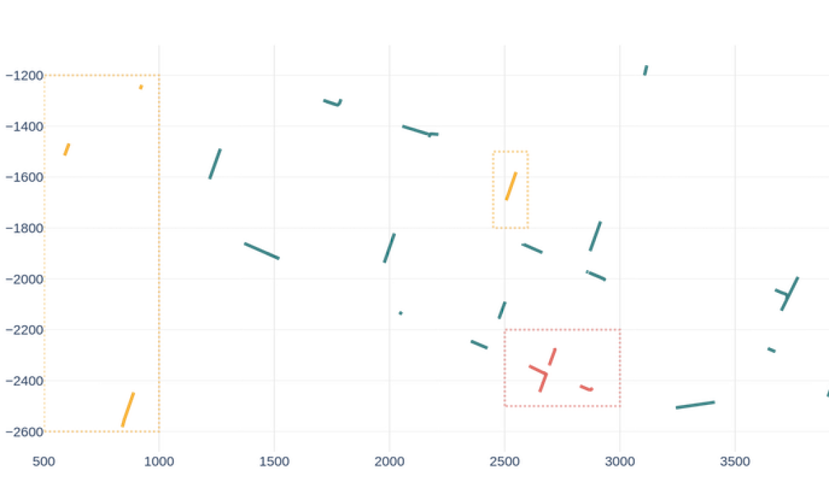
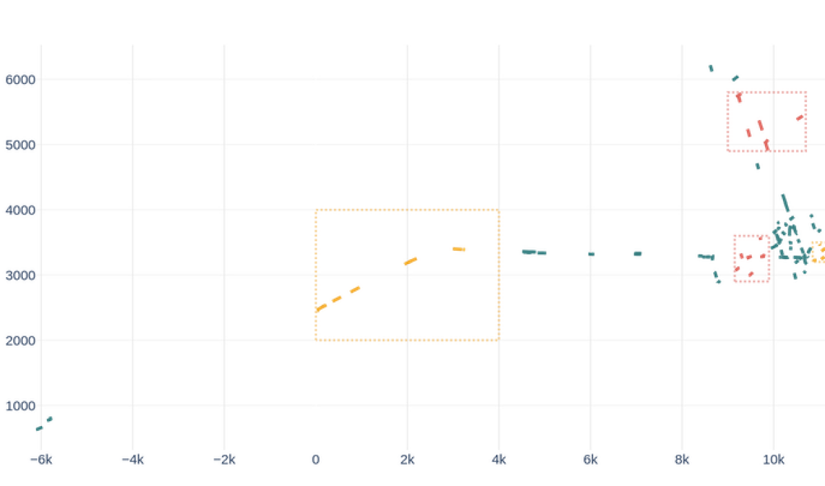
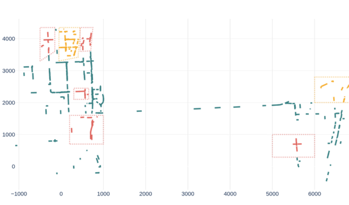
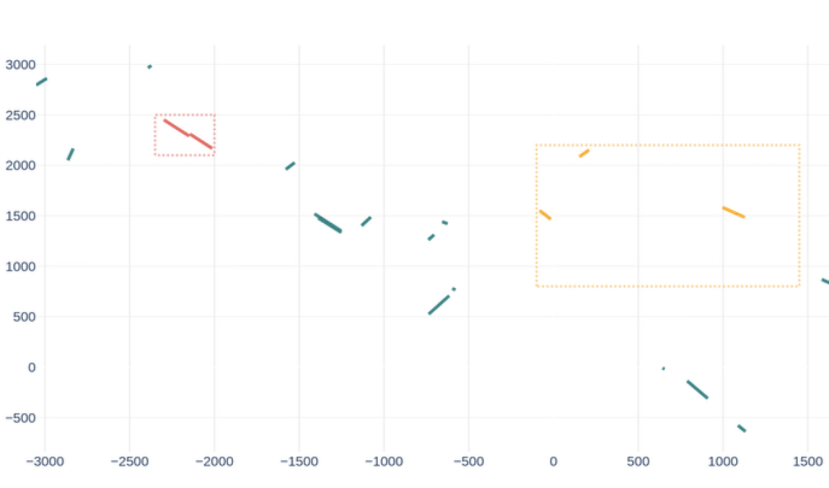
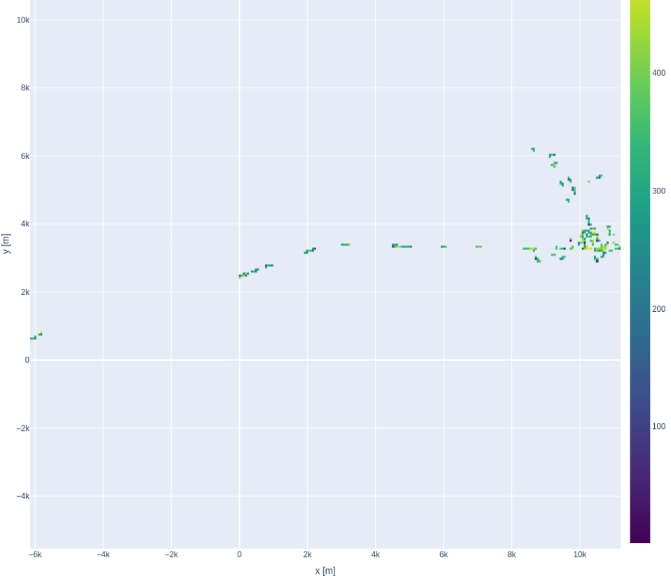
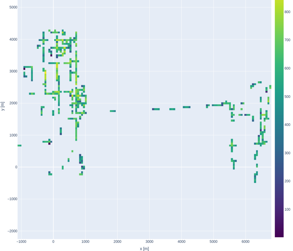
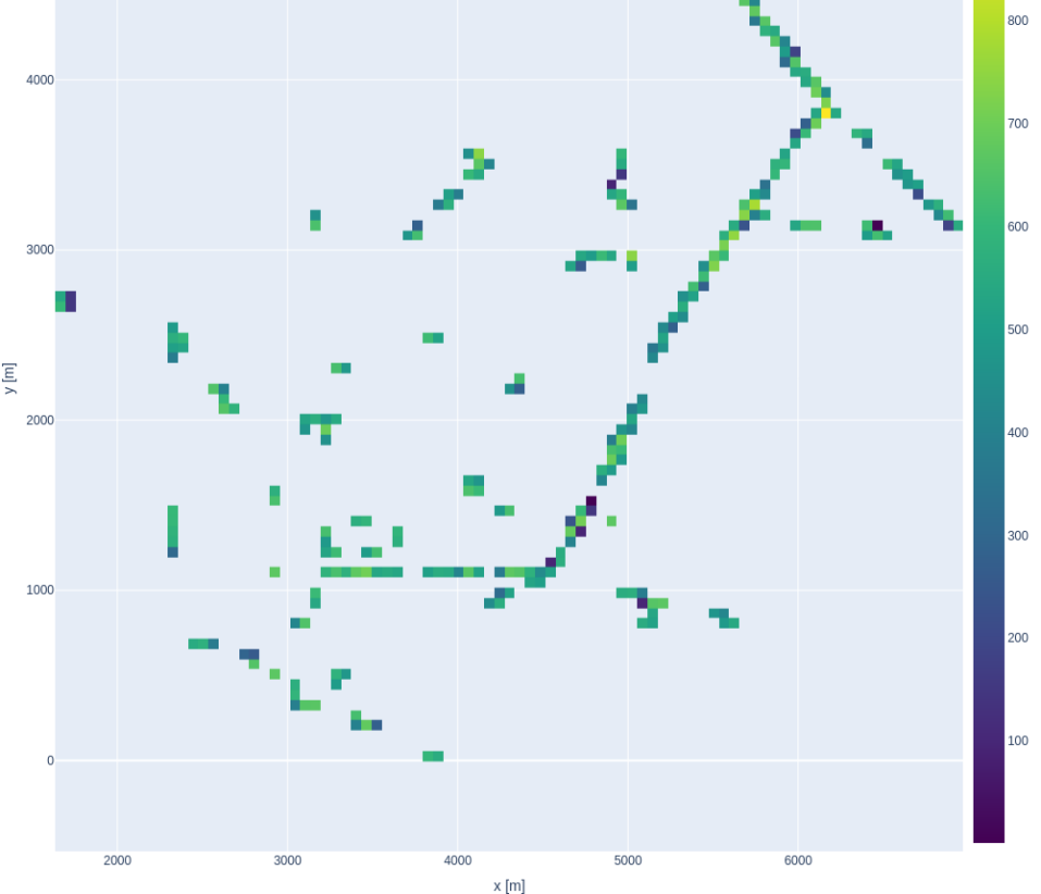
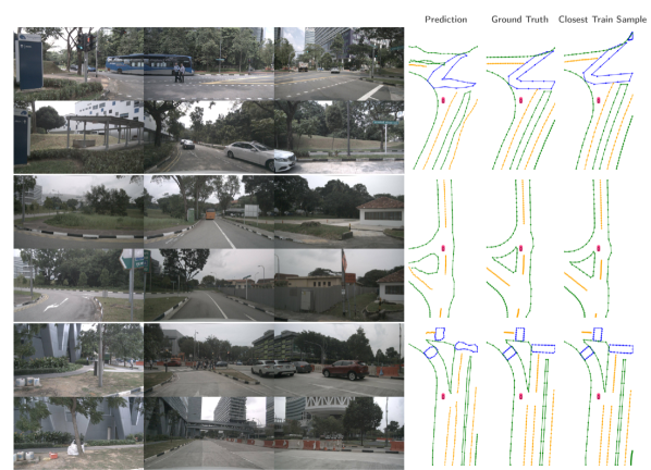
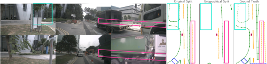
Refer to caption — Figure 1: Example of substantial geographical overlap between train, val, and test sets for nuScenes’ Singapore One-North. Green circle, Orange cross, and Red plus are training, validation, and test samples, respectively.

The current state-of-the-art methods for online mapping are based on supervised learning. While there exist large public datasets [10, 27, 31, 1, 2, 6, 29] that support training of perception and planning models for many of the crucial tasks of an autonomous vehicle, only a few of these provide the HD maps needed to train online mapping models, see Tab. 1. Moreover, as these datasets are mainly constructed to support object detection, object tracking, and motion forecasting tasks, we argue that they, in their original form, are not ideal for training online mapping models for two reasons: (1) The training, validation, and test sets are constructed by splitting the data temporally. This is an easy way to ensure that, e.g., the same vehicle is not present in the same position in the training and test sets yielding fair evaluation of object detection methods. However, since the areas where these datasets are collected are relatively small, the same areas are revisited multiple times. Failing to account for this when dividing the data, results in significant geographical inter-set overlap between the training, validation and test sets as Fig. 1 exemplifies. Fig. 2 further visualizes the input images, prediction, ground truth, and the closest training sample of a test sample for another example. The test sample is very close to the nearest training sample, enabling a method to score well on that test sample by memorizing the image-to-map connection from the training sample, and recalling it at test time. This connection can be created using any features in the images such as buildings and traffic signs. This would rather resemble localizing in a pre-built map and presenting it at test time, than the intended task of online mapping. (2) As each data sample is collected from a data sequence under normal driving, there is substantial intra-set overlap/correlation between the data samples within the sets. This correlation is especially evident near intersections where the vehicle is standing still or driving slowly. Essentially, the ground truth HD maps for close training samples are only slight transformations of the same information. Both of these aspects violate the independent and identically distributed data assumption fundamental in training machine learning models.

In this paper, we show that there is a significant geographical overlap in two of the most commonly used datasets for online mapping, nuScenes [2] and Argoverse 2 [29]. Furthermore, we show that this overlap causes severe inflation in the reported performance of the state-of-the-art methods and, more critically, results in poorer generalizability than initially perceived.

To support future research in the area of online mapping we provide a new balanced geographical split for both nuScenes and Argoverse 2, where the overlap is minimized while maintaining the original diversity in terms of e.g., weather and time of day. We re-evaluate state-of-the-art methods trained on our proposed geographical splits to give a more representative view of their performance. Additionally, we perform more detailed experiments to investigate how the large overlap has affected conclusions regarding important algorithmic choices, e.g., the type of lifting method used to go from perspective camera view to bird’s eye view.

2 Related Work

Current works on online mapping can be divided into two tracks, segmentation-based maps and vector-based maps, differing mainly in how the online map is represented. In segmentation-based maps, the aim is to predict a rasterized bird’s eye view map where each cell is classified as, e.g., empty, lane marking and road edge. For vector-based methods, the predicted map is described by a set of objects with a given class and which geometry is described by a vector of point coordinates, i.e., a polyline. Both families of methods use supervised learning, and as such, depend heavily on the datasets used to train them.

2.1 Segmentation-based Online Mapping

The current segmentation-based online mapping methods [22, 24, 30, 15, 19, 9, 14, 7, 12, 32, 21] universally adopt a core technique known as lifting. This entails converting image features from perspective view (PV) to Bird’s Eye View (BEV) features, from which the segmented map is directly predicted. The primary challenge for these methods lies in accurately mapping features from the perspective view to their corresponding locations in BEV due to the absence of depth information in images. Various learnable lifting methods have been proposed, broadly categorized as either pulling the features to BEV from PV, or pushing the features from PV to BEV.

In essence, pulling methods aim to retrieve features from PV based on dense queries in BEV [7, 15, 33, 21]. A straightforward approach is the Inverse Perspective Mapping (IPM) [20] and involves projecting predefined points in BEV into PV using camera parameters and interpolating features from these projected positions. Alternatively, methods like Geometry-Guided Kernel Transformer (GKT) [7] and BEVFormer [15] use a combination of geometry and attention mechanisms to efficiently pull features to BEV-space. Cross-View Transformer (CVT) [33], in contrast, pulls features without an intermediate BEV representation using cross-attention with a canonical form of all camera views.

The pushing methods used in, e.g. [22, 24, 30, 19, 9, 14], specialize in learning how to map PV features to BEV. Among them, depth-based approaches aim to learn the depth distribution for each image pixel to accurately project PV features. For instance, LSS [22] tries to learn a categorical depth distribution for each pixel and use it to weigh how much of the corresponding PV feature should influence the corresponding BEV-cell. Pyramid Occupancy Network (PON) [24] uses a multi-scale dense transformer for low-resolution BEV projection, employing deconvolutions for upsampling predictions, whereas HDMapNet [14] learns BEV projection through a Multilayer Perceptron (MLP).

Except [24], all these works are at least partly trained and evaluated on data having considerable geographical inter-set overlap severely limiting the validity of conclusions drawn regarding their performance on online mapping tasks. We are thus interested in understanding how segmentation-based online mapping methods are affected by the inter-set overlap of nuScenes and Argoverse 2 and investigating if there is a difference in how well the lifting methods can generalize when evaluated on a geographically separated test and validation set.

2.2 Vector-based Online Mapping

A more efficient representation for online mapping that is more suitable for downstream tasks emerges through a vector-based approach [14, 18, 16, 26, 17], where the position and shape of each object, such as lane or road dividers, is described as a set of connected points. This representation was first introduced in HDMapNet [14] as a handcrafted post-processing step on the predicted segmented map. Subsequent methods extended this representation to be end-to-end trainable. For example, VectorMapNet [18] uses IPM [20] for lifting image features to BEV from which a transformer decoder predicts coarse object representations. These are then refined in a joint Autoregressive Transformer (ART) that attends the coarse prediction and all BEV features. MapTR [16] utilizes GKT [7] for lifting and a DETR-like [4] transformer decoder for predicting the objects. More specifically, they use deformable attention to attend BEV features with hierarchical queries to predict a collection of objects defined by a set of points. MapTRv2 [17] builds on its predecessor, but uses LSS[22] as a lifting method and adds PV depth estimation and segmentation in both PV and BEV as auxiliary supervision.

As with the segmentation-based methods, these methods are primarily evaluated on the original nuScenes and Argoverse 2 splits with considerable inter-set overlap. To give a fairer view of their performance on the intended problem setting, we re-evaluate them on our proposed splits and analyze the results.

2.3 Online Mapping Datasets

Dataset	Source	Main Map Purpose	#Samples			Geo. Split
Dataset	Source	Main Map Purpose	Train	Val	Test	Geo. Split
Argoverse 1 [6]	argo1	OD/MF	$39$ k	$15$ k	$13$ k	✓
Argoverse 2 [29]	argo2	OD/MF	$110$ k	$24$ k	$24$ k	✗
nuScenes [2]	nuSc	OD/MF	$28$ k	$6$ k	$6$ k	✗
nuScenes^⋆ [2]	nuSc	OD/MF	$134$ k	$29$ k	$26$ k	✗
Waymo [27]	Way	OD/MF	$122$ k	$30$ k	$40$ k	✗
Coarse [24]	nuSc	OM	$26$ k	$2$ k	$6$ k	✓
Geo.-nuScenes	nuSc	OM	$28$ k	$6$ k	$6$ k	✓
Geo.-nuScenes^⋆	nuSc	OM	$130$ k	$30$ k	$29$ k	✓
Geo.-Argo	argo2	OM	$110$ k	$24$ k	$24$ k	✓

Table 1: Overview of datasets used for Online Mapping. Our proposed splits are shown in bold. OD = Object Detection, MF = Motion Forecasting, TP = Trajectory Planning, OM = Online Mapping. ^⋆ indicates the densely sampled version.

Split	nuScenes		Argoverse 2
Split	Val	Test	Val	Test
Orig.	$79.4$ %	$85.5$ %	$45.0$ %	$41.9$ %
Coarse [24]	$85.3$ %	$0.0$ %
Geo.	$0.9$ %	$1.1$ %	$0.0$ %	$0.0$ %

Table 2: Ratios of validation and test samples within

5

m of training samples. The Geographical (Geo.) split has negligible overlap compared to the, greatly overlapping, Original (Orig.) split in both nuScenes and Argoverse 2. The coarse split on nuScenes from [24] only has a high overlap in the validation set.

A summary of existing datasets used for online mapping is provided in Tab. 1. Three original datasets provide the HD-maps required to enable the training of online mapping models, Argoverse [6, 29], nuScenes [2] and Waymo [27]. Common for all these primary datasets is that they are mainly intended for object detection and motion forecasting tasks, and, in addition to supplying HD maps, these datasets provide rich annotations for dynamic objects. The datasets provide predefined data splits to ensure equitable and consistent evaluations across different studies utilizing them. It is, however, essential to note that these splits were tailored for dynamic object perception, rather than online mapping. Specifically, they are temporally divided, ensuring that samples from a given sequence do not overlap across multiple sets. However, this does not guarantee that all samples from the same geographical area will be in the same set. Despite this, especially nuScenes [2] and Argoverse 2 [29] have been extensively used for training online mapping models and have become the de facto standard. For example, online mapping methods using nuScenes include [14, 7, 33, 22, 24, 30, 13, 15, 19, 9, 25, 12, 23, 32, 21, 3] and Argoverse 2 is used in [18, 26, 16, 17].

The nuScenes dataset contains $1\,000$ driving sequences collected in two cities (Boston and Singapore) with an area coverage of about $5$ km² [27] and captures different types of city roads as well as containing diverse weather and illumination conditions. In total, the sequences comprise $40\,000$ ( $2$ Hz) key-frame samples with object annotations. These samples have been used for training object detection methods and online mapping methods have adhered to this convention, utilizing the same set of samples for their training. However, in addition to the key-frame samples, intermediate raw sensor data is provided at the rate of the individual sensors, e.g., $12$ Hz for the cameras and $20$ Hz for the lidar, but without object annotations. In support of training online mapping methods, these too provide accurate vehicle pose for all samples in a 2D HD map with information on drivable area, road boundaries, lane dividers, pedestrian crossings, walkways, stop lines, and more. Based on these additional samples we construct a densely sampled nuScenes dataset, and as Tab. 1 shows, contains almost $190\,000$ samples with synchronized image and lidar data. Even though it is possible to train online mapping methods on the complete set, all methods listed above train and evaluate on the much fewer annotated data samples. Furthermore, these samples are located near each other across the different sets as the same geographical position is re-visited multiple times. Fig. 1 illustrates a single example, where the proximity of validation and test samples to training samples is evident. Further analysis, as Tab. 2 depicts, reveals that approximately $80\%$ and $85\%$ of validation and test samples, respectively, are within $5$ meters of a sample used during training.

The other prominently used dataset, Argoverse 2, is an extension of the 2019 version Argoverse [6]. In contrast to its predecessor, Argoverse 2 is not geographically split, but is much larger and collected from 6 U.S. cities with an area coverage of $17$ km² [1]. It comprises $1\,000$ annotated driving sequences, which are on average $15$ s long and annotated at $10$ Hz. Each sample offers observations from similar sensors as nuScenes, albeit in a slightly different configuration, and the provided HD maps are in 3D, but with a focus on drivable area, road boundaries, lane dividers, and pedestrian crossings. By inspecting Argoverse 2, one can see that it too suffers from a considerable level of inter-set geographical overlap. Tab. 2 shows that approximately $45\%$ and $42\%$ of the validation and test samples are within a $5$ m range of the closest train sample.

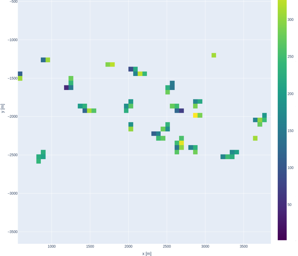
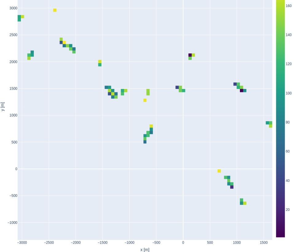
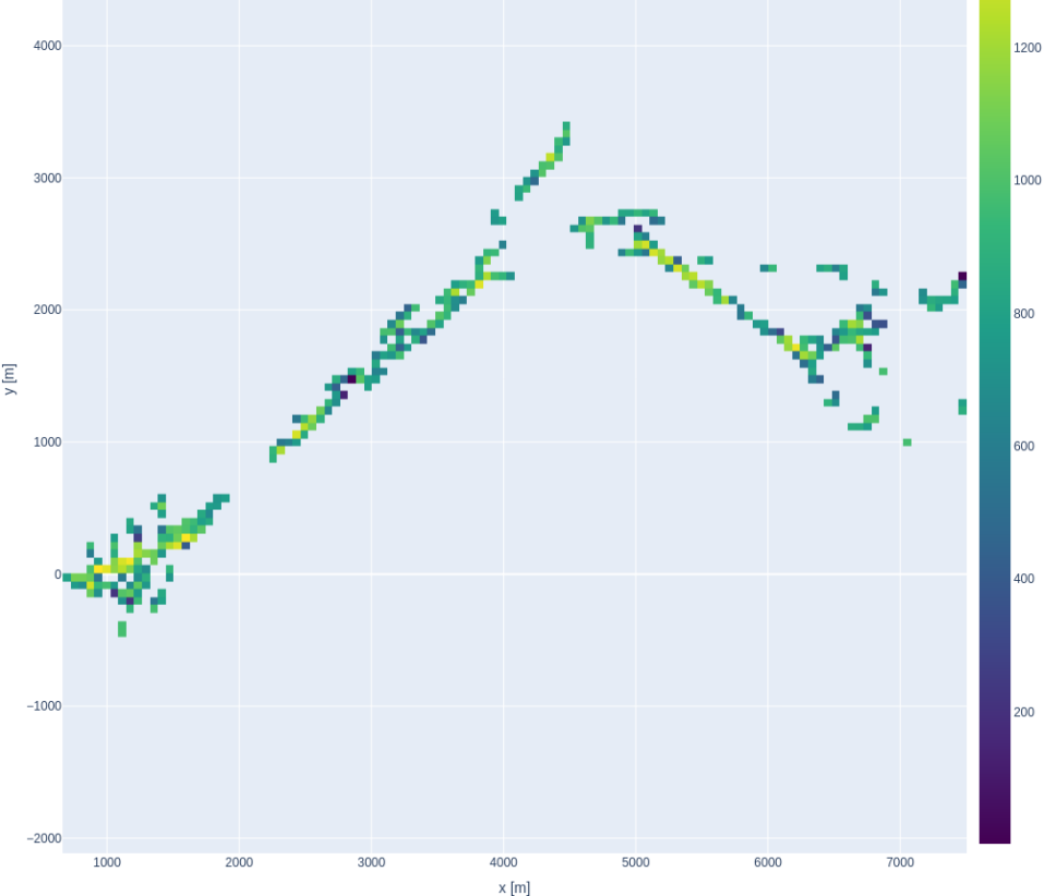
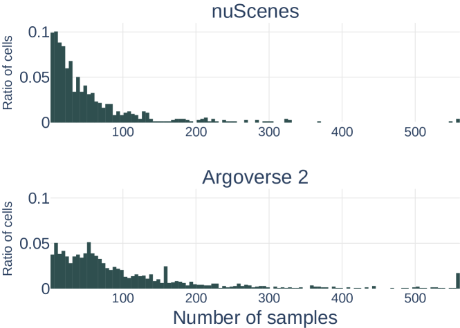
Comparing nuScenes and Argoverse 2, we note that the inter-set sample overlap is larger for nuScenes, and that Argoverse 2 boasts a larger number of samples and a more extensive coverage area. Another difference arises from Argoverse 2 being densely sampled, resulting in less spatial variation and a higher intra-set sample density. The discrepancy is highlighted in Fig. 3, where samples are discretized into cells with a side length of $60$ meters, the typical evaluation range for most online mapping methods, e.g. [14, 18, 16, 26, 17]. The distribution of non-empty cells over the number of samples they contain has more probability mass with the higher counts for Argoverse 2. Despite Argoverse 2 having nearly four times the number of samples compared to nuScenes, the number of non-empty cells is only $1.7$ times higher.

2.4 Geographical Data Splits

To the best of the author’s knowledge, for nuScenes there are two approaches to address the issue of geographical inter-set overlap, whereas for Argoverse 2 there is none. One approach is to simply divide training, validation, and test according to the different locations [23]. Although this is a valid split set, it also significantly increases the difficulty of the problem as evidenced by the poor evaluation result presented in the paper. For instance, within nuScenes, the Boston scenes are quite distinct from the Singapore ones. The distinctions encompass not just lane marker types and weather conditions but also driving on opposite sides of the road. Another, perhaps more evenhanded splitting approach is used in [24], where the authors acknowledged the need for a geographically divided train and test split when evaluating their online mapping method (PON) on nuScenes. They coarsely partition the sets along large, visually similar, neighborhoods, limiting the diversity within each set. Furthermore, their proposed geographical split does not take the validation set into account (see Tab. 2) and discards samples from the original test set reducing the total size of the dataset. In the rest of this paper, we refer to this split as coarse as in, e.g., Tab. 1.

3 Proposed Geographical Data Split

To provide balanced geographical training, validation, and test sets of nuScenes and Argoverse 2, we split the data according to the samples’ geographical positions leading to diminishing inter-set overlap. We make use of the original splits’ testing data as the map is provided for those samples. The proportions of the splits are $70$ %, $15$ %, and $15$ % for training, validation, and test sets respectively.

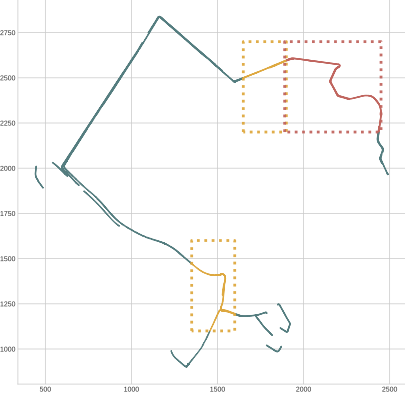
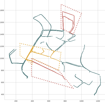
In order to preserve diversity in zone classes (in the urban planning sense, e.g., residential, commercial, and industrial) but also maintain the frequency of road object classes, weather conditions, and time of day a fine-grained and thorough partitioning is performed. Our splits are meticulously designed to ensure a proportional representation of samples from these criteria in each set, mirroring the distribution in the full dataset, and ensuring all cities are well-represented. This has been done by manually checking the maps, their samples and attributes, to define regions within which all samples are put in a specified set. Splits are visualized Appendix B and are available on the project webpage.

While partitioning the data, we did not account for the intra-set overlap discussed in Sec. 2.3. Even though not affecting the splitting process, we acknowledge its potential importance and believe it warrants consideration in the utilization of these datasets. However, the specifics of how to address this concern and the associated implications are left for future research. We realize that the use of original test data has implications for multi-task networks (e.g. also performing object detection) and have thus also ensured that balance remains among the sets when removing the original test data. The number of samples in each set and an overview of our proposed splits for nuScenes and Argoverse 2 can be seen in Tab. 1.

3.1 nuScenes

Splitting nuScenes on a sequence level requires grouping large areas with similar zone classes together and putting them in a single set, as seen in [22]. This is due to the entangled nature of the sequences where many partially overlap. Instead of assigning entire $20$ s sequences, we assign each sample individually to a set. However, as we want to maintain the usefulness for object detection and keep the possibility of using the data for temporal fusion, having consecutive samples is important. We have thus tried to keep the number of sequences being cut into multiple parts as low as possible, making the cuts, when necessary, across the road’s driving direction. Further discussion and examples can be found in Appendix A.

Tab. 2 displays the ratio of validation and test samples being within $5$ m of a training sample for the proposed geographical split. Our suggested geographical splits show only minimal overlap. The remaining overlap is due to the samples close to the above-mentioned cut-off regions between sets. To see the effects of these samples we do experiments where these samples have been filtered out and see that their impact is negligible. Appendix A in the supplementary material covers more details.

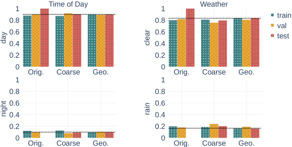
It is also important that the weather conditions and time of day are equally distributed through the sets. While both the original and coarse splits are imbalanced, Fig. 4 details that our geographical split is balanced across all attributes.

3.2 Argoverse 2

The sequences in the Argoverse 2 dataset are more spread out compared to nuScenes, and a balanced sequence-wise split is possible to obtain. There is thus no impact on usability for object detection, object tracking, and other temporal fusion applications for this split. As Tab. 2 presents, we get no validation or test samples within $5$ m of a training sample.

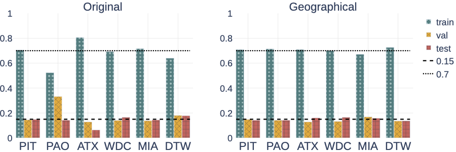
Unfortunately, attributes concerning the conditions associated with the different sequences are not available for Argoverse 2 making it hard to do a quantitative analysis. Our main focus is thus to give a balanced geographical split, partitioning areas with similar zone classes equally in the different sets. Fig. 5 illustrates the distribution of the number of samples in each city, and Appendix B highlights the geographical distribution.

4 Experiments

nuScenes	Model	S	Back- bone	Lifting	Decoder	Split	Divider		Boundary		Crossing		Mean
	Model	S	Back- bone	Lifting	Decoder	Split	Val	Test	Val	Test	Val	Test	Val	Test
	VectorMapNet	C	R50	IPM	ART	Orig	$48.9$	$47.9$	$40.9$	$63.8$	$39.8$	$52.8$	$43.2$	$54.8$
	VectorMapNet	C	R50	IPM	ART	Geo	$13.5$	$17.3$	$14.9$	$21.6$	$13.7$	$15.7$	$14.0$	$18.2$
	MapTR	C	R18	GKT	DETR	Orig	$38.0$	$52.2$	$37.2$	$46.0$	$24.2$	$28.9$	$33.1$	$42.4$
	MapTR	C	R18	GKT	DETR	Geo	$10.6$	$12.1$	$13.7$	$20.1$	$5.1$	$1.0$	$9.8$	$11.1$
	MapTR	C	R50	GKT	DETR	Orig	$51.0$	$65.8$	$52.6$	$60.5$	$43.0$	$53.3$	$48.8$	$59.9$
	MapTR	C	R50	GKT	DETR	Geo	$16.0$	$19.9$	$26.7$	$33.3$	$14.4$	$5.9$	$19.0$	$19.7$
	MapTRv2	C	R50	LSS	DETR	Orig	$61.8$	$77.3$	$63.7$	$70.9$	$59.1$	$69.8$	$61.5$	$72.7$
	MapTRv2	C	R50	LSS	DETR	Geo	$20.9$	$23.4$	$32.6$	$40.5$	$26.5$	$14.8$	$26.7$	$26.2$
	MapTRv2	CL	R50 2nd	LSS	DETR	Orig	$54.9$	$70.5$	$55.1$	$63.9$	$51.9$	$63.1$	$54.0$	$65.8$
	MapTRv2	CL	R50 2nd	LSS	DETR	Geo	$15.1$	$18.0$	$27.4$	$35.2$	$17.4$	$7.0$	$20.0$	$20.1$
Argoverse 2	VectorMapNet 2D	C	R50	IPM	ART	Orig	$51.9$	$46.8$	$42.1$	$40.7$	$38.0$	$38.7$	$44.0$	$42.0$
	VectorMapNet 2D	C	R50	IPM	ART	Geo	$39.8$	$35.0$	$31.5$	$32.4$	$26.8$	$31.3$	$32.7$	$32.9$
	MapTR 2D	C	R50	GKT	DETR	Orig	$64.0$	$62.8$	$63.2$	$61.0$	$63.7$	$62.4$	$63.6$	$62.1$
	MapTR 2D	C	R50	GKT	DETR	Geo	$50.0$	$45.2$	$47.5$	$48.3$	$46.6$	$50.9$	$48.0$	$48.2$
	MapTRv2 2D	C	R50	LSS	DETR	Orig	$71.7$	$68.9$	$67.0$	$63.8$	$64.5$	$63.1$	$67.7$	$65.3$
	MapTRv2 2D	C	R50	LSS	DETR	Geo	$58.4$	$56.6$	$51.3$	$53.5$	$49.7$	$55.6$	$53.1$	$55.2$
	MapTRv2 3D	C	R50	LSS	DETR	Orig	$68.7$	$66.0$	$64.3$	$61.7$	$59.6$	$58.7$	$64.2$	$62.1$
	MapTRv2 3D	C	R50	LSS	DETR	Geo	$56.2$	$55.0$	$47.8$	$51.0$	$46.2$	$51.8$	$50.1$	$52.6$

Table 3: mAP comparison across various methods trained on Original (Orig) and Geographical (Geo) splits. Sensors denoted as Camera [C] and Lidar [L], Backbones include Resnet18 [R18], Resnet50 [R50], and SECOND [2nd], and Decoders are Autoregressive Transformer [ART] and Object Detection with Transformer [DETR]. The performance of all methods shows a significant drop when trained and evaluated on geographically split data, with blue indicating higher values and yellow indicating lower values.

To demonstrate the geographical data leakage problem with using original splits of nuScenes and Argoverse 2, we evaluate the performance of state-of-the-art online mapping methods on both the original and proposed geographical data splits. Additionally, we investigate the effects of the dataset size and re-validate studies performed in previous works.

In our experiments, unless specified, no modifications have been made to the configurations of the evaluated methods, and we direct readers to the respective papers for specific training details. Additionally, the performance is measured using standard practice in the respective field, i.e., Intersection over Union (IoU) for segmentation-based methods and mean average precision (mAP) [14] for vector-based methods. For the latter, the average precision $\text{AP}_{\tau}$ is calculated through thresholding the Chamfer distance between matched prediction/ground truth-pairs for the thresholds $\tau\in T,T=\{0.5,1.0,1.5\}$ to get

\text{mAP}=\frac{1}{|T|}\sum_{\tau\in T}\text{AP}_{\tau}.

(1)

We report mAP both for individual object classes as well as their average.

4.1 Data Leakage Effects

To investigate the effects of a geographical overlap across data partitions, we train several methods on both the original and geographical splits. We do this separately for vector-based and segmentation-based methods.

Tab. 3 reports the results for vector-based methods. Across all evaluated methods we see a significant performance drop when using geographical splits compared to the original splits. On average the performance slide is more than $35$ mAP and $12$ mAP for nuScenes and Argoverse 2, respectively. Moreover, the effect is consistent over all lifting methods, sensor modalities, and decoders, but the ranking among the evaluated methods remains. It can also be seen that the performance drop remains consistent when adding lidar or considering the 3D geometry of the online map.

The best-performing method (MapTRv2) on nuScenes using images as input drops from an mAP of $72.7$ to just $26.2$ , showcasing a significant difference of $46.5$ mAP, when trained and evaluated appropriately. The drop is less pronounced, although still significant, on Argoverse 2, decreasing from $65.3$ to $55.2$ mAP. In general, the impact of the split is particularly pronounced for methods trained on nuScenes. In light of these findings, we conclude that the smaller size of nuScenes, although convenient, makes it inadequate for training current online mapping methods. Moreover, although Argoverse 2 has more samples, it’s somewhat surprising that algorithms trained on it still exhibit substantially improved generalization ability considering that the intra-set overlap is also larger. We hypothesize that, despite the intra-set overlap being greater, this overlap doesn’t hinder training; instead, it possibly functions as natural and beneficial data augmentation similarly as synthetic augmentations have shown to be highly useful for image classification and object detection tasks [8].

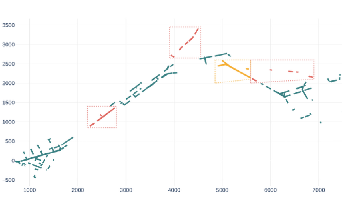
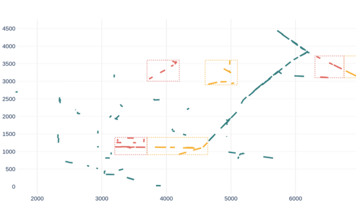
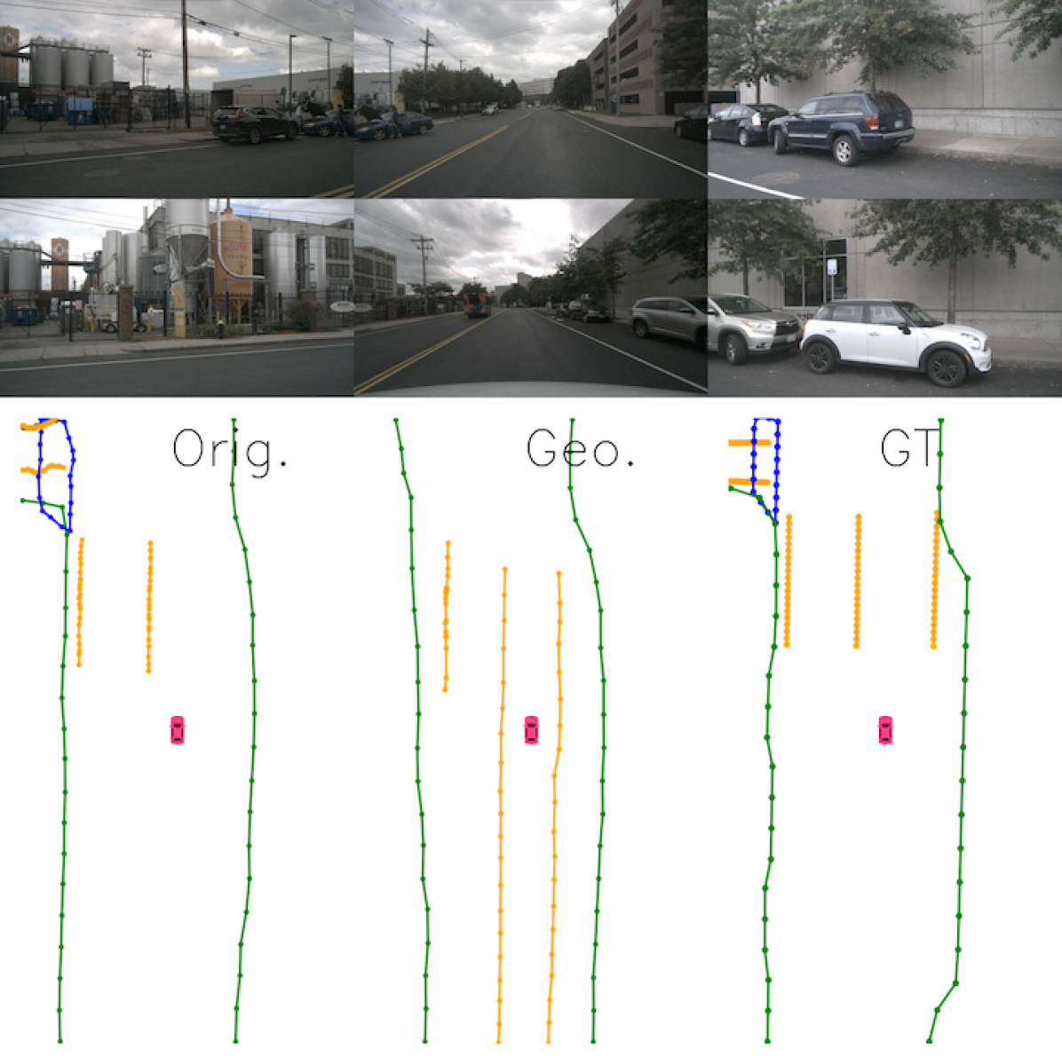
To illustrate the significance of these numbers, a qualitative example is provided in Fig. 6, comparing MapTR [16] predictions on a validation sample when trained on the original and the geographical nuScenes splits. Studying the figure carefully, we can see that the model trained on the original split accurately predicts the road edge (green line) even for areas completely occluded in the images, highlighted by the red box. The method can also predict the lane divider (yellow line) on the opposing road through the trucks and barriers, as highlighted in the pink box. As these methods are single-shot inferences and do not consider previous sensor observations, it is unreasonable that they can accurately predict road structures that are not visible or clearly indicated by other structures in the current view. The method appears to predominantly learn to localize validation and test samples within the provided training map. This is by no means unique to this particular method or this example, but rather a consequence of the overlap between train and evaluation sets. More qualitative examples are provided in Appendix C.

For segmentation-based methods, Tab. 4 shows reduced performance for multi-class (divider, boundary, and crossing segmentation) predictions when trained on geographically split data. This suggests that the impact extends beyond vectorized methods. In this experiment, HDMapNet is kept the same as from the original paper, whereas for the others we adapt the lifting techniques, namely Inverse Perspective Mapping (IPM), Cross-View Transformer (CVT) and Geometry-Guided Kernel Transformer (GKT) to predict dividers, boundaries, and pedestrian crossings. Architectural details such as the image feature extraction backbone, Efficientnet-b4 [28], and segmentation decoder from SimpleBEV [11] are kept the same for all lifters for fair comparison. As for the vector-based online mapping methods, the drop is larger on nuScenes than Argoverse 2 and the ranking among methods remains largely unchanged.

	Model	Split	Divider		Boundary		Crossing		Mean
	Model	Split	Val	Test	Val	Test	Val	Test	Val	Test
nuScenes	GKT	Orig.	25.8	25.4	25.6	22.7	6.2	5.1	19.2	17.7
	GKT	Geo.	12.5	17.9	12.6	16.9	1.4	1.9	8.8	12.3
	CVT	Orig.	30.9	30.1	30.5	25.5	11.7	7.6	24.4	21.1
	CVT	Geo.	16.9	11.6	17.0	10.3	4.5	1.1	12.8	7.7
	IPM	Orig.	46.8	52.4	50.0	52.8	26.8	27.4	41.2	44.2
	IPM	Geo.	29.6	29.4	36.2	33.6	16.2	9.7	27.4	24.2
	HDMapNet	Orig	38.3	47.5	35.5	41.2	20.1	27.6	31.3	38.8
	HDMapNet	Geo	8.6	24.0	22.1	25.4	10.6	14.1	17.1	21.2
Argoverse 2	GKT	Orig.	37.3	28.2	31.4	28.3	10.3	5.7	26.3	20.7
	GKT	Geo.	32.7	29.0	26.2	23.2	8.7	1.5	22.5	17.9
	CVT	Orig.	40.1	29.4	32.0	29.3	12.1	7.1	28.4	21.9
	CVT	Geo.	35.1	31.7	26.5	28.5	10.9	1.4	24.2	20.5
	IPM	Orig.	58.5	45.7	50.6	50.1	33.4	32.4	47.5	42.7
	IPM	Geo.	50.5	39.1	44.1	45.2	29.7	28.8	41.5	37.7

Table 4: Multi-class map segmentation on the datasets, evaluating performance with IoU. The performance drops for all methods when using the Geographical (Geo.) versus the Original (Orig.) split. Similarly as for the vector-based online mapping methods the drop is larger on nuScenes than Argoverse 2.

Overall, the geographical split yields a more consistent performance between the validation and test sets compared to the original split. This suggests a balanced distribution of samples across sets, a crucial consideration when selecting hyperparameters using the validation set. This balance facilitates drawing more reliable conclusions about hyperparameter choices, ensuring that insights gained from the validation set are likely to generalize well to the test set.

4.2 Dataset Size

To further investigate the effects of the amount of data, we perform experiments when the validation data is injected into the training data. Additionally, we explore the effects of training with the entire densely sampled nuScenes dataset, matching the sample count of the Argoverse 2 dataset but without expanding the geographic coverage of the samples.

Training set extension

When extending the training set with the validation samples, effectively increasing the training set with $20$ %, Tab. 5 shows a boost in the test performance for both segmentation- and vector-based methods. The impact is greater on nuScenes, but Argoverse 2 also benefits from the added data. Indicating that more extensive datasets are necessary for learning online mapping. For instance, the extra data has a higher impact for MapTR on Argoverse 2, $+1.4$ mAP, than the choice of lifting method, $+0.7$ mAP. On nuScenes, the impact is greater, but also similarly large as using LSS in comparison to GKT for lifting, $+1.9$ and $+2.0$ respectively. The lifting methods are further discussed in Sec. 4.3 and shown in Tab. 7.

	Model	Split	Divider	Boundary	Crossing	Mean
nuScenes	HDMapNet	Geo	$15.3$	$17.3$	$9.0$	$13.9$
	HDMapNet	Geo $\cup$	$24.4$	$26.3$	$14.7$	$21.8$
	VectorMapNet	Geo	$17.3$	$21.6$	$15.7$	$18.2$
	VectorMapNet	Geo $\cup$	$18.8$	$25.3$	$17.6$	$20.6$
	MapTR	Geo	$19.9$	$33.3$	$5.9$	$19.7$
	MapTR	Geo $\cup$	$21.9$	$36.1$	$6.8$	$21.6$
	MapTRv2	Geo	$23.4$	$40.5$	$14.8$	$26.2$
	MapTRv2	Geo $\cup$	$25.3$	$42.1$	$18.6$	$28.7$
Argoverse 2	VectorMapNet	Geo	$35.0$	$32.4$	$31.3$	$32.9$
	VectorMapNet	Geo $\cup$	$37.5$	$33.1$	$32.7$	$34.4$
	MapTR	Geo	$45.2$	$48.3$	$50.9$	$48.2$
	MapTR	Geo $\cup$	$47.3$	$49.4$	$52.0$	$49.6$
	MapTRv2	Geo	$56.6$	$53.5$	$55.6$	$55.2$
	2D	Geo $\cup$	$59.5$	$54.7$	$53.4$	$55.9$

Table 5: Increasing training data by

15

% using the union of training and validation samples, marked by

\cup

, improves test performance. IoU for HDMapNet and mAP for the other methods.

Dense nuScenes

Furthermore, we investigate the effect of training MapTRv2 using the densely sampled data. We adjust the number of training epochs for the densely sampled training such that the total number of optimizer steps is similar to the sparsely sampled data. Tab. 6 reports the result of this training and how it compares to training on sparse data. There is a distinguished increase in performance on the original split, achieving up to a 24.9 mAP improvement on the validation set by utilizing the densely sampled data. However, the method’s performance on the Geographical split sees marginal improvement, with a maximum increase of only 0.7 mAP.

Split	Train Sampling	Divider		Boundary		Crossing		Mean
Split	Train Sampling	Val	Test	Val	Test	Val	Test	Val	Test
Orig.	Sparse	$61.8$	$77.3$	$63.7$	$70.9$	$59.1$	$69.8$	$61.5$	$72.7$
Orig.	Dense	$90.3$	$89.7$	$84.4$	$84.5$	$86.4$	$88.3$	$86.4$	$87.5$
Geo.	Sparse	$20.9$	$23.4$	$32.6$	$40.5$	$26.5$	$14.8$	$26.7$	$26.2$
Geo.	Dense	$21.7$	$24.1$	$34.1$	$40.9$	$25.7$	$15.9$	$27.2$	$26.9$

Table 6: Performance comparison of MapTRv2 trained on sparse and dense nuScenes datasets, evaluated on sparse validation and test sets. Utilizing extra samples between key-frames results in a significant performance increase of

24.9

and

14.8

for validation and test, respectively, on the Original split (Orig.). The Geographical split (Geo.) experiences only a marginal performance improvement.

4.3 Re-validation

As the original works validate their design choices and hyperparameter selections on poorly separated training and validation data, it is highly relevant to revisit these validation results to check if the conclusions apply to the proposed geographical split. Although it is not possible to re-run all tests, we try to highlight some interesting observations.

Hyperparameters

We searched alternative hyperparameters for MapTRv2 on the Geographical splits on nuScenes and Argoverse 2, focusing on hyperparameters related to overfitting on the training set, i.e., weight decay, learning rate, and training epochs. Interestingly, although we could observe minor differences the ones initially employed for training on the original split proved equally effective for the Geographical split.

Ablation: Lifting method

In [16], the authors use nuScenes to perform an ablation study on the effect of different lifters on the performance of MapTR, where GKT gives the best results. In Tab. 7, we re-run this test and in contradiction to the previous conclusion, we find the BEVFormer lifter performing slightly better than GKT. However, the differences between the lifters are small making it difficult to conclude the superiority of any of them.

Ablation: Auxiliary tasks

For MapTRv2 [17], we re-ablate the proposed auxiliary tasks in Tab. 8. For nuScenes, we note that, in contrast to conclusions based on the original split, the addition of depth supervision does not yield a significant performance boost. Additionally, one can infer that it is only when all auxiliary tasks are combined that the improvement becomes apparent. However, the effects of the additional tasks are smaller than initially concluded when training on the original split. Considering Argoverse 2, there are bigger differences between the performance among the auxiliary tasks. Similarly to the re-ablation on nuScenes, the effectiveness of, e.g., depth supervision is not as striking as previously advertised.

	Lifting	Split	Divider	Boundary	Crossing	Mean
nuScenes	GKT	Orig	$51.0$	$52.6$	$43.0$	$48.8$
	GKT	Geo	$16.0$	$26.7$	$14.4$	$19.0$
	BEVFormer	Orig	$49.7$	$53.5$	$40.2$	$47.8$
	BEVFormer	Geo	$16.2$	$28.2$	$17.5$	$20.6$
	LSS	Orig	$52.1$	$52.4$	$45.4$	$50.0$
	LSS	Geo	$17.3$	$27.7$	$18.0$	$21.0$
Argoverse 2	GKT	Orig	$64.0$	$63.2$	$63.7$	$63.6$
	GKT	Geo	$50.0$	$47.5$	$46.6$	$48.0$
	BEVFormer	Orig	$63.7$	$63.8$	$63.0$	$63.5$
	BEVFormer	Geo	$49.5$	$47.2$	$46.3$	$47.7$
	LSS	Orig	$64.8$	$65.2$	$61.9$	$64.0$
	LSS	Geo	$49.7$	$47.3$	$45.1$	$47.3$

Table 7: Validation mAP for lifting methods in MapTR. Blue cells indicate higher and yellow lower values. Marginal differences between the lifters make it challenging to establish the superiority of any particular method.

Depth	Seg ${}^{\text{PV}}$	Seg ${}^{\text{BEV}}$	nuScenes		Argoverse 2
Depth	Seg ${}^{\text{PV}}$	Seg ${}^{\text{BEV}}$	Orig.	Geo.	Geo.
			$56.6$	$25.3$	$48.8$
✓			$59.8$	$25.9$	$48.8$
✓	✓		$60.5$	$26.1$	$50.6$
✓		✓	$61.0$	$25.9$	$50.9$
	✓	✓	$59.2$	$25.5$	$51.5$
✓	✓	✓	$\mathbf{61.5}$	$\mathbf{26.7}$	$\mathbf{53.1}$

Table 8: Validation mAP for auxiliary tasks in MapTRv2. nuScenes Original split (Orig.) numbers are from [17]. Geographical split (Geo.) yields smaller increments in the impact of auxiliary tasks. For Argoverse 2, the differences are greater, but not consistent with the results based on the Original nuScenes split.

5 Conclusion

We propose and employ well-balanced, diverse, and geographically non-overlapping splits of the most used datasets, and reveal that the performance of the state-of-the-art online mapping methods is notably lower than previously reported. Providing a more representative measure of their generalization to new areas. While performance numbers have decreased for all methods with the geographical split, the ranking between methods remains largely the same. The performance disparity is more pronounced on nuScenes than Argoverse 2, and we also show that increasing the size of both datasets helps generalization. Indicating that one of the current bottlenecks for online mapping algorithms is the need for more extensive datasets.

Additionally, our follow-up ablation experiments have revealed new insights, diverging from conclusions drawn based on the original split. Notably, the impact of the lifting method and the support from auxiliary tasks, e.g. depth supervision, on performance appears less substantial or follows a different trajectory than initially perceived.

In summary, the field of online mapping remains a formidable challenge, and to make substantial progress, we must anchor our conclusions in fair evaluations based on clean data splits. We very much look forward to what innovations will come from the improved evaluation ability with the release of our geographically non-overlapping dataset.

Acknowledgements:

This work was partially supported by the Wallenberg AI, Autonomous Systems and Software Program (WASP) funded by the Knut and Alice Wallenberg Foundation. Computational resources were provided by the National Academic Infrastructure for Supercomputing in Sweden (NAISS) at NSC Berzelius and C3SE Alvis partially funded by the Swedish Research Council through grant agreement no. 2022-06725.

References

Alibeigi et al. [2023] Mina Alibeigi, William Ljungbergh, Adam Tonderski, Georg Hess, Adam Lilja, Carl Lindstrom, Daria Motorniuk, Junsheng Fu, Jenny Widahl, and Christoffer Petersson. Zenseact open dataset: A large-scale and diverse multimodal dataset for autonomous driving. In Proceedings of the IEEE/CVF International Conference on Computer Vision (ICCV), pages 20178–20188, 2023.
Caesar et al. [2020] Holger Caesar, Varun Bankiti, Alex H Lang, Sourabh Vora, Venice Erin Liong, Qiang Xu, Anush Krishnan, Yu Pan, Giancarlo Baldan, and Oscar Beijbom. nuscenes: A multimodal dataset for autonomous driving. In IEEE Conference on Computer Vision and Pattern Recognition (CVPR), pages 11621–11631, 2020.
Can et al. [2021] Yigit Baran Can, Alexander Liniger, Danda Pani Paudel, and Luc Van Gool. Structured bird’s-eye-view traffic scene understanding from onboard images, 2021.
Carion et al. [2020] Nicolas Carion, Francisco Massa, Gabriel Synnaeve, Nicolas Usunier, Alexander Kirillov, and Sergey Zagoruyko. End-to-end object detection with transformers, 2020.
Chalvatzaras et al. [2022] Athanasios Chalvatzaras, Ioannis Pratikakis, and Angelos A Amanatiadis. A survey on map-based localization techniques for autonomous vehicles. IEEE Transactions on Intelligent Vehicles, 8(2):1574–1596, 2022.
Chang et al. [2019] Ming-Fang Chang, John W Lambert, Patsorn Sangkloy, Jagjeet Singh, Slawomir Bak, Andrew Hartnett, De Wang, Peter Carr, Simon Lucey, Deva Ramanan, and James Hays. Argoverse: 3d tracking and forecasting with rich maps. In Conference on Computer Vision and Pattern Recognition (CVPR), 2019.
Chen et al. [2022] Shaoyu Chen, Tianheng Cheng, Xinggang Wang, Wenming Meng, Qian Zhang, and Wenyu Liu. Efficient and robust 2d-to-bev representation learning via geometry-guided kernel transformer, 2022.
Cubuk et al. [2020] Ekin D. Cubuk, Barret Zoph, Jonathon Shlens, and Quoc V. Le. Randaugment: Practical automated data augmentation with a reduced search space. In Proceedings of the IEEE/CVF Conference on Computer Vision and Pattern Recognition (CVPR) Workshops, 2020.
Dong et al. [2023] Hao Dong, Xianjing Zhang, Jintao Xu, Rui Ai, Weihao Gu, Huimin Lu, Juho Kannala, and Xieyuanli Chen. Superfusion: Multilevel lidar-camera fusion for long-range hd map generation, 2023.
Geiger et al. [2013] Andreas Geiger, Philip Lenz, Christoph Stiller, and Raquel Urtasun. Vision meets robotics: The kitti dataset. International Journal of Robotics Research (IJRR), 2013.
Harley et al. [2022] Adam W. Harley, Zhaoyuan Fang, Jie Li, Rares Ambrus, and Katerina Fragkiadaki. Simple-bev: What really matters for multi-sensor bev perception?, 2022.
Hu et al. [2022] Shengchao Hu, Li Chen, Penghao Wu, Hongyang Li, Junchi Yan, and Dacheng Tao. St-p3: End-to-end vision-based autonomous driving via spatial-temporal feature learning, 2022.
Jiang et al. [2023] Yanqin Jiang, Li Zhang, Zhenwei Miao, Xiatian Zhu, Jin Gao, Weiming Hu, and Yu-Gang Jiang. Polarformer: Multi-camera 3d object detection with polar transformer, 2023.
Li et al. [2022a] Qi Li, Yue Wang, Yilun Wang, and Hang Zhao. Hdmapnet: An online hd map construction and evaluation framework, 2022a.
Li et al. [2022b] Zhiqi Li, Wenhai Wang, Hongyang Li, Enze Xie, Chonghao Sima, Tong Lu, Qiao Yu, and Jifeng Dai. Bevformer: Learning bird’s-eye-view representation from multi-camera images via spatiotemporal transformers, 2022b.
Liao et al. [2023a] Bencheng Liao, Shaoyu Chen, Xinggang Wang, Tianheng Cheng, Qian Zhang, Wenyu Liu, and Chang Huang. Maptr: Structured modeling and learning for online vectorized hd map construction, 2023a.
Liao et al. [2023b] Bencheng Liao, Shaoyu Chen, Yunchi Zhang, Bo Jiang, Qian Zhang, Wenyu Liu, Chang Huang, and Xinggang Wang. Maptrv2: An end-to-end framework for online vectorized hd map construction, 2023b.
Liu et al. [2023] Yicheng Liu, Tianyuan Yuan, Yue Wang, Yilun Wang, and Hang Zhao. Vectormapnet: End-to-end vectorized hd map learning. In International Conference on Machine Learning, pages 22352–22369. PMLR, 2023.
Liu et al. [2022] Zhijian Liu, Haotian Tang, Alexander Amini, Xinyu Yang, Huizi Mao, Daniela Rus, and Song Han. Bevfusion: Multi-task multi-sensor fusion with unified bird’s-eye view representation, 2022.
Mallot et al. [1991] Hanspeter A Mallot, Heinrich H Bülthoff, JJ Little, and Stefan Bohrer. Inverse perspective mapping simplifies optical flow computation and obstacle detection. Biological cybernetics, 64(3):177–185, 1991.
Peng et al. [2023] Lang Peng, Zhirong Chen, Zhangjie Fu, Pengpeng Liang, and Erkang Cheng. Bevsegformer: Bird’s eye view semantic segmentation from arbitrary camera rigs. In Proceedings of the IEEE/CVF Winter Conference on Applications of Computer Vision (WACV), pages 5935–5943, 2023.
Philion and Fidler [2020] Jonah Philion and Sanja Fidler. Lift, splat, shoot: Encoding images from arbitrary camera rigs by implicitly unprojecting to 3d, 2020.
Qin et al. [2023] Zequn Qin, Jingyu Chen, Chao Chen, Xiaozhi Chen, and Xi Li. Unifusion: Unified multi-view fusion transformer for spatial-temporal representation in bird’s-eye-view. In Proceedings of the IEEE/CVF International Conference on Computer Vision (ICCV), pages 8690–8699, 2023.
Roddick and Cipolla [2020] Thomas Roddick and Roberto Cipolla. Predicting semantic map representations from images using pyramid occupancy networks, 2020.
Saha et al. [2022] Avishkar Saha, Oscar Mendez Maldonado, Chris Russell, and Richard Bowden. Translating images into maps, 2022.
Shin et al. [2023] Juyeb Shin, Francois Rameau, Hyeonjun Jeong, and Dongsuk Kum. Instagram: Instance-level graph modeling for vectorized hd map learning, 2023.
Sun et al. [2020] Pei Sun, Henrik Kretzschmar, Xerxes Dotiwalla, Aurelien Chouard, Vijaysai Patnaik, Paul Tsui, James Guo, Yin Zhou, Yuning Chai, Benjamin Caine, et al. Scalability in perception for autonomous driving: Waymo open dataset. In Proceedings of the IEEE/CVF conference on computer vision and pattern recognition, pages 2446–2454, 2020.
Tan and Le [2020] Mingxing Tan and Quoc V. Le. Efficientnet: Rethinking model scaling for convolutional neural networks, 2020.
Wilson et al. [2021] Benjamin Wilson, William Qi, Tanmay Agarwal, John Lambert, Jagjeet Singh, Siddhesh Khandelwal, Bowen Pan, Ratnesh Kumar, Andrew Hartnett, Jhony Kaesemodel Pontes, Deva Ramanan, Peter Carr, and James Hays. Argoverse 2: Next generation datasets for self-driving perception and forecasting. In Proceedings of the Neural Information Processing Systems Track on Datasets and Benchmarks (NeurIPS Datasets and Benchmarks), 2021.
Xie et al. [2022] Enze Xie, Zhiding Yu, Daquan Zhou, Jonah Philion, Anima Anandkumar, Sanja Fidler, Ping Luo, and Jose M Alvarez. M^ 2bev: Multi-camera joint 3d detection and segmentation with unified birds-eye view representation. arXiv preprint arXiv:2204.05088, 2022.
Yu et al. [2020] Fisher Yu, Haofeng Chen, Xin Wang, Wenqi Xian, Yingying Chen, Fangchen Liu, Vashisht Madhavan, and Trevor Darrell. Bdd100k: A diverse driving dataset for heterogeneous multitask learning, 2020.
Zhang et al. [2022] Yunpeng Zhang, Zheng Zhu, Wenzhao Zheng, Junjie Huang, Guan Huang, Jie Zhou, and Jiwen Lu. Beverse: Unified perception and prediction in birds-eye-view for vision-centric autonomous driving, 2022.
Zhou and Krähenbühl [2022] Brady Zhou and Philipp Krähenbühl. Cross-view transformers for real-time map-view semantic segmentation, 2022.

\thetitle

Appendix

Appendix A Partially Overlapping Maps

In addition to the experiments detailed in Sec. 4, we investigate the effects of the few remaining overlapping samples in our proposed geographical splits.

nuScenes is split based on individual samples, leading to some sequences being present in multiple sets. Although we strive to keep the number of such sequences low, they are necessary to maintain high diversity in zone classes as discussed in Sec. 3.1. To minimize the impact for e.g. temporal fusion purposes, where having consecutive samples in a sequence intact is preferred, we perform the cut-off across the driving direction. Fig. 7 visualize the division of sequences into training and validation sets being separated by the black line for the Singapore Queenstown map.

Splitting the data this way ensures that there is no overlap in poses between the different sets. However, as online mapping methods typically predict $30$ m in front and to the rear there will still be some overlap in the ground truth maps among the samples close to the cut-off border. To see the effects of the remaining overlap in the geographical split of nuScenes we run experiments where the validation and test samples closer than $60$ m to a training sample have been filtered out. Tab. 9 demonstrates that these samples have a negligible impact on performance. Furthermore, Fig. 8 shows how the ratio of validation and test samples that are close to a training sample changes with range. For completeness Fig. 9 displays the same information on Argoverse 2.

Model	Split	Val	Test
HDMapNet	Geo.	$17.1$	$21.2$
HDMapNet	Geo. $\notin$	$17.0$	$21.4$
VectorMapNet	Geo.	$14.0$	$18.2$
VectorMapNet	Geo. $\notin$	$14.5$	$18.3$
MapTR	Geo.	$19.0$	$19.7$
MapTR	Geo. $\notin$	$19.0$	$19.6$
MapTRv2	Geo.	$26.7$	$26.2$
MapTRv2	Geo. $\notin$	$26.5$	$25.8$

Table 9: Evaluating the predictions from validation and test sets, where samples that are closer than 60m to a training sample have been removed (indicated by

\notin

). It can be seen that the impact on performance is negligible. Metrics are IoU for HDMapNet, and mAP for MapTRv2 and VectorMapNet.

Appendix B Additional Data Attributes

In this section, we further display the splitting, the number of samples in discretized maps, and different zone classes (e.g. residential, commercial, and industrial).

nuScenes

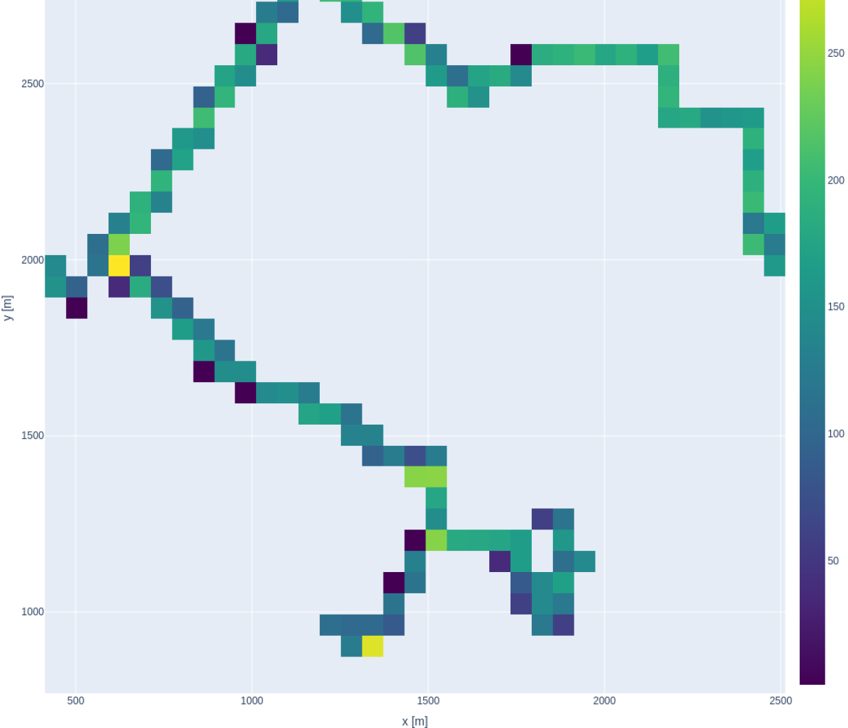
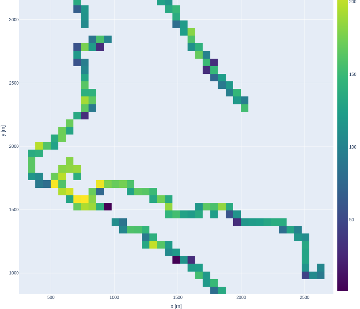
Fig. 10 depicts example images and their position on the map for Boston Seaport. The industrial zones in the south and south-eastern areas have different attributes, e.g. type of buildings, lane widths, number of lanes, and frequency of pedestrian crossings, than the commercial and residential zones in the north-western part. It is thus important that these zones are represented in all sets for a fair evaluation of trained methods. Fig. 11 showcases the regions where samples are allocated in each set for all cities. Each set incorporates regions from different parts of the cities to promote diversity. The heatmaps in Fig. 12 depict the distribution of samples within each 60m cell. One can, for instance, observe a concentration of samples in crossings.

Argoverse 2

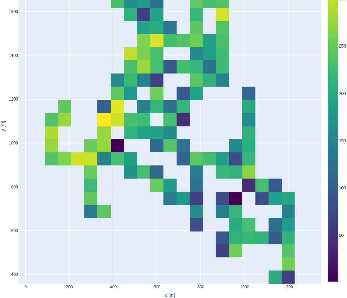
As discussed in Sec. 3.2 it is possible to split Argoverse 2 on a sequence level while preserving zone class diversity. Highlighting the significance of including diverse city areas in all sets, Fig. 13 presents a collection of images from various locations in Washington DC. The downtown area in the southwest exhibits different road characteristics from the sub-urban areas in the north and east. Fig. 14 illustrates how the complete set of city maps are split, ensuring a diverse selection of areas in each set. Heatmaps in Fig. 15 represent the distribution of samples within each 60m cell.

Appendix C Qualitative Results

nuScenes

Fig. 16 portrays three examples with input images, the evaluation prediction, its ground truth, and the closest training sample. Despite not being captured from the exact same pose, these instances demonstrate striking similarities between the evaluation and closest training pose. This underscores that the method, having encountered the closest training sample during training, can achieve accurate predictions through the memorization and retrieval of these examples at test time. Additional examples can be seen in the videos to be part of the project webpage.

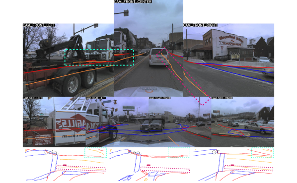
By comparing the predictions of a sample included in the test set for a method trained on both the original and geographical splits, alongside the ground truth, Fig. 17 demonstrates dividers, boundaries, and pedestrian crossings occluded by vehicles in the opposing lane are accurately predicted when the model is trained on the original split. Additionally, the model trained on geographically split data, in contrast to the method trained on original data, identifies the dividers near the ego vehicle. These dividers are visible in the images, but absent in the ground truth, making it tempting to speculate that the method has memorized this information.

Argoverse 2

In Fig. 18, we present three examples featuring input images, the evaluation prediction, its ground truth, and the closest training sample. While not being from the exact same pose, e.g. in the top example the closest training pose is slightly rotated, and in the bottom from an adjacent lane, it is still plausible for a method to achieve a high score on the test sample by memorizing the map and images from the training sample, and then recall and slightly shift and rotate that map at test time. Additional examples will be available on the project webpage.

Fig. 19 illustrate comparisons between predictions derived from a sample included in both the original and geographical splits’ test set, along with the ground truth. Despite the inherent difficulty in predicting objects situated behind a truck on the left side, the model trained on the original split demonstrates commendable accuracy in its estimations. The model also effectively predicts the lane divider to the right of the ego vehicle, when not visibly present in the image but existing in the ground truth. It is worth noting that this may not be due to memorization, as the model could learn, e.g., consistent data annotations and hints from road dividers and road width to accurately predict this non-visible lane divider.