Debiased Machine Learning and Network Cohesion for Doubly-Robust Differential Reward Models in Contextual Bandits

Abstract

A common approach to learning mobile health (mHealth) intervention policies is linear Thompson sampling. Two desirable mHealth policy features are (1) pooling information across individuals and time and (2) incorporating a time-varying baseline reward. Previous approaches pooled information across individuals but not time, failing to capture trends in treatment effects over time. In addition, these approaches did not explicitly model the baseline reward, which limited the ability to precisely estimate the parameters in the differential reward model. In this paper, we propose a novel Thompson sampling algorithm, termed “DML-TS-NNR” that leverages (1) nearest-neighbors to efficiently pool information on the differential reward function across users and time and (2) the Double Machine Learning (DML) framework to explicitly model baseline rewards and stay agnostic to the supervised learning algorithms used. By explicitly modeling baseline rewards, we obtain smaller confidence sets for the differential reward parameters. We offer theoretical guarantees on the pseudo-regret, which are supported by empirical results. Importantly, the DML-TS-NNR algorithm demonstrates robustness to potential misspecifications in the baseline reward model.

1 Introduction

Mobile health (mHealth) and contextual bandit algorithms share a connection in the realm of personalized healthcare interventions. mHealth leverages mobile devices to deliver health-related services for real-time monitoring and intervention. Contextual bandit algorithms, on the other hand, are a class of machine learning techniques designed to optimize decision-making in situations where actions have contextual dependencies. The synergy arises when mHealth applications deploy contextual bandit algorithms to tailor interventions based on individual health data and context. For example, in a mobile health setting, a contextual bandit algorithm might dynamically adapt the type and timing of health-related notifications or interventions based on the user’s current health status, historical behavior, and contextual factors like location or time of day Tewari & Murphy (2017).

At each decision point, a learner receives a context, chooses an action, and observes a reward. The goal is to maximize the expected cumulative reward. High-quality bandit algorithms achieve rewards comparable to those of an optimal policy. To achieve near-optimal performance in mHealth, bandit algorithms must account for (1) the time-varying nature of the outcome variable, (2) nonlinear relationships between states and outcomes, (3) the potential for intervention efficacy to change over time (due, for instance, to habituation as in  Psihogios et al. (2019)), and (4) the fact that similar participants tend to respond similarly to interventions (Künzler et al., 2019).

Traditional mHealth intervention development—including just-in-time adaptive interventions (JITAIs), which aim to tailor the timing and content of notifications to maximize treatment effect (Nahum-Shani et al., 2018)—has centered on treatment policies pre-defined at baseline (e.g., Battalio et al. (2021), Nahum-Shani et al. (2021), Bidargaddi et al. (2018), Klasnja et al. (2019)). As the development of JITAIs shifts towards online learning (e.g., Trella et al. (2022), Liao et al. (2020), Aguilera et al. (2020)), we have the opportunity to incorporate the four key characteristics listed above into the development of optimal treatment policies through algorithms such as contextual bandits.

Although some solutions to these problems have been presented, no existing method offers a comprehensive solution that simultaneously addresses all four challenges in a satisfactory manner. The purpose of this paper is to fill this gap with a method that performs well in the mHealth setting where data is high-dimensional, highly structured, and often exhibits complex nonlinear relationships. To that end, this paper offers three main contributions: (1) A novel algorithm, termed as “DML-TS-NNR” that flexibly models the baseline reward via the double machine learning (DML) framework and pools efficiently across both users and time via nearest-neighbor regularization; (2) theoretical results showing that DML-TS-NNR achieves reduced confidence set sizes and an improved regret bound relative to existing methods; and (3) empirical analysis demonstrating the superior performance of DML-TS-NNR relative to existing methods in simulation and two recent mHealth studies.

The paper proceeds as follows. Section 2 summarizes related work. Section 3 describes the model and problem statement. Section 4 describes the algorithm along with the resulting theoretical results. Section 5 describes experimental results for simulations and two mHealth studies. Section 6 concludes with a discussion of limitations and future work.

2 Related Work

The closest works are Choi et al. (2022) and Tomkins et al. (2021). Choi et al. (2022) employs a semi-parametric reward model for individual users and a penalty term based on the random-walk normalized graph Laplacian. However, limited information is provided regarding the explicit estimation of baseline rewards and the pooling of information across time. In contrast, Tomkins et al. (2021) carefully handles the issue of pooling information across users and time in longitudinal settings, but their approach (intelligentpooling) requires the baseline rewards to be linear and does not leverage network information. Below, we provide a summary of other relevant work in this area.

Thompson Sampling. Abeille & Lazaric (2017) showed that Thompson Sampling (TS) can be posed as a generic randomized algorithm constructed on the regularized least-squares (RLS) estimate rather than one sampling from a Bayesian posterior. At each step $t$, TS samples a perturbed parameter, where the additive perturbation is distributed so that TS explores enough (anti-concentration) but not too much (concentration). Any distribution satisfying these two conditions introduces the right amount of randomness to achieve the desired regret without actually satisfying any Bayesian assumption. We use the high-level proof strategy of Abeille & Lazaric (2017) in this work to derive our regret bound, although we need additional tools to handle our longitudinal setting with baseline rewards.

Partially-linear bandits. Greenewald et al. (2017) introduced a linear contextual bandit with a time-varying baseline and a TS algorithm with $\tilde{O}(d^{2}\sqrt{T})$ regret, where they used the inverse propensity-weighted observed reward as a pseudo-reward. By explicitly modeling the baseline, we obtain a pseudo-reward with lower variance. Krishnamurthy et al. (2018) improved this to $\tilde{O}(d\sqrt{T})$ regret using a centered RLS estimator, eliminating sub-optimal actions, and choosing a feasible distribution over actions. Kim & Paik (2019) proposed a less restrictive, easier to implement, and faster algorithm with a tight regret upper bound. Our regret bound (see Section 4) involves similar rates but is based on a different asymptotic regime that is not directly comparable due to the presence of an increasing pool of individuals.

Nonlinear bandits. (Li et al., 2017, Wang et al., 2019, Kveton et al., 2020) discussed generalized linear contextual bandit algorithms that accommodate nonlinear relationships via parametric link functions in a similar fashion to generalized linear models Nelder & Wedderburn (1972), McCullagh (2019). Other work (e.g., Snoek et al. (2015), Riquelme et al. (2018), Zhang et al. (2019), Wang & Zhou (2020)) allowed non-parametric relationships in both the baseline reward model and advantage function via deep neural networks; however, these approaches typically lack strong theoretical guarantees and are not designed for longitudinal settings in which pooling offers substantial benefit.

Graph bandits. In the study conducted by Cesa-Bianchi et al. (2013), individual-specific linear models were employed, accompanied by a combinatorial Laplacian penalty to encourage similarity among users’ learned models. This approach yielded a regret bound of $\tilde{O}(nd\sqrt{T})$. Building upon this work, Yang et al. (2020) made further improvements by utilizing a penalty involving the random walk graph Laplacian. Their approach offers the following benefits: (1) it achieves a regret bound of $\tilde{O}(\Psi d\sqrt{nT})$ for some $\Psi\in(0,1)$ and (2) it reduces computational complexity from quadratic to linear by utilizing a first-order approximation to matrix inversion.

Double Machine Learning. Chernozhukov et al. (2018) introduced the DML framework, which provides a general approach to obtain $\sqrt{n}$-consistency for a low-dimensional parameter of interest in the presence of a high-dimensional or “highly complex” nuisance parameter. This framework combines Neyman orthogonality and cross-fitting techniques, ensuring that the estimator is insensitive to the regularization bias produced by the machine learning model. Moreover, it allows us to stay agnostic towards the specific machine learning algorithm while considering the asymptotic properties of the estimator. Later, a number of meta-learner algorithms were developed to leverage the DML framework and provide more precise and robust estimators (Hill, 2011, Semenova & Chernozhukov, 2021, Künzel et al., 2019, Nie & Wager, 2021, Kennedy, 2020).

Doubly Robust Bandits. Kim et al. (2021; 2023) use doubly robust estimators for contextual bandits in both the linear and generalized linear settings, respectively. They use them to obtain a novel regret bound with improved dependence on the dimensionality. In our setting, we use a doubly robust pseudo-reward (robust to either the propensity weights or the mean reward estimate being incorrect) in order to debias explicitly modeling the mean reward. We leave combining our approach with theirs for improved dependence on the dimensionality as future work.

3 Model and Problem Statement

We consider a doubly-indexed contextual bandit with a control action ($a=0$) and $K$ non-baseline arms corresponding to different actions or treatments. Individuals $i=1,2,\ldots$ enter sequentially with each individual observed at a sequence of decision points $t=1,2,\ldots$. For each individual $i$ at time $t$, a context vector $S_{i,t}\in\mathcal{S}$ is observed, an action $A_{i,t}\in\{0,\ldots,K\}:=[K]$ is chosen, and a reward $R_{i,t}\in\mathbb{R}$ is observed. In this paper, we assume the conditional model for the observed reward given state and action, i.e., $\mathbb{E}\left[R_{i,t}|S_{i,t}=s,A_{i,t}=a\right]:=r_{i,t}(s,a)$, is given by

$$\begin{split}r_{i,t}(s,a)&=\boldsymbol{x}(s,a)^{\top}\theta_{i,t}\delta_{a>0}+g_{t}(s),\end{split}$$ (1)

where $\boldsymbol{x}(s,a)\in\mathbb{R}^{p\times 1}$ is a vector of features of the state and action, $\delta_{a>0}$ is an indicator that takes value $1$ if $a>0$ and $0$ otherwise, and $g_{t}(s)$ is a baseline reward that is observed when individuals are randomized to not receive any treatment. This can be an arbitrary, potentially nonlinear function of state $s$ and time $t$. Equation (1) is equivalent to assuming a linear differential reward for any $a>0$; i.e., $\Delta_{i,t}(s,a):=r_{i,t}(s,a)-r_{i,t}(s,0)$ is linear in $\boldsymbol{x}(s,a)$, whose parameter $\theta_{i,t}\in\mathbb{R}^{p}$ is allowed to depend both on the individual $i$ and time $t$.

To mimic real-world recruitment where individuals may not enter a study all at once, we consider a study that proceeds in stages. Figure 3 in Appendix A visualizes this sequential recruitment. At stage $1$, the first individual is recruited and observed at time $t=1$. At stage $k$, individuals $j\leq k$ have been observed for $k-j+1$ decision times respectively. Then each individual $j\in[k+1]$ is observed in a random order at their next time step. Let $\mathcal{H}_{i,t}$ denote the observation history up to time $t$ for individual $i$.

We make the following two standard assumptions as in Abeille & Lazaric (2017).

Assumption 1.

The reward is observed with additive error $\epsilon_{i,t}$, conditionally mean 0 (i.e., $\mathbb{E}[\epsilon_{i,t}|\mathcal{H}_{i,t}]=0$) sub-Gaussian with variance $\sigma^{2}$: $\mathbb{E}[\exp(\eta\epsilon_{i,t})|\mathcal{H}_{i,t}]\leq\exp(\eta^{2}\sigma^{2}/2)$ for $\eta>0$.

Assumption 2.

We assume $\|\boldsymbol{x}(s,a)\|\leq 1$ for all contexts and actions and that there exists $B\in\mathbb{R}^{+}$ such that $\|\theta_{i,t}\|\leq B$, $\forall i,t$ and $|g_{t}(s)|\leq B\ \forall s,t$ and $B$ is known.

Here we consider stochastic policies $\pi_{i,t}:\mathcal{H}_{i,t}\times\mathcal{S}\to\mathcal{P}([K])$, which map the observed history $\mathcal{H}_{i,t}$ and current context to a distribution over actions $[K]$. Let $\pi_{i,t}(a|s)$ denote the probability of action $a\in[K]$ given current context $s\in\mathcal{S}$ induced by the map $\pi_{i,t}$ for a fixed (implicit) history.

3.1 DML and Doubly Robust Differential Reward

We first consider a single individual $i$ under a time-invariant linear differential reward, so that $\theta_{i,t}=\theta\in\mathbb{R}^{p}$. If the differential reward $\Delta(s_{i,t},a_{i,t})$ was observed, we could apply ridge regression with a linear model of the form $\boldsymbol{x}(s_{i,t},a_{i,t})^{\top}\theta$ and a ridge penalty of $\lambda\|\theta\|_{2}^{2}$. However, the differential reward is unobserved: we instead consider an inverse-probability weighted (IPW) estimator of the differential reward based on the available data:

$$\begin{split}&\mathbb{E}\left[\left(\frac{\delta_{A_{i,t}=\bar{a}}}{1-\pi_{i,t}(0|s)}-\frac{\delta_{A_{i,t}=0}}{\pi_{i,t}(0|s)}\right)R_{i,t}|s_{i,t},\bar{a}_{i,t}\right]=\Delta_{i,t}(s_{i,t},\bar{a}_{i,t})\end{split}$$ (2)

where $\bar{a}_{i,t}\in[K]$ denotes the potential non-baseline arm that may be chosen if the baseline arm is not chosen; i.e., randomization is restricted to be between $A_{i,t}=\bar{a}_{i,t}$ and $0$. Given the probabilities in the denominators are known, the estimator is unbiased and therefore can replace the observed reward in the Thompson sampling framework.

We refer to this $\Delta_{i,t}(s_{i,t},\bar{a}_{i,t})$ as the differential reward. Below, we define a pseudo-reward with the same expectation in reference to pseudo-outcomes from the causal inference literature (Bang & Robins, 2005, Kennedy, 2020). Let $f_{i,t}(s,a)$ be a working model for the true conditional mean $r_{i,t}(s,a)$. Then, following connections to pseudo-outcomes and doubly-robust (DR) estimators (Kennedy, 2020, Shi & Dempsey, 2023), we define the pseudo-reward $\tilde{R}_{i,t}^{f}(s,\bar{a})$ given state $S_{i,t}=s$ and potential arm $\bar{a}$

$$\tilde{R}_{i,t}^{f}(s,\bar{a})\equiv\frac{\left(R_{i,t}-f_{i,t}(s,A_{i,t})\right)}{\delta_{A_{i,t}=\bar{a}}-\pi_{i,t}(0|s)}+\Delta^{f}_{i,t}(s,\bar{a})$$ (3)

where $\Delta_{i,t}^{f}(s,\bar{a})=f_{i,t}(s,\bar{a})-f_{i,t}(s,0)$. Going forward we will often abbreviate using $\tilde{R}_{i,t}^{f}$, with the state and action implied. Equation (3) presents a Doubly Robust estimator for the Differential Reward; i.e., if either $\pi_{i,t}$ or $f_{i,t}$ are correctly specified, (3) is a consistent estimator of the differential reward—so we refer to it as a DR² bandit. See Appendix G.1 for proof of double robustness. The primary advantage of this pseudo-reward is that by including the $f_{i,t}$, it has lower variance than if we simply used the inverse propensity-weighted observed reward as our pseudo-reward, which was done in Greenewald et al. (2017). Lemma 5 and Remark 2 in Appendix G.2 show proofs and discuss why this pseudo-reward lowers variance compared to Greenewald et al. (2017).

After exploring the properties of the pseudo-reward, an important question arises regarding how we can learn the function $f(s,a)$ using observed data. We hereby provide two options, each based on different assumptions. Option 1 utilizes supervised learning methods and cross-fitting to accurately learn the function while avoiding overfitting as demonstrated in Chernozhukov et al. (2018) and Kennedy (2020). Our model (2) admits sample splitting across time under the assumption of additive i.i.d. errors and no delayed or spill-over effects. Such an assumption is plausible in the mHealth setting where we do not expect an adversarial environment.

In the following, we explain sample splitting as a function of time $t$ as we currently consider a single individual $i$. Step 1: Randomly assign each time $t$ to one of $M$-folds. Let $I_{m}(t)\subseteq\{1,\ldots,t\}$ denote the $m$-th fold as assigned up to time $t$ and $I_{m}^{\complement}(t)$ denote its complement. Step 2: For each fold at each time $t$, use any supervised learning algorithm to estimate the working model for $r_{i,t}(s,a)$ denoted $\hat{f}_{i,t}^{(m)}(s,a)$ using $I_{m}^{\complement}$. Step 3: Construct the pseudo-outcomes using (3) and perform weighted, penalized regression estimation by minimizing the loss function:

$$\begin{split}\sum_{m=1}^{M}\sum_{t\in I_{m}(T)}\tilde{\sigma}_{i,t}^{2}&\bigg{(}\tilde{R}_{i,t}^{\hat{f}^{(m)}}-\boldsymbol{x}(s_{i,t},a_{i,t})^{\top}\theta\bigg{)}^{2}\end{split}$$ (4)

with ridge penalty $\lambda\|\theta\|_{2}^{2}$, where $\tilde{\sigma}_{i,t}^{2}=\pi_{i,t}(0|s_{i,t})\cdot(1-\pi_{i,t}(0|s_{i,t}))$. The weights are a consequence of unequal variances due to the use of DR estimators; i.e., $\text{var}(\tilde{R}_{i,t}^{f})$ is inversely proportional to $(\tilde{\sigma}_{i,t}^{2})^{2}$.

We explore an alternative, Option 2, based on recent work that avoids sample splitting via the use of stable estimators Chen et al. (2022). To relax the i.i.d. error assumption to Assumption 1, we only update $f_{i,t}(s,a)$ using observed history data in an online fashion, fixing pseudo-outcomes at each stage based on the current estimate of the nonlinear baseline. See Appendix C for further discussion.

Finally, in order to obtain guarantees for this DML approach, we make the following two assumptions: the first is on the convergence in $L^{2}$ (with expectation over states and actions) of our estimate $f$ to the true mean reward and boundedness of the estimator. Similar assumptions were made in Chen et al. (2022). The second is that the weights are bounded below, which would be a consequence if the probability of taking no action is bounded above and below, an assumption made in Greenewald et al. (2017) .

Assumption 3.

Both $\mathbb{E}_{p(s,\bar{a})}\left[(r_{i,t}(s,\bar{a})-f_{i,t}(s,\bar{a}))^{2}\right]=o_{P}(k^{-1/2})$ and $\mathbb{E}_{p(s)}\left[(r_{i,t}(s,0)-f_{i,t}(s,0))^{2}\right]=o_{P}(k^{-1/2})$. Further, $|\hat{f}_{i,t}|\leq 2B$.

Assumption 4.

There exists $c>0$ such that $\tilde{\sigma}_{i,t}^{2}>c$ for all $i,t$.

3.2 Nearest Neighbor Regularization

Above, we considered a single individual $i$ under a time-invariant linear differential reward function; i.e., $\boldsymbol{x}(s_{i,t},a_{i,t})^{\top}\theta$ where $\theta\in\mathbb{R}^{p}$. Here, we consider the setting of $N$ independent individuals and a time-invariant linear differential reward with an individual-specific parameter; i.e., $\theta_{i}\in\mathbb{R}^{p}$. If $\theta_{i}$ were known a priori, then one could construct a network based on $L_{2}$-distances $\{d(i,j):=\|\theta_{i}-\theta_{j}\|_{2}^{2}\}_{j\not=i}$.

Specifically, define a graph $G=(V,E)$ where each user represents a node, e.g., $V:=[N]$, and $(i,j)$ is in the edge set $E$ for the smallest $M\ll N$ distances. The working assumption is that connected users share similar underlying vectors $\theta_{i}$, implying that the rewards received from one user can provide valuable insights into the behavior of other connected users. Mathematically, $(i,j)\in E$ implies that $\|\theta_{i}-\theta_{j}\|$ is small.

We define the Laplacian via the $N\times MN$ incidence matrix $B$. The element $B_{v,e}$ corresponds to the $v$-th vertex (user) and $e$-th edge. Denote the vertices of $e$ as $v_{i}$ and $v_{j}$ with $i>j$. $B_{v,e}$ is then equal to 1 if $v=v_{i}$, -1 if $v=v_{j}$, and 0 otherwise. The Laplacian matrix is then defined as $L=BB^{\top}$. We can then adapt (4) by summing over participants and including a network cohesion penalty similar to Yang et al. (2020):

$$\text{tr}(\Theta^{\top}L\Theta)=\sum_{(i,j)\in E}\|\theta_{i}-\theta_{j}\|_{2}^{2},$$

where $\Theta:=(\theta_{1},\ldots,\theta_{N})^{\top}\in\mathbb{R}^{N\times p}$. The penalty is small when $\theta_{i}$ and $\theta_{j}$ are close for connected users. Following Assumption 2 and the above discussion, we further assume:

Assumption 5.

There exists $D\in\mathbb{R}^{+}$ such that $\|\theta_{i}-\theta_{j}\|_{2}^{2}\leq D$, $\forall i,j$, and $D$ is known.

4 DML Thompson Sampling with Nearest Neighbor Regularization

4.1 Algorithm

Based on Section 3, we can now formally state our proposed DML Thompson Sampling with Nearest Neighbor Regularization (DML-TS-NNR) algorithm. In our study, we adopt a sequential recruitment setting in which individuals’ enrollment occurs in a staggered manner to mimic the recruitment process in real mHealth studies. More specifically, we first observe individual $i=1$ at time $t=1$. Then we observe individuals $i=(1,2)$ at times $t=(2,1)$. After $k$ time steps, we observe individuals $i\in[k]$ at times $(k+1-i,k-i,\ldots,1)$ respectively. We then observe these individuals in a random sequence one at a time before moving to stage $k+1$. Define $\mathcal{O}_{k}=\{(i,t):i\leq k\>\&\>t\leq k+1-i\}$ be the set of observed time points across all individuals at stage $k$. Again see Figure 3 in Appendix A for a visualization.

By performing a joint asymptotic analysis with respect to the total number of individuals ($N$) and time points ($T$), we can relax the assumption of a single time-invariant linear advantage function and allow $\theta_{i,t}\in\mathbb{R}^{p}$ to depend on both the individual $i$ and time $t$. Here, we let $\theta_{i,t}=\theta+\theta_{i}^{\textrm{ind}}+\theta_{t}^{\textrm{time}}$; i.e., we include (i) an individual-specific, time-invariant term $\theta_{i}$, and (ii) a shared, time-specific term $\theta_{t}$. This setup is similar to the intelligentpooling method of Tomkins et al. (2021); however, rather than assume individuals and time points are unrelated i.i.d. samples, we assume knowledge of some network information (e.g., the similarity of certain individuals or proximity in time) and regularize these parameters accordingly to ensure network cohesion.

The DML-TS-NNR algorithm is shown in Algorithm 1. To see the motivation, consider the following. We first assume that we have access to two nearest neighbor graphs, $G_{\text{user}}$ and $G_{\text{time}}$, where each characterizes proximity in the user- and time-domains, respectively. Then at stage $k$, we estimate all parameters, e.g. $\Theta_{k}=\textrm{vec}[\left(\theta,\theta_{1}^{\textrm{ind}},\ldots,\theta_{k}^{\textrm{ind}},\theta_{1}^{\textrm{time}},\ldots,\theta_{k}^{\textrm{time}}\right)]\in\mathbb{R}^{p(2k+1)}$ , by minimizing the following penalized loss function $L_{k}(\Theta_{k};\lambda,\gamma)$, which is defined as the following expression:

$$\begin{split}&\sum_{(i,t)\in\mathcal{O}_{k}}\tilde{\sigma}_{i,t}^{2}\left(\tilde{R}_{i,t}^{\hat{f}^{(m)}}-\boldsymbol{x}(S_{i,t},A_{i,t})^{\top}(\theta+\theta_{i}^{\textrm{ind}}+\theta_{t}^{\textrm{time}})\right)^{2}+\\ &\gamma\left(\|\theta\|_{2}^{2}+\sum_{i=1}^{k}\|\theta_{i}^{\textrm{ind}}\|_{2}^{2}+\sum_{t=1}^{k}\|\theta_{t}^{\textrm{time}}\|_{2}^{2}\right)+\lambda\left(\text{tr}\left(\Theta_{\text{user}}^{\top}L_{\text{user}}\Theta_{\text{user}}\right)+\text{tr}\left(\Theta_{\text{time}}^{\top}L_{\text{time}}\Theta_{\text{time}}\right)\right),\end{split}$$ (5)

where $\Theta_{\textrm{user}},\Theta_{\textrm{time}}\in\mathbb{R}^{p\times k}$. In comparison to existing methods, the primary novelty in Equation (5) is that (1) the observed outcome $R_{i,t}$ is replaced by a pseudo-outcome $\tilde{R}^{f^{(k)}}_{i,t}$ and (2) the doubly-robust pseudo-outcome leads to a weighted least-squares loss with weights $\tilde{\sigma}_{i,t}^{2}$. The network cohesion penalties and time-specific parameters have been considered elsewhere (Yang et al., 2020, Tomkins et al., 2021), though, not together. For more details regarding Algorithm 1, please refer to Appendix B.

Algorithm 1 DML-TS with Nearest Neighbor Regularization (DML-TS-NNR)

  Input: $\delta$, $\sigma$, $c$, $C$, $m$, $\lambda$, $\gamma$, $L$, $B_{w}$, $D_{w}$

  Set $L_{\otimes}=L\otimes I_{p}$ and $B=k\frac{\lambda}{\sqrt{\gamma}}\left(D_{\text{ind}}+D_{\text{time}}\right)+\sqrt{\gamma n}\left(B_{\text{ind}}+B_{\text{time}}\right)$

  Initialize: $V_{0}=\operatorname{diag}(\gamma I_{p},\lambda L^{\text{ind}}_{\otimes}+\gamma I_{kp},\lambda L^{\text{time}}_{\otimes}+\gamma I_{kp})$ and $b_{0}=\mathbf{0}$

  for $k=1,\ldots,K$  do

     Option 1: Randomly assign $(i,t)\in\mathcal{O}_{k}\backslash\mathcal{O}_{k-1}$ to one of the $M$ partitions

     Observe Context variable $S_{l}=S_{i_{l},k+i_{l}-1}$

     Set $\hat{\Theta}_{k}=V_{k}^{-1}b_{k}$

     Calculate

$$\beta_{k}(\delta)=v_{k}\left[2\log\left(\frac{\det(V_{k})^{1/2}}{\det(V_{0})^{1/2}\delta/2}\right)\right]^{1/2}+B$$

where $v_{k}^{2}$ is defined in Corollary 4

     Generate $\eta_{k}\sim\mathcal{D}^{TS}$ and compute

$$\tilde{\Theta}_{k}=\hat{\Theta}_{k}+\beta_{k}(\delta^{\prime})V_{k}^{-1/2}\eta_{k}$$

     For each $(i,t)\in\mathcal{O}_{k}\backslash\mathcal{O}_{k-1}$ select $A_{i,t}$ that maximizes:

$$\boldsymbol{x}(S_{i,t},a)^{\top}\left(\tilde{\theta}+\tilde{\theta}_{i}^{\text{ind}}+\tilde{\theta}_{t}^{\text{time}}\right)$$

     Observe rewards $R_{i,t}$

     Construct feature $\boldsymbol{x}_{t}=\boldsymbol{x}(S_{t},A_{t})$ and $\phi_{i,t}=\phi(\boldsymbol{x}_{i,t})$

     Option 1: Re-construct predictions for all $\hat{f}^{(m)}$ partitions for $m=1,\ldots,M$ and re-compute all pseudo-outcomes $\tilde{R}_{i,t}^{\hat{f}^{(m)}}$ for all $(i,t)\in\mathcal{O}_{k}$.

     Option 2: Construct predictions for next stage $\hat{f}^{(k)}$ partitions and compute pseudo-outcomes $\tilde{R}_{i,t}^{\hat{f}^{(k)}}$ only for those $(i,t)\in\mathcal{O}_{k}\backslash\mathcal{O}_{k-1}$ .

     Update $V_{k}=V_{k-1}+\sum_{(i,t)\in\mathcal{O}_{k}\backslash\mathcal{O}_{k-1}}\tilde{\sigma}^{2}_{i,t}\phi_{i,t}\phi_{i,t}^{\top}$ and $b_{k}=b_{k-1}+\sum_{(i,t)\in\mathcal{O}_{k}\backslash\mathcal{O}_{k-1}}\tilde{\sigma}_{i,t}^{2}\tilde{R}_{i,t}^{\hat{f}}\phi_{i,t}$

  end for

4.2 Regret Analysis

Given the knowledge of true parameters $\Theta$, the optimal policy is simply to select, at decision time $t$ for individual $i$, the action $a^{*}_{i,t}=\arg\max_{a\in\mathcal{A}}\boldsymbol{x}(S_{i,t},a)^{\top}(\theta+\theta_{i}+\theta_{t})$ given the state variable $S_{i,t}$. This leads us to evaluate the algorithm by comparing it to this optimal policy after each stage. Given both the number of individuals and the number of time points increases per stage, we define stage $k$ regret to be the average across all individuals at stage $k$:

$$\boldsymbol{\operatorname{Regret}}_{K}=\sum_{k=1}^{K}\frac{1}{k}\left\{\sum_{(i,t)\in\mathcal{O}_{k}\backslash\mathcal{O}_{k-1}}\left[\boldsymbol{x}(S_{i,t},a_{i,t}^{*})^{\top}(\theta^{*}+\theta_{i}^{\star}+\theta_{t}^{\star})-\boldsymbol{x}(S_{i,t},A_{i,t})^{\top}(\theta^{*}+\theta_{i}^{\star}+\theta_{t}^{\star})\right]\right\}$$

This regret is a version of pseudo-regret Audibert et al. (2003). Compared to standard regret, the randomness of the pseudo-regret is due to $\{A_{i,t}\}_{t=1}^{\top}$ since the error terms $\{\epsilon_{i,t}\}_{t=1}^{\top}$ are removed in the definition.

Theorem 1.

Under Assumptions 1 and 2, with probability at least $1-\delta$, Algorithm 1’s regret satisfies

$$\left(\beta_{K}(\delta^{\prime})+\gamma_{K}(\delta^{\prime})\left[1+\frac{4}{d}\right]\right)\sqrt{4cH_{K}Kd\log\left(\gamma+\lambda M+\frac{K+1}{8d}\right)-\log\det\left(V_{0}\right)}$$

$$+\frac{4\gamma_{K}(\delta^{\prime})}{d}\sqrt{\frac{8K}{\lambda}\log\left(\frac{4}{\delta}\right)},$$

where $f_{K}=\operatorname{logdet}V_{K}-\operatorname{logdet}V_{0}$, $V_{0}=\lambda L\otimes I_{p}+\gamma I_{np}$, $\delta^{\prime}=\delta/4K$, $\min(\pi(0|s),1-\pi(0|s))>1/c$ and $H_{K}=O(log(K))$ is the harmonic number. $\beta_{K}$ and $\gamma_{K}$ are defined in Appendix G.

Proof of Theorem 1 is in Appendix G. The regret bound is similar to prior work by Abeille & Lazaric (2017); however, our bound differs in three ways: (1) the harmonic number $H_{K}$ enters as an additional cost for considering average regret per stage with the regret being $O(\sqrt{K}\log^{2}(K))$ having an additional $\log(K)$ factor; (2) the bound depends on the dimension of the differential reward model rather than the dimension of the overall model which can significantly improve the regret bound; and (3) the main benefit of our use of DML is in $\beta_{K}(\delta^{\prime})$ and $\gamma_{K}(\delta^{\prime})$, which depend on the rate of convergence of the model $f$ to the true mean differential reward $r$ as discussed in Appendix G.2, which demonstrates the benefits of good models for this term and how it impacts regret.

Note this regret bound is sublinear in the number of stages and scales only with the differential reward complexity $d$, not the complexity of the baseline reward $g$. As the second term scales with $\sqrt{K}$, for large $K$ we can focus on the first term which scales $O\left(\sqrt{c\cdot d\cdot\log^{2}(K)K}\right)$. Prior work scales sublinearly with the number of decision times $T$ as they assume either a single contextual bandit ($n=1$) or a fixed number of individuals $n$. Greenewald et al. (2017) scales as $O(d^{2}\sqrt{T\log(T)})$ while Yang et al. (2020) scale as $O(\sqrt{\tilde{d}nT\log(T)})$ where $\tilde{d}$ is the complexity of the joint baseline and differential reward model. Interestingly, at stage $K$ we see $n=K$ individuals over $n=K$ decision times (with different number of observations per individual); however, we do not see a regret scale with $\sqrt{nT}=K$. Instead, we only receive an extra $\log(K)$ factor reflecting the benefit of pooling on average regret.

There are several technical challenges to this regret bound. First, the confidence ellipsoids $\beta_{k}$ and $\gamma_{k}$ depend on the sub-Gaussian variance factor of the pseudo-reward and need to be derived for the DML pseudo-reward. Second, two results in Abbasi-Yadkori et al. (2011) need to be reproven: the first is Lemma 7, a linear predictor bound that is used as a key step to derive the final regret bound. It requires handling the fact that our regularized least squares estimate now uses our DML pseudo-reward instead of the observed reward. The second, Proposition 1, requires care as we are now doing weighted regularized least squares. The original version used in Abeille & Lazaric (2017) requires an upper bound on the sum of squared feature norms, but applying Abbasi-Yadkori et al. (2011) only gives us an upper bound on the sum of weighted squared norms. In order to derive the needed bound, we use assumption 4 and then apply Abbasi-Yadkori et al. (2011) to obtain our version of their results that has an upper bound that depends on $c>0$, the lower bound on the weights. Finally, the regret bound itself needs to handle the fact that we have stages with multiple individuals (increasing by one) per stage. This leads to a sum over stages and participants within stages of the difference between RLS and TS (and RLS and true) linear predictors. By some manipulation and an application of Cauchy Schwartz, we see a sum of $\frac{1}{k}$ over stages, which leads to the harmonic number, which describes the additional cost of handling multiple participants in a study in stages.

5 Experiments

5.1 Competitor Comparison Simulation

In this section, we test three versions of our proposed method: (1) DML-TS-NNR-BLM: Our algorithm using an ensemble of Bagged Linear Models, (2) DML-TS-NNR-BT: Our algorithm using an ensemble of Bagged stochastic gradient Trees (Gouk et al., 2019, Mastelini et al., 2021), and (3) DML-TS-SU-BT: Same as (2) but treating the data as if it were derived from a Single User.

We implemented these using Option 2 in Algorithm 1, and compared to four related methods: (1) Standard: Standard Thompson sampling for linear contextual bandits, (2) AC: Action-Centered contextual bandit algorithm (Greenewald et al., 2017), (3) IntelPooling: The intelligentpooling method of Tomkins et al. (2021) fixing the variance parameters close to their true values, and (4) Neural-Linear: a method that uses a pre-trained neural network to transform the feature space for the baseline reward (similar to the Neural Linear method of Riquelme et al. (2018), which in turn was inspired by Snoek et al. (2015)). In general, we expect our method to outperform these methods because it is the only one that can (1) efficiently pool across users and time, (2) leverage network information, and (3) accurately model a complex, nonlinear baseline reward.

We compare these seven methods under three settings that we label as Homogeneous Users, Heterogeneous Users, and Nonlinear. The first two settings involve a linear baseline model and time-homogeneous parameters, but they differ in that the users in the second setting have distinct parameters. The third setting is more general and includes a nonlinear baseline, user-specific parameters, and time-specific parameters. Across all three settings, we simulate 125 stages following the staged recruitment regime depicted in Figure 3 in Appendix A, and we repeat the full 125-stage simulation 50 times. Appendix D provides details on the setup and a link to our implementation.

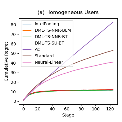
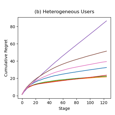
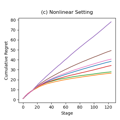
Figure 1: Cumulative regret in the (a) Homogeneous Users, (b) Heterogeneous Users, and (c) Nonlinear settings. The DML methods perform competitively in all three settings and appear to be achieving sublinear regret as expected based on our theoretical results. The DML-TS-NNR-BLM and DML-TS-NNR-BT algorithms perform best, and their final regret is statistically indistinguishable (see Table 1 in Appendix D.2).

Figure 1 shows the cumulative regret for each method at varying stages. DML methods perform competitively against the benchmark methods in all three settings and achieve sublinear regret as expected based on our theoretical results. Across all settings, the best-performing method is either DML-TS-NNR-BLM or DML-TS-NNR-BT. In the first setting, the difference between our methods and IntelPooling is not statistically meaningful because IntelPooling is properly specified and network information is not relevant. In the other two settings, our methods offer substantial and statistically meaningful improvement over the other methods. Appendices D.2 and D.3 shows detailed pairwise comparisons between methods and an additional simulation study using a rectangular array of data.

5.2 Valentine Results

In parallel with the simulation study, we conducted a comparative analysis on a subset of participants from the Valentine Study (Jeganathan et al., 2022), a prospective, randomized-controlled, remotely-administered trial designed to evaluate an mHealth intervention to supplement cardiac rehabilitation for low- and moderate-risk patients. In the analyzed subset, participants were randomized to receive or not receive contextually tailored notifications promoting low-level physical activity and exercise throughout the day. The six algorithms being compared include (1) Standard, (2) AC, (3) IntelPooling, (4) Neural-Linear, (5) DML-TS-SU-RF (RF stands for Random Forest (Breiman, 2001)), and (6) DML-TS-NNR-RF. Figure 2 shows the estimated improvement in average reward over the original constant randomization, averaged over stages (K = 120) and participants (N=108).

To demonstrate the advantage of our proposed algorithm in terms of average reward compared to the competing algorithms, we conducted a pairwise paired t-test with a one-sided alternative hypothesis. The null hypothesis ($H_{0}$) stated that two algorithms achieve the same average reward, while the alternative hypothesis ($H_{1}$) suggested that the column-indexed algorithm achieves a higher average reward than the row-indexed algorithm. Figure 2 displays the p-values obtained from these pairwise t-tests. Since the alternative hypothesis is one-sided, the resulting heatmap is not symmetric. More details on implementation can be found in Appendix E.

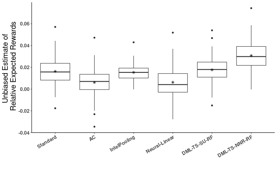
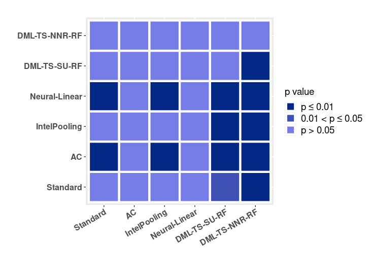
Figure 2: (left) Boxplot of unbiased estimates of the average per-trial reward for all six competing algorithms, relative to the reward obtained under the pre-specified Valentine randomization policy across 100 bootstrap samples. Within each box, the asterisk ($\ast$) indicates the mean value, while the mid-bar represents the median. (right) Heatmap of p-values from the pairwise paired t-tests. The last column’s dark shade indicates that the proposed DML-TS-NNR-RF algorithm achieves significantly higher rewards than the other five competing algorithms. This implies that after implementing our proposed algorithm, the step counts increased by $3.5\%$ more than what the constant randomization policy achieved.

To further enhance the competitive performance of our proposed DML-TS-NNR algorithm, we conducted an additional comparative analysis using a real-world dataset from the Intern Health Study (IHS) (NeCamp et al., 2020). Further details regarding the analysis can be found in Appendix F.

6 Discussion and Future Work

In this paper, we have presented the DML Thompson Sampling with Nearest Neighbor Regularization (DML-TS-NNR) algorithm, a novel contextual bandit algorithm specifically tailored to the mHealth setting. By leveraging the DML framework and network cohesion penalties, DML-TS-NNR is able to accurately model complex, nonlinear baseline rewards and efficiently pool across both individuals and time. The end result is increased statistical precision and, consequently, the ability to learn effective, contextually-tailored mHealth intervention policies at an accelerated pace.

While DML-TS-NNR achieves superior performance relative to existing methods, we see several avenues for improvement. First, the algorithm considers only immediate rewards and, as such, may not adequately address the issue of treatment fatigue. Second, the current algorithm involves computing a log-determinant and matrix inverse, which can be computationally expensive for large matrices. Third, we have made the simplifying assumption that the differential reward is linear in the context vectors. Fourth, we have assumed that the network structure is known and contains only binary edges. Fifth, our algorithm involves several hyperparameters whose values may be difficult to specify in advance. Future work will aim to address these practical challenges in applied settings.

[sections] [sections]l1

Appendix A Recruitment Regime Illustration

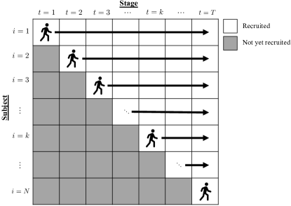
Figure 3: Illustration of the staged recruitment scheme. At each recruitment stage (each time point), a new participant is recruited and observed; at the same time, all participants who were recruited prior to the current stage are also observed again. Observations are not collected from participants who have yet to be recruited. For simplicity, we assume one participant is recruited at each stage.

Appendix B Additional Details for Algorithm 1

The inclusion of $\gamma>0$ ensures a unique solution at each step, while $\lambda$ controls smoothness across the individual-specific and time-specific parameters. In particular, when $\lambda=0$, no information is shared across individuals or across time. A positive value of $\lambda$ introduces the smoothness of these estimates, e.g., if $(i,j)\subset E_{\text{ind}}$ then $\|\theta_{i}^{\text{ind}}-\theta_{j}^{\text{ind}}\|_{2}$ tends to be small. It can be shown that $\sum_{(i,j)\subset E_{\text{ind}}}\|\theta_{i}^{\text{ind}}-\theta_{j}^{\text{ind}}\|_{2}^{2}=\theta_{\text{ind}}^{\top}L_{\otimes}\theta_{\text{ind}}$, where $L_{\otimes}=L\otimes I_{p}$ and $\theta_{\text{ind}}=(\theta_{1}^{\text{ind}},\ldots,\theta_{k}^{\text{ind}})$ is the vector of individual-specific parameters. Let $\boldsymbol{x}_{i,t}:=\boldsymbol{x}(S_{i,t},A_{i,t})$ and $V_{0}=\operatorname{diag}(\gamma I_{p},\lambda L^{\text{ind}}_{\otimes}+\gamma I_{kp},\lambda L^{\text{time}}_{\otimes}+\gamma I_{kp})$. Let $\Phi_{k}$ be the design matrix of features $\phi(\textbf{x}_{i,t})$, $W_{k}$ be the diagonal matrix of weights $\tilde{\sigma}_{i,t}^{2}$, and $R_{k}$ the vector of pseudo-rewards $\tilde{R}_{i,t}^{f^{(k)}}$. In all of these $(i,t)\in\mathcal{O}_{k}$. Then the minimizer $\hat{\Theta}_{k}$ of (5) is

$$[\Phi_{k}^{\top}W_{k}\Phi_{k}+V_{0}]^{-1}[\Phi^{\top}_{k}W_{k}R_{k}] =\underbrace{\Big{[}\sum_{(i,t)\in\mathcal{O}_{k}}\tilde{\sigma}_{i,t}^{2}\phi(\boldsymbol{x}_{i,t})\phi(\boldsymbol{x}_{i,t})^{\top}+V_{0}\Big{]}^{-1}}_{V_{k-1}^{-1}}\underbrace{\Big{[}\sum_{(i,t)\in\mathcal{O}_{k}}\tilde{\sigma}^{2}_{i,t}\tilde{R}_{i,t}^{f^{(k)}}\phi(\boldsymbol{x}_{i,t})\Big{]}}_{b_{k-1}}.$$

where $\phi(\boldsymbol{x}_{i,t})\in\mathbb{R}^{p(2k+1)}$ for any $(i,t)\in\mathcal{O}_{k}$ is defined as

$$\begin{split}\phi(\boldsymbol{x}_{i,t})=(\boldsymbol{x}_{i,t},&\bar{\bf 0}_{(i-1)p},\boldsymbol{x}_{i,t},\bar{\bf 0}_{(k-i)p},\bar{\bf 0}_{(t-1)p},\boldsymbol{x}_{i,t},\bar{\bf 0}_{(k-t)p}).\end{split}$$

The first location of non-zero entries is for the global parameters, the second for the individual parameters and the third for the time parameters.

Remark 1 (Computationally efficient estimation).

Direct calculation of $\hat{\Theta}_{k}$ leads to a computationally expensive inversion of the $(2k+1)\cdot p$ dimensional matrix $V_{t-1}$ at each stage $k$. To avoid this, we observe $V_{k}=V_{k-1}+\sum_{(i,t)\in\mathcal{O}_{k}\backslash\mathcal{O}_{k-1}}\tilde{\sigma}_{i,t}^{2}\phi(\boldsymbol{x}_{i,t})\phi(\boldsymbol{x}_{i,t})^{\top}$ and apply the Sherman-Morrison formula for more efficient computation.

Next, we consider a generic randomized algorithm based on the RLS estimate by sampling a perturbed parameter $\tilde{\Theta}_{k}$ and then selecting an action by simply maximizing the linear differential reward $\boldsymbol{x}(s,a)^{\top}(\tilde{\theta}+\tilde{\theta}_{i}+\tilde{\theta}_{t})$. This construction includes standard Thompson sampling as an important special case. Specifically, we construct $\tilde{\Theta}_{k}=\hat{\Theta}_{k}+\beta_{k}(\delta^{\prime})V_{k}^{-1/2}\eta_{k}$ where $\eta_{k}$ is a random sample drawn i.i.d. from a suitable multivariate distribution $\mathcal{D}^{\text{TS}}$ and $\beta_{k}(\delta^{\prime})$ is a term from the self-normalization bound (Theorem 2) developed in Abbasi-Yadkori et al. (2011). Because of our use of $f_{i,t}$ to approximate $r_{i,t}$, $\beta_{k}(\delta^{\prime})$ is smaller, and thus our distribution for $\hat{\Theta}_{k}$ has lower variance than if we did not use $f_{i,t}$. We discuss this in detail in Appendix G.2. To ensure small regret, we must choose the random variable $\eta_{k}$ to ensure sufficient exploration but not too much. Definition 1 is from Abeille & Lazaric (2017) and formalizes the properties of the random variable $\eta_{k}$.

Definition 1.

$\mathcal{D}^{TS}$ is a multivariate distribution on $\mathbb{R}^{d}$ absolutely continuous with respect to Lebesgue measure which satisfies: 1. (anti-concentration) that there exists a strictly positive probability $p$ such that for any $u\in\mathbb{R}^{d}$ with $\|u\|=1$, $\mathbb{P}(u^{\top}\eta\geq 1)\geq p$; and 2. (concentration) there exists $c$, $c^{\prime}$ positive constants such that $\forall\delta\in(0,1)$, $P(\|\eta\|\leq\sqrt{cd\log(c^{\prime}d/\delta))}\geq 1-\delta$.

While a Gaussian prior satisfies Definition 1, this approach allows us to move beyond Bayesian posteriors to generic randomized policies. In practice, the true parameter values $\Theta$ are unknown, so $\beta_{k}(\delta^{\prime})$ is not available. Thus one needs to insert upper bounds for $\|\mathcal{L}^{\text{ind}}_{\otimes}\theta_{\text{ind}}\|_{2}$ and $\|\theta_{\text{ind}}\|_{2}$ and similarly for time-specific parameters. For example, $\|L_{\otimes}\theta\|_{2}\leq M\cdot N\max_{(i,j)\in E}\|\theta_{i}-\theta_{j}\|_{2}$. Similarly, based on $\|\theta\|_{2}\leq\sqrt{k}\max_{i}\|\theta_{i}\|_{2}$, by Assumption 2, we have $\|\theta\|_{2}\leq\sqrt{k}B$.

Appendix C Option 1 & 2

In Algorithm 1, we provide two options for constructing $\hat{f}$ and the corresponding pseudo-outcomes $\tilde{R}_{i,t}^{\hat{f}}$. Option 1 assumes i.i.d. additive error and recomputes the pseudo-rewards, $\tilde{R}_{i,t}^{\hat{f}^{(m)}}$, at each stage for all $i,t$ using an updated estimate of $f$, which can be estimated using either (a) sample splitting or (b) stable estimators, such as bagged ensembles constructed via sub-sampling. Option 2 uses historical data to generate predictions in an online fashion, and calculates the pseudo-rewards only once without updating them for all subsequent stages.

Our simulations have confirmed that both options result in comparable regret. In reality, however, it’s important to note that the decisions made for individual $i$ at time $t$ may depend on all previous data. Based on this argument, Option 2 was used in both case studies and simulations, highlighting the benefits of our approach in numerical as well as real-world mHealth studies, as detailed in the manuscript.

C.1 Option 1

Sample splitting has been widely used in the DML-related literature (Chernozhukov et al., 2018, Kennedy, 2020) to relax modeling constraints in constructing $\hat{f}$. This approach allows the flexibility of the model to increase with the sample size while protecting against overfitting. As a result, complex machine learning algorithms can be utilized to estimate the function $f$, resulting in accurate estimation of the differential reward $\Delta^{f}$ and, consequently, precise estimates of the $\theta$’s in the linear differential reward function.

When implemented as part of our proposed algorithm, sample splitting randomly partitions all available data into $M$ folds. This step relies heavily on the assumption of i.i.d additive errors, as the random splits are formed on a per-observation basis. Theoretical findings outlined in Chernozhukov et al. (2018) demonstrate the crucial role of sample splitting in achieving $\sqrt{n}$-consistency and ensuring the validity of inferential statements for the parameters in the linear differential reward function.

As an alternative to sample splitting, one can instead construct $\hat{f}$ via stable estimators that exhibit a $o(n^{-1/2})$ leave-one-out stability. A recent study by Chen et al. (2022) demonstrated that estimators based on predictive models that satisfy this condition can achieve $\sqrt{n}$-consistency and asymptotic normality without relying on the Donsker property or employing sample splitting.

The stability conditions outlined in Theorem 5 of Chen et al. (2022) are satisfied by bagging estimators formed with sub-sampling. We leverage this result in Section 5 by testing several versions of our method based on bagged estimators: two based on bagged stochastic gradient trees (DML-TS-NNR-BT and DML-TS-SU-BT) and one based on bagged linear models (DML-TS-NNR-BLM).

As long as the errors are i.i.d., methods based on either (a) sample splitting or (b) stable estimators are permissible within our method. In both cases, we are able to leverage both current and previous observations to construct the latest estimation of $\hat{f}$.

C.2 Option 2

In the mobile health setting, deviations from the expected reward typically represent the effects of idiosyncratic error as opposed to adversarial actions. Consequently, the i.i.d. assumption is more plausible in mobile health than in general contextual bandit settings. However, due to the sequential design of mobile health studies, one challenge that may arise is dependence across time within individual users. Option 2 adapts our method to address this challenge.

When considering errors that exhibit temporal dependence, it is reasonable to utilize past observations to create future pseudo-rewards but not the other way around. For instance, at stage $k$, we train the model $\hat{f}^{(k)}$ using all the history observed up until stage $k-1$ and construct pseudo-rewards for the rewards observed in stage $k$; however, we do not use $\hat{f}^{(k)}$ to update pseudo-rewards for previous stages.

Fixing the pseudo-rewards in this manner enables us to move beyond the assumption of i.i.d. additive errors. This approach is compatible with both the sample splitting and bagging approaches discussed previously. As a computational convenience, researchers may choose to update $\hat{f}$ in an online fashion as we did in Section 5.1. The primary tradeoff in doing so is that the online predictive model may not perform as well as a model trained in one batch, especially in the early stages.

Appendix D Additional Details for Simulation Study

The code for the simulation study is fully containerized and publicly available at https://redacted/for/anonymous/peer/review.

D.1 Setup Details

We consider a generative model of the following form for user $i$ at time $t$:

$$R_{it}=g(S_{it})+x(S_{it},A_{it})\,\theta_{it}+\epsilon_{it},\quad\epsilon_{it}\sim\mathcal{N}(0,1)$$

Here $S_{it}=(s_{1},s_{2})\in\mathbb{R}^{2}$ is a context vector, with both dimensions $\overset{iid}{\sim}U(-1,1)$. We set $x(s,a)=a\,(1,s_{1},s_{2})$. For simplicity, we set $g$ to a time-homogeneous function. The specific nature of the function varies across the following three settings mentioned in Section 5.1:

• Homogeneous Users: Standard contextual bandit assumptions with a linear baseline and no user- or time-specific parameters. The linear baseline is $g(S_{it})=2-2s_{1}+3s_{2}$, and the causal parameter is $\theta_{it}=(1,0.5,-4)$ such that the optimal action varies across the state space.

• Heterogeneous Users: Same as the above but each user’s causal parameter has iid $\mathcal{N}(0,1)$ noise added to it.

• Nonlinear: The general setting discussed in the paper with a nonlinear baseline, user-specific parameters, and time-specific parameters. The base causal parameter and user-specific parameters are the same as in the previous two settings. The nonlinear baseline and time-specific parameter are shown in Figure 4.

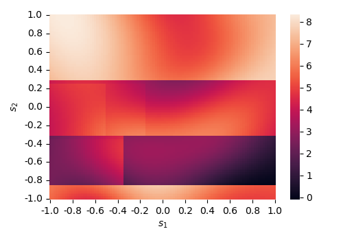
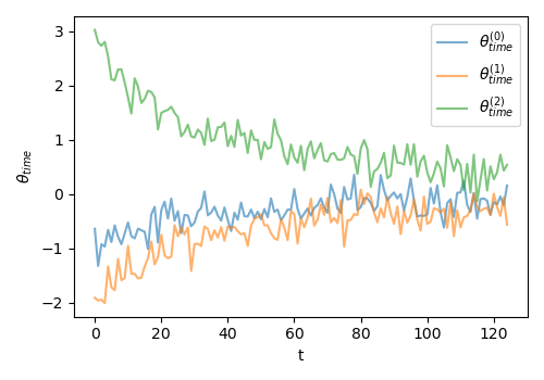
Figure 4: (left) The baseline reward function $g(S_{it})$ used in the simulation study. The proposed method allows this function to be a nonlinear function of the context vectors. The baseline was generated using a combination of recursive partitioning and by summing scaled, shifted, and rotated Gaussian densities. (right) The time-specific parameters used in the simulation study. These parameters cause the advantage function to vary over time. We set them such that the advantage function changes quickly at the beginning of the study then stabilizes.

We assume that the data are observed via a staged recruitment scheme, as illustrated in Figure 3 in Appendix A. For computational convenience, we update parameters and select actions in batches. If, for instance, we observe twenty users at a given stage, we update our estimates of the relevant causal parameters and select actions for all twenty users simultaneously. This strategy offers a slight computational advantage with limited implications in terms of statistical performance.

For simplicity, we assume that the nearest neighbor network is known and set the relevant hyperparameters accordingly. We took care to set $\gamma$ such that our method performs a similar amount of shrinkage compared to other methods, such as IntelPooling, which effectively uses a separate penalty matrix for users and time. To do so, we set a separate value of $\gamma$ for both users and time and set it to the maximum eigenvalue of the penalty matrix (random effect precision matrix) used by IntelPooling. We use 5 neighbors within the DML methods and set the other hyperparameters as follows: $\sigma=1$, $\lambda=1$, and $\delta=0.01$.

For the Neural-Linear method, we generate a $125\times 125$ array of baseline rewards (no action-specific component) to train the neural network prior to running the bandit algorithm. Consequently, the results shown in the paper for Neural-Linear are better than would be observed in practice because we allowed the Neural-Linear method to leverage data that we did not make available to the other methods. This setup offers the computational benefit of not needing to update the neural network within bandit replications, which substantially reduces the necessary computation time.

Aside from the input features used, the Neural-Linear method has the same implementation as the Standard method. The Neural-Linear method uses the output from the last hidden layer of a neural network to model the baseline reward. However, we use the original features (the state vectors) to model the advantage function because the true advantage function is, in fact, linear in these features.

Our neural networks consisted of four hidden layers with 10, 20, 20, and 10 nodes, respectively. The first two employ the ReLU activation function (Nair & Hinton, 2010) while the latter two employ the hyperbolic tangent. We chose to use the hyperbolic tangent for the last two layers because Snoek et al. (2015) found that smooth activation functions such as the hyperbolic tangent were advantageous in their neural bandit algorithm. The loss function was the mean squared error between the neural networks’ output and the baseline reward on a simulated data set. We trained our networks using the Adam optimizer (Kingma & Ba, 2014) with batch sizes of 200 for between 20 and 50 epochs. We simulated a separate validation data set to ensure to check that our model had converged and was generating accurate predictions.

Figure 5 compares the true baseline reward function in the nonlinear setting (left) to that estimated by the neural network (right). We see that neural network produced an accurate approximation of the baseline reward, which helps explain the good performance of the Neural-Linear method relative to other baseline approaches, such as Standard.

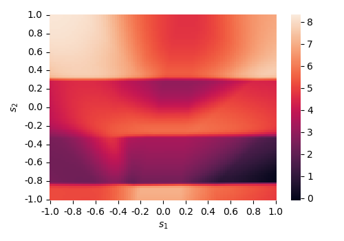
Figure 5: (left) The baseline reward function $g(S_{it})$ used in the simulation study compared to (right) the estimated baseline reward from our neural network in the nonlinear setting.

We include the Neural-Linear method primarily to demonstrate that correctly modeling the baseline is not sufficient to ensure good performance. In the mobile health context, algorithms should also be able to (1) efficiently pool data across users and time and (2) leverage network information. The Neural-Linear method satisfies neither of these criteria. Note that a neural network could be used to model the baseline rewards as part of our algorithm. Future work could consider allowing the differential rewards themselves to also be complex nonlinear functions, which could be accomplished by combining our method with Neural-Linear. We leave the details to future work.

D.2 Pairwise Comparisons for Main Simulation

Table 1 shows pairwise comparisons between methods across the three settings. The individual cells indicate the percentage of repetitions (out of 50) in which the method listed in the row outperformed the method listed in the column. The asterisks indicate p-values below 0.05 from paired two-sided t-tests on the differences in final regret. The Avg column indicates the average pairwise win percentage.

The DML-TS-NNR-BLM and DML-TS-NNR-BT methods perform well across all three settings and the difference between them is statistically indistinguishable. These methods perform about equally well compared to IntelPooling in the first setting, but they perform better in the other settings because the DML methods (1) can leverage network information and (2) can accurately model the nonlinear baseline reward in the third setting.

DML-TS-NNR-BLM and DML-TS-NNR-BT perform especially well in the nonlinear setting, the more general setting for which they were designed. They achieve pairwise win percentages of 91% and 87%, respectively, compared to only 48% for the next-best non-DML method (IntelPooling).

Homogeneous Users

	1	2	3	4	5	6	7	Avg
1. IntelPooling	-	54%	46%	58%	100%*	100%*	100%*	76%
2. DML-TS-NNR-BLM	46%	-	50%	52%	100%*	100%*	100%*	75%
3. DML-TS-NNR-BT	54%	50%	-	58%	100%*	100%*	100%*	77%
4. DML-TS-SU-BT	42%	48%	42%	-	100%*	100%*	100%*	72%
5. AC	0%*	0%*	0%*	0%*	-	0%*	0%*	0%
6. Standard	0%*	0%*	0%*	0%*	100%*	-	0%*	17%
7. Neural-Linear	0%*	0%*	0%*	0%*	100%*	100%*	-	33%

Heterogeneous Users

	1	2	3	4	5	6	7	Avg
1. IntelPooling	-	0%*	10%*	10%*	100%*	100%*	84%*	51%
2. DML-TS-NNR-BLM	100%*	-	54%	66%*	100%*	100%*	100%*	87%
3. DML-TS-NNR-BT	90%*	46%	-	64%	100%*	100%*	100%*	83%
4. DML-TS-SU-BT	90%*	34%*	36%	-	100%*	100%*	100%*	77%
5. AC	0%*	0%*	0%*	0%*	-	0%*	0%*	0%
6. Standard	0%*	0%*	0%*	0%*	100%*	-	0%*	17%
7. Neural-Linear	16%*	0%*	0%*	0%*	100%*	100%*	-	36%

Nonlinear

	1	2	3	4	5	6	7	Avg
1. IntelPooling	-	2%*	6%*	24%*	100%*	94%*	62%*	48%
2. DML-TS-NNR-BLM	98%*	-	56%	94%*	100%*	100%*	100%*	91%
3. DML-TS-NNR-BT	94%*	44%	-	84%*	100%*	100%*	98%*	87%
4. DML-TS-SU-BT	76%*	6%*	16%*	-	100%*	100%*	90%*	65%
5. AC	0%*	0%*	0%*	0%*	-	0%*	0%*	0%
6. Standard	6%*	0%*	0%*	0%*	100%*	-	10%*	19%
7. Neural-Linear	38%*	0%*	2%*	10%*	100%*	90%*	-	40%

Table 1: Pairwise comparisons between methods in the three settings of the main simulation. Each cell indicates the percent of repetitions (out of 50) in which the method listed in the row outperformed the method listed in the column in term of final regret. Asterisks indicate p-values below 0.05 from paired two-sided t-tests on the differences in final regret. The full DML methods (DML-TS-NNR-BLM and DML-TS-NNR-BT) perform best in all three settings and their final regret is statistically indistinguishable.

D.3 Simulation with Rectangular Data Array

The main simulation involves simulating data from a triangular data array. At the 125-th (final) stage, the algorithm has observed 125 rewards for user 1, 124 rewards for user 2, and so on.

In this section, we simulate actions and rewards under a rectangular array with 100 users and 100 time points. Although we still follow the staged recruitment regime depicted in Figure 3 in Appendix A, at stage 100 we stop sampling actions and rewards for user 1; at stage 101 we stop sampling for user 2; and so on until we have sampled 100 time points for all 100 users. Aside from the shape of the data array, the setup is the same for this simulation as for the main simulation.

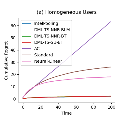
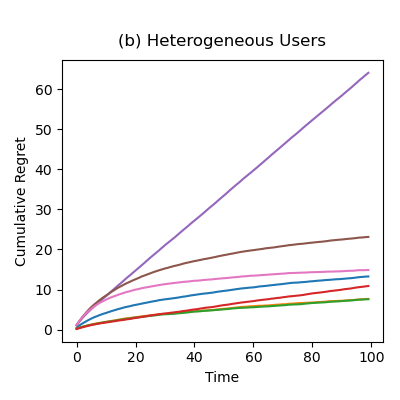
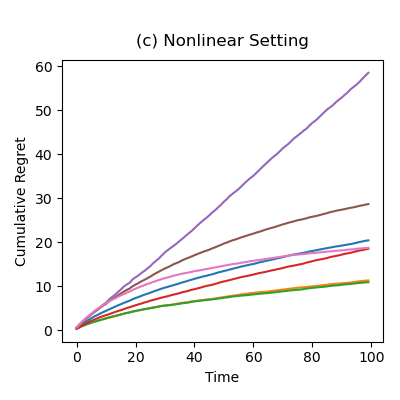
Figure 6: Cumulative regret in the (a) Homogeneous Users, (b) Heterogeneous Users, and (c) Nonlinear settings using a rectangular array of data in which we observe 100 time points for 100 users in a stagewise fashion as depicted in Figure 3 in Appendix A. Similar to Figure 1, the full DML methods (DML-TS-NNR-BLM and DML-TS-NNR-BT) are highly competitive in all three settings and substantially outperform the other methods in the nonlinear setting.

The cumulative regret for these methods as a function of time—not stage—is shown in Figure 6. The qualitative results are quite similar to those from the main simulation. DML-TS-NNR-BLM and DML-TS-NNR-BT are highly competitive in all three scenarios and substantially outperform the other methods in the nonlinear setting; in fact, compared to the main simulation, the improvement of these methods over the others is even larger.

Homogeneous Users

	1	2	3	4	5	6	7	Avg
1. IntelPooling	-	62%	60%	58%	100%*	100%*	100%*	80%
2. DML-TS-NNR-BLM	38%	-	50%	44%	100%*	100%*	100%*	72%
3. DML-TS-NNR-BT	40%	50%	-	44%	100%*	100%*	100%*	72%
4. DML-TS-SU-BT	42%	56%	56%	-	100%*	100%*	100%*	76%
5. AC	0%*	0%*	0%*	0%*	-	0%*	0%*	0%
6. Standard	0%*	0%*	0%*	0%*	100%*	-	0%*	17%
7. Neural-Linear	0%*	0%*	0%*	0%*	100%*	100%*	-	33%

Heterogeneous Users

	1	2	3	4	5	6	7	Avg
1. IntelPooling	-	0%*	0%*	8%*	100%*	100%*	86%*	49%
2. DML-TS-NNR-BLM	100%*	-	48%	100%*	100%*	100%*	100%*	91%
3. DML-TS-NNR-BT	100%*	52%	-	100%*	100%*	100%*	100%*	92%
4. DML-TS-SU-BT	92%*	0%*	0%*	-	100%*	100%*	100%*	65%
5. AC	0%*	0%*	0%*	0%*	-	0%*	0%*	0%
6. Standard	0%*	0%*	0%*	0%*	100%*	-	0%*	17%
7. Neural-Linear	14%*	0%*	0%*	0%*	100%*	100%*	-	36%

Nonlinear

	1	2	3	4	5	6	7	Avg
1. IntelPooling	-	0%*	0%*	12%*	100%*	100%*	18%*	38%
2. DML-TS-NNR-BLM	100%*	-	44%	100%*	100%*	100%*	100%*	91%
3. DML-TS-NNR-BT	100%*	56%	-	100%*	100%*	100%*	100%*	93%
4. DML-TS-SU-BT	88%*	0%*	0%*	-	100%*	100%*	64%	59%
5. AC	0%*	0%*	0%*	0%*	-	0%*	0%*	0%
6. Standard	0%*	0%*	0%*	0%*	100%*	-	0%*	17%
7. Neural-Linear	82%*	0%*	0%*	36%	100%*	100%*	-	53%

Table 2: Pairwise comparisons between methods in the three settings of the simulation with a rectangular array of data. As in Table 1, each cell indicates the percent of repetitions (out of 50) in which the method listed in the row outperformed the method listed in the column in term of final regret. Asterisks indicate p-values below 0.05 from paired two-sided t-tests on the differences in final regret. The full DML methods (DML-TS-NNR-BLM and DML-TS-NNR-BT) perform best in all three settings in terms of pairwise win percentages and are not significantly different from each other.

Table 2 displays the results from pairwise method comparisons, similar to those shown in Table 1. Again the results are qualitatively similar to those from the main simulation. In 26/30 pairwise comparisons, DML-TS-NNR-BLM and DML-TS-NNR-BT outperform the other methods in 100% of replications. The four remaining pairwise comparisons are not statistically significant and result from comparisons with DML-TS-SU-BT and IntelPooling in the “Homogeneous Users” setting. DML-TS-NNR-BLM and DML-TS-NNR-BT offer little or no benefit compared to these methods in that setting because (1) the baseline is linear, (2) no network information is available, (3) no time effects are present, and (4) partial pooling (employed by DML-TS-NNR-BLM, DML-TS-NNR-BT, and IntelPooling) offers no benefit compared to full pooling (employed by DML-TS-SU-BT) because the causal effects are exactly the same among users.

In summary, our methods substantially outperform the other methods in complex, general settings and perform competitively with the other methods in simple settings.

Appendix E Additional Details for Valentine Study

Personalizing treatment delivery in mobile health is a common application for online learning algorithms. We focus here on the Valentine study, a prospective, randomized-controlled, remotely administered trial designed to evaluate an mHealth intervention to supplement cardiac rehabilitation for low- and moderate-risk patients (Jeganathan et al., 2022). We aim to use smart watch data (Apple Watch and Fitbit) obtained from the Valentine study to learn the optimal timing of notification delivery given the users’ current context.

E.1 Data from the Valentine Study

Prior to the start of the trial, baseline data was collected on each of the participants (e.g., age, gender, baseline activity level, and health information). During the study, participants are randomized to either receive a notification ($A_{t}=1$) or not ($A_{t}=0$) at each of 4 daily time points (morning, lunchtime, mid-afternoon, evening), with probability 0.25. Contextual information was collected frequently (e.g., number of messages sent in prior week, step count variability in prior week, and pre-decision point step-counts).

Since the goal of the Valentine study is to increase participants’ activity levels, we thereby define the reward, $R_{t}$, as the step count for the 60 minutes following a decision point (log-transformed to eliminate skew). Our application also uses a subset of the baseline and contextual data; this subset contains the variables with the strongest association to the reward. Table 3 shows the features available to the bandit in the Valentine study data set.

Feature	Description	Interaction	Baseline Model
Phase II	1 if in Phase II, 0 o.w.	$\surd$	$\surd$
Phase III	1 if in Phase II, 0 o.w.	$\surd$	$\surd$
Steps in prior 30 minutes	log transformed	$\surd$	$\surd$
Pre-trial average daily steps	log transformed	$\times$	$\surd$
Device	1 if Fitbit, 0 o.w.	$\times$	$\surd$
Prior week step count variability	SD of the rewards in prior week	$\times$	$\surd$

Table 3: List of features available to the bandit in the Valentine study. The features available to model the action interaction (effect of sending an anti-sedentary message) and to model the baseline (reward under no action) are denoted via a “$\surd$” in the corresponding column, otherwise $\times$.

For baseline variables, we use the participant’s device model ($Z_{1}$, Fitbit coded as 1), the participant’s step count variability in the prior week ($Z_{2}$), and a measure of the participant’s pre-trial activity level based on an intake survey ($Z_{3}$, with larger values corresponding to higher activity levels).

At every decision point, before selecting an action, the learner sees two state variables: the participant’s previous 30-minute step count ($S_{1}$, log-transformed) and the participant’s phase of cardiac rehabilitation ($S_{2}$, dummy coded). The cardiac rehabilitation phase is defined based on a participant’s time in the study: month 1 represents Phase I, month 2-4 represents Phase II, and month 5-6 represents Phase III.

E.2 Evaluation

The Valentine study collected the sensor-based features at 4 decision points per day for each study participant. The reward for each message was defined to be $\text{log}(0.5+x)$, where $x$ is the step count of the participant in the 60 minutes following the notification. As noted in the introduction, the baseline reward, i.e. the step count of a subject when no message is sent, not only depends on the state in a complex way but is likely dependent on a large number of time-varying observed variables. Both these characteristics (complex, time-varying baseline reward function) suggest using our proposed approach.

We generated 100 bootstrap samples and ran our contextual bandit on them, considering the binary action of whether or not to send a message at a given decision point based on the contextual variables $S_{1}$ and $S_{2}$. Each user is considered independently and with a cohesion network, for maximum personalization and independence of results. To guarantee that messages have a positive probability of being sent, we only sample the observations with notification randomization probability between $0.01$ and $0.99$. In the case of the algorithm utilizing NNR, we chose four baseline characteristics (gender, age, device, and baseline average daily steps) to establish a measure of “distance” between users. For this analysis, the value of $k$ representing the number of nearest neighbors was set to 5. To utilize bootstrap sampling, we train the Neural-Linear method’s neural network using out-of-bag samples. The neural network architecture comprises a single hidden layer with two hidden nodes. The input contains both the baseline characteristics and the contextual variables and the activation function applied here is the softplus function, defined as $\text{softplus}(x)=\log(1+\exp{(x)})$.

We performed an offline evaluation of the contextual bandit algorithms using an inverse propensity score (IPS) version of the method from Li et al. (2010), where the sequence of states, actions, and rewards in the data are used to form a near-unbiased estimate of the average expected reward achieved by each algorithm, averaging over all users.

E.3 Inverse Propensity Score (IPS) offline evaluation

In the implemented Valentine study, the treatment was randomized with a constant probability $p_{t}=0.25$ at each time $t$. To conduct off-policy evaluation using our proposed algorithm and the competing variations of the TS algorithm, we outline the IPS estimator for an unbiased estimate of the per-trial expected reward based on what has been studied in Li et al. (2010).

Given the logged data $\mathcal{D}=\{s_{t}=s_{t},A_{t}=a_{t},R_{t}=r_{t}\}_{t=1}^{T}$ collected under the policy $\mathbf{p}=\{p_{t}\}_{t=1}^{T}$, and the treatment policy being evaluated $\mathbf{\pi}=\{\pi_{t}\}_{t=1}^{T}$, the objective of this offline estimator is to reweight the observed reward sequence $\{R_{t}\}_{t=1}^{T}$ to assign varying importance to actions based on the propensities of both the original and new policies in selecting them.

Lemma 1 (Unbiasedness of the IPS estimator).

Assuming the positivity assumption in logging, which states that for any given $s$ and $a$, if $p_{t}(a|s)>0$, then we also have $\pi_{t}(a|s)>0$, we can obtain an unbiased per-trial expected reward using the following IPS estimator:

$$\hat{R}_{\text{IPS}}=\frac{1}{T}\sum_{t=1}^{T}\frac{\pi_{t}(a_{t}|s_{t})}{p_{t}(a_{t}|s_{t})}r_{t}$$ (6)

As mentioned in the previous section, we restrict our sampling to observations with notification randomization probabilities ranging from 0.01 to 0.99. This selection criterion ensures the satisfaction of the positivity assumption. The proof essentially follows from definition, we have:

Proof.

$$\mathbb{E}[R_{\text{IPS}}] =\mathbb{E}_{\mathbf{p}}\left[\frac{1}{T}\sum_{t=1}^{T}\frac{\pi_{t}(a_{t}|s_{t})}{p_{t}(a_{t}|s_{t})}R_{t}(a_{t},s_{t})\right]$$

$$=\frac{1}{T}\sum_{t=1}^{T}\frac{\pi_{t}(a_{t}|s_{t})}{p_{t}(a_{t}|s_{t})}R_{t}(a_{t},s_{t})\times p_{t}(a_{t}|s_{t})$$

$$=\frac{1}{T}\sum_{t=1}^{T}\pi_{t}(a_{t}|s_{t})R_{t}(a_{t},s_{t})$$

$$=\mathbb{E}_{\mathbf{\pi}}\left[\frac{1}{T}\sum_{t=1}^{T}R_{t}(a_{t},s_{t})\right]$$

∎

To address the instability issue caused by re-weighting in some cases, we use a Self-Normalized Inverse Propensity Score (SNIPS) estimator. This estimator scales the results by the empirical mean of the importance weights, and still maintains the property of unbiasedness.

$$\hat{R}_{\text{SNIPS}}=\frac{\hat{R}_{\text{IPS}}}{\frac{1}{T}\sum_{t=1}^{T}\frac{\pi_{t}(a_{t}|s_{t})}{p_{t}(a_{t}|s_{t})}}=\frac{\sum_{t=1}^{T}\frac{\pi_{t}(a_{t}|s_{t})}{p_{t}(a_{t}|s_{t})}r_{t}}{\sum_{t=1}^{T}\frac{\pi_{t}(a_{t}|s_{t})}{p_{t}(a_{t}|s_{t})}}$$ (7)

Appendix F Additional Details for the Intern Health Study (IHS)

To further enhance the competitive performance of our proposed DML-TS-NNR algorithm, we conducted an additional comparative analysis using a real-world dataset from the Intern Health Study (IHS) (NeCamp et al., 2020). This micro-randomized trial investigated the use of mHealth interventions aimed at improving the behavior and mental health of individuals in stressful work environments. The estimates obtained represent the improvement in average reward relative to the original constant randomization, averaging across stages (K = 30) and participants (N = 1553). The available IHS data consist of 20 multiple-imputed data sets. We apply the algorithms to each imputed data set and perform a comparative analysis of the competing algorithms. The results presented in Figure 7 shows our proposed DML-TS-NNR-RF algorithm achieved significantly higher rewards than the other three competing ones and demonstrated comparable performance to the AC algorithm. These findings further support the advantages of our proposed algorithm.

F.1 Data from the IHS

Prior to the start of the trial, baseline data was collected on each of the participants (e.g., institution, specialty, gender, baseline activity level, and health information). During the study, participants are randomized to either receive a notification ($A_{t}=1$) or not ($A_{t}=0$) every day, with probability $3/8$. Contextual information was collected frequently (e.g., step count in prior five days, and current day in study).

We hereby define the reward, $R_{t}$, as the step count on the following day (cubic root). Our application also uses a subset of the baseline and contextual data; this subset contains the variables with the strongest association to the reward. Table 4 shows the features available to the bandit in the IHS data set.

Feature	Description	Interaction	Baseline
Day in study	an integer from $1$ to $30$	$\surd$	$\surd$
Average daily steps in prior five days	cubic root	$\surd$	$\surd$
Average daily sleep in prior five days	cubic root	$\times$	$\surd$
Average daily mood in prior five days	a Likert scale from $1-10$	$\times$	$\surd$
Pre-intern average daily steps	cubic root	$\times$	$\surd$
Pre-intern average daily sleep	cubic root	$\times$	$\surd$
Pre-intern average daily mood	a Likert scale from $1-10$	$\times$	$\surd$
Sex	Gender	$\times$	$\surd$
Week category	The theme of messages in a specific week (mood, sleep, activity, or none)	$\times$	$\surd$
PHQ score	PHQ total score	$\times$	$\surd$
Early family environment	higher score indicates higher level of adverse experience	$\times$	$\surd$
Personal history of depression		$\times$	$\surd$
Neuroticism (Emotional experience)	higher score indicates higher level of neuroticism	$\times$	$\surd$

Table 4: List of features available to the bandit in the IHS. The features available to model the action interaction (effect of sending a mobile prompt) and to model the baseline (reward under no action) are denoted via a “$\surd$” in the corresponding column, otherwise $\times$.

At every decision point, before selecting an action, the learner sees two state variables: the participant’s previous 5-day average daily step count ($S_{1}$, cubic root) and the participant’s day in study ($S_{2}$, an integer from $1$ to $30$).

F.2 Evaluation

We run our contextual bandit on the IHS data, considering the binary action of whether or not to send a message at a given decision point based on the contextual variables $S_{1}$ and $S_{2}$. Each user is considered independently and with a cohesion network, for maximum personalization and independence of results. To guarantee that messages have a positive probability of being sent, we only sample the observations with notification randomization probability between $0.01$ and $0.99$. For the algorithm employing NNR, we defined participants in the same institution as their own “neighbors”. This definition enables the flexibility for the value of $k$, representing the number of nearest neighbors, to vary for each participant based on their specific institutional context. Furthermore, in our study setting, we make the assumption that individuals from the same ”institution” enter the study simultaneously as a group. Due to the limited access to prior data, we are unable to build the neural linear models as in the Valentine Study.

We utilized 20 multiple-imputed data sets and performed an offline evaluation of the contextual bandit algorithms on each data set. The result is presented below in Figure 7.

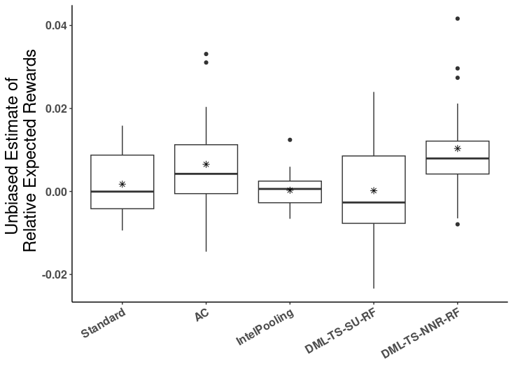
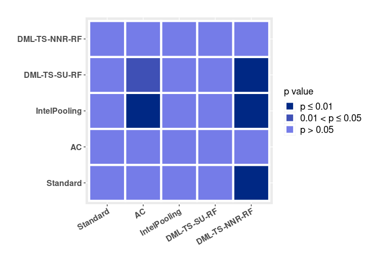
Figure 7: (left) Unbiased estimates of the average per-trial reward for all five competing algorithms, relative to the reward obtained under the pre-specified Valentine randomization policy across 20 multiple-imputed data sets. And (right) p-values from the pairwise paired t-tests. The dark shade in the last column indicates that the proposed DML-TS-NNR-RF algorithm achieved significantly higher rewards than the other three competing algorithms while demonstrating comparable performance to the AC algorithm.

Appendix G Regret Bound

G.1 Double Robustness of Pseudo-Reward

Lemma 2.

If either $p_{i,t}=\pi_{i,t}$ or $f_{i,t}=r_{i,t}$, then

$$\mathbb{E}\left[\tilde{R}_{i,t}^{f}|s,\bar{a}\right] =\Delta_{i,t}(s,\bar{a}).$$

That is, the pseudo-reward is an unbiased estimator of the true differential reward.

Proof.

Recall that

$$\tilde{R}_{i,t}^{f} =\frac{R_{it}-f_{i,t}(s,A_{i,t})}{\delta_{A_{i,t}=\bar{a}}-\pi_{i,t}(0|s)}+\Delta^{f}_{i,t}(s,\bar{a})$$

Case I: $\pi$’s are correctly specified

Then

$$\mathbb{E}\left[\frac{R_{it}}{\delta_{A_{i,t}=\bar{a}}-\pi_{i,t}(0|s)}\biggr{|}s,\bar{a}\right] =r_{i,t}(s,\bar{a})-r_{i,t}(s,0)$$

$$=\Delta_{i,t}(s,\bar{a})$$

and

$$\mathbb{E}\left[\frac{f_{i,t}(s,A_{i,t})}{\delta_{A_{i,t}=\bar{a}}-\pi_{i,t}(0|s)}\biggr{|}s,\bar{a}\right] =f_{i,t}(s,\bar{a})-f_{i,t}(s,0)$$

$$=\Delta^{f}_{i,t}(s,\bar{a})$$

so that

$$\mathbb{E}\left[\frac{R_{it}-f_{i,t}(s,A_{i,t})}{\delta_{A_{i,t}=\bar{a}}-\pi_{i,t}(0|s)}+\Delta^{f}_{i,t}(s,\bar{a})\biggr{|}s,\bar{a}\right] =\Delta_{i,t}(s,\bar{a})-\Delta^{f}_{i,t}(s,\bar{a})+\Delta_{i,t}^{f}(s,\bar{a})$$

$$=\Delta_{i,t}(s,\bar{a})$$

Case II: $f$ correctly specified

$$\mathbb{E}\left[\frac{R_{it}}{\delta_{A_{i,t}=\bar{a}}-\pi_{i,t}(0|s)}\biggr{|}s,\bar{a}\right] =\frac{1-p_{i,t}(0|s)}{1-\pi_{i,t}(0|s)}r_{i,t}(s,\bar{a})-\frac{p_{i,t}(0|s)}{\pi_{i,t}(0|s)}r_{i,t}(s,0)$$

and

$$\mathbb{E}\left[\frac{f_{i,t}(s,A_{i,t})}{\delta_{A_{i,t}=\bar{a}}-\pi_{i,t}(0|s)}\biggr{|}s,\bar{a}\right] =\frac{1-p_{i,t}(0|s)}{1-\pi_{i,t}(0|s)}f_{i,t}(s,\bar{a})-\frac{p_{i,t}(0|s)}{\pi_{i,t}(0|s)}f_{i,t}(s,\bar{0})$$

$$=\frac{1-p_{i,t}(0|s)}{1-\pi_{i,t}(0|s)}r_{i,t}(s,\bar{a})-\frac{p_{i,t}(0|s)}{\pi_{i,t}(0|s)}r_{i,t}(s,\bar{0})$$

and

$$\mathbb{E}\left[\Delta^{f}_{i,t}(s,\bar{a})\biggr{|}s,\bar{a}\right] =\Delta_{i,t}(s,\bar{a})$$

$$\mathbb{E}\left[\frac{R_{it}-f_{i,t}(s,\bar{A}_{i,t})}{\delta_{A_{i,t}=\bar{a}}-\pi_{i,t}(0|s)}+\Delta^{f}_{i,t}(s,\bar{a})\biggr{|}s,\bar{a}\right] =\Delta_{i,t}(s,\bar{a})$$

∎

G.2 Preliminaries

Lemma 3.

Let $X$ be a mean-zero sub-Gaussian random variable with variance factor $v^{2}$ and $Y$ be a bounded random variable such that $|Y|\leq B$ for some $0\leq B<\infty$. Then $XY$ is sub-Gaussian with variance factor $v^{2}B^{2}$.

Proof.

Recall that $X$ being mean-zero sub-Gaussian means that

$$P(|X|\geq t) \leq 2\exp\left(-\frac{t^{2}}{2v^{2}}\right).$$

Now note that

$$|XY| \leq|X|B$$

so that if $|XY|>t$, then $|X|B>t$. Thus by monotonicity

$$P(|XY|\geq t) \leq P(|X|B\geq t)$$

$$=P\left(|X|\geq\frac{t}{B}\right)$$

$$\leq 2\exp\left(-\frac{t^{2}}{2B^{2}v^{2}}\right)$$

as desired. ∎

Lemma 4.

If $X,Y$ are sub-Gaussian with variance factors $v_{x}^{2}$, $v_{y}^{2}$, respectively, then $\alpha X+\beta Y$ is sub-Gaussian with variance factor $\alpha^{2}v_{x}^{2}+\beta^{2}v_{y}^{2}$$\forall\alpha,\beta\in\mathbb{R}$.

Proof.

Recall the equivalent definition of sub-Gaussianity that $X,Y$ are sub-Gaussian iff for some $b,a>0$ and all $\lambda>0$

$$\mathbb{E}\exp\left(\lambda(X-\mathbb{E}X)\right) \leq\exp(\lambda^{2}v_{x}^{2}/2)$$

$$\mathbb{E}\exp\left(\lambda(Y-\mathbb{E}Y)\right) \leq\exp(\lambda^{2}v_{y}^{2}/2)$$

Then

$$\mathbb{E}\exp\left(\lambda(\alpha X+\beta Y-\alpha\mathbb{E}X-\beta\mathbb{E}Y)\right) \leq\sqrt{\mathbb{E}\exp\left(2\alpha\lambda(X-\mathbb{E}X)\right)}\sqrt{\mathbb{E}\exp\left(2\beta\lambda(Y-\mathbb{E}Y)\right)}$$

$$\leq\sqrt{\exp(2\alpha^{2}\lambda^{2}v_{x}^{2})}\sqrt{\exp(2\beta^{2}\lambda^{2}v_{y}^{2})}$$

$$=\exp((\alpha^{2}v_{x}^{2}+\beta^{2}v_{y}^{2})\lambda^{2})$$

∎

The following Lemma gives the sub-Gaussianity and variance of the difference between the pseudo-reward and its expectation. We see that in the variance, all terms except those involving the inverse propensity weighted noise variance vanish as $f_{i,t}$ becomes a better estimate of $r_{i,t}$. Note that means and variances may be implicitly conditioned on the history.

Lemma 5.

If $\pi_{i,t}$ is correctly specified and $\tilde{\sigma}_{i,t}^{2}\geq\frac{1}{c}$, the difference between the pseudo-reward and its expectation (taken wrt the action and noise) is mean zero sub-Gaussian with variance

$$\textrm{Var}\left(\tilde{R}_{i,t}^{f}(s,\bar{a})\right) =\frac{(r_{i,t}(s,\bar{a})-f_{i,t}(s,\bar{a}))^{2}\pi_{i,t}(0|s)+\textrm{Var}(\epsilon_{i,t})}{1-\pi_{i,t}(0|s)}$$

$$\qquad+\frac{(r_{i,t}(s,0)-f_{i,t}(s,0))^{2}[1-\pi_{i,t}(0|s)]+\textrm{Var}(\epsilon_{i,t})}{\pi_{i,t}(0|s)}$$

$$\qquad+2(r_{i,t}(s,\bar{a})-f_{i,t}(s,\bar{a}))(r_{i,t}(s,0)-f_{i,t}(s,0))$$

Proof.

We need to show that it is sub-Gaussian and upper bound its variance. We write the difference as

$$\tilde{R}_{i,t}^{f}(s,\bar{a})-\mathbb{E}[\tilde{R}_{i,t}^{f}|s,\bar{a}] =\tilde{R}_{i,t}^{f}(s,\bar{a})-\Delta_{i,t}(s,\bar{a})$$

$$=\frac{R_{it}-f_{i,t}(s,A_{i,t})}{\delta_{A_{i,t}=\bar{a}}-\pi_{i,t}(0|s)}+\Delta^{f}_{i,t}(s,\bar{a})-\Delta_{i,t}(s,\bar{a})$$

$$=\frac{r_{i,t}(s,A_{i,t})-f_{i,t}(s,A_{i,t})+\epsilon_{i,t}}{\delta_{A_{i,t}=\bar{a}}-\pi_{i,t}(0|s)}+\Delta^{f}_{i,t}(s,\bar{a})-\Delta_{i,t}(s,\bar{a})$$

Note that $|r_{i,t}(s,A_{i,t})|\leq\max\left(|r_{i,t}(s,\bar{a})|,|r_{i,t}(s,0)|\right)$ and $|f_{i,t}(s,A_{i,t})|\leq\max\left(|f_{i,t}(s,\bar{a})|,|f_{i,t}(s,0)|\right)$. Thus since $\left|\frac{1}{\delta_{A_{i,t}=\bar{a}}-\pi_{i,t}(0|s)}\right|$ is upper bounded by $c>0$, we have that $\frac{r_{i,t}(s,A_{i,t})-f_{i,t}(s,A_{i,t})}{\delta_{A_{i,t}=\bar{a}}-\pi_{i,t}(0|s)}$ is bounded and thus (not necessarily mean zero) sub-Gaussian. Since $\epsilon_{i,t}$ is sub-Gaussian, its denominator is bounded, and the remaining terms are deterministic, the entire difference between the pseudo-reward and its mean is sub-Gaussian. Now

$$\textrm{Var}(\tilde{R}_{i,t}^{f}(s,\bar{a})-\mathbb{E}[\tilde{R}_{i,t}^{f}|s,\bar{a}]) =\textrm{Var}\left(\tilde{R}_{i,t}^{f}(s,\bar{a})\right)$$

$$=\mathbb{E}\left[\tilde{R}_{i,t}^{f}(s,\bar{a})^{2}\right]-\Delta_{i,t}(s,\bar{a})^{2}$$ (8)

since $\mathbb{E}[\tilde{R}_{i,t}^{f}|s,\bar{a}]$ is not random. Now we expand the first term on the rhs.

$$\mathbb{E}\left[\tilde{R}_{i,t}^{f}(s,\bar{a})^{2}\right] =\mathbb{E}\left[\left(\frac{r_{i,t}(s,A_{i,t})-f_{i,t}(s,A_{i,t})+\epsilon_{i,t}}{\delta_{A_{i,t}=\bar{a}}-\pi_{i,t}(0|s)}+\Delta_{i,t}^{f}(s,\bar{a})\right)^{2}\right]$$

$$=\mathbb{E}\left[\left(\frac{r_{i,t}(s,A_{i,t})-f_{i,t}(s,A_{i,t})+\epsilon_{i,t}}{\delta_{A_{i,t}=\bar{a}}-\pi_{i,t}(0|s)}\right)^{2}\right]$$

$$\qquad+2\mathbb{E}\left[\frac{r_{i,t}(s,A_{i,t})-f_{i,t}(s,A_{i,t})+\epsilon_{i,t}}{\delta_{A_{i,t}=\bar{a}}-\pi_{i,t}(0|s)}\right]\Delta_{i,t}^{f}(s,\bar{a})+\Delta_{i,t}^{f}(s,\bar{a})^{2}$$

$$=\mathbb{E}\left[\left(\frac{r_{i,t}(s,A_{i,t})-f_{i,t}(s,A_{i,t})+\epsilon_{i,t}}{\delta_{A_{i,t}=\bar{a}}-\pi_{i,t}(0|s)}\right)^{2}\right]$$

$$\qquad+2(\Delta_{i,t}(s,\bar{a})-\Delta_{i,t}^{f}(s,\bar{a}))\Delta_{i,t}^{f}(s,\bar{a})+\Delta_{i,t}^{f}(s,\bar{a})^{2}$$ (9)

For the first term on the rhs of Eqn. 9,

$$\mathbb{E} \left[\left(\frac{r_{i,t}(s,A_{i,t})-f_{i,t}(s,A_{i,t})+\epsilon_{i,t}}{\delta_{A_{i,t}=\bar{a}}-\pi_{i,t}(0|s)}\right)^{2}\right]$$

$$=\mathbb{E}\left[\left(\frac{r_{i,t}(s,A_{i,t})-f_{i,t}(s,A_{i,t})}{\delta_{A_{i,t}=\bar{a}}-\pi_{i,t}(0|s)}\right)^{2}\right]+\mathbb{E}\left[\left(\frac{\epsilon_{i,t}}{\delta_{A_{i,t}=\bar{a}}-\pi_{i,t}(0|s)}\right)^{2}\right]$$

$$=\frac{(r_{i,t}(s,\bar{a})-f_{i,t}(s,\bar{a}))^{2}+\mathbb{E}[\epsilon_{i,t}^{2}]}{1-\pi_{i,t}(0|s)}+\frac{(r_{i,t}(s,0)-f_{i,t}(s,0))^{2}+\mathbb{E}[\epsilon_{i,t}^{2}]}{\pi_{i,t}(0|s)}$$

so that plugging this into Eqn. 9, we have

$$\mathbb{E}\left[\tilde{R}_{i,t}^{f}(s,\bar{a})^{2}\right] =\frac{(r_{i,t}(s,\bar{a})-f_{i,t}(s,\bar{a}))^{2}+\mathbb{E}[\epsilon_{i,t}^{2}]}{1-\pi_{i,t}(0|s)}+\frac{(r_{i,t}(s,0)-f_{i,t}(s,0))^{2}+\mathbb{E}[\epsilon_{i,t}^{2}]}{\pi_{i,t}(0|s)}$$

$$\qquad+2(\Delta_{i,t}(s,\bar{a})-\Delta_{i,t}^{f}(s,\bar{a}))\Delta_{i,t}^{f}(s,\bar{a})+\Delta_{i,t}^{f}(s,\bar{a})^{2}$$

and plugging this into Eqn. 8 we obtain the variance.

$$\textrm{Var}\left(\tilde{R}_{i,t}^{f}(s,\bar{a})\right) =\frac{(r_{i,t}(s,\bar{a})-f_{i,t}(s,\bar{a}))^{2}+\textrm{Var}(\epsilon_{i,t})}{1-\pi_{i,t}(0|s)}+\frac{(r_{i,t}(s,0)-f_{i,t}(s,0))^{2}+\textrm{Var}(\epsilon_{i,t})}{\pi_{i,t}(0|s)}$$

$$\qquad+2(\Delta_{i,t}(s,\bar{a})-\Delta_{i,t}^{f}(s,\bar{a}))\Delta_{i,t}^{f}(s,\bar{a})+\Delta_{i,t}^{f}(s,\bar{a})^{2}-\Delta_{i,t}(s,\bar{a})^{2}$$ (10)

Note that

$$2(\Delta_{i,t}(s,\bar{a})-\Delta_{i,t}^{f}(s,\bar{a}))\Delta_{i,t}^{f}(s,\bar{a})+\Delta_{i,t}^{f}(s,\bar{a})^{2}-\Delta_{i,t}(s,\bar{a})^{2}$$

$$=2(\Delta_{i,t}(s,\bar{a})-\Delta_{i,t}^{f}(s,\bar{a}))\Delta_{i,t}^{f}(s,\bar{a})-(\Delta_{i,t}(s,\bar{a})-\Delta_{i,t}^{f}(s,\bar{a}))(\Delta_{i,t}(s,\bar{a})+\Delta_{i,t}^{f}(s,\bar{a}))$$

$$=(\Delta_{i,t}(s,\bar{a})-\Delta_{i,t}^{f}(s,\bar{a}))(\Delta_{i,t}^{f}(s,\bar{a})-\Delta_{i,t}(s,\bar{a}))$$

$$=-(\Delta_{i,t}(s,\bar{a})-\Delta_{i,t}^{f}(s,\bar{a}))^{2}$$

and plugging this into Eqn. 10,

$$\textrm{Var}\left(\tilde{R}_{i,t}^{f}(s,\bar{a})\right) =\frac{(r_{i,t}(s,\bar{a})-f_{i,t}(s,\bar{a}))^{2}+\textrm{Var}(\epsilon_{i,t})}{1-\pi_{i,t}(0|s)}+\frac{(r_{i,t}(s,0)-f_{i,t}(s,0))^{2}+\textrm{Var}(\epsilon_{i,t})}{\pi_{i,t}(0|s)}$$

$$\qquad-(\Delta_{i,t}(s,\bar{a})-\Delta_{i,t}^{f}(s,\bar{a}))^{2}$$

as desired. Now note that

$$\left(\Delta_{i,t}(s,\bar{a})-\Delta_{i,t}^{f}(s,\bar{a})\right)^{2} =\left(r_{i,t}(s,\bar{a})-r_{i,t}(s,0)-(f_{i,t}(s,\bar{a})-f_{i,t}(s,0))\right)^{2}$$

$$=\left(r_{i,t}(s,\bar{a})-f_{i,t}(s,\bar{a})-(r_{i,t}(s,0)-f_{i,t}(s,0))\right)^{2}$$

$$=(r_{i,t}(s,\bar{a})-f_{i,t}(s,\bar{a}))^{2}+(r_{i,t}(s,0)-f_{i,t}(s,0))^{2}$$

$$\qquad+2(r_{i,t}(s,\bar{a})-f_{i,t}(s,\bar{a}))(r_{i,t}(s,0)-f_{i,t}(s,0))$$

so that

$$\textrm{Var}\left(\tilde{R}_{i,t}^{f}(s,\bar{a})\right) =\frac{(r_{i,t}(s,\bar{a})-f_{i,t}(s,\bar{a}))^{2}\pi_{i,t}(0|s)+\textrm{Var}(\epsilon_{i,t})}{1-\pi_{i,t}(0|s)}$$

$$\qquad+\frac{(r_{i,t}(s,0)-f_{i,t}(s,0))^{2}[1-\pi_{i,t}(0|s)]+\textrm{Var}(\epsilon_{i,t})}{\pi_{i,t}(0|s)}$$

$$\qquad+2(r_{i,t}(s,\bar{a})-f_{i,t}(s,\bar{a}))(r_{i,t}(s,0)-f_{i,t}(s,0))$$

∎

Corollary 1.

$$\mathbb{E}_{p(s,\bar{a})}\left[\textrm{Var}\left(\tilde{R}_{i,t}^{f}(s,\bar{a})\right)\right] \leq\frac{\mathbb{E}_{p(s,\bar{a})}\left[(r_{i,t}(s,\bar{a})-f_{i,t}(s,\bar{a}))^{2}\right]\pi_{i,t}(0|s)+\textrm{Var}(\epsilon_{i,t})}{1-\pi_{i,t}(0|s)}$$

$$\qquad+\frac{\mathbb{E}_{p(s,\bar{a})}\left[(r_{i,t}(s,0)-f_{i,t}(s,0))^{2}\right][1-\pi_{i,t}(0|s)]+\textrm{Var}(\epsilon_{i,t})}{\pi_{i,t}(0|s)}$$

$$\qquad+2\sqrt{\mathbb{E}_{p(s,\bar{a})}\left[(r_{i,t}(s,\bar{a})-f_{i,t}(s,\bar{a}))^{2}\right]}\sqrt{\mathbb{E}_{p(s)}\left[(r_{i,t}(s,0)-f_{i,t}(s,0))^{2}\right]}$$

Proof.

It follows immediately by taking expectations and applying Cauchy Schwartz. ∎

Corollary 2.

$(r_{i,t}(\cdot,0)-f_{i,t}(\cdot,0))^{2}=o_{P}(k^{-1/2})$ and $(r_{i,t}(\cdot,\bar{a})-f_{i,t}(\cdot,\bar{a}))^{2}=o_{P}(k^{-1/2})$

Proof.

Note that

$$P\left((r_{i,t}(\cdot,0)-f_{i,t}(\cdot,0))^{2}k^{1/2}>C\right) \leq\frac{\mathbb{E}_{p(\mathcal{H}_{k-1})}\mathbb{E}_{p(s)}\left[(r_{i,t}(s,0)-f_{i,t}(s,0))^{2}\right]k^{1/2}}{C}$$

$$=\frac{\mathbb{E}_{p(\mathcal{H}_{k-1})}o_{P}(k^{-1/2})k^{1/2}}{C}\textrm{ Assumption \ref{assm:ml-model-convergence-rate}}$$

$$=\frac{\mathbb{E}_{p(\mathcal{H}_{k-1})}o_{P}(1)}{C}$$

$$\leq\delta\textrm{ for sufficiently large $k$}$$

so that $(r_{i,t}(\cdot,0)-f_{i,t}(\cdot,0))^{2}=o_{P}(k^{-1/2})$. In the second to last line we used that since $r_{i,t},f_{i,t}$ are bounded, $\mathbb{E}_{p(s)}\left[(r_{i,t}(s,0)-f_{i,t}(s,0))^{2}\right]$ is bounded. For bounded random variables, convergence in probability implies convergence in mean. A similar result holds when using $\bar{a}$ instead of $0$. ∎

Corollary 3.

$$\textrm{Var}\left(\tilde{R}_{i,t}^{f}(s,\bar{a})\right) \leq\frac{o_{P}(k^{-1/2})\pi_{i,t}(0|s)+\textrm{Var}(\epsilon_{i,t})}{1-\pi_{i,t}(0|s)}+\frac{o_{P}(k^{-1/2})[1-\pi_{i,t}(0|s)]+\textrm{Var}(\epsilon_{i,t})+\textrm{Var}(\epsilon_{i,t})}{\pi_{i,t}(0|s)}$$

$$\qquad+2o_{P}(k^{-1/2})$$

Proof.

This follows immediately from the previous two Corollaries. ∎

Corollary 4.

For all $\delta>0$, there exists $C>0$ s.t. w.p. at least $1-\delta$,

$$\textrm{Var}\left(\tilde{R}_{i,t}^{f}(s,\bar{a})\right) \leq\frac{Ck^{-1/2}\pi_{i,t}(0|s)+\textrm{Var}(\epsilon_{i,t})}{1-\pi_{i,t}(0|s)}+\frac{Ck^{-1/2}[1-\pi_{i,t}(0|s)]+\textrm{Var}(\epsilon_{i,t})}{\pi_{i,t}(0|s)}+2Ck^{-1/2}.$$

We define denote the rhs as $v_{k}^{2}$ e.g.

$$v_{k}^{2} \equiv\frac{Ck^{-1/2}\pi_{i,t}(0|s)+\textrm{Var}(\epsilon_{i,t})}{1-\pi_{i,t}(0|s)}+\frac{Ck^{-1/2}[1-\pi_{i,t}(0|s)]+\textrm{Var}(\epsilon_{i,t})}{\pi_{i,t}(0|s)}+2Ck^{-1/2}$$

Proof.

By the definition of $o_{P}$, if $(f_{i,t}-r_{i,t})^{2}=o_{P}(k^{-1/2})$ for any $A>0,\delta>0$, there exists $K$ s.t. if $K>k$, then w.p. at least $1-\delta$,

$$(f_{i,t}-r_{i,t})^{2}\leq Ak^{-1/2}.$$

Then for all $k\in\mathbb{N}$, since $f,r$ are bounded

$$(f_{i,t}-r_{i,t})^{2} \leq 16B^{2}I(k\leq K)+I(k>K)Ak^{-1/2}.$$

Now choose

$$C \equiv\max\left(A,16B^{2}\right).$$

∎

In the next remark, we show what the variance would be if we did not use DML and estimate $f_{i,t}\approx r_{i,t}$, but used only the inverse propensity weighted observed reward as the pseudo-reward. This was done in Greenewald et al. (2017). In this case, there are terms dependent on the mean reward that do not vanish as the number of stages goes to infinity.

Remark 2.

If we instead used as our pseudo-reward the inverse propensity weighted observed reward

$$\tilde{R}_{i,t}(s,\bar{a}) =\frac{R_{it}}{\delta_{A_{i,t}=\bar{a}}-\pi_{i,t}(0|s)}$$

this would be unbiased with variance

$$v_{k}^{2}\equiv\frac{r_{i,t}(s,\bar{a})^{2}+\textrm{Var}(\epsilon_{i,t})}{1-\pi_{i,t}(0|s)}+\frac{r_{i,t}(s,0)^{2}+\textrm{Var}(\epsilon_{i,t})}{\pi_{i,t}(0|s)}-\Delta_{i,t}(s,\bar{a})^{2}$$

Proof.

The unbiasedness is clear from our proof of Lemma 2. For the variance,

$$\textrm{Var}\left(\frac{R_{it}}{\delta_{A_{i,t}=\bar{a}}-\pi_{i,t}(0|s)}\right) =\mathbb{E}\left[\frac{(r_{i,t}(s,\bar{a})+\epsilon_{i,t})^{2}}{1-\pi_{i,t}(0|s)}+\frac{(r_{i,t}(s,0)+\epsilon_{i,t})^{2}}{\pi_{i,t}(0|s)}\right]-\Delta_{i,t}(s,\bar{a})^{2}$$

$$=\frac{r_{i,t}(s,\bar{a})^{2}+\textrm{Var}(\epsilon_{i,t})}{1-\pi_{i,t}(0|s)}+\frac{r_{i,t}(s,0)^{2}+\textrm{Var}(\epsilon_{i,t})}{\pi_{i,t}(0|s)}-\Delta_{i,t}(s,\bar{a})^{2}$$

$$=\frac{r_{i,t}(s,\bar{a})^{2}+\textrm{Var}(\epsilon_{i,t})}{1-\pi_{i,t}(0|s)}+\frac{r_{i,t}(s,0)^{2}+\textrm{Var}(\epsilon_{i,t})}{\pi_{i,t}(0|s)}$$

$$\qquad-(r_{i,t}(s,\bar{a})-r_{i,t}(s,0))^{2}$$

$$=\frac{r_{i,t}(s,\bar{a})^{2}+\textrm{Var}(\epsilon_{i,t})}{1-\pi_{i,t}(0|s)}-r_{i,t}(s,\bar{a})^{2}+\frac{r_{i,t}(s,0)^{2}+\textrm{Var}(\epsilon_{i,t})}{\pi_{i,t}(0|s)}$$

$$\qquad-r_{i,t}(s,0)^{2}+2r_{i,t}(s,\bar{a})r_{i,t}(s,0)$$

$$=\frac{r_{i,t}(s,\bar{a})^{2}\pi_{i,t}(0,s)+\textrm{Var}(\epsilon_{i,t})}{1-\pi_{i,t}(0|s)}+\frac{r_{i,t}(s,0)^{2}[1-\pi_{i,t}(0|s)]+\textrm{Var}(\epsilon_{i,t})}{\pi_{i,t}(0|s)}$$

$$\qquad+2r_{i,t}(s,\bar{a})r_{i,t}(s,0)$$

∎

Here we collect three important results. For analysis at stage $K$, let $\phi(x_{i,t})$ encodes the vector $x_{i,t}$ for the $i$th individual and the $t$th time in a vector of length $2d*K$. At stage $k$, let $\mathcal{O}_{k}$ denote the set of observed time points across all individuals at stage $k$. Let $\hat{\theta}_{k}$ denote the estimates for stage $k+1$ using data from $\mathcal{O}_{k}$. First, we prove a slightly modified version of Lemma 10 from Abbasi-Yadkori et al. (2011):

Lemma 6.

(Determinant-Trace Inequality) Suppose $\tilde{\sigma}_{i,t}\phi(\boldsymbol{x}_{i,t})\in\mathbb{R}^{d}$. Let $V_{k+1}=\sum_{(i,t)\in\mathcal{O}_{k}}\tilde{\sigma}_{i,t}^{2}\phi(\boldsymbol{x}_{i,t})\phi(\boldsymbol{x}_{i,t})^{\top}+V_{0}$. Then

$$\det(V_{k+1}) \leq\left(\frac{4\textrm{tr}(V_{0})+|\mathcal{O}_{k}|}{4d}\right)^{d}$$

Proof.

Following the arguments for the proof of the original Lemma 11 in Abbasi-Yadkori et al. (2011), we have

$$\textrm{det}(V_{k+1}) \leq\left(\frac{\textrm{tr}(V_{k+1})}{d}\right)^{d}.$$

Now we have $\textrm{tr}(\tilde{\sigma}_{i,t}^{2}\phi(\boldsymbol{x}_{i,t})\phi(\boldsymbol{x}_{i,t})^{\top})\leq 1/4$ since $\|x_{i,t}\|\leq 1$ and $\tilde{\sigma}_{i,t}^{2}\leq(1/2)^{2}$.

$$\textrm{tr}(V_{k+1}) =\textrm{tr}(V_{0})+\sum_{(i,t)\in\mathcal{O}_{k}}\tilde{\sigma}_{i,t}^{2}\textrm{tr}(\phi(\boldsymbol{x}_{i,t})\phi(\boldsymbol{x}_{i,t})^{\top})$$

$$=\textrm{tr}(V_{0})+\sum_{(i,t)\in\mathcal{O}_{k}}\tilde{\sigma}_{i,t}^{2}\|\phi(\boldsymbol{x}_{i,t})\|^{2}_{2}$$

$$\leq\textrm{tr}(V_{0})+\frac{1}{4}|\mathcal{O}_{k}|$$

Plugging this in to the rhs of the determinant inequality in the first step gives the desired result. ∎

We adapt an important concentration inequality for regularized least-squares estimates. Our proof follows the same basic strategy as Abbasi-Yadkori et al. (2011), but with modifications due to 1) the use of weighted least squares 2) the use of pseudo-rewards to estimate differential rewards 3) replacing the scaled diagonal regularization with Laplacian regularization.

Lemma 7 (Adapted from Theorem 2 in Abbasi-Yadkori et al. (2011)).

For any $\delta>0$, w.p. at least $1-\delta$ the estimates $\{\hat{\Theta}_{k}\}_{k=0}^{\infty}$ in Algorithm 1 satisfies for any $\{x_{k}\}_{k=0}^{\infty}$,

$$|x_{k}^{\top}(\hat{\Theta}_{k}-\Theta^{*}_{k})| \leq\|x_{k}\|_{V_{k-1}^{-1}}\left(v_{k}\sqrt{2\log\left(\frac{\det(V_{k-1})^{1/2}\det(V_{0})^{-1/2}}{\delta}\right)}+\lambda_{\max}(V_{0})^{1/2}kB\right),$$ (11)

where $v_{k}^{2}$ is the variance factor for the difference between the pseudo-reward and its mean at stage $k$. In particular, setting $x_{k}=V_{k-1}(\hat{\Theta}_{k-1}-\Theta_{k}^{*})$ implies

$$\|\hat{\Theta}_{k}-\Theta_{k}^{*}\| \leq v_{k}\sqrt{2\log\left(\frac{\det(V_{k-1})^{1/2}\det(V_{0})^{-1/2}}{\delta}\right)}+\lambda_{\max}(V_{0})^{1/2}kB$$

holds w.p. at least $1-\delta$ for all $k\geq 1$.

Proof.

Let $m_{i,t}=\tilde{\sigma}_{i,t}\phi(\textbf{x}_{i,t})$ and $\rho_{i,t}=\tilde{\sigma}_{i,t}[\tilde{R}_{i,t}^{f}(s,\bar{a})-\mathbb{E}[\tilde{R}_{i,t}^{f}|s,\bar{a}]]$. Further let

$$\xi_{k} \equiv\sum_{(i,t)\in\mathcal{O}_{k}}\tilde{\sigma}_{i,t}^{2}[\tilde{R}_{i,t}^{f}(s,\bar{a})-\mathbb{E}[\tilde{R}_{i,t}^{f}|s,\bar{a}]]\phi(\textbf{x}_{i,t})$$

$$=\sum_{(i,t)\in\mathcal{O}_{k}}\tilde{\sigma}_{i,t}[\tilde{R}_{i,t}^{f}(s,\bar{a})-\mathbb{E}[\tilde{R}_{i,t}^{f}|s,\bar{a}]]m_{i,t}$$

$$=\sum_{(i,t)\in\mathcal{O}_{k}}m_{i,t}\rho_{i,t}$$

Then noting that $V_{k}=\sum_{(i,t)\in\mathcal{O}_{k}}m_{i,t}m_{i,t}^{\top}+V_{0}$ and letting $W_{k}$ be the diagonal matrix of weights $\tilde{\sigma}_{i,t}^{2}$, we have

$$\hat{\Theta}_{k} =V_{k-1}^{-1}b_{k}$$

$$=V_{k-1}^{-1}(\xi_{k}+\Phi_{k}^{\top}W_{k}\mathbb{E}[R_{k}^{\hat{f}_{k}}|\bar{a},s])$$

$$=V_{k-1}^{-1}\xi_{k}+V_{k}^{-1}\Phi_{k}^{\top}W_{k}\Delta_{k}\textrm{ by Lemma \ref{lemma:doubly-robust}}$$

$$=V_{k-1}^{-1}\xi_{k}+V_{k-1}^{-1}\Phi_{k}^{\top}W_{k}\Phi_{k}\Theta_{k}^{*}$$

$$=V_{k-1}^{-1}\xi_{k}+V_{k-1}^{-1}(\Phi_{k}^{\top}W_{k}\Phi_{k}+V_{0})\Theta_{k}^{*}-V_{k-1}^{-1}V_{0}\Theta_{k}^{*}$$

$$=V_{k-1}^{-1}\xi_{k}+\Theta_{k}^{*}-V_{k-1}^{-1}V_{0}\Theta_{k}^{*}$$

and thus

$$\hat{\Theta}_{k}-\Theta^{*}_{k} =V_{k-1}^{-1}(\xi_{k}-V_{0}\Theta_{k}^{*})$$

which gives

$$|x_{k}^{\top}\hat{\Theta}_{k}-x_{k}^{\top}\Theta_{k}^{*}| \leq\|x_{k}\|_{V_{k-1}^{-1}}(\|\xi_{k}\|_{V_{k-1}^{-1}}+\|V_{0}\Theta_{k}^{*}\|_{V_{k-1}^{-1}})$$

Now since $\xi_{k}$ is sub-Gaussian with variance factor $v_{k}^{2}$, by Theorem 1 in Abbasi-Yadkori et al. (2011), w.p. $1-\delta$,

$$\|\xi_{k}\|_{V_{k-1}^{-1}}^{2} \leq 2v_{k}^{2}\log\left(\frac{\textrm{det}(V_{k-1})^{1/2}\textrm{det}(V_{0})^{-1/2}}{\delta}\right)$$

Further note

$$\|V_{0}\Theta_{k}^{*}\|_{V_{k-1}^{-1}}^{2} =\Theta_{k}^{*\top}V_{0}^{\top}V_{k-1}^{-1}V_{0}\Theta_{k}^{*}$$

$$\leq\|V_{0}^{\top}V_{k-1}^{-1}V_{0}\|_{2}\|\Theta_{k}^{*}\|_{2}^{2}$$

$$\leq\|V_{0}\|^{2}_{2}\|V_{k-1}^{-1}\|_{2}\|\Theta_{k}^{*}\|_{2}^{2}$$

$$\leq\lambda_{\textrm{max}}(V_{0})\|\Theta_{k}^{*}\|_{2}^{2}$$

$$\leq\lambda_{\textrm{max}}(V_{0})k^{2}B^{2}$$

and thus

$$|x_{k}^{\top}\hat{\Theta}_{k}-x_{k}^{\top}\Theta_{k}^{*}| \leq\|x_{k}\|_{V_{k-1}^{-1}}\left(v_{k}\sqrt{2\log\left(\frac{\textrm{det}(V_{k-1}^{-1})^{1/2}\textrm{det}(V_{0})^{-1/2}}{\delta}\right)}+\lambda_{\max}(V_{0})^{1/2}kB\right)$$

Corollary 5.

If Assumption 3, then for any $\delta>0$, there exists $C>0$ s.t. w.p. at least $1-\delta$ the estimates $\{\hat{\Theta}_{k}\}_{k=0}^{\infty}$ in Algorithm 1 satisfies for any $\{x_{k}\}_{k=0}^{\infty}$,

$$|x_{k}^{\top}(\hat{\Theta}_{k}-\Theta^{*}_{k})| \leq\|x_{k}\|_{V_{k-1}^{-1}}\left(\left(\frac{C}{k^{1/2}}+\sigma^{2}c^{2}\right)\sqrt{2\log\left(\frac{\det(V_{k-1})^{1/2}\det(V_{0})^{-1/2}}{\delta/2}\right)}+\lambda_{\max}(V_{0})^{1/2}kB\right),$$ (12)

In particular, setting $x_{k}=V_{k-1}(\hat{\Theta}_{k-1}-\Theta_{k}^{*})$ implies

$$\|\hat{\Theta}_{k}-\Theta_{k}^{*}\| \leq\left(\frac{C}{k^{1/2}}+\sigma^{2}c^{2}\right)\sqrt{2\log\left(\frac{\det(V_{k-1})^{1/2}\det(V_{0})^{-1/2}}{\delta/2}\right)}+\lambda_{\max}(V_{0})^{1/2}kB$$

holds w.p. at least $1-\delta$ for all $k\geq 1$.

Proof.

Use Corollary 3 and Lemma 7, each with $\delta/2$. Then w.p. at least $1-\delta$ the result holds. ∎

∎

We next state a slightly modified form of a standard result of RLS (Lemma 11 in Abbasi-Yadkori et al. (2011)) that helps to guarantee that the prediction error is cumulatively small. This bounds the sum of quadratic forms where the matrix is the inverse Gram matrix and the arguments are the feature vectors. We use such terms to construct a martingale in the regret bound so that we can bound such terms and the martingale.

Proposition 1.

Let $\lambda\geq 1$ and $\gamma\geq 1$. For any arbitrary sequence $(\boldsymbol{x}_{i,t})_{(i,t)\in\mathcal{O}_{k}}$, let

$$V_{k+1}\equiv\sum_{(i,t)\in\mathcal{O}_{k}}\tilde{\sigma}_{i,t}^{2}\phi(\boldsymbol{x}_{i,t})\phi(\boldsymbol{x}_{i,t})^{\top}+V_{0},$$

be the regularized Gram matrix. Then

$$\sum_{k=1}^{K}\sum_{(i,t)\in\mathcal{O}_{k}\backslash\mathcal{O}_{k-1}}\|\phi(\boldsymbol{x}_{i,t})\|_{V_{k}^{-1}}^{2}\leq 2c\log\left(\frac{\det(V_{K+1})}{\det(V_{0})}\right).$$

where $c$ is a constant such that $0<\frac{1}{c}<\tilde{\sigma}_{i,t}^{2}\forall i,t\in\mathbb{N}$. Further,

$$\log\det(V_{K+1}) \leq 2Kd\log\left(\left[\gamma+\lambda M+\frac{K+1}{8d}\right]\right)$$

Proof.

By Lemma $11$ in Abbasi-Yadkori et al. (2011), we have

$$\sum_{k=1}^{K}\sum_{(i,t)\in\mathcal{O}_{k}\backslash\mathcal{O}_{k-1}}\tilde{\sigma}_{i,t}^{2}\|\phi(\boldsymbol{x}_{i,t})\|_{V_{k}^{-1}}^{2}\leq 2\log\left(\frac{\det(V_{K+1})}{\det(V_{0})}\right).$$

The lower bound on the weights implies

$$\sum_{k=1}^{K}\sum_{(i,t)\in\mathcal{O}_{k}\backslash\mathcal{O}_{k-1}}\|\phi(\boldsymbol{x}_{i,t})\|_{V_{k}^{-1}}^{2} \leq 2c\log\left(\frac{\det(V_{K+1})}{\det(V_{0})}\right)$$

as desired.

By definition, we have $tr(\tilde{\sigma}_{i,t}^{2}\phi(\boldsymbol{x}_{i,t})\phi(\boldsymbol{x}_{i,t})^{\top})\leq 2/4$ since $\|x_{i,t}\|\leq 1$ and $\tilde{\sigma}_{i,t}^{2}\leq(1/2)^{2}$; and $tr(L_{\otimes})=tr(L)\cdot tr(I)=KMd$. Then by Hadamard’s inequality we have

$$\log\det(V_{K+1}) \leq 2Kd\log\left(\frac{1}{2Kd}\text{tr}\left(V_{K+1}\right)\right)$$

$$=2Kd\log\left(\frac{1}{2Kd}\left[\gamma 2Kd+\lambda 2KMd+\frac{2}{4}K\cdot(K+1)/2\right]\right)$$

$$=2Kd\log\left(\left[\gamma+\lambda M+\frac{K+1}{8d}\right]\right)$$

∎

Finally, we state Azuma’s concentration inequality which describes concentration of super-martingales with bounded differences and is useful in controlling the regret due to the randomization of Thompson sampling.

Proposition 2 (Azuma’s concentration inequality).

If a super-martingale $(Y_{t})_{t\geq 0}$ corresponding to a filtration $\mathcal{F}_{t}$ satisfies $|Y_{t}-Y_{t-1}|<c_{t}$ some constant $c_{t}$ for all $t=1,\ldots,T$ then for any $\alpha>0$:

$$P\left(Y_{T}-Y_{0}\geq\alpha\right)\leq\exp\left(-\frac{\alpha^{2}}{2\sum_{t=1}^{T}c_{t}^{2}}\right).$$

G.3 Proof of Theorem 1

The proof follows closely from Abeille & Lazaric (2017) with several adjustments. Assumption 2 implies that we only need to consider the unit ball $\mathcal{X}=\{\|x\|\leq 1\}$. Then the regret can be decomposed into

$$\underbrace{\sum_{k=1}^{K}\frac{1}{k}\sum_{(i,t)\in\mathcal{O}_{k}\backslash\mathcal{O}_{k-1}}\left((\phi(x_{i,t}^{\star}))^{\top}\Theta^{\star}_{k}-\phi(x_{i,t})^{\top}\tilde{\Theta}_{k}\right)}_{R^{TS}(K)}+\underbrace{\sum_{k=1}^{K}\frac{1}{k}\sum_{(i,t)\in\mathcal{O}_{k}\backslash\mathcal{O}_{k-1}}\left(\phi(x_{i,t})^{\top}\tilde{\Theta}_{k}-\phi(x_{i,t})^{\top}\Theta^{\star}_{k}\right)}_{R^{RLS}(K)}$$

where $\phi(x_{i,t}^{\star})$ is the context vector under the optimal action and $\Theta^{\star}_{k}$ is the true parameter value. The first term is the regret due to the random deviations caused by sampling $\tilde{\Theta}_{k}$ and whether it provides sufficient useful information about the true parameter $\Theta^{\star}_{k}$. The second term is the concentration of the sampled term around the true linear model for the advantage function.

Definition 2.

We define the filtration $\mathcal{F}_{k}$ as the information accumulated up to stage $k$ before the sampling procedure, that is, $\mathcal{F}_{k}=(\mathcal{F}_{1},\sigma(x_{1},r_{2},x_{2},\ldots,x_{k-1},r_{k-1}))$, and filtration $\mathcal{F}_{k}^{x}$ as the information accumulated up to stage $k$ and including the sampled context, that is, $\mathcal{F}_{t}=(\mathcal{F}_{1},\sigma(x_{1},r_{2},x_{2},\ldots,x_{k-1},r_{k-1},x_{k}))$.

Bounding $R^{RLS}(T)$.

We decompose the second term into the variation of the point estimate and the variation of the random sample around the point estimate:

$$\sum_{k=1}^{K}\frac{1}{k}\sum_{(i,t)\in\mathcal{O}_{k}\backslash\mathcal{O}_{k-1}}\left(\phi(x_{i,t})^{\top}\tilde{\Theta}_{k}-\phi(x_{i,t})^{\top}\hat{\Theta}_{k}\right)+\sum_{k=1}^{K}\frac{1}{k}\sum_{(i,t)\in\mathcal{O}_{k}\backslash\mathcal{O}_{k-1}}\left(\phi(x_{i,t})^{\top}\hat{\Theta}_{k}-\phi(x_{i,t})^{\top}\Theta^{\star}_{k}\right)$$

The first term describes the deviation of the TS linear predictor from the RLS one, while the second term describes the deviation of the RLS linear predictor from the true linear predictor. The first term is controlled by the construction of the sampling distribution $D^{TS}$, while the second term is controlled by the RLS estimate being a minimizer of the regularized cumulative squared error in (5). In particular, the first term will be small when the TS estimate concentrates around the RLS one, while the second will be small when the RLS estimate concentrates around the true parameter vector. The next proposition gives a lower bound on the probability that, for all stages, both the RLS parameter vector concentrates around the true parameter vector and the TS parameter vector concentrates around the RLS one.

Recall that

$$\beta_{k}(\delta)=v_{k}\left[2\log\left(\frac{\det(V_{k})^{1/2}}{\det(V_{0})^{1/2}\delta/2}\right)\right]^{1/2}+B$$

Proposition 3.

Let $\hat{E}_{k}$ denote the event that $\hat{\Theta}_{k}$ concentrates around the true parameter for all $l\leq k$, i.e., $\hat{E}_{k}=\{\forall l\leq k,\|\hat{\Theta}_{l}-\Theta^{\star}_{l}\|_{V_{l}}\leq\beta_{l}(\delta^{\prime})\}$. Let $\gamma_{k}(\delta)\equiv\beta_{k}(\delta^{\prime})\sqrt{cd\log\frac{c^{\prime}d}{\delta}}$Let $\tilde{E}_{k}$ denote the event that $\tilde{\Theta}_{l}$ concentrates around the estimated parameter for all $l\leq k$, i.e., $\tilde{E}_{k}=\{\forall l\leq k,\|\tilde{\Theta}_{l}-\hat{\Theta}_{l}\|_{V_{l}}\leq\gamma_{l}(\delta^{\prime})\}$. Let $E_{k}=\hat{E}_{k}\cap\tilde{E}_{k}$. Then $P(E_{k})\geq 1-\delta/2$.

Proof.

Let $\delta^{\prime}=\delta/4K$, then Lemma 7 and a union bound give us

$$P(\hat{E}_{K}) =P(\cap_{k=1}^{K}\{\|\Theta_{k}-\Theta^{\star}\|_{V_{k}}\leq\beta_{k}(\delta^{\prime})\})$$

$$=1-\sum_{k=1}^{K}P(\|\Theta_{k}-\Theta^{\star}\|_{V_{k}}>\beta_{k}(\delta^{\prime}))$$

$$=1-\sum_{k=1}^{K}\delta^{\prime}=1-\delta^{\prime}K=1-\delta/4.$$

Applying the TS sampling distribution and $\tilde{\Theta}_{k}=\hat{\Theta}_{k}+\beta_{k}(\delta^{\prime})V_{k}^{-1/2}\eta_{k}$ where $\eta_{t}$ is drawn i.i.d. from $D^{TS}$ we have

$$P\left(\|\tilde{\Theta}_{k}-\hat{\Theta}_{k}\|_{V_{k}}\leq\beta_{k}(\delta^{\prime})\sqrt{cd\log\left(\frac{c^{\prime}d}{\delta^{\prime}}\right)}\right)=P\left(\|\eta_{k}\|\leq\sqrt{cd\log\left(\frac{c^{\prime}d}{\delta^{\prime}}\right)}\right)\geq 1-\delta^{\prime}.$$

by Definition 1. A union-bound argument yields the conclusion. ∎

We can then bound $R^{RLS}(K)$ by leveraging Lemma 7 and decomposing the error via

$$R^{RLS}(K) \leq\sum_{k=1}^{K}\frac{1[E_{K}]}{k}\left[\sum_{(i,t)\in\mathcal{O}_{k}\backslash\mathcal{O}_{k-1}}|\phi(x_{i,t})^{\top}(\tilde{\Theta}_{k}-\hat{\Theta}_{k})|\right]$$

$$+\sum_{k=1}^{K}\frac{1[E_{K}]}{k}\left[\sum_{(i,t)\in\mathcal{O}_{k}\backslash\mathcal{O}_{k-1}}|\phi(x_{i,t})^{\top}(\hat{\Theta}_{k}-\Theta_{k}^{*})|\right]$$

By definition of the event $E_{K}$, we have

$$|\phi(x_{i,t})^{\top}(\tilde{\Theta}_{k}-\hat{\Theta}_{k})|1[E_{k}]\leq\|\phi(x_{i,t})\|_{V_{k}^{-1}}\gamma_{k}(\delta^{\prime}),\quad|\phi(x_{i,t})^{\top}(\hat{\Theta}_{k}-\Theta^{\star})|1[E_{k}]\leq\|\phi(x_{i,t})\|_{V_{k}^{-1}}\beta_{k}(\delta^{\prime})$$

so from Proposition 1, we have

$$\sum_{k=1}^{K}\frac{1[E_{K}]}{k}\left[\sum_{(i,t)\in\mathcal{O}_{k}\backslash\mathcal{O}_{k-1}}|\phi(x_{i,t})^{\top}(\tilde{\Theta}_{k}-\hat{\Theta}_{k})|\right]$$

$$\leq\gamma_{K}(\delta^{\prime})\sum_{k=1}^{K}\left[\sum_{(i,t)\in\mathcal{O}_{k}\backslash\mathcal{O}_{k-1}}\frac{1}{k}\|\phi(x_{i,t})\|_{V_{k}^{-1}}\right]$$

$$\leq\gamma_{K}(\delta^{\prime})\sqrt{\sum_{k=1}^{K}\sum_{(i,t)\in\mathcal{O}_{k}\backslash\mathcal{O}_{k-1}}\frac{1}{k^{2}}}\sqrt{\sum_{k=1}^{K}\sum_{(i,t)\in\mathcal{O}_{k}\backslash\mathcal{O}_{k-1}}\|\phi(x_{i,t})\|_{V_{k}^{-1}}^{2}}$$

$$\leq\gamma_{K}(\delta^{\prime})\sqrt{\sum_{k=1}^{K}\frac{1}{k}}\sqrt{\sum_{k=1}^{K}\sum_{(i,t)\in\mathcal{O}_{k}\backslash\mathcal{O}_{k-1}}\|\phi(x_{i,t})\|_{V_{k}^{-1}}^{2}}$$

$$\leq\gamma_{K}(\delta^{\prime})\sqrt{H_{K}}\sqrt{\sum_{(i,t)\in\mathcal{O}_{k}}\|\phi(x_{i,t})\|_{V_{k}^{-1}}^{2}}$$

$$\leq\gamma_{K}(\delta^{\prime})\sqrt{H_{K}}\sqrt{2c\log\left(\frac{\det(V_{K+1})}{\det(V_{0})}\right)}.$$

Using a similar derivation for the $\beta_{k}(\delta^{\prime})$ case, we obtain

$$R^{RLS}(K) \leq\left(\beta_{K}(\delta^{\prime})+\gamma_{K}(\delta^{\prime})\right)\sqrt{\sum_{k=1}^{K}\sum_{(i,t)\in\mathcal{O}_{k}\backslash\mathcal{O}_{k-1}}\frac{1}{k^{2}}}\sqrt{2c\log\left(\frac{\det\left(V_{K+1}\right)}{\det\left(V_{0}\right)}\right)}$$

$$\leq\left(\beta_{K}(\delta^{\prime})+\gamma_{K}(\delta^{\prime})\right)\sqrt{\sum_{k=1}^{K}\frac{1}{k}}\sqrt{2c\log\left(\frac{\det\left(V_{K+1}\right)}{\det\left(V_{0}\right)}\right)}$$

$$\leq\left(\beta_{K}(\delta^{\prime})+\gamma_{K}(\delta^{\prime})\right)\sqrt{H_{K}}\sqrt{2c\left[2Kd\log\left(\gamma+\lambda M+\frac{K+1}{8d}\right)-\log\det\left(V_{0}\right)\right]}$$

with probability at least $1-\delta/2$ by Proposition 3, where $H_{K}$ is the harmonic number. Note that $H_{K}\sim\log(K)$ for large $K$.

Bounding $R^{TS}(T)$.

Leveraging Abeille & Lazaric (2017), Definition 1 lets us bound $R^{TS}(K)$ under the event $E_{k}$ by

$$R^{TS}(K)\leq\sum_{k=1}^{K}\frac{1}{k}R_{k}^{TS}1[E_{k}]\leq\frac{4\gamma_{K}(\delta^{\prime})}{d}\sum_{k=1}^{K}\frac{1}{k}\sum_{(i,t)\in\mathcal{O}_{k}\backslash\mathcal{O}_{k-1}}\mathbb{E}\left[\|\phi(x_{i,t}^{\star})(\tilde{\Theta})\|_{V_{k}^{-1}}|\mathcal{F}_{k}\right]$$ (13)

We re-write the sum in (13) as:

$$\sum_{k=1}^{K}\frac{1}{k}\sum_{(i,t)\in\mathcal{O}_{k}\backslash\mathcal{O}_{k-1}}\|\phi(x_{i,t})\|_{V_{k}^{-1}}+\underbrace{\sum_{k=1}^{K}\frac{1}{k}\sum_{(i,t)\in\mathcal{O}_{k}\backslash\mathcal{O}_{k-1}}\left(\mathbb{E}\left[\|\phi(x_{i,t}^{\star})(\tilde{\Theta})\|_{V_{k}^{-1}}|\mathcal{F}_{k}\right]-\|\phi(x_{i,t})\|_{V_{k}^{-1}}\right)}_{R_{2}^{TS}}$$

The first term is bounded by Proposition 1:

$$\sum_{k=1}^{K}\frac{1}{k}\sum_{(i,t)\in\mathcal{O}_{k}\backslash\mathcal{O}_{k-1}}\|\phi(x_{i,t})\|_{V_{k}^{-1}}\leq\sqrt{2cH_{K}\log\left(\frac{\det(V_{K+1})}{\det(V_{0})}\right)}$$

The second term is a martingale by construction and so we can apply Azuma’s inequality. Under Assumption 2, so since $V_{k}\leq\frac{1}{\lambda}I$ we have

$$\mathbb{E}\left[\|\phi(x_{i,t})^{\star}(\tilde{\Theta})\|_{V_{k}^{-1}}|\mathcal{F}_{t}\right]-\|\phi(x_{i,t})\|_{V_{k}^{-1}}\leq\frac{2}{\sqrt{\lambda}},\quad a.s.$$

This provides the upper-bound

$$R^{TS}(K)\leq\frac{4\gamma_{K}(\delta^{\prime})}{d}\left(\sqrt{\frac{8K}{\lambda}\log\left(\frac{4}{\delta}\right)}+\sqrt{4cH_{K}Kd\log\left(\gamma+\lambda M+\frac{K+1}{8d}\right)-\log\det\left(V_{0}\right)}\right).$$

Overall bound.

Putting together the two bounds under a union bound argument yields the upper bound in Theorem 1; specifically, we have

$$\begin{split}&\left(\beta_{K}(\delta^{\prime})+\gamma_{K}(\delta^{\prime})\left[1+\frac{4}{d}\right]\right)\sqrt{4cH_{K}Kd\log\left(\gamma+\lambda M+\frac{K+1}{8d}\right)-\log\det\left(V_{0}\right)}\\ +&\frac{4\gamma_{K}(\delta^{\prime})}{p}\sqrt{\frac{8K}{\lambda}\log\left(\frac{4}{\delta}\right)}\end{split}$$

References

- Abbasi-Yadkori et al. (2011) Abbasi-Yadkori, Y., Pál, D., and Szepesvári, C. Improved algorithms for linear stochastic bandits. In NIPS, pp. 2312–2320, 2011.
- Abeille & Lazaric (2017) Abeille, M. and Lazaric, A. Linear Thompson sampling revisited. Electronic Journal of Statistics, 11(2):5165 – 5197, 2017. doi: 10.1214/17-EJS1341SI. URL https://doi.org/10.1214/17-EJS1341SI.
- Aguilera et al. (2020) Aguilera, A., Figueroa, C., Hernandez-Ramos, R., Sarkar, U., Cemballi, A., Gomez-Pathak, L., Miramontes, J., Yom-Tov, E., Chakraborty, B., Yan, X., Xu, J., Modiri, A., Aggarwal, J., Jay Williams, J., and Lyles, C. mHealth app using machine learning to increase physical activity in diabetes and depression: clinical trial protocol for the DIAMANTE study. BMJ Open, 10(8), 2020.
- Audibert et al. (2003) Audibert, J.-Y., Biermann, A., and Long, P. Reinforcement learning with immediate rewards and linear hypotheses. Algorithmica, 37(4):263–296, 2003.
- Bang & Robins (2005) Bang, H. and Robins, J. M. Doubly robust estimation in missing data and causal inference models. Biometrics, 61(4):962–973, 2005.
- Battalio et al. (2021) Battalio, S., Conroy, D., Dempsey, W., Liao, P., Menictas, M., Murphy, S., Nahum-Shani, I., Qian, T., Kumar, S., and Spring, B. Sense2stop: A micro-randomized trial using wearable sensors to optimize a just-in-time-adaptive stress management intervention for smoking relapse prevention. Contemporary Clinical Trials, 109, 2021.
- Bidargaddi et al. (2018) Bidargaddi, N., Almirall, D., Murphy, S., Nahum-Shani, I., Kovalcik, M., Pituch, T., Maaieh, H., and Strecher, V. To prompt or not to prompt? a microrandomized trial of time-varying push notifications to increase proximal engagement with a mobile health app. JMIR Mhealth Uhealth, 6(11):e10123, 2018.
- Breiman (2001) Breiman, L. Random forests. Machine learning, 45:5–32, 2001.
- Cesa-Bianchi et al. (2013) Cesa-Bianchi, N., Gentile, C., and Zappella, G. A gang of bandits. Advances in neural information processing systems, 26, 2013.
- Chen et al. (2022) Chen, Q., Syrgkanis, V., and Austern, M. Debiased machine learning without sample-splitting for stable estimators. arXiv preprint arXiv:2206.01825, 2022.
- Chernozhukov et al. (2018) Chernozhukov, V., Chetverikov, D., Demirer, M., Duflo, E., Hansen, C., Newey, W., and Robins, J. Double/debiased machine learning for treatment and structural parameters, 2018.
- Choi et al. (2022) Choi, Y.-G., Kim, G.-S., Paik, S., and Paik, M. C. Semi-parametric contextual bandits with graph-laplacian regularization. arXiv preprint arXiv:2205.08295, 2022.
- Gouk et al. (2019) Gouk, H., Pfahringer, B., and Frank, E. Stochastic gradient trees. In Asian Conference on Machine Learning, pp. 1094–1109. PMLR, 2019.
- Greenewald et al. (2017) Greenewald, K., Tewari, A., Murphy, S., and Klasnja, P. Action centered contextual bandits. Advances in neural information processing systems, 30, 2017.
- Hill (2011) Hill, J. L. Bayesian nonparametric modeling for causal inference. Journal of Computational and Graphical Statistics, 20(1):217–240, 2011.
- Jeganathan et al. (2022) Jeganathan, V. S., Golbus, J. R., Gupta, K., Luff, E., Dempsey, W., Boyden, T., Rubenfire, M., Mukherjee, B., Klasnja, P., Kheterpal, S., et al. Virtual application-supported environment to increase exercise (valentine) during cardiac rehabilitation study: Rationale and design. American Heart Journal, 248:53–62, 2022.
- Kennedy (2020) Kennedy, E. H. Towards optimal doubly robust estimation of heterogeneous causal effects, 2020. URL https://arxiv.org/abs/2004.14497.
- Kim & Paik (2019) Kim, G.-S. and Paik, M. C. Contextual multi-armed bandit algorithm for semiparametric reward model. In International Conference on Machine Learning, pp. 3389–3397. PMLR, 2019.
- Kim et al. (2021) Kim, W., Kim, G.-S., and Paik, M. C. Doubly robust thompson sampling with linear payoffs. Advances in Neural Information Processing Systems, 34:15830–15840, 2021.
- Kim et al. (2023) Kim, W., Lee, K., and Paik, M. C. Double doubly robust thompson sampling for generalized linear contextual bandits. In Proceedings of the AAAI Conference on Artificial Intelligence, volume 37, pp. 8300–8307, 2023.
- Kingma & Ba (2014) Kingma, D. P. and Ba, J. Adam: A method for stochastic optimization. arXiv preprint arXiv:1412.6980, 2014.
- Klasnja et al. (2019) Klasnja, P., Smith, S., Seewald, N., Lee, A., Hall, K., Luers, B., Hekler, E., and Murphy, S. Efficacy of contextually tailored suggestions for physical activity: A micro-randomized optimization trial of HeartSteps. Annals of Behavioral Medicine, 53(6):573–582, 2019.
- Krishnamurthy et al. (2018) Krishnamurthy, A., Wu, Z. S., and Syrgkanis, V. Semiparametric contextual bandits. In International Conference on Machine Learning, pp. 2776–2785. PMLR, 2018.
- Künzel et al. (2019) Künzel, S. R., Sekhon, J. S., Bickel, P. J., and Yu, B. Metalearners for estimating heterogeneous treatment effects using machine learning. Proceedings of the national academy of sciences, 116(10):4156–4165, 2019.
- Kveton et al. (2020) Kveton, B., Zaheer, M., Szepesvari, C., Li, L., Ghavamzadeh, M., and Boutilier, C. Randomized exploration in generalized linear bandits. In International Conference on Artificial Intelligence and Statistics, pp. 2066–2076. PMLR, 2020.
- Künzler et al. (2019) Künzler, F., Mishra, V., Kramer, J., Kotz, D., Fleisch, E., and Kowatsch, T. Exploring the state-of-receptivity for mhealth interventions. Proc ACM Interact Mob Wearable Ubiquitous Technol, 3(4):e12547, 2019.
- Li et al. (2010) Li, L., Chu, W., Langford, J., and Schapire, R. A contextual-bandit approach to personalized news article recommendation. WWW, pp. 661–670, 2010.
- Li et al. (2017) Li, L., Lu, Y., and Zhou, D. Provably optimal algorithms for generalized linear contextual bandits. In International Conference on Machine Learning, pp. 2071–2080. PMLR, 2017.
- Liao et al. (2020) Liao, P., Greenewald, K., Klasnja, P., and Murphy, S. Personalized heartsteps: A reinforcement learning algorithm for optimizing physical activity. Proc ACM Interact Mob Wearable Ubiquitous Technol, 4(1), 2020.
- Mastelini et al. (2021) Mastelini, S. M., de Leon Ferreira, A. C. P., et al. Using dynamical quantization to perform split attempts in online tree regressors. Pattern Recognition Letters, 145:37–42, 2021.
- McCullagh (2019) McCullagh, P. Generalized linear models. Routledge, 2019.
- Nahum-Shani et al. (2018) Nahum-Shani, I., Smith, S. N., Spring, B. J., Collins, L. M., Witkiewitz, K., Tewari, A., and Murphy, S. A. Just-in-time adaptive interventions (JITAIs) in mobile health: Key components and design principles for ongoing health behavior support. Ann Behav Med., 52(6):446–462, 2018.
- Nahum-Shani et al. (2021) Nahum-Shani, I., Potter, L. N., Lam, C. Y., Yap, J., Moreno, A., Stoffel, R., Wu, Z., Wan, N., Dempsey, W., Kumar, S., Ertin, E., Murphy, S. A., Rehg, J. M., and Wetter, D. W. The mobile assistance for regulating smoking (MARS) micro-randomized trial design protocol. Contemporary Clinical Trials, 110, 2021.
- Nair & Hinton (2010) Nair, V. and Hinton, G. E. Rectified linear units improve restricted boltzmann machines. In Proceedings of the 27th international conference on machine learning (ICML-10), pp. 807–814, 2010.
- NeCamp et al. (2020) NeCamp, T., Sen, S., Frank, E., Walton, M. A., Ionides, E. L., Fang, Y., Tewari, A., and Wu, Z. Assessing real-time moderation for developing adaptive mobile health interventions for medical interns: micro-randomized trial. Journal of medical Internet research, 22(3):e15033, 2020.
- Nelder & Wedderburn (1972) Nelder, J. A. and Wedderburn, R. W. Generalized linear models. Journal of the Royal Statistical Society Series A: Statistics in Society, 135(3):370–384, 1972.
- Nie & Wager (2021) Nie, X. and Wager, S. Quasi-oracle estimation of heterogeneous treatment effects. Biometrika, 108(2):299–319, 2021.
- Psihogios et al. (2019) Psihogios, A., Li, Y., Butler, E., Hamilton, J., Daniel, L., Barakat, L., Bonafide, C., and Schwartz, L. Text message responsivity in a 2-way short message service pilot intervention with adolescent and young adult survivors of cancer. JMIR Mhealth Uhealth, 7(4):e12547, 2019.
- Riquelme et al. (2018) Riquelme, C., Tucker, G., and Snoek, J. Deep bayesian bandits showdown: An empirical comparison of bayesian deep networks for thompson sampling. arXiv preprint arXiv:1802.09127, 2018.
- Semenova & Chernozhukov (2021) Semenova, V. and Chernozhukov, V. Debiased machine learning of conditional average treatment effects and other causal functions. The Econometrics Journal, 24(2):264–289, 2021.
- Shi & Dempsey (2023) Shi, J. and Dempsey, W. A meta-learning method for estimation of causal excursion effects to assess time-varying moderation. arXiv preprint arXiv:2306.16297, 2023.
- Snoek et al. (2015) Snoek, J., Rippel, O., Swersky, K., Kiros, R., Satish, N., Sundaram, N., Patwary, M., Prabhat, M., and Adams, R. Scalable bayesian optimization using deep neural networks. In International conference on machine learning, pp. 2171–2180. PMLR, 2015.
- Tewari & Murphy (2017) Tewari, A. and Murphy, S. A. From ads to interventions: Contextual bandits in mobile health. Mobile health: sensors, analytic methods, and applications, pp. 495–517, 2017.
- Tomkins et al. (2021) Tomkins, S., Liao, P., Klasnja, P., and Murphy, S. Intelligentpooling: Practical thompson sampling for mhealth. Machine learning, 110(9):2685–2727, 2021.
- Trella et al. (2022) Trella, A., Zhang, K., Nahum-Shani, I., Shetty, V., Doshi-Velez, F., and Murphy, S. Designing reinforcement learning algorithms for digital interventions: Pre-implementation guidelines. Algorithms, 15(8), 2022.
- Wang et al. (2019) Wang, Y., Wang, R., Du, S. S., and Krishnamurthy, A. Optimism in reinforcement learning with generalized linear function approximation. arXiv preprint arXiv:1912.04136, 2019.
- Wang & Zhou (2020) Wang, Z. and Zhou, M. Thompson sampling via local uncertainty. In International Conference on Machine Learning, pp. 10115–10125. PMLR, 2020.
- Yang et al. (2020) Yang, K., Toni, L., and Dong, X. Laplacian-regularized graph bandits: Algorithms and theoretical analysis. In International Conference on Artificial Intelligence and Statistics, pp. 3133–3143. PMLR, 2020.
- Zhang et al. (2019) Zhang, R., Wen, Z., Chen, C., and Carin, L. Scalable thompson sampling via optimal transport. arXiv preprint arXiv:1902.07239, 2019.
[sections] \printcontents[sections]l1