Threshold Decision-Making Dynamics Adaptive to Physical Constraints and Changing Environment

Abstract

We propose a threshold decision-making framework for controlling the physical dynamics of an agent switching between two spatial tasks. Our framework couples a nonlinear opinion dynamics model that represents the evolution of an agent’s preference for a particular task with the physical dynamics of the agent. We prove the bifurcation that governs the behavior of the coupled dynamics. We show by means of the bifurcation behavior how the coupled dynamics are adaptive to the physical constraints of the agent. We also show how the bifurcation can be modulated to allow the agent to switch tasks based on thresholds adaptive to environmental conditions. We illustrate the benefits of the approach through a decentralized multi-robot task allocation application for trash collection.

I INTRODUCTION

A simple way to model decision-making of an agent selecting one of multiple options is to use a thresholding mechanism: The agent makes a decision when a specified variable crosses a static or dynamic threshold. This is known as a threshold decision model. While easy to implement on physical systems, the model does not typically account for control of and changes in the agent’s physical state.

We propose a threshold decision-making framework for an agent dynamically choosing between two spatial tasks that does account for the agent’s physical state. We use the nonlinear opinion dynamics model (NOD) presented in [1] in a closed loop with the physical dynamics of the agent. NOD allows agents to form opinions rapidly and reliably in a variety of applications, e.g. [2, 3, 4, 5]. For task allocation, we let an agent’s opinion over a task represent its preference for executing that task. The agent’s opinion informs control of its physical state and the agent’s physical state informs evolution of its opinion. The result is threshold decision-making that adapts to physical constraints and environmental change and can be implemented for a group of agents without a communication network.

While applications of NOD to multi-agent task allocation have been explored in [5], these applications require a communication network between the agents and their physical dynamics are not considered. Our model combines the ease of implementation of decentralized threshold models with the fast and flexible decision-making of NOD while allowing the decision-making and physical dynamics to adapt to environmental changes and physical constraints.

We consider multi-robot tasks with single-task robots [6]. Examples of existing approaches to this class of task allocation problems include centralized and decentralized market-based solutions [7, 8, 9]. These approaches can handle dynamic environments; however, they can be hard to scale and rely on direct communication. Other works utilize game-theoretic approaches to produce strategies in which agents communicate to choose utility-maximizing tasks in a decentralized fashion [10, 11] and a dynamic environment [12].

A benefit of decentralized threshold approaches is that communication between agents is not necessary, which makes them easy to scale and robust to individual failures. In threshold decision-making for task allocation across two tasks, a simple decentralized scheme that does not require a network is the following. Each agent tracks its own evolving efficiency in completing its current task. If its efficiency falls below a threshold, the agent switches to the other task and begins again to track its efficiency on the new task. Approaches in the literature include [13, 14, 15, 16]; however, they do not address how an agent’s physical state should respond to its decision to switch tasks.

Our contributions are as follows. First, we propose a threshold decision-making framework for coupling NOD to the physical dynamics of an agent choosing between two spatially divided tasks. Second, we prove that a bifurcation governs opinion formation in the coupled model and that the bifurcation behavior can be used for threshold decision-making. Third, we prove that the coupling allows the model to account for the agent’s physical constraints by implicitly modulating the switching threshold in response to the agent’s physical dynamics. Fourth, we prove how the threshold can be adaptive to changes in the environment. Fifth, we validate the theory with simulations of multi-agent task allocation for trash collection.

In Section II we introduce the decision-making dynamics model. We present analysis in Section III that establishes how the behavior of the model is governed by a bifurcation. In Section IV we illustrate the benefits of our approach to task allocation problems. Final remarks are in Section V.

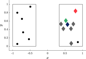
(a) $t=0$s

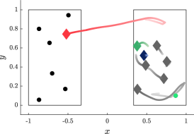
(b) $t=25$s

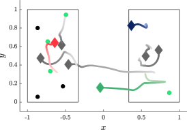
(c) $t=100$s

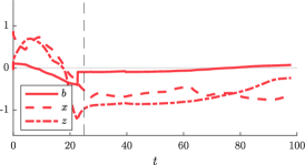
(d) Trajectory of the red agent.

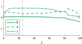
(e) Trajectory of the green agent.

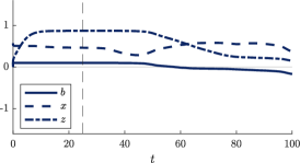
(f) Trajectory of the blue agent.

Figure 1: Application of the coupled NOD and physical dynamics model in (3) to multi-robot trash collection across two trash patches. LABEL:sub@subfig:dc_t_0-LABEL:sub@subfig:dc_t_150 show the positions of the robots (depicted as diamonds) at $t=0$, $t=25$ and $t=100$s. The patches boundaries are denoted by the rectangles and the uncollected (collected) trash pieces are shown in black (green). The bottom row shows the evolution of the opinion $z_{i}$, the position $x_{i}$ and input $b_{i}$, for the robots highlighted in red, blue, and green in the top row. Parameters: $q_{\min}=1.5$, $u=1.3$, $d=1$, $K_{z}=2$, $l=1$, $\sigma=0.1$, $k=10$, $K_{y}=0.15$.

II COUPLED NONLINEAR OPINION DYNAMICS AND PHYSICAL DYNAMICS

We consider an agent choosing between two spatially separated tasks, which requires an agent to travel when switching tasks, as illustrated in Fig. 1. Our framework couples the nonlinear opinion dynamics (NOD) model proposed in [1] and a model of the agent’s physical dynamics that determines the agent’s motion in executing its current task. The framework accounts for the agent’s physical limitations and the presence of obstacles or mechanical failures as well as environmental inputs. We review NOD in Section II-A. We define the physical dynamics in Section II-B and proposed threshold decision-making framework in Section II-C.

II-A Nonlinear Opinion Dynamics

We define the opinion $z\in\mathbb{R}$ of an agent as its preference over the two tasks. We refer to the region associated with task 1 (task 2) as patch 1 (patch 2). When $z>0\ (<0)$, the agent favors task 1 (task 2). If $z=0$, the agent is neutral or undecided about the tasks. The degree of commitment of the agent to a task is quantified by the magnitude $|z|$ of $z$.

We adopt the continuous-time multi-agent multi-option model presented in [1] to describe how a single agent’s opinion over two tasks varies over time:

$$\dot{z}=\tilde{f}(z):=-d\,z+uS\left(z\right)+b,$$ (1)

where $d>0$ is a damping coefficient, $u>0$ is a gain that represents the “attention” the agent pays to reinforcing its own opinion, and $b\in{\mathbb{R}}$ is a bias in favor of task 1 (task 2) if $b>0$ ($b<0$). We fix $d$ and let $u$ and $b$ be variable. $S:{\mathbb{R}}\rightarrow{\mathbb{R}}$ is an odd saturating function with $S(0)=0$, $S^{\prime}(0)=1$. For simulations we let $S(\cdot)=\tanh(\cdot)$.

One of the key features of (1), as discussed in [1], is that two isolated equilibria, corresponding to an opinion in favor of each of the options, arise through a bifurcation from the neutral equilibrium as a parameter, such as $u$, changes. When the agent is unbiased ($b=0$) the model (1) undergoes a supercritical pitchfork bifurcation at $u=u^{*}=d$ (as in Fig. 2 top left). For $u<u^{*}=d$, the opinion converges to the neutral state. When $u>u^{*}$, the neutral state becomes unstable, and two branches of locally exponentially stable opinionated equilibria appear. If the agent has a bias, i.e., $b>0$ ($b<0$), the bifurcation unfolds in the direction of the sign of $b$ (as in Fig. 2 top middle (right)). Therefore, for $b\neq 0$, when $u$ is near $u^{*}$ there is only one stable equilibrium $z^{*}$, with $\mathrm{sign}(z^{*})=\mathrm{sign}(b)$, and the agent’s decision-making becomes sensitive to the bias.

We leverage this feature of NOD for threshold decision-making by treating $b$ as a threshold variable. For a fixed value of $u>u^{*}$, as $b$ crosses 0 and $|b|$ becomes large enough so that $u$ is in the neighborhood of $u^{*}$ where there is only one stable equilibrium, the sign of $z^{*}$ changes and the agent switches tasks.

II-B Physical Agent Dynamics

Suppose without loss of generality that the patches for the two tasks have the same rectangular shape and are equidistant from the $x=0$ line in the two-dimensional Euclidean space. We take $l$ to be the distance from the outermost edge of the patche to the $x=0$ line. Without loss of generality, we assume that $l=1$. See Fig. 1 for an illustration of the patches in a multi-agent trash collection example, where each agent explores one of two patches at a given time as it searches and collects trash.

When an agent selects a task, it moves to the associated patch. It then randomly chooses from a uniform distribution a point $(r_{x},r_{y})$ in the patch. The waypoint the agent uses to carry out its task is defined as $(\bar{x}(z),\bar{y})$ where $\bar{y}=r_{y}$ and $\bar{x}(z)=\rho/l\tanh(kz)$ with $k>0$ and $\rho=|r_{x}|$. That is, only the $x$-coordinate of the waypoint depends on the agent’s opinion state $z$, as depicted in Fig. 1.

The physical dynamics evolve as a function of the opinion:

$$\dot{x} =K_{x}(\bar{x}(z)-x)=\tilde{h}(z,x)$$ (2a)

$$\dot{y} =K_{y}(\bar{y}-y).$$ (2b)

When the agent arrives at the waypoint, it chooses a new waypoint in the same fashion. The positive parameter $k$ determines the weight of the opinion on the physical dynamics. The term $\tanh(kz)$ ensures that when the agent’s opinion is sufficiently large in magnitude, the opinion dynamics do not impact the waypoint navigation within the patch, i.e., the agent moves very near to the random point $(r_{x},r_{y})$. $K_{x},K_{y}>0$ are proportional gains on the agent’s velocity.

II-C Coupled Opinion and Physical Dynamics

We propose a decision-making framework that takes the physical dynamics (2) into account in the opinion-forming process by coupling (1) and (2). Since the opinion $z$ affects only (2a), we omit (2b) in the coupled model. Let

$$\dot{z}=f(z,x):=\tilde{f}(z)-K_{z}\eta(z)\left(z-x\right)$$ (3a)

$$\dot{x}=h(z,x):=(1-\eta(z))\tilde{h}(z,x)-\eta(z)\left(x-z\right),$$ (3b)

where $\eta(z)=\exp(-z^{2}/2\sigma^{2})$, $\sigma>0$, sign$(z(0))=$ sign$(x(0))$, and $K_{z}>0$ is the coupling weight. The function $\eta(z)$ acts as a smooth switch between waypoint navigation and task switching. For $|z|$ large, $\eta(z)\approx 0$ and waypoint navigation is on so that the agent moves to the waypoint. For $|z|$ is small, $\eta(z)\approx 1$ and task switching is triggered such that the agent moves towards the origin. $\sigma$ determines how small $|z|$ needs to be to trigger a task switch.

To make the agent’s decision-making adaptive to the changes in the environment, bias $b$ and attention parameter $u$ can be tuned, as we show in Section III. The bias $b$ can be determined as the efficiency of the agent at the current task, as we demonstrate in Section IV.

III ANALYSIS OF DECISION-MAKING BEHAVIOR

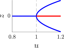
(a)

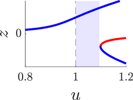
(b)

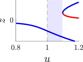
(c)

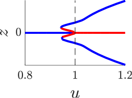
(d) $b=0$

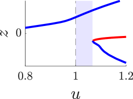
(e) $b>0$

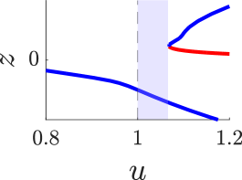
(f) $b<0$

Figure 2: Bifurcation diagrams of the NOD coupled to the physical dynamics of an agent (3). The top row illustrates the bifurcation diagrams for the parameter regime in which the system undergoes a symmetric supercritical pitchfork bifurcation and its unfolding. The bottom row shows the symmetric subcritical pitchfork bifurcation with a quintic stabilizing term and its unfolding. Blue lines show stable branches whereas red lines represent unstable branches. The vertical dashed line shows $u=u^{*}$. Regions with only one branch of equilibria for $u>u^{*}$ are shaded in light blue. Bifurcation diagrams generated with help of MatCont [17]. Parameters: $d=1$, $b\in\{0,\pm 0.2\}$, $K_{x}=3$, $k=10$, $\sigma=0.1$, $\rho=0.5$.

In Section III-A we show how threshold decision-making results through a bifurcation in the coupled dynamics (3). In Section III-B we show how the threshold decision-making is adaptive to physical constraints and environmental change.

III-A Threshold Decision-Making through a Bifurcation

In a nonlinear dynamical system, a bifurcation refers to a change in the number and/or stability of solutions as a parameter varies. The parameter and state value at which the change occurs is called a bifurcation point. The top left bifurcation diagram in Fig. 2 illustrates a supercritical pitchfork bifurcation at bifurcation point $(z,u)=(z^{*},u^{*})=(0,1)$ in which a (unique) stable equilibrium ($z=0$) becomes unstable and two symmetric equilibria are created. The bottom left diagram of Fig. 2 illustrates a subcritical pitchfork bifurcation at bifurcation point $(z,u)=(z^{*},u^{*})=(0,1)$, in which the two symmetric branches that emerge from the stable equilibrium at the bifurcation point are unstable and two further stable branches are created through saddle-node bifurcations. This is a subcritical pitchfork with a quintic stabilizing term bifurcation (see [18]).

We first show that, with $u$ as the bifurcation parameter, the dynamics (3) undergo either a supercritical pitchfork or a subcritical pitchfork with a quintic stabilizing term bifurcation. Observe that the neutral state $\left(z,x\right)=(0,0)$ is always an equilibrium of (3).

Lemma III.1

(Stability at Neutral Equilibrium) Let $b=0$. $J$ is the Jacobian of (3) evaluated at equilibrium $\left(z,x\right)=(0,0)$. Define $u^{*}=d$. Then, $\left(z,x\right)=(0,0)$ is locally exponentially stable for $0<u<u^{*}$ and unstable for $u>u^{*}$.

Proof:

The eigenvalues $\lambda_{1,2}$ of

$$J=\begin{bmatrix}(-d+u-K_{z})&K_{z}\\ 1&-1\end{bmatrix}$$

are $\lambda_{1,2}=\frac{1}{2}\left(-(a\pm\sqrt{\left(a\right)^{2}-4(d-u)}\right)$ where $a=d-u+K_{z}+1$. Then, $\operatorname{Tr}(J)=\lambda_{1}+\lambda_{2}=u-d-K_{z}-1$ and $\det(J)=\lambda_{1}\lambda_{2}=d-u$. For $0<u<u^{*}=d$, $\operatorname{Tr}(J)=\lambda_{1}+\lambda_{2}<0$ and $\det(J)=\lambda_{1}\lambda_{2}>0$, therefore $\lambda_{1},\lambda_{2}<0$ so the equilibrium $\left(z,x\right)=(0,0)$ is locally exponentially stable. For $u>u^{*}=d$, $\det(J)=\lambda_{1}\lambda_{2}<0$, therefore, $\lambda_{1}<0<\lambda_{2}$ so the equilibrium $\left(z,x\right)=(0,0)$ is unstable. ∎

To show the existence of a symmetric quintic pitchfork bifurcation at $\left(z,x\right)=(0,0)$, we first reduce the dynamics of (3) to a 1-D scalar differential equation. At equilibrium, $f(z,x)=0$ holds, so we can solve for $x$ in terms of $z$:

$$x=z+\left(\frac{dz-uS(z)+b}{K_{z}\eta(z)}\right).$$ (4)

Then, substituting (4) into $h(z,x)=0$ gives

$$\begin{split}(1-\eta\left(z\right))\tilde{h}\left(z,z+\left(\frac{dz-uS(z)+b}{K_{z}\eta(z)}\right)\right)+&\\ -\eta(z)\left(\frac{dz-uS(z)+b}{K_{z}\eta(z)}\right)&=\\ g(z,d,u,b,K_{x},K_{z},k,\sigma,\rho,l)&=0\end{split}$$ (5)

a scalar equilibrium bifurcation problem.

Theorem III.2

(Decision-Making Through Bifurcation) Consider the equilibrium bifurcation problem (5) with $u$ as the bifurcation parameter and $b=0$. Suppose that $-2d/K_{z}-3K_{x}(1-k\rho/l)/\sigma=0$. In a neighborhood of ${\left(u,z\right)}=(u^{*},0)$, the bifurcation problem is strongly equivalent (in the sense of [19, Definition VI.2.5]) to the quintic pitchfork bifurcation problem $-z^{5}+(u-u^{*})z=0$, where $z$ is the state and $u$ the bifurcation parameter. If $-2d/K_{z}-3K_{x}(1-k\rho/l)/\sigma\neq 0$, at the equilibrium ${\left(z,x\right)}=(0,0)$ with $u^{*}=d$, the quintic pitchfork bifurcation unfolds into either a supercritical pitchfork bifurcation if $-2d/K_{z}-3K_{x}(1-k\rho/l)/\sigma<0$ or into a subcritical pitchfork bifurcation with a quintic stabilizing term if $-2d/K_{z}-3K_{x}(1-k\rho/l)/\sigma>0$.

Proof:

For $b=0$, the bifurcation problem (5) is $Z_{2}$ symmetric with respect to $z\mapsto-z$ because $g(-z,d,u,0,K_{x},K_{z},k,\sigma,\rho,l)=-g(z,d,u,0,K_{x},K_{z},k,\sigma,\rho,l)$. Let $g_{z}$ denote the partial derivative of $g$ with respect to $z$ and similarly for higher-order and mixed derivatives. Following the recognition problem in [19, Proposition VI.2.14], we compute

$$g(z^{*},d,u^{*},0,K_{x},K_{z},k,\sigma,\rho,l)=0,$$ (6)

$$g_{z}(z^{*},d,u^{*},0,K_{x},K_{z},k,\sigma,\rho,l)=0,$$ (7)

$$\begin{split}&g_{zzz}(z^{*},d,u^{*},0,K_{x},K_{z},k,\sigma,\rho,l)\\ &=-\frac{2d}{K_{z}}-\frac{3K_{x}}{\sigma}\left(1-\frac{k\rho}{l}\right)=0,\end{split}$$ (8)

$$\begin{split}&g_{zzzzz}(z^{*},d,u^{*},0,K_{x},K_{z},k,\sigma,\rho,l)\\ &=-\frac{1}{K_{z}\sigma^{2}}\left(20K_{x}K_{z}k^{3}\sigma\rho/l+15K_{x}K_{z}k\rho/l\right.\\ &\left.-16d\sigma^{2}+20K_{x}d\sigma-15K_{x}K_{z}\right)<0\end{split}$$ (9)

$$g_{u}(z^{*},d,u^{*},0,K_{x},K_{z},k,\sigma,\rho,l)=0,$$ (10)

$$g_{zu}(z^{*},d,u^{*},0,K_{x},K_{z},k,\sigma,\rho,l)=\frac{1}{K_{z}}.$$ (11)

Since $g_{zzz}(z^{*},d,u^{*},0,K_{x},K_{z},k,\sigma,\rho,l)=0$, $g_{zzzzz}(z^{*},d,u^{*},0,K_{x},K_{z},k,\sigma,\rho,l)<0$, and $g_{zu}(z^{*},d,u^{*},0,K_{x},K_{z},k,\sigma,\rho,l)>0$, by [19, Proposition VI.2.14], the symmetric quintic bifurcation recognition problem is complete.

If $-2d/K_{z}-3K_{x}(1-k\rho/l)/\sigma\neq 0$, then the cubic term $g_{zzz}\neq 0$ in (8). Since the cubic term is non-zero, then by [19, Theorem VI.3.3], the quintic pitchfork unfolds into a supercritical pitchfork if the cubic term is negative or into a subcritical pitchfork bifurcation with a quintic stabilizing term if the cubic term is positive. ∎

Theorem III.2 reveals that for $u>u^{*}$, threshold decision-making can be implemented by varying $b$ like in the uncoupled NOD. This is because it follows from unfolding theory for a pitchfork bifurcation [19, Ch. I] that when $b\neq 0$, the symmetric pitchfork unfolds such that only one solution, predicted by the sign of $b$, is stable close to the bifurcation point. The top row of Fig. 2 illustrates the bifurcation diagrams for the parameters that satisfy the condition for a supercritical pitchfork and its unfolding. Similarly, the bottom row of Fig. 2 shows the bifurcation diagram for parameters that satisfy the condition for the subcritical pitchfork with quintic stabilizing term. Note that in both the subcritical and supercritical cases, for $u>u^{*}$, there is only one branch of equilibria in the shaded regions.

Since we are interested in varying $b$ for threshold decision-making, we now investigate how the system bifurcates when $b$ is the bifurcation parameter.

Proposition III.3

(Existence of Saddle Node Bifurcations) Consider the equilibrium bifurcation problem (5) with $b$ as the bifurcation parameter and $u>u^{*}$. For $u$ close to $u^{*}$, as $b$ varies, there exist two saddle node bifurcations, one at $(z_{1}^{*},b_{1}^{*})$ with $z_{1}>0>b_{1}$ and one at $(z_{2}^{*},b_{2}^{*})$ with $z_{2}<0<b_{2}$.

Proof:

Obtaining a closed form solution for $(z_{1}^{*},b_{1}^{*})$, $(z_{2}^{*},b_{2}^{*})$ is non-trivial, so we instead examine the normal forms of the supercritical pitchfork ($\dot{z}=-z^{3}+(u-d)z+b$), the quintic pitchfork ($\dot{z}=-z^{5}+(u-d)z+b$) and the subcritical pitchfork with a quintic stabilizing term ($\dot{z}=-z^{5}+z^{3}+(u-d)z+b$). By Proposition III.2, the bifurcation problem near $u=u^{*}=d$ is strongly equivalent to one of the three pitchfork bifurcation problems.

For the supercritical pitchfork case, let $\hat{g}(z,b,u,d)=-z^{3}+(u-d)z+b$. Following the recognition problem in [19, Theorem IV.2.1]), we seek $z^{*}$, $u^{*}$ such that

$$\hat{g}(z^{*},b^{*},u,d)=-z^{3}+(u-d)z+b=0$$ (12)

$$\hat{g}_{z}(z^{*},b^{*},u,d)=-3z^{2}+(u-d)=0$$ (13)

$$\hat{g}_{zz}(z^{*},b^{*},u,d)=-6z\neq 0$$ (14)

$$\hat{g}_{b}(z^{*},b^{*},u,d)\neq 0.$$ (15)

We first solve for $z^{*}$ in (13). Then, we plug $z^{*}$ into (12) to solve for $b^{*}$. Note that $u>d$. Then,

$$(z_{1}^{*},b_{1}^{*})=\left(\sqrt{\frac{u-d}{3}},-2\left(\frac{u-d}{3}\right)^{\frac{3}{2}}\right)$$ (16)

$$(z_{2}^{*},b_{2}^{*})=\left(-\sqrt{\frac{u-d}{3}},2\left(\frac{u-d}{3}\right)^{\frac{3}{2}}\right).$$ (17)

Note that conditions (15) and (14) are satisfied since $\hat{g}_{b}=1\neq 0$ and $z$. Then, for both saddle points, $z^{*},b^{*}\neq 0$ and sign$(z^{*})$ = -sign$(b^{*})$. The same process can be repeated for the quintic pitchfork and subcritical pitchfork cases. In both instances, we can verify that there are two saddle points that satisfy $z^{*},b^{*}\neq 0$ and sign$(z^{*})$ = -sign$(b^{*})$. ∎

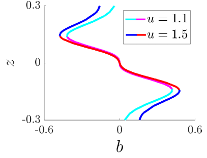
(a)

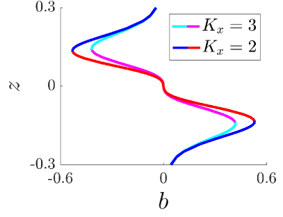
(b)

Figure 3: Bifurcation diagrams of NOD coupled to physical dynamics of an agent (3) illustrating how $u$ and $K_{x}$ effectively change the task switching threshold by changing the size of the bistable region. Left: bifurcation diagram corresponding to two different values of $u$. Right: bifurcation diagram corresponding to two different values of $K_{x}$. Blue lines show stable branches of equilibria. Red and magenta lines show unstable branches of equilibria. Bifurcation diagrams generated with MatCont [17]. Parameters: $d=1$, $k=10$, $\sigma=0.1$, $\rho=0.5$, Left: $K_{x}=3$, Right: $u=1.1$.

The saddle nodes serve as the threshold for which the agent switches tasks. As seen in Fig. 3, if the agent starts at the positive branch of stable equilibria, once $b$ is sufficiently negative (i.e. crosses $b_{1}^{*}$), the negative branch becomes the only stable branch. Similarly, if the agent starts at the negative branch, once $b$ is sufficiently positive (i.e. crosses $b_{2}^{*}$), the positive branch becomes the only stable one. Hence, for threshold decision-making, the saddle nodes act like thresholds with $b$ as the threshold parameter.

III-B Threshold Decision-Making Adaptive to Environmental Changes and Physical Constraints

We now show how the system adapts to the agent’s physical constraints and how tuning a single parameter allows the system to adapt to changing environments.

Theorem III.4

(Adaptability to the Environment Through Saddle Node Bifurcations) Varying the parameter $u$ changes the size of the bistable region by changing the location of the saddle points $(z_{1}^{*},b_{1}^{*})$ and $(z_{2}^{*},b_{2}^{*})$. Larger $u$ corresponds to a larger bistable region (i.e. higher input is required for switching) and smaller $u$ corresponds to a smaller bistable region (i.e. lower input is required for switching).

Proof:

At the saddle node points $(z_{1}^{*},b_{1}^{*})$ and $(z^{*}_{2},b^{*}_{2})$, $g(z_{1}^{*},d,u,b_{1}^{*},K_{x},K_{z},k,\sigma,\rho,l)=0$ and $g(z_{2}^{*},d,u,b_{2}^{*},K_{x},K_{z},k,\sigma,\rho,l)=0$. Therefore, by the Implicit Function Theorem, the change in location of the saddle points with respect to $u$ can be expressed as

$$\frac{\partial b^{*}}{\partial u}=-\left(\frac{\partial g}{\partial b}\right)^{-1}\frac{\partial g}{\partial u}=-S(z)$$ (18)

since

$$\frac{\partial g}{\partial b}=\frac{\left(K_{x}\left(\frac{1}{\eta(z)}-1\right)+1\right)}{K_{z}}$$ (19)

$$\frac{\partial g}{\partial u}=S(z)\frac{\left(K_{x}\left(\frac{1}{\eta(z)}-1\right)+1\right)}{K_{z}}\,.$$ (20)

From Proposition III.3, $z^{*}_{1}>0>z^{*}_{2}$ and $b^{*}_{1}<0<b^{*}_{2}$, so from (18), we have $\partial b_{1}^{*}/{\partial u}<0$ and $\partial b_{2}^{*}/{\partial u}>0$. Therefore, as $u$ increases, the saddle node points moves away from the origin. ∎

Proposition III.5

(Adaptability to Physical Constraints Through Saddle Node Bifurcations) Varying the parameter $K_{x}$ changes the size of the bistable region by changing the location of the saddle points $(z_{1}^{*},b_{1}^{*})$ and $(z_{2}^{*},b_{2}^{*})$. Larger $K_{z}$ corresponds to a smaller bistable region (i.e. lower input is required for switching) and smaller $K_{x}$ corresponds to a larger bistable region (i.e. higher input is required for switching).

Proof:

The proof follows the same method as the one presented in Theorem III.4, except with respect to $K_{x}$ instead of $u$. Therefore, the change in location of the saddle points with respect to $K_{x}$ can be expressed as

$$\begin{split}\frac{\partial b^{*}}{\partial K_{x}}&=-\left(\frac{\partial g}{\partial b}\right)^{-1}\frac{\partial g}{\partial K_{x}}.\\ &=\left(\frac{K_{z}(\eta(z)-1)}{K_{x}\left(\frac{1}{\eta(z)}-1\right)1}\right)\left(\frac{\rho\tanh(kz)}{l}\right.\\ &+\left.\frac{1}{K_{z}\eta(z)}\left(b-dz+uS(z)-K_{z}z\eta(z)\right)\right)\,.\end{split}$$ (21)

Since determining the sign of $\frac{\partial b^{*}}{\partial K_{x}}$ is non-trivial, we examine the evolution of $\frac{\partial b^{*}}{\partial K_{x}}$ as a function of $z$ for small values of $b^{*}$. As seen in Fig. 4, we have $\partial b_{1}^{*}/{\partial K_{x}}<0$ and $\partial b_{2}^{*}/{\partial K_{x}}>0$ for $z^{*}_{1}>0>z^{*}_{2}$ and $b^{*}_{1}<0<b^{*}_{2}$. Therefore, as $K_{x}$ increases, the saddle node points moves towards the origin. ∎

Theorem III.4 and Proposition III.5 imply that the decision-making threshold, which is given by the location of the saddle nodes, can be modulated by $K_{x}$ and $u$. Fig. 3 illustrates how changing both of these parameters have the same global effect: changing the size of the size of the bistable region which effectively changes the decision-making threshold. On the left, we see that increasing $u$ increases the switching threshold, while on the right we see that increasing $K_{x}$, decreases the switching threshold. We take advantage of these behaviors in the applications of this decision-making model to task allocation to allow agents to adapt to their environment by varying $u$ and to their physical constraints by varying $K_{x}$.

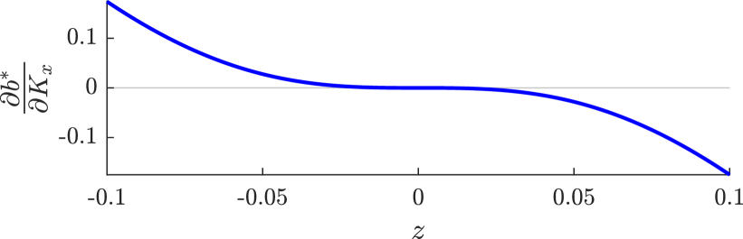
Figure 4: Evolution of $\partial b^{*}/\partial K_{x}$ as a function of $z$. Parameters: $d=1$, $u=1.2$, $K_{x}=0.05$, $k=10$, $\sigma=0.1$, $\rho=0.8$.

IV APPLICATIONS TO TASK ALLOCATION

We illustrate how the proposed threshold decision-making and physical dynamics model can be used in multi-robot task allocation applications to allow robots to individually adapt to changing environments, how it can accommodate the robots’ physical constraints, and how it can be used to reduce congestion in regions with clusters of robots (i.e., a large number of robots close together).

We study a multi-robot trash collection problem in which trash-collecting robots with low sensory capabilities use the decision-making model in (3) to select which patch to search and collect trash from based on perceived efficiency of the currently selected patch. In this dynamic task allocation problem, patch resources change as a result of robots picking-up the trash and because trash can be added to the patches. We consider the efficiency $q\in{\mathbb{R}}_{+}$ of a robot to be given by the ratio of perceived resource abundance to energy spent,

$$q=\frac{\mbox{\# of trash pieces collected in the patch}+q_{0}}{\mbox{distance travelled within patch}+\epsilon},$$ (22)

where the constant $q_{0}>0$ ensures that $q>0$ and $\epsilon>0$ ensures that $q$ is always defined. In practice, $q_{0}>>\epsilon$.

We can calculate the appropriate input $b$ to the decision making in model (3) as a function of the efficiency:

$$b(q)=s(\tanh(q)-\tanh(q_{\min})),$$ (23)

where the value of $q$ is reset and $s$ changes sign whenever a robot enters a patch after switching. When the robot enters patch 1, $s=1$, and when the robot enters patch 2, $s=-1$. In that way, when $q$ falls below $q_{\min}$, the $b$ makes the robot start favoring the other patch.

Adaptability to Environmental Changes

Our approach provides flexibility by allowing robots to adapt their decision-making in response to environment changes, such as changes to global resource availability. These changes can be captured by varying the value of $u$ based on robot measurements or a model of how the resources are changing.

See Fig. 5 where trash is added to patch 2, and the red square-shaped robot receives a signal to increase $u$, effectively increasing its switching threshold. Then, for the same input, the red square-shaped robot switches patches before the blue triangle-shaped robot and heads to the patch which now has more abundant resources.

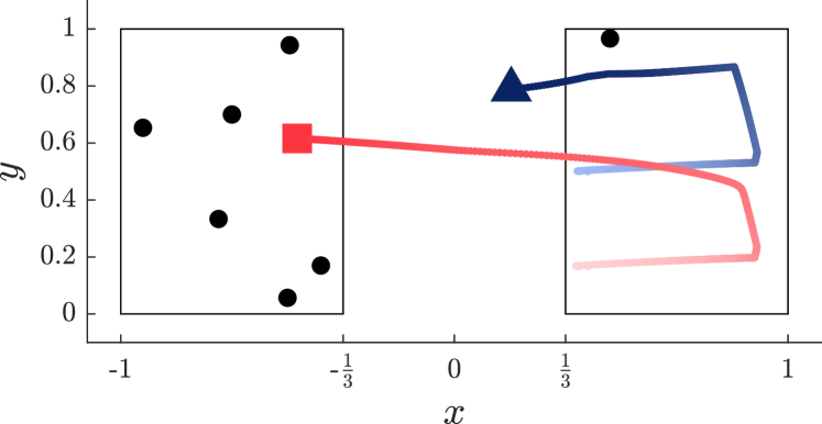
(a)

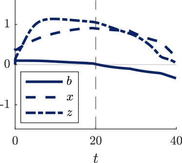
(b)

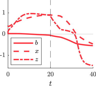
(c)

Figure 5: Two robots, depicted as a red square and a blue triangle, collecting trash (black circles) across two trash patches (black rectangles) adapt to environmental changes. At $t=20$, the red robot receives a signal from the environment to decrease $u$ thus increasing its switching threshold. Top: spatial trajectory of the two robots. Bottom: time trajectory of the opinion $z$, the position $x$ and input $b$ of each robot. Parameters: $q_{\min}=1.5$, $d=1$, $K_{z}=2$, $l=1$, $\sigma=0.1$, $k=10$, $K_{y}=0.15$, $K_{x}=0.15$. Before $t=20$, red, blue robots: $u=1.3$. After $t=20$, red robot: $u=1.05$, blue robot: $u=1.3$.

Emergent Explore-Exploit Behavior with Heterogeneous Robots

The ability of a robot to perform a task can be influenced by the robots’s physical constraints. Seemingly homogeneous robots may still experience some level of heterogeneity since many factors can affect their performance, e.g. battery charge levels, battery age, CPU temperatures, motor strain, or payload weight. Additionally, for some task allocation applications, a heterogeneous group of robots can be more advantageous. A smaller and faster robot could be better at exploring the environment while a larger and slower one could be better at carrying heavier payloads.

The coupling term in our decision-making model makes the model adaptive to the physical constraints of the robot. We observe that for a group of heterogeneous robots, this feature leads to emergent explore-exploit behavior. As seen in Fig. 6, given the same input, the faster red squared-shaped robot switches before the blue triangle-shaped robot. Therefore, the faster robot presents a more exploratory behavior while the slower one presents a more exploitative behavior.

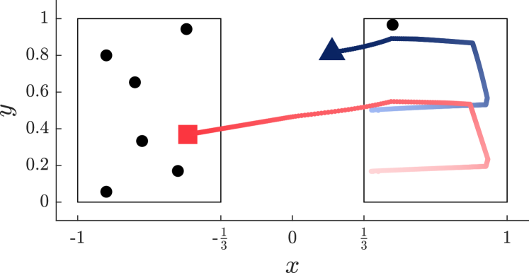
(a)

(b)

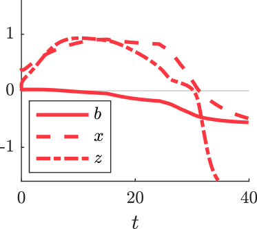
(c)

Figure 6: Two robots with different physical constraints, depicted as a red square and a blue triangle, collecting trash (black circles) across two trash patches (black rectangles). The red robot is faster than the blue robot. Top: spatial trajectory of the two robots. Bottom: time trajectory of the opinion $z$, the position $x$ and input $b$ of each robot. Parameters: $q_{\min}=1.5$, $u=1.3$, $d=1$, $K_{z}=2$, $l=1$, $\sigma=0.1$, $k=10$, $K_{y}=0.15$, red robot: $K_{x}=0.15$. blue robot: $K_{x}=0.11$.

Declustering Behavior

In crowded regions, the congestion can considerably slow down robots for extended periods of time, which prevents them from performing their assigned tasks.

Fig. 1 illustrates how our model relieves traffic congestion. Some of the robots are initially clustered in the center of patch. The control barrier function based collision avoidance algorithm [20] used slows them down by effectively changing the value of $K_{x}$. The robots that are not near the cluster are free to move faster, so their switching threshold is higher. This leads them to switch more quickly leaving the patch less crowded. Eventually, the cluster disappears. Note that the blue robot which was slowed down the most due to being in the center of the cluster is the last robot to switch patches since it has the lowest threshold value.

V DISCUSSION AND FINAL REMARKS

We have presented a threshold decision-making framework that allows for flexible task allocation for spatial task applications through the coupling of opinion dynamics to the physical dynamics of the robot. In future work, we aim to generalize the results in III and III-B to non-symmetric patches, extend the analysis to the multi-option dynamics of [1] and implement the algorithm on physical robots.

References

- [1] A. Bizyaeva, A. Franci, and N. E. Leonard, “Nonlinear opinion dynamics with tunable sensitivity,” IEEE Transactions on Automatic Control, vol. 68, no. 3, pp. 1415–1430, 2023.
- [2] C. Cathcart, M. Santos, S. Park, and N. E. Leonard, “Proactive opinion-driven robot navigation around human movers,” in IEEE/RSJ International Conference on Intelligent Robots and Systems (IROS’23), 2023.
- [3] S. Park, A. Bizyaeva, M. Kawakatsu, A. Franci, and N. E. Leonard, “Tuning cooperative behavior in games with nonlinear opinion dynamics,” IEEE Control Systems Letters, vol. 6, pp. 2030–2035, 2022.
- [4] H. Hu, K. Nakamura, K.-C. Hsu, N. E. Leonard, and J. F. Fisac, “Emergent coordination through game-induced nonlinear opinion dynamics,” in IEEE Conference on Decision and Control, 2023.
- [5] A. Bizyaeva, G. Amorim, M. Santos, A. Franci, and N. E. Leonard, “Switching transformations for decentralized control of opinion patterns in signed networks: Application to dynamic task allocation,” IEEE Control Systems Letters, vol. 6, pp. 3463–3468, 2022.
- [6] B. P. Gerkey and M. J. Matarić, “A formal analysis and taxonomy of task allocation in multi-robot systems,” The International Journal of Robotics Research, vol. 23, no. 9, pp. 939–954, 2004.
- [7] M. B. Dias, “Traderbots: A new paradigm for robust and efficient multirobot coordination in dynamic environments,” Ph.D. dissertation, Carnegie Mellon University, Pittsburgh, PA, January 2004.
- [8] M. Dias, R. Zlot, N. Kalra, and A. Stentz, “Market-based multirobot coordination: A survey and analysis,” Proceedings of the IEEE, vol. 94, no. 7, pp. 1257–1270, 2006.
- [9] L. Lin and Z. Zheng, “Combinatorial bids based multi-robot task allocation method,” in Proceedings of the 2005 IEEE International Conference on Robotics and Automation, 2005, pp. 1145–1150.
- [10] W. Saad, Z. Han, T. Basar, M. Debbah, and A. Hjorungnes, “Hedonic coalition formation for distributed task allocation among wireless agents,” IEEE Transactions on Mobile Computing, vol. 10, no. 9, pp. 1327–1344, 2011.
- [11] I. Jang, H.-S. Shin, and A. Tsourdos, “Anonymous hedonic game for task allocation in a large-scale multiple agent system,” IEEE Transactions on Robotics, vol. 34, no. 6, pp. 1534–1548, 2018.
- [12] S. Park, Y. D. Zhong, and N. E. Leonard, “Multi-robot task allocation games in dynamically changing environments,” in IEEE International Conference on Robotics and Automation (ICRA), Xi’an, China, 2021, pp. 8678–8684.
- [13] M. J. Krieger and J.-B. Billeter, “The call of duty: Self-organised task allocation in a population of up to twelve mobile robots,” Robotics and Autonomous Systems, vol. 30, no. 1, pp. 65–84, 2000.
- [14] W. Agassounon and A. Martinoli, “Efficiency and robustness of threshold-based distributed allocation algorithms in multi-agent systems,” ser. AAMAS ’02. New York, NY, USA: Association for Computing Machinery, 2002, p. 1090–1097.
- [15] E. Castello, T. Yamamoto, F. Dalla Libera, W. Liu, A. Winfield, Y. Nakamura, and H. Ishiguro, “Adaptive foraging for simulated and real robotic swarms: the dynamical response threshold approach,” Swarm Intelligence, vol. 10, pp. 1–31, 03 2016.
- [16] N. Kalra and A. Martinoli, Comparative Study of Market-Based and Threshold-Based Task Allocation, 06 2007, pp. 91–101.
- [17] A. Dhooge, W. Govaerts, I. Kouznetsov, H. Meijer, and B. Sautois, “New features of the software matcont for bifurcation analysis of dynamical systems.” Mathematical and Computer Modelling of Dynamical Systems, vol. 14, no. 1/2, pp. 147–175, 2008.
- [18] S. H. Strogatz, Nonlinear Dynamics and Chaos: With Applications to Physics, Biology, Chemistry and Engineering. Westview Press, 2000.
- [19] M. Golubitsky and D. G. Schaeffer, Singularities and Groups in Bifurcation Theory, ser. Applied Mathematical Sciences. New York, NY: Springer-Verlag, 1985, vol. 51.
- [20] L. Wang, A. D. Ames, and M. Egerstedt, “Safety barrier certificates for collisions-free multirobot systems,” IEEE Transactions on Robotics, vol. 33, no. 3, pp. 661–674, 2017.