Precise Phase Error Rate Analysis for Quantum Key Distribution with Phase Postselection
Abstract
Quantum key distribution (QKD) stands as a pioneering method for establishing information-theoretically secure communication channels by utilizing the principles of quantum mechanics. In the security proof of QKD, the phase error rate serves as a critical indicator of information leakage and directly influences the security of the shared key bits between communicating parties, Alice and Bob. In estimating the upper bound of the phase error rate, phase randomization and subsequent postselection mechanisms serve pivotal roles across numerous QKD protocols. Here we make a precise phase error rate analysis for QKD protocols with phase postselection, which helps us to accurately bound the amount of information an eavesdropper may obtain. We further apply our analysis in sending-or-not-sending twin-field quantum key distribution (SNS-TFQKD) and mode-pairing quantum key distribution (MP-QKD). The simulation results confirm that our precise phase error analysis can noticeably improve the key rate performance especially over long distances in practice. Note that our method does not require alterations to the existing experimental hardware or protocol steps. It can be readily applied within current SNS-TF-QKD and MP-QKD for higher key rate generation.
I Introduction
Quantum key distribution (QKD) [1, 2] provides the unconditional secure keys, which can not be break even if the eavesdropper Eve has unlimited computing resources, between two remote parties by exploiting the fundamental properties of quantum physics. During the past four decades, QKD has achieved great development in terms of security [3, 4, 5, 6, 7, 8, 9, 10, 11, 12, 13] and practicality [14, 15, 16, 17, 18, 19, 20, 21, 22, 23, 24, 25, 26, 27, 28, 29, 30, 31, 32, 33]. The decoy-state method [14, 15, 16] allows QKD systems to utilize coherent optical sources, diverging from the standard single-photon source BB84 protocol. This adaptation renders practical QKD systems resilient against photon number splitting (PNS) attacks, significantly enhancing both the secure key rate and the achievable communication distance. Measurement-device-independent (MDI) QKD protocol [17] (see also [18]) designates the measurement party as an untrusted intermediary situated within the channel, thereby making the key bits shared between two communication parties immune to all detector side attacks. However, due to the inherent transmission loss in the channel, the key rate performance in previous QKD is naturally constrained by the PLOB rate-transmittance bound [34] (see also the TGW bound [35]). The pursuit of longer communication distance and higher secure key rate is the central issue of practical QKD. Based on the simple and promising MDI-QKD structure, twin-field quantum key distribution (TF-QKD) [20] and mode-pairing quantum key distribution (MP-QKD) [31] (also named asynchronous-MDI-QKD [32]) were proposed to break the PLOB bound without quantum repeaters in recent years. Currently, these special variants substantially extend the point-to-point transmission distance, significantly advancing the practicality of QKD for longer-distance applications.
Roughly speaking, most QKD protocols consist of code mode and decoy mode. The communicating parties Alice and Bob generate the raw keys in the code mode and disclose a part of raw keys to estimate the bit error rate for error correction step. The key information leakage of QKD can be bounded by the so-called phase error rate [4, 5, 7], which can be estimated in the decoy mode. From the perspective of the equivalent entanglement-based scheme for the actual QKD protocol, the key is obtained by measuring the bipartite auxiliary qubits AB in the basis. The phase error rate is usually defined as the bit error rate of qubits AB in the basis. Nevertheless, we find that in certain QKD protocols with phase postselection, the definition of phase error rate occurs not in the X basis but rather in the conjugate basis . The distinct definitions of phase error rate across various conjugate bases commonly yield differing values, which prompts us to make a precise phase error rate analysis.
Based on the above idea, we propose a precise phase error rate analysis in this paper to further reduce the lower bound of phase error rate. Our method demonstrates noticeable enhancements in key rate performance for several QKD protocols with phase postselection, such as sending-or-not-sending twin-field quantum key distribution (SNS-TFQKD) [22] and MP-QKD.
We structure the remainder of this paper as follows. In Sec.II, we introduce a general equivalent entanglement-based scheme applicable to certain MDI-QKD variants and perform the precise phase error rate analysis. In Sec.III, we give the security proof for SNS-TF-QKD based on the equivalent entanglement-based scheme and obtain a precise phase error rate from the previously established formula. Our simulations demonstrate the noticeable enhancement achieved by our method in practical AOPP-SNS-TFQKD protocol. Additionally, we provide a brief overview of MP-QKD and showcase the improvements facilitated by our approach. Finally, a conclusion is given and we expect our method can be used in current AOPP-SNS-TFQKD and MP-QKD protocols.
II The precise phase error analysis
We first consider the following equivalent entanglement-based scheme for certain MDI-QKD variants in fig.1.
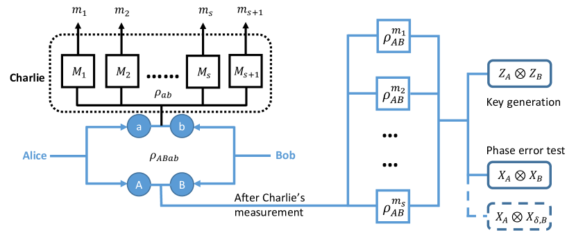
The communicating parties Alice and Bob prepare the ancillary qubit particles , and the signal particles , in a joint quantum state . The signal particles and are sent to untrusted party Charlie through an untrusted channel. Charlie measures the received signal states and announces the measurement outputs ( and ). Without loss of generality, we can introduce a positive operator-valued measure (POVM), which is a set of positive semi-definite Hermitian matrices acting on state associated with the outcomes , to denote the Charlie’s measurement and channel transmission effects. So the probability of the outcome is . After Charlie’s measurement and announcing the outcome , the ancillary bipartite qubits collapse into the normalized quantum state . Note that the measurement outcome denotes an invalid event, which is not used to generate keys. For the ancillary bipartite qubits (), Alice and Bob both measure them in the basis to obtain the key bits or measure them in the basis for phase error test. If Alice still measures her ancillary qubit in the basis but Bob measures his ancillary qubit in the basis, it can still be used for phase error test. In fact, we can introduce a unitary operator for Bob’s qubit B to convert the ancillary bipartite qubits to where and . As discussed in ref.[33], this unitary operator has no physical effects on the key bits generation and Eve’s potential system. It is obvious that the measurement output for in the and basis can be defined as the phase error. So we conclude that the phase error rate can be obtained by measuring the in the and basis due to the fact that such measurement output is equivalent to measuring in the and basis.
In fact, we can separately define the phase error rates of the key bits under every effective announcement by Charlie. That means we can classify the key bits into classes according to the announced outputs by Charlie. We denote the phase error rate of under the and basis as and under the and basis as . We will estimate the upper bound on given below.
For the given ancillary bipartite qubits , Alice first measures her local qubit in the basis and obtain the state with probability and with probability (). Bob also measures his local qubit in the basis. Given Alice’s output , we can assume that Bob obtains the state with probability and with probability . Given Alice’s output , we assume that Bob obtains the state with probability and with probability . Here, we have the phase error rate
| (1) |
Given Alice’s output , Bob’s density matrix is
| (2) |
where is a complex number, is the complex conjugate of . If Bob measures in the basis and defines the output as the error event, the error rate is
| (3) |
where is the real part of the complex number . Given Alice’s output , Bob’s density matrix is
| (4) |
where is a complex number, is the complex conjugate of . If Bob measures in the basis and defines the output as the error event, the error rate is
| (5) |
So the phase error rate under the and basis is
| (6) |
where . Note that is independent of .
In most practical MDI-QKD variants, we do not consider the phase error rates under different Charlie’s announcements but define only one phase error rate for all key bits. We assume that the probability of effective events announced by Charlie in an effective round is (). So the total phase error rate under the and basis is
| (7) |
and the total phase error rate under the and basis is
| (8) |
We find that the phase error rate in some certain QKD variants with phase postselection is defined as (), which is easily estimated by the decoy-state analysis. In fact, and have the following correlation
| (9) |
where . So, we can estimate the precise phase error rate by the previous given phase error rate
| (10) |
where is the upper bound of previous loose phase error rate estimated by the decoy-state analysis. Note that our analysis is applicable to the finite-key regime as long as the previous loose phase error rate is also for the finite-key case.
III Some QKD with phase postselection applicable to our method
We find some QKD protocols with phase postselection applicable to our precise phase error rate analysis. We aim to implement our method within SNS-TFQKD and MP-QKD protocols, simulating its potential enhancements.
III.1 apply our method to SNS-TFQKD
The SNS-TFQKD protocol, introduced by Wang et al. in 2018, has emerged as a prominent TF-QKD protocol in current practice. In code mode, Alice (Bob) generates a key bit 1 (0) with a probability of while sending a phase-randomized coherent state. Conversely, she (he) generates a key bit 0 (1) with a probability of and does not send anything. We give the equivalent entanglement-based scheme as follows:
| (11) |
where and denote the local auxiliary qubits which are used to generate the key between Alice and Bob, denotes the vacuum state, denotes the phase-randomized coherent state sent by Alice (Bob), is the Poisson distribution with mean photon number , and () is the random phase.
In a round of code mode in SNS-TFQKD, the key bit shared between Alice and Bob when one side sends nothing and the other side happens to send out the single-photon pulse is defined as the untagged bit [22]. Only the untagged bits are deemed as genuinely valid coded bits, originating from the partial quantum state within the corresponding entanglement-based scheme.
| (12) |
where is the single-photon state when Alice (Bob) sends the coherent state. In fact, the relative phase between and plays no roles in the results of the measurement for generating the secure key and Eve’s potential system. As the method proposed in ref.[33], we can introduce a unitary operation to the bipartite auxiliary qubits AB before the measurement on them, where and . This unitary operation can be achieved by constructing a hypothetical private channel through which Alice and Bob can share phase information and . So the quantum state can take the following equivalent form
| (13) |
We can reformulate in the and basis as
| (14) |
This indicates that the phase error rate defined in the and basis is related to the yields of the quantum states and .
In the decoy mode of SNS-TFQKD, Alice and Bob prepare and send the phase-randomized coherent state with intensity to Charlie. After Charlie’s measurement and announcement, Alice and Bob disclose the phases and of each pulse and post-select the instances that and for phase error rate estimation [36]. When the phase difference between Alice and Bob is or , they can estimate the phase error rate as depicted in (8). So our precise phase error analysis is adapted to SNS-TFQKD protocol. In the decoy mode, ref.[36] uses the round that Alice and Bob both send the coherent state with intensity to estimate the phase error rate in (9) as
| (15) |
where is the error click ratio of the instances that Alice and Bob both send the coherent pulse with intensity and their phase difference meets the post-selection condition: or [36], is the counting rate of vacuum sate and is the lower bound of the counting rate of single-photon state. So the precise phase error rate is
| (16) |
We use this precise phase error analysis in the practical AOPP-SNS-TFQKD protocol [28, 37, 29] and simulate the original AOPP-SNS-TFQKD and our improved protocol in fig.2.
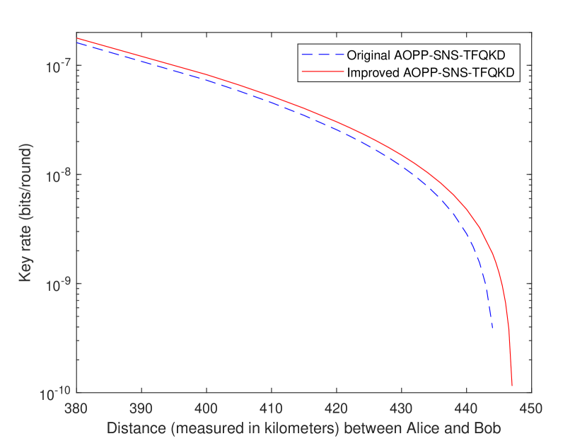
We use the same finite-key analysis and linear simulation model mentioned in ref.[29]. We set the total sending pulse as , the misalignment error as 5%, the dark count rate as , the fiber loss coefficient as , the photon detection efficiency as 30%, the error correction inefficiency as and the failure probability when calculating the effect of statistical fluctuation as . Furthermore, we achieve a security level of in the sense of composable security against coherent attacks. The simulation results indicate a key rate improvement of over 10% for distances beyond , accompanied by an extended maximum achievable distance of . These findings affirm the practical effectiveness of our precise phase error analysis in noticeably enhancing the key rate performance.
III.2 apply our method to MP-QKD
The specific process of MP-QKD protocol and the security proof in the finite-key regime based on the equivalent entanglement-based scheme have been thoroughly discussed in ref.[33]. Here, we provide a brief overview of the coded quantum states sent by Alice and Bob and directly show the equivalent entanglement-based scheme.
In each round of MP-QKD, Alice (Bob) randomly sends the phase-randomized coherent pulses with intensity and and the vacuum state with probabilities , and to untrusted node Charlie for interference measurement. Only the rounds where only detector L or R clicks are kept for subsequent step. In the post-processing step, Alice and Bob choose two rounds in the maximal pairing interval to form the effective event pair. We denote the intensity in the first and second round of the effective event pair as and . Only those pairs in which vacuum states are paired with weak coherent states are used for key generation. Alice sets her key bit to 0 if or 1 if . Bob sets her key bit to 0 if or 1 if . Similar to SNS-TFQKD, only the key bit when Alice and Bob decide to send a coherent state but happen to send out the single-photon state is considered genuinely valid coded bit. We give the equivalent entanglement-based scheme as follows:
| (17) |
We can reformulate in the and basis as
| (18) |
Note that we further consider the definition of phase error rate. After Charlie’s measurement and announcement, Alice and Bob can also measure the ancillary bipartite qubits in the basis to generate key bit or measure in the basis for phase error test. Similar to before, phase error rate can also be defined in the and basis and there is the same correlation between the two definitions as show in (8). In order to facilitate understanding of the definition of phase error rate, here we imagine the following scenario according to (18).
Alice generates a key bit and prepares the quantum state . Bob also generates a key bit and prepares the quantum state . Note that and are predetermined. They both send the quantum states to Charlie for interference measurement to share key bit. According to complementarity [7], the phase error rate of genuinely valid coded bits in MP-QKD is the bit error rate in such a scenario. Note that achieving the prepared quantum states in the imagined scenario poses challenges. Consequently, Alice and Bob send phase-randomized coherent states with identical intensity, which allows them to estimate the phase error rate using the decoy-state method. The phase post-selection condition in the original MP-QKD protocol corresponds to the case that or here. We define . Note that and are equivalent in phase error test. The original MP-QKD protocol provides an estimation of the following loose phase error rate
| (19) |
where is the bit error rate in the imagined scenario for the given and as well as the phase error rate in the and basis.
Similar to (8), we can also get the following equality
| (20) |
By integrating in the interval and in the interval in both sides of (20), we can obtain the following precise phase error rate
| (21) |
where is defined in (19) and is the upper bound of .
We use this precise phase error analysis in the practical MP-QKD protocol [33] and simulate the original MP-QKD and our improved protocol in fig.3.
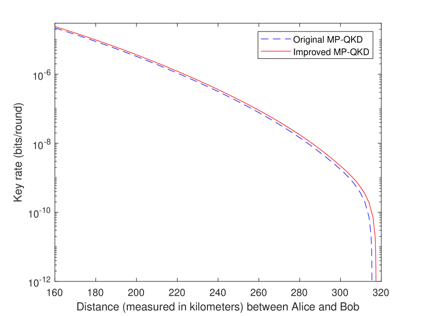
We use the same finite-key analysis and simulation model mentioned in ref.[33]. We set the total sending pulse as , the maximal pairing interval as , the misalignment error in Z basis as 0.5%, the misalignment error in X basis as 5%, the dark count rate as , the fiber loss coefficient as , the photon detection efficiency as 70%, the error correction inefficiency as and the failure probability when calculating the effect of statistical fluctuation as . Furthermore, we achieve a security level of in the sense of composable security against coherent attacks. The simulation results indicate a key rate improvement of over 10% for distances beyond , accompanied by an extended maximum achievable distance of , which once again confirms that our precise phase error analysis noticeably improves the key rate performance in practice.
IV CONCLUSION
In conclusion, our precise phase error rate analysis provides a comprehensive and accurate comprehension of phase error rate for QKD with phase postselection. The versatility of our method enables its direct integration into AOPP-SNS-TFQKD and MP-QKD protocols, facilitating notable enhancements in key rate performance without necessitating alterations to the existing experimental hardware or protocol steps. Given its adaptable nature, we anticipate its applicability to extend beyond these specific protocols, offering potential improvements in various other QKD with phase postselection.
*
Appendix A A more intuitive phase error analysis for SNS-TFQKD
In the equivalent entanglement-based scheme of SNS-TFQKD protocol, we can reformulate in (13) under the basis () as
| (22) |
Here we follow the idea proposed in [22] that the genuinely valid coded quantum state and the conjugated quantum state used for phase error estimation in SNS-TFQKD are similar to that in a BB84 protocol [1]. This indicates that the phase error rate defined in the basis is related to the yields of the quantum states and .
To estimate the phase error rate in the practical SNS-TFQKD protocol, Charlie should measure the bipartite signal qubits () sent from Alice and Bob on the measuring device . Since Charlie does not know the phase difference when measuring the signal qubits a and b, we can assume without loss of generality that Charlie’s measurement device can perfectly discriminate the quantum state between and , i.e., the click of the L port must indicate the quantum state and the click of the R port must indicate the quantum state . Naturally, Charlie can not perfectly discriminate whether the state is or ( or ), i.e., the click of the L port partially indicates the quantum state and the click of the R port partially indicates the quantum state . For the L port click events, we define the events caused by the quantum state as the error events, which enlightens us to define the quantum state as an error in the basis. Correspondingly, we define the events caused by the quantum state as the error events for the R port click events, which enlightens us to define the quantum state as an error in the basis.
We first consider the L port click events announced by Charlie. Alice and Bob prepare the joint quantum state in (13) and send the signal qubits a and b to Charlie for measuring. We define the phase error rate as
| (23) |
where, Re[z] is the real part of the complex number and is the quantum state of local auxiliary qubits A and B after Charlie’s measurement on signal states a and b.
In the decoy mode of SNS-TFQKD, Alice and Bob send the coherent states to Charlie for interference on the beamsplitter, followed by two photon detectors L and R. This allows us to estimate the yield of the quantum state which indicates the phase error rate for the L port click events.
| (24) |
where . In fact, is not the optimal phase error rate definition. We can use the current measurement data to estimate the precise phase error rate in the basis as follows
| (25) |
Combining (24) and (25), we have
| (26) |
Similarly, we define the phase error rate for the R port click events as
| (27) |
Alice and Bob also use the sent quantum state to estimate the phase error rate for the R port click events as follows
| (28) |
The precise phase error rate is
| (29) |
Combining (28) and (29), we also have
| (30) |
In the current SNS-TFQKD system, we usually consider the click events of the L and R ports together to calculate the total phase error rate
| (31) |
where and are the number of click events from port L and R. The loose phase error rate . The precise phase error rate . Combining (26) and (30), we can get the precise phase error rate from the loose phase error rate given the measurement data
| (32) |
Acknowledgements.
We acknowledge Dr. Rong Wang for the enlightening discussions. This work has been supported by the National Key Research and Development Program of China (Grant No. 2020YFA0309802), the National Natural Science Foundation of China (Grant Nos. 62171424, 62271463), Prospect and Key Core Technology Projects of Jiangsu provincial key R & D Program (BE2022071), the Fundamental Research Funds for the Central Universities, the Innovation Program for Quantum Science and Technology (Grant No. 2021ZD0300701).References
- Bennett and Brassard [1984] C. H. Bennett and G. Brassard, Quantum cryptography: Public key distribution and coin tossing, in Proceedings of IEEE International Conference on Computers, Systems and Signal Processing (IEEE, 1984) pp. 175–179.
- Ekert [1991] A. K. Ekert, Quantum cryptography based on bell’s theorem, Phys. Rev. Lett. 67, 661 (1991).
- Mayers [1996] D. Mayers, Quantum key distribution and string oblivious transfer in noisy channels, in Advances in Cryptology — CRYPTO ’96 (Springer Berlin Heidelberg, 1996) pp. 343–357.
- Lo and Chau [1999] H.-K. Lo and H. F. Chau, Unconditional security of quantum key distribution over arbitrarily long distances, Science 283, 2050 (1999).
- Shor and Preskill [2000] P. W. Shor and J. Preskill, Simple proof of security of the bb84 quantum key distribution protocol, Phys. Rev. Lett. 85, 441 (2000).
- Renner [2005] R. Renner, Security of Quantum Key Distribution, Ph.D. thesis, School Swiss Federal Institute of Technology Zurich (2005).
- Koashi [2009] M. Koashi, Simple security proof of quantum key distribution based on complementarity, New J. Phys. 11, 045018 (2009).
- König et al. [2007] R. König, R. Renner, A. Bariska, and U. Maurer, Small accessible quantum information does not imply security, Phys. Rev. Lett. 98, 140502 (2007).
- Tomamichel et al. [2012] M. Tomamichel, C. C. W. Lim, N. Gisin, and R. Renner, Tight finite-key analysis for quantum cryptography, Nat. Commun. 3, 634 (2012).
- Curty et al. [2014] M. Curty, F. Xu, W. Cui, C. C. W. Lim, K. Tamaki, and H.-K. Lo, Finite-key analysis for measurement-device-independent quantum key distribution, Nat. Commun. 5, 3732 (2014).
- Maeda et al. [2019] K. Maeda, T. Sasaki, and M. Koashi, Repeaterless quantum key distribution with efficient finite-key analysis overcoming the rate-distance limit, Nat. Commun. 10, 3140 (2019).
- Wang et al. [2021] R. Wang, Z.-Q. Yin, H. Liu, S. Wang, W. Chen, G.-C. Guo, and Z.-F. Han, Tight finite-key analysis for generalized high-dimensional quantum key distribution, Phys. Rev. Res. 3, 023019 (2021).
- Portmann and Renner [2022] C. Portmann and R. Renner, Security in quantum cryptography, Rev. Mod. Phys. 94, 025008 (2022).
- Hwang [2003] W.-Y. Hwang, Quantum key distribution with high loss: Toward global secure communication, Phys. Rev. Lett. 91, 057901 (2003).
- Wang [2005] X.-B. Wang, Beating the photon-number-splitting attack in practical quantum cryptography, Phys. Rev. Lett. 94, 230503 (2005).
- Lo et al. [2005] H.-K. Lo, X. Ma, and K. Chen, Decoy state quantum key distribution, Phys. Rev. Lett. 94, 230504 (2005).
- Lo et al. [2012] H.-K. Lo, M. Curty, and B. Qi, Measurement-device-independent quantum key distribution, Phys. Rev. Lett. 108, 130503 (2012).
- Braunstein and Pirandola [2012] S. L. Braunstein and S. Pirandola, Side-channel-free quantum key distribution, Phys. Rev. Lett. 108, 130502 (2012).
- Sasaki et al. [2014] T. Sasaki, Y. Yamamoto, and M. Koashi, Practical quantum key distribution protocol without monitoring signal disturbance, Nature 509, 475 (2014).
- Lucamarini et al. [2018] M. Lucamarini, Z. L. Yuan, J. F. Dynes, and A. J. Shields, Overcoming the rate–distance limit of quantum key distribution without quantum repeaters, Nature 557, 400 (2018).
- Ma et al. [2018] X. Ma, P. Zeng, and H. Zhou, Phase-matching quantum key distribution, Phys. Rev. X 8, 031043 (2018).
- Wang et al. [2018] X.-B. Wang, Z.-W. Yu, and X.-L. Hu, Twin-field quantum key distribution with large misalignment error, Phys. Rev. A 98, 062323 (2018).
- Lin and Lütkenhaus [2018] J. Lin and N. Lütkenhaus, Simple security analysis of phase-matching measurement-device-independent quantum key distribution, Phys. Rev. A 98, 042332 (2018).
- Cui et al. [2019] C. Cui, Z.-Q. Yin, R. Wang, W. Chen, S. Wang, G.-C. Guo, and Z.-F. Han, Twin-field quantum key distribution without phase postselection, Phys. Rev. Appl. 11, 034053 (2019).
- Curty et al. [2019] M. Curty, K. Azuma, and H.-K. Lo, Simple security proof of twin-field type quantum key distribution protocol, npj Quantum Inf. 5, 64 (2019).
- Wang et al. [2020] R. Wang, Z.-Q. Yin, F.-Y. Lu, S. Wang, W. Chen, C.-M. Zhang, W. Huang, B.-J. Xu, G.-C. Guo, and Z.-F. Han, Optimized protocol for twin-field quantum key distribution, Commun. Phys. 3, 149 (2020).
- Zhou et al. [2022] Y. Zhou, Z.-Q. Yin, R.-Q. Wang, S. Wang, W. Chen, G.-C. Guo, and Z.-F. Han, Twin-field quantum key distribution with partial phase postselection, Phys. Rev. Appl. 18, 054026 (2022).
- Xu et al. [2020] H. Xu, Z.-W. Yu, C. Jiang, X.-L. Hu, and X.-B. Wang, Sending-or-not-sending twin-field quantum key distribution: Breaking the direct transmission key rate, Phys. Rev. A 101, 042330 (2020).
- Jiang et al. [2021] C. Jiang, X.-L. Hu, Z.-W. Yu, and X.-B. Wang, Composable security for practical quantum key distribution with two way classical communication, New J. Phys. 23, 063038 (2021).
- Zhou et al. [2023] Y. Zhou, Z.-Q. Yin, S. Wang, W. Chen, G.-C. Guo, and Z.-F. Han, Twin-field quantum key distribution with three mutually unbiased bases, Phys. Rev. A 107, 032621 (2023).
- Zeng et al. [2022] P. Zeng, H. Zhou, W. Wu, and X. Ma, Mode-pairing quantum key distribution, Nat. Commun. 13, 3903 (2022).
- Xie et al. [2022] Y.-M. Xie, Y.-S. Lu, C.-X. Weng, X.-Y. Cao, Z.-Y. Jia, Y. Bao, Y. Wang, Y. Fu, H.-L. Yin, and Z.-B. Chen, Breaking the rate-loss bound of quantum key distribution with asynchronous two-photon interference, PRX Quantum 3, 020315 (2022).
- Wang et al. [2023] Z.-H. Wang, R. Wang, Z.-Q. Yin, S. Wang, F.-Y. Lu, W. Chen, D.-Y. He, G.-C. Guo, and Z.-F. Han, Tight finite-key analysis for mode-pairing quantum key distribution, Commun. Phys. 6, 265 (2023).
- Pirandola et al. [2017] S. Pirandola, R. Laurenza, C. Ottaviani, and L. Banchi, Fundamental limits of repeaterless quantum communications, Nat. Commun. 8, 15043 (2017).
- Takeoka et al. [2014] M. Takeoka, S. Guha, and M. M. Wilde, Fundamental rate-loss tradeoff for optical quantum key distribution, Nat. Commun. 5, 5235 (2014).
- Yu et al. [2019] Z.-W. Yu, X.-L. Hu, C. Jiang, H. Xu, and X.-B. Wang, Sending-or-not-sending twin-field quantum key distribution in practice, Sci. Rep. 9, 3080 (2019).
- Jiang et al. [2020] C. Jiang, X.-L. Hu, H. Xu, Z.-W. Yu, and X.-B. Wang, Zigzag approach to higher key rate of sending-or-not-sending twin field quantum key distribution with finite-key effects, New J. Phys. 22, 053048 (2020).