The Inertial Spin Model of flocking with position-dependent forces

Abstract

We consider the inertial spin model (ISM) of flocking and swarming. The model has been introduced to explain certain dynamic features of swarming (second sound, a lower than expected dynamic critical exponent) while preserving the mechanism for onset of order provided by the Vicsek model. The ISM has only been formulated with an imitation (“ferromagnetic”) interaction between velocities. Here we show how to add position-dependent forces in the model, which allows to consider effects such as cohesion, excluded volume, confinement and perturbation with external position-dependent field. We study numerically a one-particle case.

I Introduction

Collective animal motion Sumpter (2006); Vicsek and Zafeiris (2012) is a particularly striking aspect of emergent collective behavior where collective order (as in flocks of birds flying together) can arise from simple short-range interactions between individuals. Several models have been proposed to describe flocking behavior, dating back at least to the 1980s Aoki (1982); Reynolds (1987). The paradigmatic Vicsek model of flocking Vicsek et al. (1995); Ginelli (2016) (and the related Toner-Tu field theory Toner and Tu (1995, 1998); Toner (2012)) has received much attention from the statistical physics community because it predicts the appearance of ordered flocks starting with a simple set of microscopic local rules, similar to the way ferromagnetic order arises in the Ising or Heisenberg models. It turns out that the phase diagram of the Vicsek model is more complicated than that of the classic ferromagnetic order-disorder transition, featuring a discontinuous transition and region with microphase separation (see Chaté (2020) for a review); however it remains true that it allows to explain how a flock with fully ordered velocities can result from a local “ferromagnetic” imitation rule.

Although the Vicsek model is successful in explaining the thermodynamics of flocking, it is not suitable to interpret certain dynamical features related to the presence of inertial effects. The finding of wave-like propagation of direction information during turns in starling flocks Attanasi et al. (2014a) led to the proposal of the inertial spin model (ISM) Cavagna et al. (2014), which we consider here. The model is described in detail in Sec. II.1, but it is essentially the Vicsek model endowed with a Hamiltonian-like (second order) dynamics, so that second time derivative of the velocity is proportional to the effective social force, instead of the first time derivative as in Vicsek. Although it is true that in the thermodynamic limit the large-scale behavior is described by an over-damped theory Cavagna et al. (2019a), namely the Toner-Tu Toner and Tu (1998) hydrodynamic theory (which is a coarse-grained version of the Vicsek model), inertial effects can be observed in finite systems Cavagna et al. (2015). This is relevant in the description of observations of biological flocks, which at sizes of a few thousands of individuals are large but still far enough from the thermodynamic limit that finite-size effects are important. In the language of the renormalization group (RG), a crossover phenomenon arises in the RG flow such that at intermediate sizes the global properties will be described by an inertial fixed point with an unstable direction, instead of the stable over-damped fixed point that rules in the thermodynamic limit Cavagna et al. (2019b).

The dynamic critical behavior of midge swarms Cavagna et al. (2017) also displays inertial effects. At moderate system size, the Vicsek transition looks continuous Chaté et al. (2008a), and it can be used to interpret static aspects of swarms such as the presence of scale-free correlations Attanasi et al. (2014b), but it is again insufficient to account for the dynamic behavior. In particular the dynamic critical exponent of the Toner-Tu theory Chen et al. (2015) is higher than the experimental value. A coarse-grained version of the ISM was recently employed Cavagna et al. (2023a) to show that both inertia and activity are needed to explain the observations.

The ISM was introduced in refs. Attanasi et al. (2014a); Cavagna et al. (2014) (see also the review Cavagna et al. (2018)). The formation of flocks at $T=0$ was considered in Ha et al. (2019) and Markou (2021), while the finite-temperature equilibrium in the mean-field case was studied in Benedetto et al. (2020) and Ko et al. (2023), and Huh and Kim (2022) considered a variant incorporating uniform external fields controlling alignment and rotation, but with a sort of mean-field spin. In these works, as well as in the numerical simulations of Cavagna et al. (2014, 2023a), infinite space or periodic boundary conditions were employed.

In this work we consider extending the ISM to include position-dependent forces. In the original ISM the interaction is between velocities (actually, velocity directions), such that particles tend to align the velocities with each other, just as in the Vicsek model. Positions enter the picture only indirectly, through the definition of the interaction network (which can be metric or topological Kumar and De (2021)). There are several reasons why positional forces are desirable. To treat finite systems with metric interactions it is necessary to introduce some kind of confinement, because otherwise small velocity fluctuations eventually lead to particles becoming isolated from the flock and thus “evaporating” the system to infinite dilution. This can be avoided using reflecting boundary conditions, external fields, or inter-particle interactions providing cohesion. Reflecting walls for confinement Chepizhko et al. (2021) or partial confinement Tu et al. (1998); Morin and Bartolo (2018); Moreno et al. (2020), and cohesion through attractive forces Chaté et al. (2008b) have been considered for the Vicsek case. Position-dependent inter-particle interactions may also be included for other purposes, e.g. to add an excluded volume potential that will limit the local density Tu et al. (1998). A position-dependent external field can also be interesting to study perturbation and response: a field coupled to the velocities is straightforward to add (as it has been done for Vicsek Kyriakopoulos et al. (2016)), but experimentally it may be easier to impose a perturbation with a position-dependent field, for example by implementing a moving artificial marker to perturb an insect swarm Attanasi et al. (2014c).

Given the Hamiltonian structure of the ISM, which involves velocity and spin as canonical variables, it is not immediately obvious what is the best way to add a position-dependent force. We discuss this in the next section. After proposing a consistent way to implement these forces, we explore numerically some results regarding field-induced confinement.

II Inertial Spin model with external position-dependent forces

Originally, the ISM was proposed Attanasi et al. (2014a); Cavagna et al. (2014) based on the experimental observation of second sound (i.e. order-parameter waves) in the turning of starling flocks Attanasi et al. (2014a). Second sound is an indication that an inertial mechanism is at work that results in propagation with constant speed (vs. diffusive propagation as it occurs in the overdamped case). The goal is then to formulate a model with the static properties of Vicsek’s model (i.e. capable of spontaneously producing orientational order) but with inertial rather than diffusive dynamics Cavagna et al. (2018). It seems thus reasonable to seek a Hamiltonian formulation, as this will lead naturally to canonical (i.e. inertial) equations of motion. One then needs to identify the correct canonical coordinate / conjugate momentum pair. A key observation is that when a flock changes direction of motion individual birds turn following paths of approximately the same radius, rather than following parallel paths. This suggests that invariance under internal (rather than global) rotations is the relevant symmetry. Indeed, equal-radius turns are not generated by rigid rotations (as are parallel-path turns), but by rotations of the internal orientation of each individual, which moves at approximately constant speed. These considerations lead to recognize the Vicsek interaction as an interaction between orientations, rather than velocities, and to propose a Hamiltonian formalism in which the particle orientation is the canonical coordinate. Its canonical conjugate, the spin, is the generator of internal rotations.

In a Hamiltonian theory, the symmetry under internal rotations leads to conservation of the spin (the corresponding momentum). Indeed this quantity can be conserved in an equal-radius turn, in contrast to the angular momentum (generator of global, rigid rotations). Angular momentum could be conserved in a turn following parallel paths, but this is forbidden by the requirement of constant speed. However, spin conservation cannot be expected to hold exactly, so dissipation of the spin is introduced by adding noise and friction terms (as in the standard Langevin equation) in the spin equation of motion. This is how temperature enters the theory, making it possible to tune the system between order and disorder.

II.1 The original ISM

Let us first introduce the original ISM and then our proposal to include position-dependent forces. For what follows, it is convenient to derive the ISM using the velocity of the $i$-th particle $\mathbf{v}_{i}$ and its canonical conjugate, instead of orientation and spin. We do not consider speed fluctuations, so that a set of hard constraints

$$f_{i}(\mathbf{v}_{i})=\mathbf{v}_{i}^{2}-v_{0}^{2}=0$$ (1)

will be imposed. Note however that $\mathbf{v}_{i}$ is treated as an internal canonical coordinate, and completely unrelated, as far as the Hamiltonian formalism is concerned, to the usual mechanical momentum. Its canonical momentum, which we call $\mathbf{w}_{i}$, is defined by

$$\{v_{i}^{\mu},w_{j}^{\nu}\}=\delta_{ij}\delta^{\mu\nu},$$ (2)

where $\{\ldots\}$ are Poisson brackets. The Hamiltonian formalism applies to the space of the internal degrees of freedom $(\mathbf{v}_{i},\mathbf{w}_{i})$; the connection between $\mathbf{v}_{i}$ and the actual particle velocity is made through an extra equation

$$\dot{\mathbf{r}_{i}}=\mathbf{v}_{i},$$ (3)

which complements the canonical equations of motion. Since $\mathbf{r}_{i}$ is also a parameter of the Hamiltonian (via the potential), the whole theory is in this sense pseudo-Hamiltonian.

One proposes a Hamiltonian

$$\mathcal{H}=\sum_{i}\frac{w_{i}^{2}}{2\mu}+\mathcal{V}(\{\mathbf{v}_{i}\})+\sum_{i}\lambda_{i}f_{i}(\mathbf{v}_{i}).$$ (4)

The first term, which has the form of a kinetic energy, introduces inertia, with $\mu$ a social, or effective, mass. The role of the third term is to enforce the constraints through the Lagrange multipliers $\lambda_{i}$. The second term is an interaction potential, which in the ISM is chosen to implement Vicsek’s Vicsek et al. (1995) velocity-imitation. In continuous time this is obtained from

$$\mathcal{V}(\{\mathbf{v}_{i}\})=\frac{J}{v_{0}^{2}}\sum_{ij}n_{ij}\mathbf{v}_{i}\cdot\mathbf{v}_{j},$$ (5)

with $J$ a coupling constant and $n_{ij}$ the adjacency matrix, which defines the interaction network ($n_{ij}=1$ if $i$ and $j$ are interacting neighbours, and 0 if not). Positions enter into $\mathcal{H}$ through the adjacency matrix, which can be defined to implement metric (through a cut-off radius) or topological (by choosing a fixed number of nearest neighbors) interactions. As far as the Hamiltonian formalism is concerned, positions are just parameters of the potential, but the extra equation $\dot{\mathbf{r}}_{i}=\mathbf{v}_{i}$ turns them into coordinates, and the model into an active model.

The canonical equations of motion are

$$\dot{\mathbf{v}}_{i} =\frac{\partial\mathcal{H}}{\partial\mathbf{w}_{i}}=\frac{\mathbf{w}_{i}}{\mu},$$ (6a)

$$\dot{\mathbf{w}}_{i} =-\frac{\partial\mathcal{H}}{\partial\mathbf{v}_{i}}=\mathbf{f}_{i}-2\lambda_{i}\mathbf{v}_{i},$$ (6b)

where $\mathbf{f}_{i}=\partial\mathcal{V}/\partial\mathbf{v}_{i}$ is the interaction force. The Lagrange multipliers can be found using the relations $\dot{\mathbf{v}}_{i}\cdot\mathbf{v}_{i}=0$ and $\left(\dot{\mathbf{v}}_{i}\right)^{2}+\mathbf{v}_{i}\cdot\ddot{\mathbf{v}}_{i}=0$, which follow from the first and second time derivatives of the constraint. Eq. (6b) is then

$$\dot{\mathbf{w}}_{i}=\mathbf{f}_{i}^{\perp}-\frac{\left(\dot{\mathbf{v}}_{i}\right)^{2}}{v_{0}^{2}}\mathbf{v}_{i},$$ (7)

with $\perp$ denoting the projection in the direction perpendicular to the velocity:

$$\mathbf{a}^{\perp}=\mathbf{a}-(\mathbf{a}\cdot\mathbf{v}_{i})\frac{\mathbf{v}_{i}}{v_{0}^{2}}=-\frac{1}{v_{0}^{2}}\mathbf{v}_{i}\times\left(\mathbf{v}_{i}\times\mathbf{a}\right).$$ (8)

Now it is convenient to introduce the spin of the $i$-th particle as $\mathbf{s}_{i}=\mathbf{v}_{i}\times\mathbf{w}_{i}$. The Poisson brackets

$$\{s_{i}^{\mu},v_{j}^{\nu}\}=\delta_{ij}\epsilon^{\mu\nu\rho}v^{\rho},\qquad\{s_{i}^{\mu},w_{j}^{\nu}\}=\delta_{ij}\epsilon^{\mu\nu\rho}w^{\rho},$$ (9)

where greek superindices indicate cartesian components, $\delta_{ij}$ is Kroneker’s delta and $\epsilon^{\mu\nu\rho}$ is the completely antisymmetric tensor, show that $\mathbf{s}_{i}$ does generate the internal rotations. Using the constraint again, the condition $\mathbf{v}_{i}\cdot\mathbf{w}_{i}=0$ allows to express the momentum in terms of the spin, $\mathbf{w}_{i}=-\mathbf{v}_{i}\times\mathbf{s}_{i}/v_{0}^{2}$ and the Hamiltonian can be written as

$$\mathcal{H}=\sum_{i}\frac{\mathbf{s}_{i}^{2}}{2\chi}+\mathcal{V}(\{\mathbf{v}_{i}\}),$$ (10)

defining $\chi=v_{0}^{2}\mu$. The final equations of the ISM are

$$\dot{\mathbf{r}}_{i} =\mathbf{v}_{i},$$ (11a)

$$\dot{\mathbf{v}}_{i} =\frac{1}{\chi}\mathbf{s}_{i}\times\mathbf{v}_{i},$$ (11b)

$$\dot{\mathbf{s}}_{i} =\mathbf{v}_{i}\times\left[\frac{J}{v_{0}^{2}}\sum_{j}n_{ij}\mathbf{v}_{j}-\frac{\eta}{v_{0}^{2}}\dot{\mathbf{v}}_{i}+\frac{1}{v_{0}}\bm{\xi}_{i}\right],$$ (11c)

where we have added the friciton and stochastic terms, with $\langle\xi_{i}^{\mu}(t)\rangle=0$, $\langle\xi_{i}^{\mu}(t)\xi_{j}^{\nu}(t^{\prime})\rangle=2\eta T\delta_{ij}\delta^{\mu\nu}\delta(t-t^{\prime})$. Note that (11b) and the deterministic part of (11c) can be derived either substituting $\mathbf{s}_{i}$ for $\mathbf{w}_{i}$ in (6) or directly from the Hamiltonian (10) and the Poisson brackets

$$\dot{\mathbf{v}}_{i} =\left\{\mathbf{v}_{i},\mathcal{H}\right\}=-\mathbf{v}_{i}\times\frac{\partial\mathcal{H}}{\partial\mathbf{s}_{i}},$$ (12a)

$$\dot{\mathbf{s}}_{i} =\left\{\mathbf{s}_{i},\mathcal{H}\right\}=-\mathbf{v}_{i}\times\frac{\partial\mathcal{H}}{\partial\mathbf{v}_{i}}-\mathbf{s}_{i}\times\frac{\partial\mathcal{H}}{\partial\mathbf{s}_{i}}.$$ (12b)

In contrast, (11a) does not follow from $\{\mathbf{r},\mathcal{H}\}$.

II.2 Position-dependent forces

Now we want to introduce position-dependent forces and fields. While a velocity-dependent field can be added quite naturally in the formalism as a new term $H_{\textrm{field}}(\mathbf{v}_{i})$ in Hamiltonian (10), position-dependent forces require some thought because position is not part of the canonical variables of this Hamiltonian. There are in principle two ways to add these forces. One can expect that they should appear in (11b), or (6a), just as in ordinary Newton’s equation. Alternatively, one can argue that the forces should appear in (11c) or (6b), since it is this equation that encodes the inertial mechanism that controls motion in this model. We shall add both kind of force, but it will turn out that both can be handled as a new force in the spin equation, provided it depends on the velocity in a specific way.

The forces must be added in a way that respects the constraint of constant speed, so that it is convenient to start with (4), which uses $\mathbf{w}_{i}$ and includes the constraint explicitly through the multipliers $\lambda_{i}$. We propose to add the forces writing

$$\begin{split}\mathcal{H}=&{}\sum_{i}\frac{w^{2}}{2\mu}+\mathcal{V}(\{\mathbf{v}_{i}\})-\sum_{i}\mathbf{v}_{i}\cdot\mathbf{F}(\{\mathbf{r}\})\\ &+\sum_{i}\mathbf{w}\cdot\frac{\mathbf{G}(\{\mathbf{r}\})}{m}+\sum_{i}\lambda_{i}(v_{i}^{2}-v_{0}^{2}),\end{split}$$ (13)

where $\mathbf{G}$ and $\mathbf{F}$ are the new position-dependent forces and we have allowed the possibility that the mass associated to the positional force, $m$, is different from $\mu$. The corresponding canonical equations are

$$\dot{\mathbf{v}}_{i} =\frac{\partial\mathcal{H}}{\partial\mathbf{w}_{i}}=\frac{\mathbf{w}_{i}}{\mu}+\frac{\mathbf{G}_{i}}{m},$$ (14a)

$$\dot{\mathbf{w}}_{i} =-\frac{\partial\mathcal{H}}{\partial\mathbf{v}_{i}}=-\frac{\partial\mathcal{V}}{\partial\mathbf{v}_{i}}+\mathbf{F}_{i}-2\lambda_{i}\mathbf{v}_{i},$$ (14b)

where again to eliminate the $\lambda_{i}$ one uses the fact that first and second time derivatives of the constraints must vanish together with the equations of motion to find

$$\lambda_{i}=\frac{\mu}{2v_{0}^{2}}\left(\frac{\mathbf{w}_{i}}{\mu}+\frac{\mathbf{G}_{i}}{m}\right)^{2}+\frac{\mathbf{v}_{i}}{2v_{0}^{2}}\cdot\left(\mathbf{f}_{i}+\mathbf{F}_{i}\right)+\frac{\mu}{2mv_{0}^{2}}\dot{\mathbf{G}}_{i}\cdot\mathbf{v}_{i}.$$ (15)

Eq. (14b) becomes then

$$\dot{\mathbf{w}}_{i}=\mathbf{f}_{i}^{\perp}+\mathbf{F}_{i}^{\perp}-\frac{\mu}{v_{0}^{2}}\left(\frac{\mathbf{w}_{i}}{\mu}+\frac{\mathbf{G}_{i}}{m}\right)^{2}\mathbf{v}_{i}-\frac{\mu}{mv_{0}^{2}}(\dot{\mathbf{G}}_{i}\cdot\mathbf{v}_{i})\mathbf{v}_{i}.$$ (16)

As before, the equations assume a simpler form if one introduces the spin. Defining $\mathbf{s}_{i}=\mathbf{v}_{i}\times\mathbf{w}_{i}$, this can be inverted with the help of the constraint to find $\mathbf{w}_{i}=-\mu(\mathbf{v}_{i}\cdot\mathbf{G}_{i})/(mv_{0}^{2})-\mathbf{v}_{i}\times\mathbf{s}_{i}/v_{0}^{2}$ and rewrite (14a) and (16) as

$$\dot{\mathbf{v}}_{i} =-\frac{1}{\chi}\mathbf{v}_{i}\times\left[\mathbf{s}_{i}+\frac{\mu}{m}\mathbf{v}_{i}\times\mathbf{G}_{i}\right],$$ (17a)

$$\dot{\mathbf{s}}_{i} =\mathbf{v}_{i}\times\left(\mathbf{f}_{i}+\mathbf{F}_{i}\right)-\frac{\chi}{X^{2}}(\mathbf{v}_{i}\cdot\mathbf{G}_{i})(\mathbf{G}_{i}\times\mathbf{v}_{i})$$

$$\quad-\frac{1}{X}\mathbf{G}_{i}\times(\mathbf{v}_{i}\times\mathbf{s}_{i}),$$ (17b)

with $\chi=v_{0}^{2}\mu$, $X=v_{0}^{2}m$, which reduce to (11) (apart from noise) when $\mathbf{F}_{i}=\mathbf{G}_{i}=0$. Eqs. (17) can be further simplified, because not every form of $\mathbf{G}_{i}$ will lead to observable changes in particle trajectories. The situation is similar to the case of the Hamiltonian formulation of electromagnetic forces, where a gauge transformation alters the vector potential but not the trajectories. This can be seen by redefining the momentum and spin. Eqs. (14a) and (17a) suggest to define $\mathbf{z}_{i}=\mathbf{w}_{i}+(\mu/m)\mathbf{G}_{i}$, and $\tilde{\mathbf{s}}_{i}=\mathbf{v}_{i}\times\mathbf{z}_{i}$. Renaming $\tilde{\mathbf{s}}_{i}\longrightarrow\mathbf{s}_{i}$ and adding the stochastic terms the equations of motion finally read

$$\dot{\mathbf{v}}_{i} =\frac{1}{\chi}\mathbf{s}_{i}\times\mathbf{v}_{i},$$ (18a)

$$\dot{\mathbf{s}}_{i} =\mathbf{v}_{i}\times\left[-\frac{\partial\mathcal{V}}{\partial\mathbf{v}_{i}}+\mathbf{F}_{i}+\frac{\chi}{X}(\mathbf{v}_{i}\cdot\nabla)\mathbf{G}_{i}\right]+$$

$$\mathbf{v}_{i}\times\left[-\frac{\eta}{v_{0}^{2}}\dot{\mathbf{v}}_{i}+\frac{1}{v_{0}}\bm{\xi}_{i}\right].$$ (18b)

The final equations of motion cannot be written from Poisson brackets, because $\mathbf{r}_{i}$ is not a canonical coordinate, and in consequence $\dot{\mathbf{G}}_{i}=(\mathbf{v}_{i}\cdot\nabla)\mathbf{G}_{i}$ does not follow naturally from $\{\mathbf{G},\mathcal{H}\}$. However it is possible to write a slightly different Hamiltonian that will yield (18) from $\dot{\mathbf{v}}_{i}=\{\mathbf{v}_{i},\mathcal{H}\}$, $\dot{\mathbf{s}}_{i}=\{\mathbf{s}_{i},\mathcal{H}\}$, provided $\mathbf{G}_{i}$ can be written as a gradient, $\mathbf{G}_{i}=\nabla\Gamma_{i}$:

$$\begin{split}\mathcal{H}={}&\sum_{i}\frac{s_{i}^{2}}{2\chi}+\mathcal{V}(\{\mathbf{v}_{i}\})-\sum_{i}\mathbf{v}_{i}\cdot\mathbf{F}_{i}(\mathbf{r}_{i})+\\ &\frac{\mu}{2m}\sum_{i\mu\nu}v_{i}^{\mu}v_{i}^{\nu}\frac{\partial^{2}\Gamma(\mathbf{r}_{i})}{\partial r_{i}^{\mu}\partial r_{i}^{\mu}}.\end{split}$$ (19)

II.3 Overdamped limit and dimensionless quantities

It is possible to eliminate $\mathbf{s}_{i}$ and write a single, second-order, equation of motion for the velocity. This can be more convenient for numerical integration, as then one can apply one of the well-known discretizations used in molecular or stochastic dynamics (see e.g. Cavagna et al., 2016)

$$\chi\frac{\ddot{\mathbf{v}}_{i}}{v_{0}}+\chi\frac{(\dot{\mathbf{v}}_{i})^{2}}{v_{0}^{2}}\frac{\mathbf{v}_{i}}{v_{0}}+\eta\frac{\dot{\mathbf{v}}_{i}}{v_{0}}=\\ J\sum_{j}n_{ij}\frac{\mathbf{v}_{j}^{\perp}}{v_{0}}+v_{0}\mathbf{F}^{\perp}+\frac{\chi}{X}\left(\frac{\mathbf{v}_{i}}{v_{0}}\cdot\nabla\right)v_{0}^{2}\mathbf{G}_{i}^{\perp}+\bm{\xi}$$ (20)

Writing the equation in this way makes it clear that the lhs is independent of $v_{0}$ (in effect, we are writing an equation of motion for the orientation), and so must the rhs. The interaction force is clearly independent of $v_{0}$ (as it should since it comes from a potential energy involving orientations), but in this form we realize that the positional forces must be such that $v_{0}\mathbf{F}_{i}$ and $v_{0}^{2}\mathbf{G}_{i}$ are independent of the speed. For what follows it’s then convenient to introduce $\bm{\psi}_{i}=\mathbf{v}_{i}/v_{0}$.

We now seek the overdamped limit of (20). Rescaling the time $t\to\hat{t}=t/a$ we have $\hat{\mathbf{x}}_{i}(\hat{t})=\hat{\mathbf{x}}_{i}(t/a)=\mathbf{x}_{i}(t)$, $\hat{\mathbf{v}}_{i}(\hat{t})=d\hat{\mathbf{x}}/d\hat{t}=a\mathbf{v}$, $\hat{v}_{0}=av_{0}$, $\hat{\bm{\psi}}(\hat{t})=\hat{\mathbf{v}}/\hat{v}_{0}=\bm{\psi}(t)$, and $\dot{\hat{\psi}}=a\dot{\psi}$, so that

$$\frac{\chi}{a^{2}}\ddot{\hat{\bm{\psi}}}_{i}+\frac{\chi}{a^{2}}(\dot{\hat{\bm{\psi}}}_{i})^{2}\hat{\bm{\psi}}_{i}+\frac{\eta}{a}\dot{\hat{\bm{\psi}}}_{i}=\\ J\sum_{j}n_{ij}\hat{\bm{\psi}}_{j}^{\perp}+v_{0}\mathbf{F}^{\perp}+\frac{\chi}{X}\left(\hat{\bm{\psi}}_{i}\cdot\nabla\right)v_{0}^{2}\mathbf{G}_{i}^{\perp}+\sqrt{\frac{2T\eta}{a}}f(\hat{t}),$$ (21)

where $\langle f(\hat{t})f({\hat{t}}^{\prime})\rangle=\delta(\hat{t}-\hat{t}^{\prime})$. Choosing $a\propto\eta$ one arrives at an equation that will become first order in the limit $\chi/\eta^{2}\to 0$. It is convenient that $a$ have units of time so that $\hat{t}$ is non-dimensional. We choose $a=\eta/J$ , and write the equations of motion as

$$\dot{\hat{\mathbf{x}}} =\hat{v}_{0}\hat{\bm{\psi}}(\hat{t})$$ (22a)

$$\Omega\ddot{\hat{\bm{\psi}}}_{i}+\Omega(\dot{\hat{\bm{\psi}}}_{i})^{2}\hat{\bm{\psi}}_{i}+\dot{\hat{\bm{\psi}}}_{i} =\sum_{j}n_{ij}\hat{\bm{\psi}}_{j}^{\perp}+\hat{\mathbf{F}}^{\perp}$$

$$\quad+\frac{\chi}{X}\left(\hat{\bm{\psi}}_{i}\cdot\nabla\right)\hat{\mathbf{G}}_{i}^{\perp}$$

$$\quad+\sqrt{\frac{2T}{J}}f(\hat{t}),$$ (22b)

where we have defined

$$\Omega =\frac{J\chi}{\eta^{2}},$$ (23a)

$$\hat{\mathbf{F}}_{i} =\frac{v_{0}}{J}\mathbf{F}_{i},$$ (23b)

$$\hat{\mathbf{G}}_{i} =\frac{v_{0}^{2}}{J}\mathbf{G}_{i}.$$ (23c)

All these quantities are dimensionless (provided one chooses the units of $\mathbf{G}$ so that $\mu$ and $m$ have the same units so that $\chi/X$ is non-dimensional, see Eq. (14a)).

$\Omega$ is a measure of the relative weight of inertia vs. dissipation. The overdamped limit is obtained taking $\Omega\to 0$, in which case the equation for the orientation becomes first-order, yielding a continuous-time version of the Vicsek model:

$$\dot{\hat{\mathbf{x}}} =\hat{v}_{0}\hat{\bm{\psi}}(\hat{t})$$ (24a)

$$\dot{\hat{\bm{\psi}}}_{i} =\sum_{j}n_{ij}\hat{\bm{\psi}}_{j}^{\perp}+\hat{\mathbf{F}}^{\perp}+\frac{\chi}{X}\left(\hat{\bm{\psi}}_{i}\cdot\nabla\right)\hat{\mathbf{G}}_{i}^{\perp}$$

$$\quad+\sqrt{\frac{2T}{J}}f(\hat{t}).$$ (24b)

In what follows we shall consider the case of a single particle and a harmonic restoring force $\hat{\mathbf{F}}=-k\hat{\mathbf{x}}$. For this force, the overdamped equation (but not the full ISM) reduces to a form that looks like the harmonic oscillator,

$$\ddot{\hat{\mathbf{x}}}=-\hat{v}_{0}k\hat{\mathbf{x}}^{\perp}+v_{0}\sqrt{\frac{2T}{J}}f(\hat{t}),$$ (25)

but with a non-linearity introduced by the projector operator. Explicitly, going back to dimensionful time,

$$\eta\ddot{\mathbf{x}}=-kJv_{0}\mathbf{x}+kJv_{0}(\bm{\psi}\cdot\mathbf{x})\bm{\psi}+\sqrt{2\eta T}f(t).$$ (26)

III Numerical results

To gain some insight into the behavior of the modified model, we consider the case of a single particle in an external field to study the confinement effects. We solve the equations of motion numerically in their second-order form (20). We have employed an integration scheme used in Brownian Dynamics simulations Rapaport (2004), based on a Velocity Verlet integrator with Lagrange multipliers to enforce fixed speed. The procedure is described in detail in ref. Cavagna et al. (2016). We consider the simplest form of the force to achieve confinement, namely a simple harmonic force

$$\mathbf{F}_{i}=-\frac{1}{v_{0}}k_{0}\mathbf{x}_{i},$$ (27)

and set $\mathbf{G}_{i}=0$. All results shown are in 2-$d$.

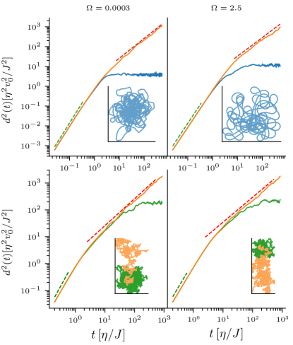
Figure 1: Mean squared displacement $d^{2}(t)$ vs. time for the ISM with harmonic confining force at different values of $\Omega$ and $k_{0}$. Left panels correspond to $\Omega=3\cdot 10^{-5}$, and right panels to $\Omega=2.5$. The top panels show the MSD for $k_{0}=1$ (blue) compared to the free particle ($k_{0}=0$, orange), and the lower panels have $k_{0}=0.02$ (green) and $k_{0}=0$. Note that the orange curves correspond to free particles with different inertia, hence the diffusive regime is reached at different times. The dashed lines have slope 2 (green) and 1 (orange) and are a guide to identify the ballistic and diffusive regimes. Time is measured in units of $\eta/J$ and position in units of $v_{0}\eta/J$. The MSD is an average over 100 trajectories. Insets show sample trajectories, with the same color code as the main panels.

The mean squared displacement (MSD) $d^{2}(t)=[\mathbf{x}(t)-\mathbf{x}(0)]^{2}$ is shown in Fig. 1 for the ISM with two different values of the dimensionless parameter $\Omega$ (23a) (recall $\Omega\gg 1$ means inertia dominates, while $\Omega\ll 1$ corresponds to overdamped systems) and different field strengths (i.e. different $k_{0}$). In all cases, for very short times there is a ballistic regime ($d^{2}\sim t^{2}$) which crosses over to a diffusive ($d^{2}\sim t$) regime for the free case. If the confining field is present, the displacement eventually saturates at an $\Omega$-dependent plateau (Fig. 2). For weak enough fields, the diffusive regime can be observed before the plateau, but at high fields the confinement effects manifest before the transition from ballistic to diffusive motion.

Figure 2: Maximum (plateau) of the mean squared displacement vs. $\Omega$ for the ISM with harmonic confinement, $k_{0}=1$.

The effects of confinement can also be noticeable in the velocity correlation function $C_{v}(t)=\langle\mathbf{v}(t)\cdot\mathbf{v}(0)\rangle$ (Fig. 3). If the confining field strength is large enough, there is a range of times for which anticorrelation is observed and followed, at high $\Omega$, by damped oscillations. The first anti-correlation minimum should not be mistaken for an inertial effect: it is due to the fact that the velocity changes direction due to the confinement force, and it is actually observed both at low and high $\Omega$ for large enough $k_{0}$. For $k_{0}=1$ it can be seen that $C_{v}(t)$ has its first minimum around $t\approx 3$, which is the time at which confinement effects start to be noticeable in $d^{2}(t)$ (cf. top panels of Fig. 1). At this time, the diffusive regime has not yet been reached, and correlation function of the free particle is still non-vanishing. In contrast, for weaker fields (e.g. $k_{0}=0.02$ in Fig. 3) it can happen that the MSD starts deviating towards the plateau already in the diffusive regime, when the velocity has lost correlation (as measured by $C_{v}(t)$ for the free case). In this case no anticorrelation minimum is observed. Inertial effects manifest, for large $k_{0}$, in the presence of damped oscillations in $C_{v}(t)$, lasting roughly during the transition from the ballistic regime to the plateau in the MSD. For all $k_{0}$, when $\Omega$ is large the correlation function has a flat derivative as $t\to 0$, a sign of second-order dynamics (see discussion in Cavagna et al. (2017)). This can be seen plotting $h(x)=-\log C(x)/x$ with $x=t/\tau$ and $\tau$ is the correlation time (Fig. 4). $h(x)$ tends to a constant for $x\to 0$ if $C(t)$ resembles a simple exponential for short times (overdamped system), or to 0 if $C(t)$ has a flat derivative. We have computed $\tau$ using the spectral definition Halperin and Hohenberg (1969),

$$\int_{0}^{\infty}\!\!\frac{dt}{t}\,\frac{C(t)}{C(t=0)}\sin\left(\frac{t}{\tau}\right)=\frac{\pi}{4}.$$ (28)

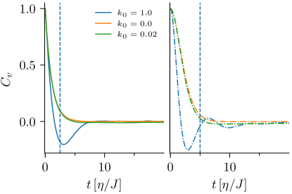
Figure 3: Velocity time correlation function $C_{v}(t)$ for $\Omega=3\cdot 10^{-4}$ (left) and $\Omega=2.5$ (right) and three values of $k_{0}$. The vertical dotted line indicates the time at which the system with $k_{0}=1$ starts feeling the confinement effects of the field (Fig. 1). For the lower value of $k_{0}$, confinement is only observed around $t\approx 20$ to 25$\,\eta/J$, which is out of the scale of the abscissa.

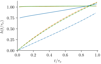
Figure 4: The function $h(x)=-\log C_{v}(x)/x|_{x=t/\tau}$ for $\Omega=3\cdot 10^{-4}$ (full lines) and $\Omega=2.5$ (dotted lines). Colors indicate values of $k_{0}$ as in Fig. 3.

The velocity time correlations look similar to those of an harmonic oscillator with Langevin dynamics, a system that might be considered a minimal model for a single confined particle. However, the behavior of the active system is different from the harmonic oscillator’s. One way to see this is considering the correlation times of the three dynamical variables position $\mathbf{x}$, velocity $\mathbf{v}$ and spin $\mathbf{s}$. Since the spin can be computed from the trajectories as $\mathbf{s}=\mu\mathbf{v}\times\dot{\mathbf{v}}$, this definition can also be applied to trajectories of the harmonic oscillator to obtain a correlation function $C_{s}(t)$, so we can compute the time correlation functions for position $C_{x}(t)$, velocity $C_{v}(t)$ and spin $C_{s}(t)$ in both systems. Writing the oscillator equation as

$$m\ddot{\mathbf{x}}+\eta\dot{\mathbf{x}}+k\mathbf{x}=\xi(t)$$ (29)

the inertial parameter is $\Omega_{\text{HO}}=km/\eta^{2}$. The ratios $\tau_{v}/\tau_{x}$ and $\tau_{s}/\tau_{x}$ show quite different behavior as a function of $\Omega$ or $\Omega_{\text{HO}}$ (Fig. 5). In the HO, both ratios increase monotonically as the system becomes more underdamped, while in the ISM $\tau_{v}/\tau_{x}$ is monotonically decreasing and $\tau_{s}/\tau_{x}$ reaches a maximum near $\Omega=1$ and then decreases. The third ratio, $\tau_{s}/\tau_{v}$, is monotonically increasing in both cases, but as $\Omega\to 0$ it tends to 1 for the HO while it goes to zero for the ISM, as in the latter the spin correlation time vanishes more quickly than that of the velocity.

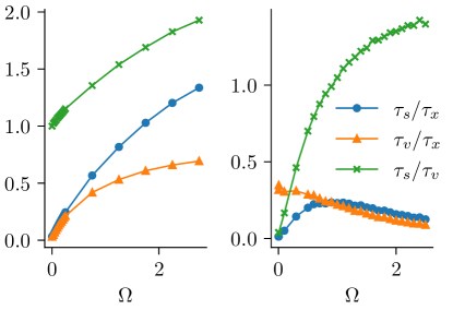
Figure 5: Correlation times ratios vs. inertial parameter for the 2-$d$ stochastic harmonic oscillator (left) and ISM (right).

It is harder to discriminate between ISM and HO working at fixed $\Omega$ (which would be the situation in experimental observations). But in principle one could use $h(x)$ for the velocity correlation function $C_{v}(t)$ to estimate whether $\Omega$ is high or low, then study the relaxation time ratios. If $h(x)$ stays finite for $x\to 0$ (low $\Omega$), then $\tau_{s}/\tau_{v}<1$ is not compatible with simple harmonic motion, and neither is the presence of a ballistic regime in $d^{2}(t)$. At high inertia instead, $\tau_{s}/\tau_{x}$ and $\tau_{v}/\tau_{x}$ both less than one and of similar value would be incompatible with an HO.

Finally, we have considered a measure of the trajectories’ shape. The sample trajectories in Fig. 1 show that in the inertial case the particle finds it more difficult to turn back on itself, and responds to confinement making turns with smoother curvature than in the over-damped case. This suggests that measuring the number of times the trajectory intersects with itself might be a way to detect inertial effects directly from the trajectory. We show the number of times the trajectory intersects itself during one velocity correlation time in Fig. 6. It is clear that at low inertia the trajectory crosses itself much more often than at high $\Omega$. This tendency is also observed in the harmonic oscillator, the ISM case there seems to be a rather sharp crossover around $\Omega=1$.

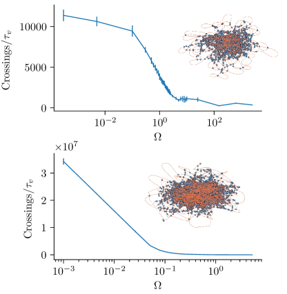
Figure 6: Number of times a trajectory crosses itself during one velocity correlation time vs. inertial parameter. Top: ISM, bottom: 2-$d$ stochastic harmonic oscillator. Insets show, as an example, the trajectories for $\Omega=1$ for each system, with circles indicating the intersections.

IV Discussion and conclusions

We have shown how the inertial spin model equations of motion must be modified to include position-dependent forces in this model. The most compact formulation is in terms of velocity and spin, Eqs. (18), where the positional forces enter only in the equation for the spin.

As a simple application of the new equations, we have considered a single harmonically confined active particle, and shown how inertia can be detected in this simple case without collective effects. The appearance of an anti-correlation minimum in the velocity temporal self-correlation function is an effect of strong confinement and it appears in over- and under-damped systems, but longer-lasting damped oscillations are only found with high inertia. Such damped oscillations were recently reported for male Anopheles gambiae (malaria mosquitoes) in laboratory swarms Cavagna et al. (2023b). Also, the trajectories recorded in that work look more “open” than the Vicsek trajectories, displaying loops roughly similar to the simulated trajectories at high $\Omega$ in Fig. 1. The present developments are useful for attempting to apply the ISM to the analysis of these and other experiments on laboratory-confined swarms (e.g. Ni et al. (2015); Gorbonos et al. (2016)).

As a next step, it is clearly of interest to study systems of many particles with open boundary conditions, maintaining a finite density through confinement or cohesive interactions. This can be done with the present formulation of the inertial spin model, and it is worth pursuing to achieve a better description of experimental results as well as to gain further theoretical understanding of the collective properties of active models. As an example, in a series of recent papers González-Albaladejo et al. (2023); González-Albaladejo and Bonilla (2023a, b), it has been claimed that, for the Vicsek model, replacing periodic boundaries with an harmonic confinement alters the behavior of the model near ordering, giving rise to a phase transition characterized by scale-free chaos and an extended criticality region and yielding different static and dynamic critical exponents. Open conditions thus deserve deeper inquiry, both for over- and under-damped inertial systems. Finally, position-dependent forces can also be used to investigate the response of a swarm to external perturbations that do not directly alter the velocities. Work in these directions is in progress.