DMS*: Minimizing Makespan for
Multi-Agent Combinatorial Path Finding
Abstract
Multi-Agent Combinatorial Path Finding (MCPF) seeks collision-free paths for multiple agents from their initial to goal locations, while visiting a set of intermediate target locations in the middle of the paths. MCPF is challenging as it involves both planning collision-free paths for multiple agents and target sequencing, i.e., solving traveling salesman problems to assign targets to and find the visiting order for the agents. Recent work develops methods to address MCPF while minimizing the sum of individual arrival times at goals. Such a problem formulation may result in paths with different arrival times and lead to a long makespan, the maximum arrival time, among the agents. This paper proposes a min-max variant of MCPF, denoted as MCPF-max, that minimizes the makespan of the agents. While the existing methods (such as MS*) for MCPF can be adapted to solve MCPF-max, we further develop two new techniques based on MS* to defer the expensive target sequencing during planning to expedite the overall computation. We analyze the properties of the resulting algorithm Deferred MS* (DMS*), and test DMS* with up to 20 agents and 80 targets. We demonstrate the use of DMS* on differential-drive robots.
Index Terms:
Path Planning for Multiple Mobile Robots or Agents, Multi-Agent Path Finding, Traveling Salesman ProblemI Introduction
Multi-Agent Path Finding (MAPF) seeks a set of collision-free paths for multiple agents from their respective start to goal locations. This paper considers a generalization of MAPF called Multi-Agent Combinatorial Path Finding (MCPF), where the agents need to visit a pre-specified set of intermediate target locations before reaching their goals. MAPF and MCPF arise in applications such as surveillance [1] and logistics [2]. For instance, factories [3, 4] use a fleet of mobile robots to visit a set of target locations to load machines for manufacturing. These robots share a cluttered environment and follow collision-free paths. In such settings, MAPF problems and their generalizations naturally arise to optimize operations.
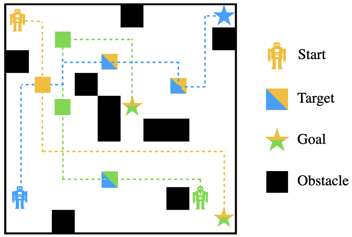
MCPF is challenging as it involves both collision avoidance among the agents as present in MAPF, and target sequencing, i.e., solving Traveling Salesman Problems (TSPs) [5, 6] to specify the allocation and visiting orders of targets for all agents. Both the TSP and the MAPF are NP-hard to solve to optimality [7, 5], and so is MCPF. A few methods have been developed [8, 9] to address the challenges in MCPF, and they often formulate the problem as a min-sum optimization problem, denoted as MCPF-sum, where the objective is to minimize the sum of individual arrival times. Such a formulation may result in an ensemble of paths where some agents arrive early while others arrive late, which leads to long execution times before all agents finish their paths. This paper thus proposes a min-max variant of MCPF (Fig. 1), denoted as MCPF-max, where the objective is to minimize the maximum arrival time, which is also called the makespan, of all agents.
To solve MCPF-max, this paper first adapts our prior MS* algorithm [8], which was first designed for MCPF-sum, to address MCPF-max. Then, we further develop two new techniques to expedite the planning, and we call the resulting new algorithm Deferred MS* (DMS*).
Specifically, the existing MS* follows the general heuristic search framework (such as A*) by iteratively generating, selecting and expanding states to construct partial solution paths from the initial state to the goal state. MS* uses Traveling Salesman Problem (TSP) algorithms to compute target sequences for agents. When solving the TSP, agent-agent collision are ignored, and the cost of resulting target sequences are thus lower bounds of the true costs for the agents to arrive at their goals. Therefore, the cost of target sequences provides an admissible heuristic to guide the state selection and expansion as in A*. Furthermore, MS* leverages the idea in M* [10] to first use the target sequences to build a low-dimensional search space, and then grow this search space by coupling agents together for planning only when collision happens. By doing so, MS* interleaves TSP (target sequencing) and MAPF (collision resolution) techniques under the heuristic search framework and is able to provide completeness and solution quality guarantees.
The first technique developed in this paper is applicable to MS* for both MCPF-max and MCPF-sum. When expanding a state, a set of successor states are generated, and for each of them, MS* needs to invoke the TSP solver to find the target sequence and the heuristic value of this successor state. Since the number of successor states can be large for each expansion, MS* needs to frequently invokes the TSP solver which slows down the computation. To remedy this issue, for each generated successor, we first use a fast-to-compute yet roughly estimated cost-to-go as the heuristic value, and defer calling TSP solver for target sequencing until that successor is selected for expansion.
The second technique developed in this paper is only applicable to MS* when solving MCPF-max, and does not work for MCPF-sum. Since the goal here is to minimize the makespan, during the search, agents with non-maximum arrival time naturally have “margins” in a sense that they can take a longer path without worsening the makespan of all agents. We take advantage of these margins to let agents re-use their previously computed target sequences and defer the expensive calls of TSP solvers until the margin depletes.
To verify the methods, we conduct both simulation in various maps with up to 20 agents and 80 targets, as well as real robot experiments. The simulation shows that the new techniques in DMS* help triple the success rates and reduce the average runtime to solution. The real robot experiments demonstrate that the planned path are executable on real robots, and that DMS* is able to optimize makespan while the existing planners that minimize the sum of arrival times can lead to long makespan.
II Related Work
II-A Multi-Agent Path Finding
To find collision-free paths for multiple agents, a variety of MAPF algorithms were developed, falling on a spectrum from coupled [11] to decoupled [12], trading off completeness and optimality for scalability. In the middle of this spectrum lie the dynamically-coupled methods such as M* [10] and CBS [13], which begin by planning for each agent a shortest path from the start to the goal ignoring any potential collision with the other agents, and then couple agents for planning only when necessary in order to resolve agent-agent collision. These dynamically-coupled methods were improved and extended in many ways [14, 15, 16, 17].
II-B Traveling Salesman Problems
In the presence of multiple intermediate targets, the planner needs to determine both the assignment and visiting order of the targets for the agents. For a single agent, the well-known Traveling Salesman Problem (TSP), which seeks a shortest tour that visits every vertex in a graph, is one of the most well-known NP-hard problems [5]. Closely related to TSP, the Hamiltonian Path Problem (HPP) requires finding a shortest path that visits each vertex in the graph from a start vertex to a goal vertex. The multi-agent version of the TSP and HPP (denoted as mTSP and mHPP, respectively) are more challenging since the vertices in the graph must be allocated to each agent in addition to finding the optimal visiting order of vertices. To simplify the presentation, we refer to all these problems simply as TSPs. To solve TSPs, a variety of methods have been developed ranging from exact methods (branch and bound, branch and price) [5] to heuristics [18] and approximation algorithms [19], trading off solution optimality for runtime efficiency. This work does not develop new TSPs solvers and leverage the existing ones.
II-C Target Assignment, Sequencing and Path Finding
Some recent research combines MAPF with target assignment and ordering [20, 21, 22, 23, 24, 25, 9, 8, 26, 27, 28, 29]. Most of them either consider target assignment only (without the need for computing visiting orders of targets) [20, 21, 22], or consider the visiting order only given that each agent is pre-allocated a set of targets [23, 24, 25]. Our prior work [8, 9] seeks to handle the challenge in target assignment and ordering as well as the collision avoidance in MAPF simultaneously. These work uses the MCPF-sum formulation and the developed planners minimize the sum of individual arrival times, while this paper investigates MCPF-max, which seeks to minimize the maximum arrival time.
III Problem
Let index set denote a set of agents. All agents share a workspace that is represented as an undirected graph , where stands for workspace. Each vertex represents a possible location of an agent. Each edge represents an action that moves an agent between and . maps an edge to its positive cost value. In this paper, the cost of an edge is equal to its traversal time, and each edge has a unit cost.111In [8, 9], the edge cost can be different from its traversal time: the edge cost can be any positive number while the traversal time is always one unit per edge. In this paper, the edge cost are the same as the edge traversal time, which is one for each edge.
Let the superscript over a variable denote the specific agent to which the variable belongs (e.g. means a vertex corresponding to agent ). Let denote the initial (or original) vertex and the goal (or destination) vertex of agent respectively. Let denote the set of all initial and goal vertices of the agents respectively, and let denote the set of target vertices. For each target , let denote the subset of agents that are eligible to visit ; these sets are used to formulate the (agent-target) assignment constraints.
Let denote a path for agent between vertices and , which is a list of vertices in with . Let denote the cost of the path, which is the sum of the costs of all edges present in the path: .
All agents share a global clock and start to move along their paths from time . Each action of the agents, either wait or move along an edge, requires one unit of time. Any two agents are in conflict if one of the following two cases happens. The first case is a vertex conflict where two agents occupy the same vertex at the same time . The second case is an edge conflict , where two agents go through the same edge from opposite directions between times and .
Definition 1 (MCPF-max Problem).
The Multi-Agent Combinatorial Path Finding with Min-Max Objective (MCPF-max) seeks to find a set of conflict-free paths for the agents such that (1) each target is visited222In MCPF-max, the notion that an agent “visits” a target means (i) there exists a time such that agent occupies along its path, and (ii) the agent claims that is visited. In other words, if a target is in the middle of the path of agent and agent does not claim is visited, then is not considered as visited. Additionally, a visited target can appear in the path of another agent. For the rest of the paper, when we say an agent or a path “visits” a target, we always mean the agent “visits and claims” the target. at least once by some agent in , (2) the path for each agent starts at its initial vertex and terminates at a unique goal vertex such that , and (3) the maximum of the cost of all agents’ paths (i.e., reaches the minimum.
IV Method
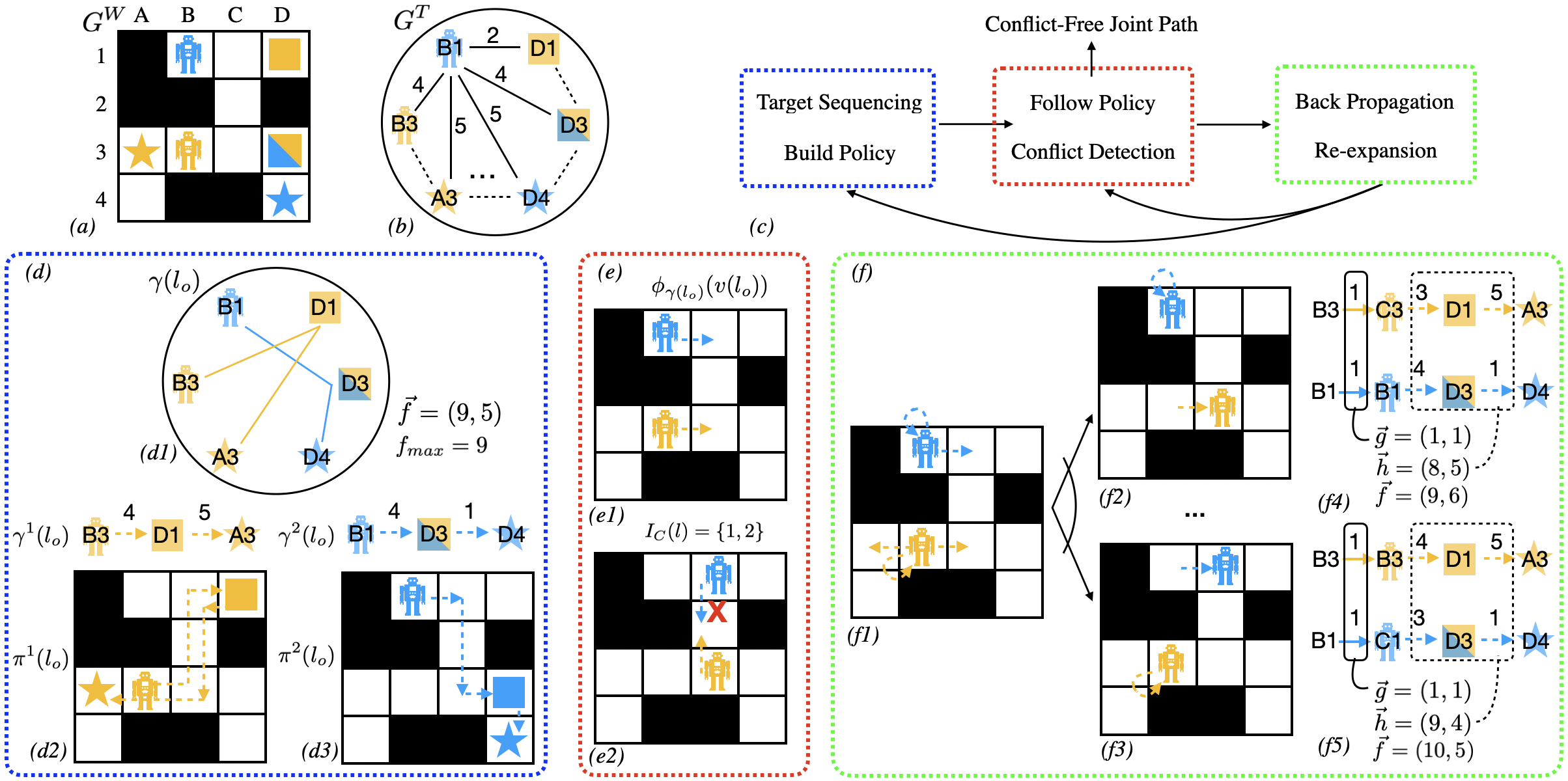
This section begins with a toy example in Fig. 2 to illustrate the planning process of DMS*, and provides the explanation in the caption. This section then introduces the concepts and notations, explains the pseudo-code and elaborates the technical detail.
IV-A Concepts and Notations
IV-A1 Joint Graph
Let denote the joint graph of all agents which is the Cartesian product of copies of , where each vertex represents a joint vertex and represents a joint edge that connects a pair of joint vertices. The joint vertex corresponding to the initial vertices of all agents is called the initial joint vertex. Let denote a joint path, which is a tuple of (individual) paths of the same length, i.e., . For the rest of this paper, we use a “path” to denote an “individual path”. DMS* searches the joint graph for a joint path that solves the MCPF-max.
IV-A2 Binary Vector
For any joint vertex , there can be multiple joint paths, e.g. , from to with different sets of targets visited along the joint path, and we need to differentiate between them during the search. We therefore introduce the following concepts. First, without losing generality, let all targets in be arranged as an ordered list , where subscript indicates the index of a target in this list.333In this paper, for a vector related to targets (e.g. a binary vector of length ), we use subscripts (e.g. ) to indicate the elements in the vector. For a vector or joint vertex that is related to agents (e.g. of length , or ), we use a superscript (e.g. in ) to indicate the element in the vector or joint vertex corresponding to an agent. Let denote a binary vector of length that indicates the visiting status of all targets in , where the -th component of is denoted as , and if the corresponding target is visited by some agent, and otherwise.
IV-A3 Label
Let denote a label, where is a joint vertex, is a binary vector of length , and is a cost vector of length . Here, each component corresponds to the path cost of agent . Intuitively, each label identifies a joint path from to that visits a subset of targets as described by and with path costs as specified by . To simplify the presentation, given a label , let denote the corresponding component in , and let denote the vertex of agent in , . Furthermore, let denote the maximum path cost over all agents in . To solve the MCPF-max in Def. 1, the algorithm needs to find a label , whose corresponding joint path leads all agents to visit all targets and eventually reach the goals, and is the objective value to be minimized.
IV-A4 Label Comparison
To compare two labels at the same joint vertex (i.e., to compare the joint paths represented by these two labels), we need to compare both their binary vectors as well as the path costs. We introduce the following dominance relationship to compare two binary vectors.
Definition 2 (Binary Dominance).
For any two binary vectors and , dominates (), if both the following conditions hold: (i) , ; (ii) , .
Intuitively, dominates if visits all targets that are visited in , and visits at least one more target than . In addition, two binary vectors are equal to each other () if both vectors are component-wise same to each other.
To compare two labels with the same joint vertex, we define the following dominance rule between them.
Definition 3 (Label Dominance).
For any two labels and with , dominates () if either of the following two conditions holds: (i) , ; (ii) , .
Intuitively, if dominates , then the joint path identified by is guaranteed to be better than the joint path identified by . If does not dominate , is then non-dominated by . Any two labels are non-dominated (with respect to each other) if each of them is non-dominated by the other. Two labels are said to be equal to (or same to) each other (notationally ) if they have the same vertex, binary vector and (i.e., ). Note that there is no need to compare and when comparing labels since the problem in Def. III seeks to minimize the maximum path cost over the agents. Finally, for each joint vertex , let denote a set of labels that are non-dominated to each other during the search.
IV-A5 Target Sequencing
Let denote an (individual) target sequence, where is the initial vertex of agent , each is a target vertex and is a goal vertex. A target sequence specifies both the assignment and visiting order of targets for agent . Let denote a joint sequence, which specify the assignment and visiting order of all targets for all agents.
Given a label , specifies the set of targets that are visited and unvisited. We introduce the notation , which is a joint sequence based on in the sense that visits all unvisited targets in . In other words, (i) each starts with , the vertex of agent in , visits a set of unvisited targets , where the -th component of is zero, and ends with a goal vertex ; (ii) all collectively visits all unvisited targets as specified in .
IV-A6 Target Graph
Let denote a minimum-cost path between in the workspace graph , and let denote the cost of path . The cost of a target sequence is equal to the sum of for any two adjacent vertices in .
Given a label , to find a joint sequence , a corresponding min-max multi-agent Hamiltonian path problem (mHPP) needs to be solved. Let SolveMHPP() denote a procedure that solves the mHPP. SolveMHPP() first formulates a target graph , which is computed based on the workspace graph as follows. The vertex set includes the current vertices of agents , the unvisited targets and goals . is fully connected and . The edge cost in of any pair of vertices is denoted as , which is the cost of a minimum cost path in the workspace graph . An example is shown in Fig. 2(b). The aforementioned target sequence for an agent is a path in and a joint sequence is a set of paths that starts from , visits all unvisited targets in as specified by , and ends at goals , while satisfying the assignment constraints. The procedure SolveMHPP can be implemented by various existing algorithms for mHPP.
IV-A7 Heuristic and Policy
Given a joint sequence , to simplify the notations, let be a heuristic value. Since agent-agent conflicts are ignored along the target sequences, the vector provides an estimate of the cost-to-go for each agent . When SolveMHPP() solves the mHPP to optimality, the corresponding provides lower bounds of the cost-to-go for all agents, which can be used as an admissible heuristic for the search. For any label , let be the -vector of , which is an estimated cost vector of the entire joint path from the initial vertices to goals for all agents by further extending the joint path represented by . Let denote the maximum component in , which provides an estimate of the objective value related to label .
Given a label and its joint sequence , a joint policy can be built out of , which maps one label to another label as follows. First, a joint path can be built based on by replacing any two subsequent vertices for any agent with a corresponding minimum cost path in . Then, along this joint path , all agents move from one joint vertex to , . A set of corresponding binary vectors for each can be built by first making , and then updating based on and by considering if visits any new targets. A set of corresponding cost vectors can also be computed in a similar way as by starting from . As a result, a joint policy is built by mapping one label to the next label along the target sequence . Given a vertex of agent , let denote the next vertex of agent in the joint policy . An example of is shown in Fig. 2(d). A label is called on-policy if its next label is known in for some . Otherwise, is called off-policy, which means its next label is unknown yet and a mHPP needs to be solved from to find the policy . We denote SolveMHPP() as the process of computing the joint sequence, heuristic values and joint policy.
IV-B DMS* Algorithm
To initialize (Lines 1-3), DMS* begins by creating an initial label and invokes the procedure SolveMHPP (as aforementioned) to compute for . For each label , DMS* uses two -values: and . Here, is a fast-to-compute yet roughly estimated cost-to-go, which does not require computing any joint sequence from to the goals. In contrast, is an estimated cost-to-go based on a joint sequence, which is computationally more expensive to obtain than . Similarly to A* [30], let OPEN denote a priority queue that stores labels and prioritizes them based on their -values from the minimum to the maximum. In Alg. 1, we point out which -value (either or ) is used when a label is added to OPEN. Finally, is added to since is non-dominated by any other labels at , and is added to OPEN for future search.444The notion of frontier set in this paper differs from the ones in . In , contains only expanded labels, which resembles the closed set in conventional A*, while in this paper, includes both the labels that are expanded (closed labels) and labels that are generated and not yet expanded (open labels).
In each search iteration (Lines 5-27), DMS* begins by popping a label from OPEN for processing. DMS* first calls the TargetSeq procedure for , which takes the parent label of (denoted as ), itself, and the conflict set of . TargetSeq determines either to call SolveMHPP to find a joint sequence for (i.e., ), or to re-use the joint sequence that is previously computed for as . We elaborate TargetSeq in Sec. IV-C. After TargetSeq on Line 7, the heuristic may change since a joint sequence may be computed for within TargetSeq, DMS* thus computes the and compare it against . When computing out of and on Line 8, a heuristic inflation factor is used, which scales each component in by the factor . Heuristic inflation is a common technique for A* [31] and M*-based algorithms [10] that can often expedite the computation in practice while providing a -bounded sub-optimal solution [31]. If , then should not be expanded in the current iteration since there can be labels in OPEN that have smaller -value than . DMS* thus updates to be , re-adds to OPEN with the updated , and skip the current search iteration. In a future search iteration, when this label is popped again, the condition on Line 9 will not hold since , and will be expanded.
Afterwards, DMS* checks if leads to a solution using CheckSuccess(), which verifies if every component in is one and if every component of is a unique goal vertex while satisfying the assignment constraints. If CheckSuccess() returns true, a solution joint path is found and can be reconstructed by iterative tracking the parent pointers of labels from to in Reconstruct(). DMS* then terminates.
If CheckSuccess() returns false, is expanded by considering its limited neighbors [10] described as follows. Let denote the conflict set of label , which is a subset of agents that are (or will be) in conflict. The limited neighbors of is a set of successor labels of . For each agent , if , agent is only allowed to move to its next vertex as defined in the joint policy . If , agent is allowed to visit any adjacent vertex of in . In other words, the successor vertices of are the following:
| (1) |
Let denote the set of successor vertices of , which is either of size one or equal to the number of edges incident on in . The successor joint vertices of is then the combination of for all , i.e., . For each joint vertex , a corresponding label is created and added to , the set of successor labels of . When creating , the corresponding and are computed based on and .
After generating the successor labels of , for each label , DMS* checks for conflicts between agents during the transition from to , and store the subset of agents in conflict in the conflict set . DMS* then invokes a procedure BackProp (Alg. 3) to back propagate to its ancestor labels recursively so that the conflict set of these ancestor labels are modified, and labels with modified conflict set are re-added to OPEN and will be re-expanded. DMS* maintains a back_set() for each label , which is a set of pointers pointing to the predecessor labels to which the back propagation should be conducted. Intuitively, similarly to [10, 8], the conflict set of labels are dynamically enlarged during planning when agents are detected in conflict. The conflict sets of labels determine the sub-graph within the joint graph that can be reached by DMS*, and DMS* always attempts to limit the search within a sub-graph of as small as possible.
Afterwards, if the conflict set is non-empty, then label leads to a conflict and is discarded. Otherwise, is checked for dominance against any existing labels in using Def. 3. If is dominated by or is equal to any existing labels in , is pruned, since any future joint path from can be cut and paste to a label that dominates without worsening the cost to reach goals. Furthermore, for each label that dominates or is equal to , the procedure DomBackProp(Alg. 4) is invoked so that the conflict set is back propagated to , and is added to the back_set of . By doing so, DMS* is able to keep updating the conflict set of the predecessor labels of after is pruned. This ensures that, when needed, the predecessor labels of will also be re-expanded after is pruned.
If label is not pruned, a procedure SimpleHeu is invoked for to quickly compute a heuristic that roughly estimates the cost-to-go. One possible way to implement SimpleHeu is to first copy , where is the parent of , and then reduce each component of the copied vector by one except for the components that are already zero. This heuristic is still an underestimate of the cost-to-go since all agents can move at most one step closer to their goals in each expansion. Then, the can be computed and is added to OPEN with as its priority. Other related data structure including , back_set, are also updated correspondingly, and the current search iteration ends.
When DMS* terminates, it either finds a conflict-free joint path, or returns failure when OPEN is empty if the given instance is unsolvable.
IV-C Deferred Target Sequencing
DMS* introduces two techniques to defer the target sequencing until absolutely needed. As aforementioned, the first one uses a fast-to-compute yet roughly estimated cost-to-go as the heuristic when a label is generated, and invokes TargetSeq only when that label is popped from OPEN for expansion.
We now focus on the second technique in DMS*. In the previous MS* [8], every time when the search encounters a new label that is off-policy, inside TargetSeq, the procedure SolveMHPP needs to be invoked for to find a joint sequence and policy from , which makes the overall computation burdensome, especially when a lot of new labels are generated due to the agent-agent conflict.
Different from MS*, DMS* seeks to defer the call of SolveMHPP inside TargetSeq. For a label , DMS* attempts to avoid calling SolveMHPP for by re-using the joint sequence of its parent label ( is the parent of ). As presented in Alg. 2, on Lines 5-6, DMS* first attemps to build a policy from by following the joint sequence of its parent label and computes the corresponding cost-to-go . Agents that are not in the conflict set (i.e., ) are still along their individual paths as specified by the previously computed policy . Agents that are in the conflict set (i.e., ) consider all possible actions as described in Equation (1) and may deviate from the individual paths specified by the previously computed policy . Therefore, DMS* needs to go through a check for these agents : DMS* first computes the -vector by summing up and . Then, if of some agent is no larger than , DMS* can avoid calling SolveMHPP, since letting the agents follow in the future will not worsen the objective value. Otherwise, there exists an agent , whose corresponding is greater than , and in this case, DMS* cannot avoid calling SolveMHPP since there may exists another joint sequence from , which leads to a solution joint path with better (smaller) objective value.
IV-D Properties of DMS*
IV-D1 Completeness
This section discusses the properties of DMS*. An algorithm is complete for a problem if finds a solution for solvable instances, and reports failure in finite time for unsolvable instances.
Theorem 1.
DMS* is complete for MCPF-max.
Let denote the set of all possible binary vectors and let denote the Cartesian of the joint graph and . is a finite space. DMS* uses dominance pruning and does not expand the same label twice during the search. As a result, for a unsolvable instance, DMS* enumerates all possible joint paths that starts from to any reachable and terminates in finite time. For a solvable instance, DMS* conducts systematic search in and returns a solution in finite time.
IV-D2 Solution Optimality
To discuss the solution optimality of DMS*, we needs the following assumptions.
Assumption 1.
The procedure SolveMHPP returns an optimal joint sequence for the given mHPP instance.
Theorem 2.
For a solvable instance, when Assumption 1 and 2 hold, DMS* returns an optimal solution joint path.
The proof of Theorem 2 follows the analysis in [10, 8], and we highlight the main ideas here. The policies computed by DMS* defines a sub-graph of the joint graph . DMS* first expands labels in this sub-graph . If no conflict is detected when following the policy, then the resulting joint path is conflict-free and optimal due to Assumption 1: With Assumption 1, for any label computed by SolveMHPP is an estimated cost-to-go that is admissible, i.e., is no larger than the true optimal cost-to-go. This is true because SolveMHPP ignores agent-agent conflicts and the resulting must be a lower bound on the true cost-to-go. As DMS* selects labels from OPEN in the same way as A* does, admissible heuristics lead to an optimal solution [31].
If conflicts are detected, DMS* updates (i.e., enlarges) by enlarging the conflict set and back propagating the conflict set. When Assumption 2 holds, the enlarged still ensures that an optimal conflict-free joint path is contained in the updated [10, 8]. DMS* systematically search over and finds at termination.
We now explain if Assumption 2 is violated, why DMS* loses the optimality guarantee and how to fix it. In MCPF-max, all agents are “coupled” in the space of binary vectors in a sense that a target visited by one agent does not need to be visited by any other agents. As as result, when one agent changes its target sequence by visiting some target that is previously assigned to another agent, all agents may need to be re-planned in order to ensure solution optimality. It means that, when Line 7 in Alg. 1 returns true for label , procedure SolveMHPP needs to be called for and SolveMHPP may return a new joint sequence . In this new sequence , it is possible that agents within visits targets that are previously assigned to agents that are not in . However, DMS* does not let agents outside to take all possible actions as defined in Equation (1). As a result, an optimal solution joint path may lie outside and DMS* thus loses the solution optimality guarantee when Assumption 2 is violated.
To ensure solution optimality when Assumption 2 is violated, same as in [8], one possible way is to back propagate the entire index set as the conflict set when calling BackProp. This ensures that DMS* considers all possible actions for all agents when conflicts between agents are detected. However, in practice, this is computationally burdensome when is large, and limits the scalability of the approach. We therefore omit it from Alg. 1 for clarity.
IV-D3 Solution Bounded Sub-Optimality
A joint sequence is -bounded sub-optimal () if , where is an optimal joint sequence. Similarly, a solution joint path is -bounded sub-optimal if its objective value , where is the true optimum of the given instance.
Theorem 3.
For a solvable instance, if (i) SolveMHPP returns a -bounded sub-optimal joint sequence for any given label and (ii) Assumption 2 holds, then DMS* returns a -bounded solution joint path.
Bounded sub-optimal joint sequences lead to inflated heuristic values for labels in DMS*. As DMS* select labels based on -values as A* does, inflated heuristic values lead to bounded sub-optimal solutions for the problem [31].
In addition to using bounded sub-optimal joint sequences, DMS* is also able to use the conventional heuristic inflation technique [31] and provide bounded sub-optimal solution.
V Experimental Results
We implement DMS* in Python, and use Google OR-Tool555https://developers.google.com/optimization/routing/routing_tasks as the mHPP solver, which implements the SolveMHPP procedure that is required by DMS*. Limited by our knowledge on Google OR-Tool, we only consider the following type of assignment constraints, where any agent can visit all targets and goals. We use grid maps from the MAPF benchmark data set [32] and set up a 60-second runtime limit for each test instance, where each test instance contains the starts, targets and goals, which are all from the MAPF benchmark data set [32]. All tests run on a MacBook Pro with a Apple M2 Pro CPU and 16GM RAM. It is known from [10] that, for M*-based algorithms, a slightly inflated heuristic can often help improve the scalability of the approach with respect to the number of agents and we set in our tests. We set the number of targets in our tests. We compare DMS*, which includes the two proposed technique to defer target sequencing, against MS*, which is the baseline and does not have these two techniques. In other words, MS* here is a naive adaption of the existing MS* [8] algorithm to solve MCPF-max, by using the aforementioned Google OR-Tool to solve min-max mHPP for target sequencing.
V-A Varying Number of Agents
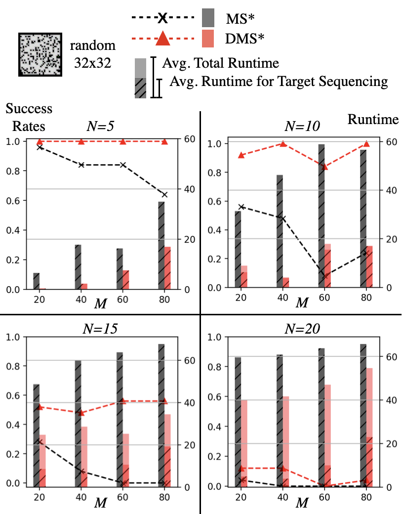
We first fix the map to be Random 32x32, and vary the number of agents . We measure the success rates, the average runtime to solution and the average runtime for target sequencing per instance. The averages are taken over all instances, including both succeeded instances and instances where the algorithm times out. As shown in Fig. 3, DMS* achieves higher success rates and lower runtime than the baseline MS* for all s. As increases from to , both algorithms require more runtime for target sequencing. As increases from to , agents have higher density and are more likely to run into conflict with each other. As a result, both algorithms time out for more and more instances. Additionally, MS* spends almost all of its runtime in target sequencing, which indicates the computational burden caused by the frequent call of mHPP solver. In contrast, for DMS*, when , DMS* spends most of the runtime in target sequencing, while as increases to , DMS* spends more runtime in path planning.
V-B Different Maps
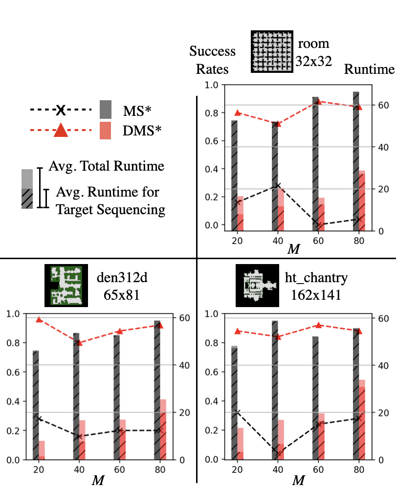
We then fixed the number of agents to and test both algorithms in several maps of different sizes, as shown in Fig. 4. DMS* outperforms MS* in terms of success rates due to the alleviated computational burden for target sequencing. Furthermore, larger maps do not lead to lower success rates since larger maps can reduce the density of the agents and make the agents less likely to run into conflicts with each other. The Room 32x32 map is relatively more challenging than the other two maps since there are many narrow corridors which often lead to conflicts between the agents.
V-C Experiments with Mobile Robots
We also performed experiments with Husarion ROSbot 2666https://husarion.com/manuals/rosbot/, which are differential drive robots equipped with an ASUS Tinker Board and use a 2D lidar for localization. We used two such robots to perform tests in two different environments, as shown in Fig. 5 (a) and (b) having 2 and 3 targets, respectively. This test verifies that the paths planned by DMS* are executable on real robots. When the robots have large motion disturbance, such as delay or deviation from the planned path, additional techniques (such as [33]) will be needed to ensure collision-free execution of the paths, which is another research topic and is not the focus of this work. In our experiments, the robots run in slow speed and the motion disturbance of the robots are relatively small.

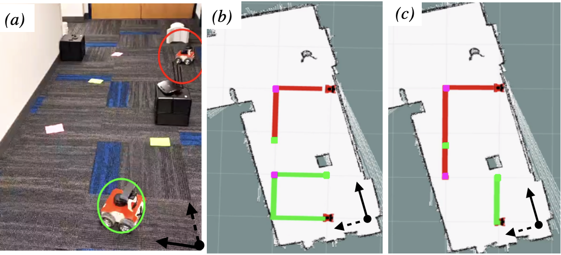
We then compare the performance of DMS* (which minimizes the makespan) and MS* (which minimizes the sum of arrival times) on the mobile robots. Both planners were tested on the same map with two intermediate targets as shown in Fig. 6. We observe that DMS* tends to distribute the targets evenly to the agents and plan paths to minimize the makespan, while MS* finds a solution wherein one robot visits all targets, and the other robot directly goes to its assigned destination. MS* seeks to minimize the sum of arrival times, which can lead to a large makespan.
VI Conclusion and Future Work
This paper investigates a min-max variant of Multi-Agent Combinatorial Path Finding problem and develops DMS* algorithm to solve this problem. We analyze the properties of DMS* and test DMS* with up to 20 agents and 80 targets. We also conduct robot experiments to showcase the usage of DMS* on differential-drive robots.
For future work, one can investigate how to incorporate the existing conflict resolution techniques for MAPF into the DMS* to further improve its runtime efficiency. We also note from our robot experiments that, the uncertainty and disturbance in robot motion may affect the execution of the planned path, and one can develop fast online replanning version of DMS* to address the uncertainty and disturbance.
Acknowledgments
This material is based upon work supported by the National Science Foundation under Grant No. 2120219 and 2120529. Any opinions, findings, and conclusions or recommendations expressed in this material are those of the author(s) and do not necessarily reflect the views of the National Science Foundation.
References
- [1] J. Keller, D. Thakur, M. Likhachev, J. Gallier, and V. Kumar, “Coordinated path planning for fixed-wing uas conducting persistent surveillance missions,” IEEE Transactions on Automation Science and Engineering, vol. 14, no. 1, pp. 17–24, 2016.
- [2] P. R. Wurman, R. D’Andrea, and M. Mountz, “Coordinating hundreds of cooperative, autonomous vehicles in warehouses,” AI magazine, vol. 29, no. 1, pp. 9–9, 2008.
- [3] M. Schneier, M. Schneier, and R. Bostelman, Literature review of mobile robots for manufacturing. US Department of Commerce, National Institute of Standards and Technology …, 2015.
- [4] K. Brown, O. Peltzer, M. A. Sehr, M. Schwager, and M. J. Kochenderfer, “Optimal sequential task assignment and path finding for multi-agent robotic assembly planning,” in 2020 IEEE International Conference on Robotics and Automation (ICRA), 2020, pp. 441–447.
- [5] D. L. Applegate, R. E. Bixby, V. Chvatal, and W. J. Cook, The Traveling Salesman Problem: A Computational Study (Princeton Series in Applied Mathematics). Princeton, NJ, USA: Princeton University Press, 2007.
- [6] T. Bektas, “The multiple traveling salesman problem: an overview of formulations and solution procedures,” omega, vol. 34, no. 3, pp. 209–219, 2006.
- [7] J. Yu and S. M. LaValle, “Structure and intractability of optimal multi-robot path planning on graphs,” in Twenty-Seventh AAAI Conference on Artificial Intelligence, 2013.
- [8] Z. Ren, S. Rathinam, and H. Choset, “MS*: A new exact algorithm for multi-agent simultaneous multi-goal sequencing and path finding,” in 2021 IEEE International Conference on Robotics and Automation (ICRA). IEEE, 2021.
- [9] ——, “Cbss: A new approach for multiagent combinatorial path finding,” IEEE Transactions on Robotics, vol. 39, no. 4, pp. 2669–2683, 2023.
- [10] G. Wagner and H. Choset, “Subdimensional expansion for multirobot path planning,” Artificial Intelligence, vol. 219, pp. 1–24, 2015.
- [11] T. S. Standley, “Finding optimal solutions to cooperative pathfinding problems,” in Twenty-Fourth AAAI Conference on Artificial Intelligence, 2010.
- [12] D. Silver, “Cooperative pathfinding.” 01 2005, pp. 117–122.
- [13] G. Sharon, R. Stern, A. Felner, and N. R. Sturtevant, “Conflict-based search for optimal multi-agent pathfinding,” Artificial Intelligence, vol. 219, pp. 40–66, 2015.
- [14] E. Boyarski, A. Felner, R. Stern, G. Sharon, D. Tolpin, O. Betzalel, and E. Shimony, “Icbs: improved conflict-based search algorithm for multi-agent pathfinding,” in Twenty-Fourth International Joint Conference on Artificial Intelligence, 2015.
- [15] L. Cohen, T. Uras, T. S. Kumar, and S. Koenig, “Optimal and bounded-suboptimal multi-agent motion planning,” in Twelfth Annual Symposium on Combinatorial Search, 2019.
- [16] Z. Ren, S. Rathinam, and H. Choset, “Loosely synchronized search for multi-agent path finding with asynchronous actions,” in 2021 IEEE/RSJ International Conference on Intelligent Robots and Systems. IEEE, 2021.
- [17] ——, “A conflict-based search framework for multiobjective multiagent path finding,” IEEE Transactions on Automation Science and Engineering, pp. 1–13, 2022.
- [18] K. Helsgaun, “General k-opt submoves for the lin–kernighan tsp heuristic,” Mathematical Programming Computation, vol. 1, no. 2, pp. 119–163, 2009.
- [19] N. Christofides, “Worst-case analysis of a new heuristic for the travelling salesman problem,” Carnegie-Mellon Univ Pittsburgh Pa Management Sciences Research Group, Tech. Rep., 1976.
- [20] W. Hönig, S. Kiesel, A. Tinka, J. Durham, and N. Ayanian, “Conflict-based search with optimal task assignment,” in Proceedings of the International Joint Conference on Autonomous Agents and Multiagent Systems, 2018.
- [21] H. Ma and S. Koenig, “Optimal target assignment and path finding for teams of agents,” in Proceedings of the 2016 International Conference on Autonomous Agents & Multiagent Systems, 2016, pp. 1144–1152.
- [22] V. Nguyen, P. Obermeier, T. C. Son, T. Schaub, and W. Yeoh, “Generalized target assignment and path finding using answer set programming,” in Twelfth Annual Symposium on Combinatorial Search, 2019.
- [23] P. Surynek, “Multi-goal multi-agent path finding via decoupled and integrated goal vertex ordering,” in Proceedings of the International Symposium on Combinatorial Search, vol. 12, no. 1, 2021, pp. 197–199.
- [24] H. Zhang, J. Chen, J. Li, B. C. Williams, and S. Koenig, “Multi-agent path finding for precedence-constrained goal sequences,” in Proceedings of the 21st International Conference on Autonomous Agents and Multiagent Systems, 2022, pp. 1464–1472.
- [25] X. Zhong, J. Li, S. Koenig, and H. Ma, “Optimal and bounded-suboptimal multi-goal task assignment and path finding,” in 2022 International Conference on Robotics and Automation (ICRA). IEEE, 2022, pp. 10 731–10 737.
- [26] H. Ma, J. Li, T. K. S. Kumar, and S. Koenig, “Lifelong multi-agent path finding for online pickup and delivery tasks,” in Conference on Autonomous Agents & Multiagent Systems, 2017.
- [27] M. Liu, H. Ma, J. Li, and S. Koenig, “Task and path planning for multi-agent pickup and delivery,” in 2019 AAMAS, 2019, pp. 1152–1160.
- [28] Q. Xu, J. Li, S. Koenig, and H. Ma, “Multi-goal multi-agent pickup and delivery,” in 2022 IEEE/RSJ International Conference on Intelligent Robots and Systems (IROS). IEEE, 2022, pp. 9964–9971.
- [29] C. Henkel, J. Abbenseth, and M. Toussaint, “An optimal algorithm to solve the combined task allocation and path finding problem,” arXiv preprint arXiv:1907.10360, 2019.
- [30] P. E. Hart, N. J. Nilsson, and B. Raphael, “A formal basis for the heuristic determination of minimum cost paths,” IEEE Transactions on Systems Science and Cybernetics, vol. 4, no. 2, pp. 100–107, 1968.
- [31] J. Pearl, Heuristics: intelligent search strategies for computer problem solving. Addison-Wesley Longman Publishing Co., Inc., 1984.
- [32] R. Stern, N. Sturtevant, A. Felner, S. Koenig, H. Ma, T. Walker, J. Li, D. Atzmon, L. Cohen, T. Kumar et al., “Multi-agent pathfinding: Definitions, variants, and benchmarks,” arXiv preprint arXiv:1906.08291, 2019.
- [33] W. Hönig, T. S. Kumar, L. Cohen, H. Ma, H. Xu, N. Ayanian, and S. Koenig, “Multi-agent path finding with kinematic constraints,” in Twenty-Sixth International Conference on Automated Planning and Scheduling, 2016.