Activation Gradient based Poisoned Sample Detection Against Backdoor Attacks

Abstract

This work focuses on defending against the data poisoning based backdoor attacks, which bring in serious security threats to deep neural networks (DNNs). Specifically, given a untrustworthy training dataset, we aim to filter out potential poisoned samples, i.e., poisoned sample detection (PSD). The key solution for this task is to find a discriminative metric between clean and poisoned samples, even though there is no information about the potential poisoned samples ($e.g.$, the attack method, the poisoning ratio). In this work, we develop an innovative detection approach from the perspective of the gradient w.r.t. activation (i.e., activation gradient direction, AGD) of each sample in the backdoored model trained on the untrustworthy dataset. We present an interesting observation that the circular distribution of AGDs among all samples of the target class is much more dispersed than that of one clean class. Motivated by this observation, we firstly design a novel metric called Cosine similarity Variation towards Basis Transition (CVBT) to measure the circular distribution’s dispersion of each class. Then, we design a simple yet effective algorithm with identifying the target class(es) using outlier detection on CVBT scores of all classes, followed by progressively filtering of poisoned samples according to the cosine similarities of AGDs between every potential sample and a few additional clean samples. Extensive experiments under various settings verify that given very few clean samples of each class, the proposed method could filter out most poisoned samples, while avoiding filtering out clean samples, verifying its effectiveness on the PSD task. Codes are available at https://github.com/SCLBD/bdzoo2/blob/dev/detection_pretrain/agpd.py.

1 Introduction

It is well known that deep neural networks (DNNs) are vulnerable to backdoor attacks [37], where the adversary could inject a particular backdoor into the DNN model through manipulating the training dataset or training process. Consequently,the backdoored model will produce a target label when encountering a particular trigger pattern, leading to unexpected security threats in practice. Protecting DNNs from backdoor attacks is an urgent and important task.

Here we focus on defending against the data-poisoning based backdoor attacks through filtering out the potential poisoned samples from a untrustworthy training dataset, i.e., poisoned sample detection (PSD). One of the main challenges for PSD is the information lack of the potential poisoned samples, such as the trigger type, the target class(es), the number of poisoned samples, etc.. Some seminal works have been developed by exploring some discriminative metrics based on the intermediate activation or predictions of poisoned and clean samples in the backdoored model trained on the untrustworthy dataset, such as activation clustering (AC) [21], STRIP [10], SCAn [31]. However, these metrics may fail under some particular settings. For example, the assumption of AC that there are two activation clusters in the target class and the smaller one correspond to poisoned samples would fail when the poisoning ratio is high, as verified in later experiments.

In this work, we develop a stable and effective detection approach in various attack settings, according to a novel perspective of the gradient w.r.t. activation (i.e., activation gradient direction, AGD), dubbed Activation Gradient based Poisoned Detection (AGPD). The behind motivation is based on the observation that a backdoored model tends to map poisoned and clean samples in the target class to similar areas in its feature space [14], such that they can be predicted as the same label, no matter what kind of backdoor attacks. Considering the significant discrepancy between poisoned and clean samples in their original space, their mapping directions should be significantly different. To verify this assertion, we investigate the AGD of one sample, which could reflect the sample’s mapping direction. Moreover, we define a novel concept called gradient circular distribution (GCD), which capture the distribution of all AGDs in one class. As shown in Fig. 1, we further observe that the GCD of a target class (containing both poisoned and clean samples) is much more dispersed than that of a clean class, which is stably observed across various backdoor attacks, settings, and datasets (see Supplementary Material). To quantitatively measure the GCD’s dispersion of one class, we design a novel metric called Cosine similarity Variation towards Basis Transition (CVBT). Given one class of samples, CVBT requires one or a few additional clean samples to serve as the basis vector of AGDs, such that the cosine similarities between all samples and this basis vector could be calculated. Then, the AGD of the sample with the smallest cosine similarity is determined as the far-end basis vector, to which the similarities of all samples are also calculated. The CVBT metric measures the variation between two similarities of all samples in one class. A larger CVBT score indicates a more dispersed class, and vice versa. Extensive experiments in various settings ($e.g.$, model architecture, dataset, attack method, poisoning ratio) verify the stable and strong discrimination of the CVBT metric. Then, based on the CVBT scores of all classes, the target class(es) could be accurately identified via outlier detection, followed by a progressive process to gradually filter out poisoned samples from the identified target class.

The main contributions of this work are three-fold. (1) We are the first to reveal the interesting observation that the GCD of the target class is more dispersed than that of the clean class, and design a novel metric to measure the GCD’s dispersion. (2) Utilizing the dispersion metric, we develop an innovative method by sequentially identifying the target class(es) and filtering poisoned samples for the poisoned sample detection task. (3) Extensive evaluations and analysis verify the superiority of the proposed method.

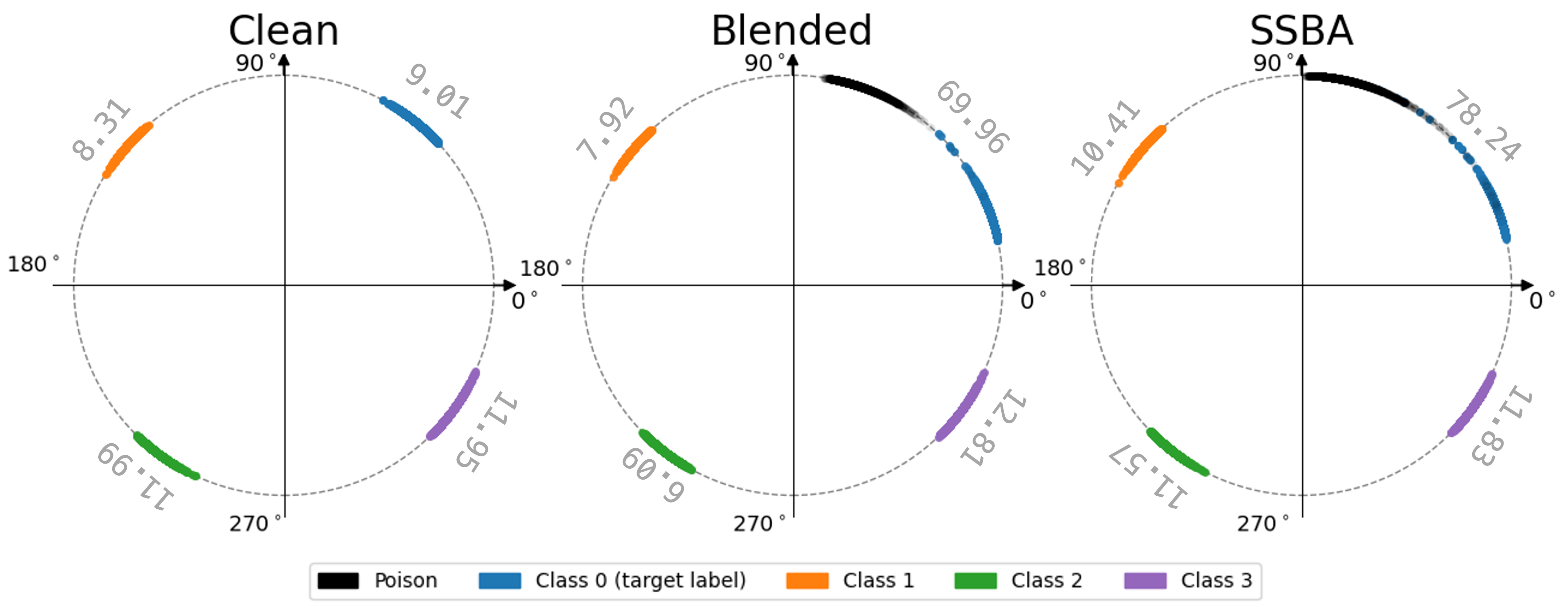
Figure 1: Gradient circular distributions (GCDs) across four classes of CIFAR-10, on the clean model (left), Blended attacked model (middle), and SSBA attacked model (right), respectively. The value along with each arc indicates the CVBT score, which measures its dispersion. The GCD of the target class (covering both black and blue arcs) is much more dispersed than those of three clean classes, on all three models. Note that we moved three clean classes’ arcs to different quadrants to avoid visual overlap.

2 Related Work

Backdoor Attack.

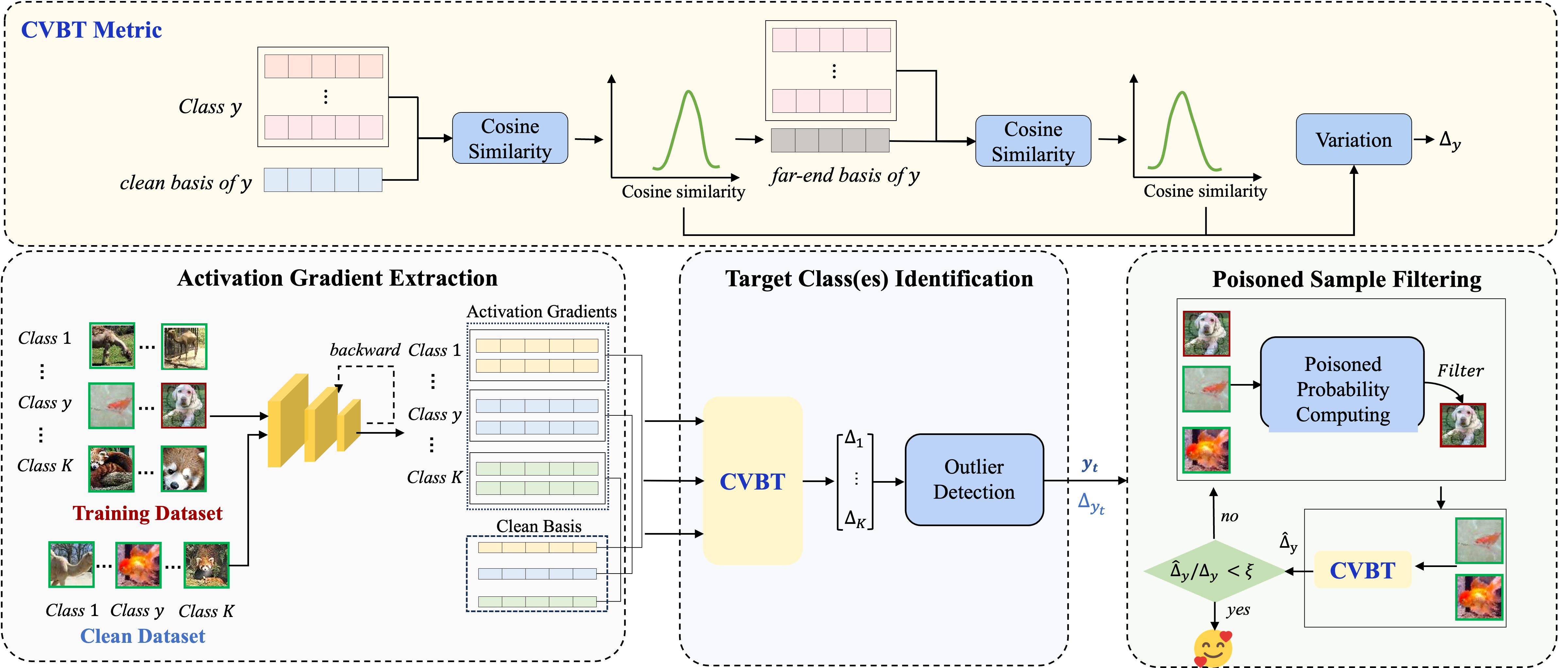
Figure 2: The illustrations of the proposed CVBT metric, and the pipeline of the proposed APGD method, including activation gradient extraction, layer selection and target class identification, and poisoned sample filtering.

Badnet  [12] is the first work to introduce how to insert a backdoor into DNNs, where the adversary manipulates training samples by adding a small path with particular patterns, and also change their labels to a target label. After this work, the trigger style becomes more diverse, such as a Hello kitty image or a random noise image used in Blended  [6], the universal adversarial perturbation with only low frequency components used in Low-Frequency  [39], and the sinusoidal signal used in SIG [2], etc.. One commonality of these triggers is that they are sample-agnostic, i.e., they are same across different poisoned samples. This characteristic is often leveraged to detect and remove the trigger or the poisoned sample. Thus, some sample agnostic triggers are designed, such as WaNet  [25], Input-Aware  [26], and SSBA  [18], Poison ink [41], LIRA [8], SleeperAgent [30]. However, poisoned samples with these triggers can also be distinguished from clean samples in the activation space. To tack it, the targeted contamination attack called TaCT [31] designs a source-specific trigger to make the poisoned sample activation less distinguishable from the clean sample activation. In addition to designing different types of triggers, some attacks also explore more settings of the numbers of triggers and target classes. Except of the regular all-to-one setting with one trigger and one target class, there are also all-to-all setting with one trigger and multiple target classes ($e.g.$, BadNets-A2A [12]), as well as multi-target and multi-trigger setting ($e.g.$, c-BaN [28], Marksman [9]). These various settings further increase the difficulty for poisoned sample detection.

Backdoor Defense.

According to the accessible information, several different branches of backdoor defense methods have been developed, such as the pre-training backdoor defense ($e.g.$, [21, 32, 1]) if given a untrustworthy training dataset, in-training backdoor defense ($e.g.$, [14, 19, 5, 23, 11]) if the training process can be controlled by defender, as well as post-training backdoor defense ($e.g.$, [20, 45, 44, 35, 34, 38, 40, 43, 4, 42]) if given a backdoored model. Due to the space limit, in the following we only review existing methods of poisoned sample detection (PSD), belonging to the pre-training backdoor defense. One general idea of most existing PSD methods is constructing some discriminative metrics between poisoned and clean samples based on the intermediate activation or final predictions of a backdoored model that is trained on the untrustworthy dataset. For example, the activation clustering (AC) [21] method assumes that the sample activation of the target class will form two clusters, and the smaller cluster corresponds to poisoned samples, while those of clean classes form one cluster. Spectral [32] assumes that the activation distributions of benign and poisoned samples in the target class are spectrally separable. Then, the poisoned samples can be identified through analyzing the spectrum of the covariance matrix of sample activation. Beatrix  [22] assumes that poisoned and clean samples are distinguishable in the Gramian activation space, which captures both the activation and activation correlation across neurons. Then, the poisoned samples are identified through out-of-distribution detection based on the Gram matrix. SCAn [31] assumes that the activation of each sample can be decomposed into two independent components, including a class-specific identity and a variation component, and the variation components of all clean samples follow the distribution, while not the case for poisoned samples. STRIP  [10] and SantiNet  [7] assume that if the input sample is perturbed, then the prediction of the poisoned sample will be more stable than that of the clean sample. In addition to above activation-based detection methods, FREAK [1] presents another frequency-based approach that poison samples have large gradients w.r.t. some particular frequency components, while benign samples have smaller gradients w.r.t. these components.

3 Methodology

3.1 Problem Formulation

Threat Model.

Consider a $K$-class classification problem with sample $\bm{x}\in\mathcal{X}$ and label $y\in[K]$. We assume that a potentially poisoned dataset $\mathcal{D}_{bd}$ of $N$ samples is accessible, which can be divided into two parts, i.e., the clean subset $\mathcal{D}_{c}$ and the poisoned part $\mathcal{D}_{p}$. Let the target class of the poisoned sample be $y_{t}$ and we denote the poisoned sample by $\tilde{\bm{x}}$. Then, a classifier trained on $\mathcal{D}_{bd}$ would perform normally on benign samples while predicting the target class $y_{t}$ for poisoned samples. We define the poisoning ratio $\beta=\frac{|\mathcal{D}_{p}|}{|\mathcal{D}_{bd}|}$ as the proportion of the poisoned samples in the whole training dataset.

Defender’s Goal.

We assume that the defender has access to both the potentially poisoned dataset $\mathcal{D}_{bd}$ and a small additional clean dataset $\mathcal{D}_{ac}$. We assume that the defender can train or access a model $f_{\bm{\theta}}:\mathcal{X}\to\mathbb{R}^{K}$ with model parameters $\bm{\theta}$, which maps input samples to $K$-dimensional logit vectors. The defender aims to filter out the potential poisoned samples from the dataset $\mathcal{D}_{bd}$, to prevent the backdoor injection during the training process.

3.2 Activation Gradient and Gradient Circular Dispersion

Activation Gradient.

For a sample $\bm{x}$ with label $y$, we denote its activation at $l$-th layer as $\bm{h}^{(l)}_{\bm{x}}\in\mathbb{R}^{C^{(l)}\times H^{(l)}\times W^{(l)}}$, where $C^{(l)}$, $H^{(l)}$, $W^{(l)}$ are the depth (number of channel), height and width of the $l$-th layer activation, respectively. Then, the channel-wise activation gradient, dubbed activation gradient $\bm{g}^{(l)}_{\bm{x}}\in\mathbb{R}^{C^{(l)}}$ is defined to be

$$\bm{g}^{(l)}_{\bm{x}}=\frac{1}{H^{(l)}W^{(l)}}\sum_{h=1}^{H^{(l)}}\sum_{w=1}^{W^{(l)}}\frac{\partial[f_{\bm{\theta}}(\bm{x})]_{y}}{\partial{[\bm{h}^{(l)}_{\bm{x}}]_{:,h,w}}},$$ (1)

where $[f_{\bm{\theta}}(\bm{x})]_{y}$ is the logit for class $y$ of sample $\bm{x}$ and $[\bm{h}^{(l)}_{\bm{x}}]_{:,h,w}\in\mathbb{R}^{C^{(l)}}$ is the activation sliced at height $h$ and width $w$ over all channels. To simplicity, hereafter we will use ‘gradient’ as a substitute for activation gradient.

Dispersion Metric.

To characterize the poisoned samples, we first provide the following definition:

Definition 1 (Gradient Circular Dispersion).

Define circular distribution as the probabilistic distribution $\mathcal{P}$ of the angle variable ranged over $[0,2\pi)$. Similarly, given a basis vector $g$, the Gradient Circular Distribution is defined as the circular distribution of angles between the activation gradients of a set of samples and the basis vector. Then, the Gradient Circular Dispersion (GCD) describes the spread of angles over the gradient circular distribution.

As illustrated in Section 1 and Fig. 1, we discover that the gradient circular dispersion of the target class is larger than the clean class, which motivates us to leverage the GCD to identify the target class(es). To quantify the GCD of each class, we propose a simple metric based on cosine similarity, dubbed Cosine similarity Variation towards Basis Transition (CVBT). Particularly, for the benign dataset $\mathcal{D}_{ac}$, we first compute the activation gradients of $\mathcal{D}_{ac}$ at layer $l$ by the backdoor model $f_{\bm{\theta}}$ trained on $\mathcal{D}_{bd}$ as Eq. (1) and obtain the clean basis for each class $y$ as follows:

$$\bar{\bm{g}}_{\mathcal{D}_{ac}^{y}}^{(l)}=\frac{1}{|\mathcal{D}_{ac}^{y}|}\sum_{\bm{x}\in\mathcal{D}_{ac}^{y}}\bm{g}^{(l)}_{\bm{x}},$$ (2)

where $\mathcal{D}_{ac}^{y}$ is the subset of $\mathcal{D}_{ac}$ containing all samples from class $y$. Then, the cosine similarity between samples from $\mathcal{D}_{bd}$ and the clean basis corresponding to their classes are calculated as follows:

$$s(\bm{x},\mathcal{D}_{ac}^{y};f_{\bm{\theta}},l)=\frac{\langle\bm{g}^{(l)}_{\bm{x}},\bar{\bm{g}}_{\mathcal{D}_{ac}^{y}}^{(l)}\rangle}{\|\bm{g}^{(l)}_{\bm{x}}\|\|\bar{\bm{g}}_{\mathcal{D}_{ac}^{y}}^{(l)}\|}.$$ (3)

Then, for each class $y$, the samples with the lowest cosine similarity form the suspected set $\mathcal{D}_{sus}^{y}$, which may contain one or multiple samples in practical calculation. The far-end basis is defined as $\bar{\bm{g}}_{\mathcal{D}_{sus}^{y}}^{(l)}$ calculated as did in Eq. (2). Consequently, the cosine similarity between samples and their corresponding far-end basis is calculated as follows:

$$s(\bm{x},\mathcal{D}_{sus}^{y};f_{\bm{\theta}},l)=\frac{\langle\bm{g}^{(l)}_{\bm{x}},\bar{\bm{g}}_{\mathcal{D}_{sus}^{y}}^{(l)}\rangle}{\|\bm{g}^{(l)}_{\bm{x}}\|\|\bar{\bm{g}}_{\mathcal{D}_{sus}^{y}}^{(l)}\|}.$$ (4)

Finally, given $\mathcal{D}_{bd}^{y}$, the CVBT metric for class $y$ at layer $l$ is defined to measure the cosine similarity variation according to between clean basis and far-end basis, as follows:

$$\Delta_{y}^{(l)}=\sqrt{\sum_{\bm{x}\in\mathcal{D}_{bd}^{y}}(s(\bm{x},\mathcal{D}_{ac}^{y};f_{\bm{\theta}},l)-s(\bm{x},\mathcal{D}_{sus}^{y};f_{\bm{\theta}},l))^{2}}.$$ (5)

Algorithm 1 Activation Gradient-based Poisoned sample Detection (AGPD).

0:  A untrustworthy dataset $\mathcal{D}_{bd}$, an additional clean dataset $\mathcal{D}_{ac}$, and a model $f_{\bm{\theta}}$ trained on $\mathcal{D}_{bd}$, and $p,\tau,\xi$

0:  Suspected set $\hat{\mathcal{D}}_{p}$ and purified set $\mathcal{D}_{bd}\backslash\hat{\mathcal{D}}_{p}$

1:  # Target Class(es) Identification

2:  for layer $l$ in $\{1,\dots,L\}$ do

3:     for class $y$ in $\{0,\dots,K-1\}$ do

4:        Compute CVBT $\Delta_{y}^{(l)}$ for class $y$ at layer $l$

5:     end for

6:     Calculate Z-score $z^{(l)}_{y}$ via Eq. (6)

7:     Record the anomaly score $z^{(l)}_{\max}=\max_{y}z^{(l)}_{y}$

8:  end for

9:  Choose the layer $l^{\prime}=\arg\max z^{(l)}_{\max}$

10:  Identify the target class(es) $Y_{t}=\{y\mid z^{(l^{\prime})}_{y}\geq p\}$

11:  # Poisoned Sample Filtering

12:  Set $\hat{\mathcal{D}_{p}}=\emptyset$.

13:  Compute CVBT $\hat{\Delta}_{y}^{(l)}$ for $\mathcal{D}^{y}_{bd}$ according to Eq. (5)

14:  for $y^{\prime}$ in $Y_{t}$ do

15:     repeat

16:        $\mathcal{D}^{y^{\prime}}_{bd}=\{(\bm{x},y)\mid(\bm{x},y)\in\mathcal{D}_{bd}\backslash\hat{\mathcal{D}}_{p},y=y^{\prime}\}$

17:        Compute the poisoned score $r(\bm{x})$ for each sample $\bm{x}$ in $\mathcal{D}^{y^{\prime}}_{bd}$ according to Eq. (7), and normalize it to $r^{\prime}(\bm{x})$

18:        Filter out the samples with $r^{\prime}(\bm{x})$ higher than $\tau$, and update the suspected dataset by $\hat{\mathcal{D}}_{p}\leftarrow\hat{\mathcal{D}}_{p}\cup\{(\bm{x},y)\mid r^{\prime}(\bm{x})\geq\tau,(\bm{x},y)\in\mathcal{D}^{y^{\prime}}_{bd}\}$

19:        Update $\hat{\Delta}_{y}^{(l)}$ according to Eq. (5) by replacing $\mathcal{D}^{y}_{bd}$ by $\mathcal{D}^{y}_{bd}\backslash\hat{\mathcal{D}}_{p}$

20:     until $\hat{\Delta}_{y}^{(l)}/\Delta_{y}^{(l)}\leq\xi$

21:  end for

3.3 Proposed Method

As shown in Fig. 2, the pipeline of our detection method contains three modules, including activation gradient extraction (see Eq. (1)), target class(es) identification, and poisoned sample filtering.

Target Class(es) Identification.

As aforementioned, poisoned samples lead to a higher Gradient Circular Dispersion, resulting in an abnormally larger CVBT in the target class than that in benign classes. Therefore, detecting the target class can be regarded as an outlier detection problem. To tackle such a problem, we employ the absolute robust Z-score [15] to identify potential outliers. Specifically, given $l$-th layer of a model $f_{\bm{\theta}}$ trained on $\mathcal{D}_{bd}$, the absolute robust Z-score of $\Delta_{y}^{(l)}$ is:

$$z_{y}^{(l)}\quad=\left|\Delta_{y}^{(l)}-\tilde{\Delta}^{(l)}\right|/(\operatorname{MAD}(\Delta^{(l)})*\gamma),$$ (6)

where $\gamma$ is a statistical constant of value 1.4826, and

$$\left\{\begin{aligned} &\tilde{\Delta}^{(l)}=\operatorname{median}\left(\left\{\Delta_{y}^{(l)}:y\in K\right\}\right),\\ &\operatorname{MAD}(\Delta^{(l)})=\operatorname{median}\left(\left\{\left|\Delta_{y}^{(l)}-\tilde{\Delta}^{(l)}\right|:y\in K\right\}\right).\\ \end{aligned}\right.$$

For simplicity, hereafter we will use ‘Z-score’ as a substitute for the absolute robust Z-score. We further define $z^{(l)}_{\max}=\max_{y}z_{y}^{(l)}$ as the anomaly score for layer $l$. A larger $z^{(l)}_{\max}$ indicates higher confidence for the existence of outliers in layer $l$. To find a suitable layer that can reflect the largest anomaly across all classes, we choose the layer $l^{\prime}$ with the maximum anomaly score, i.e., $l^{\prime}=\arg\max_{l}z^{(l)}_{\max}$, and the classes whose $z_{y}^{(l^{\prime})}$ exceed the threshold $p$ will be identified as the target class(es). Note that the above target class(es) identification is capable of both single-target and multi-target classes identification.

Poisoned Sample Filtering.

The procedure of poisoned sample filtering entails a continual iterative process. Given an identified target class $y$ and a suitable layer $l$, we first construct a subset $\mathcal{D}_{bd}^{y}$ containing all samples in class $y$ from $\mathcal{D}_{bd}$. Then, we compute the poisoned score $r(\bm{x})$ for each sample $\bm{x}$ in $\mathcal{D}_{bd}^{y}$, as follows:

$$r(\bm{x})=\frac{1-s(\bm{x},\mathcal{D}_{sus}^{y};f_{\bm{\theta}},l)}{[1-s(\bm{x},\mathcal{D}_{ac}^{y};f_{\bm{\theta}},l)]+[1-s(\bm{x},\mathcal{D}_{sus}^{y};f_{\bm{\theta}},l)]},$$ (7)

which measures the closeness to the suspected set $\mathcal{D}_{sus}^{y}$ relative to $\mathcal{D}_{ac}^{y}$. $r(\bm{x})$ is further normalized to acquire the poisoned probability $r^{\prime}(\bm{x})$, i.e., $r^{\prime}(\bm{x})=\frac{r(\bm{x})-r_{min}^{y}}{r_{max}^{y}-r_{min}^{y}}$, where $r_{max}^{y}$ and $r_{min}^{y}$ are the largest and the smallest poisoned scores among all samples in $\mathcal{D}_{bd}^{y}$, respectively. Then, the poisoned sample filtering can be performed by progressively filtering out the samples with high poisoned probabilities. Specifically, at each iteration, samples with poisoned probability larger than $\tau$ are marked as poisoned and removed, and the CVBT is recomputed by the rest of the samples. The iteration ends when $\Delta_{y}^{(l),t}/\Delta_{y}^{(l)}\leq\xi$, where $\Delta_{y}^{(l),t}$ is the CVBT score at the $t$-th iteration. The whole procedure of the APGD method is summarized in Algorithm 1.

4 Experiments

4.1 Experimental Setup

Attack Settings.

To evaluate the performance of our detection method, we conduct 10 state-of-the-art (SOTA) backdoor attacks that cover 3 categories: 1) non-clean label with sample-agnostic trigger, such as BadNets [12], Blended [6], LF [39]; 2) clean-label with sample-agnostic trigger, like SIG [3], LC [33]; and 3) non-clean label with sample-specific trigger, including SSBA [18], TaCT [31], and Adap-Blend [27]. We also assess the performance of AGPD on WaNet [25] and Input-Aware [26] which are two training controllable attacks, based on the ideal assumption that the defender has known the training methods of these attacks. These attack settings follow BackdoorBench [36] for a fair comparison. The poisoning ratio in our main evaluation is 10%. The target label $y_{t}$ is set to $0$ for all-to-one backdoor attack, while target labels are set to $y_{t}=(y+1)\mod K$ for all-to-all backdoor attack.

Defense Settings.

We compare AGPD with seven detection methods including AC [21], Beatrix [22], SCAn [31], Spectral [32]), FREAK [1] and STRIP [10], and D-ST [5]. The objective of the defender is to identify poisoned samples and remove them from the received training dataset. We assume that defenders received only the dataset, while the model’s architecture and the training process are independently chosen and executed by themselves. Additionally, defenders can collect a small additional clean dataset to assist in the detection procedure as assumed by the previous works [22][1][31][10]. For a fair comparison, we set the number of clean samples for each class is 10, which is extracted from the test dataset. We also consider the situation that the additional clean dataset is out of distribution (OOD) dataset in the experiment. In our experiment, the threshold $p$ for target class(es) identification is $5.2$; the threshold $\xi$ and $\tau$ used in poisoned samples filtering are $0.5$ and $0.9$, respectively.

Datasets and Models.

We carried out experiments on two popular image classification datasets used in backdoor learning: CIFAR-10 [16] and Tiny ImageNet [17]. The model’s architectures adopted by the defender are PreAct-ResNet18 [13] and VGG19-BN [29].

Evaluation Metrics.

In this work, the metrics evaluating the performance of backdoor attacks are Accuracy (ACC) and Attack Success Rate (ASR). The metrics used by the defender are True Positive Rate (TPR), False Positive Rate (FPR), and Weighted F1 Score ($F_{1}^{\omega}$). The definition of $F_{1}^{\omega}$ is as follows:

$$F_{1}^{\omega}=\frac{2TP}{2TP+FP+\omega FN},$$ (8)

where $\omega$ is a hyper-parameter related to the ratio of clean samples and poisoned samples. The weighted F1 score is a variant of the standard F1 score that assigns a weight of $\omega$ to false negatives. Since a few poisoned samples could embed a backdoor to a model successfully, the consequence of overlooking poisoned samples is more serious than the incorrect classification of clean samples. Therefore, we set $\omega$ to $\frac{|\mathcal{D}_{c}|}{|\mathcal{D}_{p}|}$ to account for the greater potential impact of false negatives on the performance of the defender’s model. In the tables presenting our results, the top performer is highlighted in bold, and the runner-up is marked with an underline.

4.2 Main Results

4.2.1 Evaluations on PreActResNet18

Table 1: The detection performance of AGPD with the compared detectors on CIFAR10 and Tiny ImageNet using PreactResNet18.

Dataset	Attack	Backdoored	AC [21]			Beatrix [22]			D-ST [5]			FREAK [1]			SCAn [31]			Spectral [32]			STRIP [10]			AGPD (Ours)
		ACC/ASR	TPR$\uparrow$	FPR$\downarrow$	$F_{1}^{\omega}$$\uparrow$	TPR$\uparrow$	FPR$\downarrow$	$F_{1}^{\omega}$$\uparrow$	TPR$\uparrow$	FPR$\downarrow$	$F_{1}^{\omega}$$\uparrow$	TPR$\uparrow$	FPR$\downarrow$	$F_{1}^{\omega}$$\uparrow$	TPR$\uparrow$	FPR$\downarrow$	$F_{1}^{\omega}$$\uparrow$	TPR$\uparrow$	FPR$\downarrow$	$F_{1}^{\omega}$$\uparrow$	TPR$\uparrow$	FPR$\downarrow$	$F_{1}^{\omega}$$\uparrow$	TPR$\uparrow$	FPR$\downarrow$	$F_{1}^{\omega}$$\uparrow$
CIFAR-10	BadNets [12]	91.82/93.79	0.00	0.00	0.00	87.24	8.95	47.17	15.36	8.95	3.52	74.04	6.24	33.80	96.04	0.00	84.35	16.76	1.30	4.22	90.16	10.19	50.01	98.24	0.44	90.83
	Blended [6]	93.69/99.75	0.00	0.00	0.00	47.60	5.07	15.55	18.38	8.88	4.32	13.74	13.04	2.98	99.62	0.00	98.31	28.04	0.05	7.96	61.42	11.31	21.48	100.0	1.75	92.70
	LF [39]	93.01/99.05	0.00	0.00	0.00	0.00	10.72	0.00	2.18	10.71	0.44	54.64	16.34	16.44	95.58	0.01	82.75	0.04	3.16	0.01	86.92	10.09	45.46	99.98	1.72	92.72
	SSBA [18]	92.88/97.06	0.00	0.00	0.00	10.26	8.54	2.27	10.44	9.58	2.29	12.50	11.60	2.73	97.34	0.01	89.01	27.14	0.15	7.63	77.42	11.71	33.41	99.78	1.46	92.95
	LC [33]	93.59/100.0	0.00	0.00	0.00	0.00	9.24	0.00	39.16	8.32	9.99	15.56	16.02	2.84	100.0	0.00	100.0	29.04	0.05	8.32	100.0	12.10	46.52	100.0	2.49	80.89
	SIG [3]	93.40/95.43	0.00	0.00	0.00	0.00	0.00	0.00	34.60	8.75	8.40	63.28	14.22	17.40	99.52	0.00	97.86	0.00	1.58	0.00	99.44	9.68	51.28	100.0	0.07	99.38
	WaNet [25]	89.68/96.94	0.00	2.77	0.00	0.92	9.74	0.19	8.45	9.91	1.80	9.15	8.84	1.99	87.39	0.07	60.50	0.90	2.97	0.19	1.22	9.13	0.25	98.06	0.38	90.29
	Input-Aware [26]	90.82/98.17	0.00	3.31	0.00	0.41	10.92	0.08	8.19	10.22	1.74	8.28	8.16	1.80	99.15	0.47	94.20	1.51	2.90	0.33	0.81	9.07	0.17	98.27	0.27	91.55
	TaCT [31]	93.21/95.95	0.00	0.00	0.00	75.94	19.98	27.70	34.54	7.29	9.54	14.52	14.85	3.12	100.0	0.00	99.99	29.76	0.03	8.60	67.60	8.59	26.82	98.93	1.02	91.04
	Adap-Blend [27]	92.87/66.17	0.00	0.00	0.00	4.62	8.33	0.98	8.60	10.14	1.85	15.36	15.20	3.31	99.16	1.15	91.72	24.34	0.47	6.63	14.66	11.82	3.24	94.24	0.99	75.62
	BadNets-A2A [12]	91.93/74.40	28.76	4.51	7.78	40.28	9.25	11.49	4.50	10.31	0.94	14.32	14.34	3.08	0.00	0.00	0.00	0.00	1.67	0.00	1.80	17.08	0.35	90.44	5.65	56.92
	SSBA-A2A [18]	93.46/87.84	50.02	2.66	17.43	19.04	5.26	4.68	1.44	10.67	0.29	9.86	10.34	2.13	0.00	0.00	0.00	0.00	1.67	0.00	12.74	9.87	2.83	99.98	7.95	73.59
	Average		6.57	1.10	2.10	23.86	8.83	9.17	15.49	9.48	3.76	25.44	12.43	7.63	81.15	0.14	74.89	13.13	1.33	3.66	51.18	10.89	23.48	98.16	2.02	85.71
Tiny ImageNet	BadNets [12]	56.12/99.90	0.00	0.40	0.00	9.64	0.67	0.00	7.87	10.29	1.68	70.97	6.96	30.47	100.0	0.00	100.0	14.04	0.18	3.50	100.0	11.51	65.89	97.22	0.08	88.32
	Blended [6]	55.53/97.57	0.00	1.26	0.00	0.53	10.06	0.11	23.02	8.53	5.64	9.30	9.74	2.02	99.85	0.00	99.33	11.45	0.47	2.78	96.51	11.89	58.23	99.68	0.00	98.57
	LF [39]	55.21/98.51	15.05	1.26	3.73	19.36	9.15	4.57	6.83	10.23	1.45	43.48	12.98	12.21	63.86	0.00	28.20	11.35	0.48	2.75	85.97	9.72	44.58	95.77	0.00	83.42
	SSBA [18]	55.97/97.69	0.00	1.05	0.00	0.45	8.70	0.09	8.16	10.32	1.74	6.52	6.33	1.43	59.11	0.00	24.31	13.97	0.19	3.48	99.96	11.20	66.39	96.28	0.02	85.12
	WaNet [25]	58.33/90.35	13.73	0.80	3.38	75.94	11.88	31.42	18.42	9.04	4.29	13.91	14.00	2.97	62.72	0.00	27.21	11.37	0.45	2.76	6.38	11.11	1.33	88.90	0.00	64.01
	Input-Aware [26]	57.5/99.75	0.00	0.68	0.00	64.97	10.30	23.85	26.18	8.20	6.58	6.71	7.01	1.46	99.65	0.00	98.44	12.92	0.29	3.18	12.02	11.08	2.60	92.74	0.00	73.93
	TaCT [31]	54.93/91.25	0.00	1.02	0.00	45.51	10.13	13.53	9.48	10.11	2.05	7.51	7.86	1.64	100.0	0.00	100.0	15.48	0.03	3.91	80.03	16.37	32.86	96.63	0.02	86.37
	Adap-Blend [27]	54.55/96.35	0.00	0.82	0.00	9.56	9.39	2.08	9.45	10.18	2.04	10.28	9.94	2.24	47.24	0.05	16.58	15.14	0.06	3.81	77.73	15.85	31.18	96.67	0.10	86.24
	Avg.		3.60	0.91	0.89	28.25	8.79	9.46	13.68	9.61	3.18	21.08	9.35	6.80	79.05	0.01	61.76	13.21	0.27	3.27	69.83	12.34	37.88	95.49	0.03	83.25

All-to-one & All-to-all Attacks.

The backdoor attacks in our experiment include 8 dirty-label attacks, 2 clean-label attacks, and 2 all-to-all attacks. From Table 1, the average TPR of our method on CIFAR-10 is 98.16%, exceeding the second-highest by 17.01%, while the average TPR surpasses the second-highest by 16.44% for Tiny ImageNet. Both on CIFAR-10 and Tiny ImageNet, the average TPR values of AGPD are above 90%. Besides, the average $F_{1}^{\omega}$ of AGPD exceeds the second best 10.82% on CIFAR-10 and 21.49% on Tiny ImageNet, respectively. The higher value of $F_{1}^{\omega}$ demonstrates that AGPD can filter out poisoned samples more thoroughly.

Compared with other detection methods (e.g. AC [21], Beatrix [22], Spectral [32], SCAn [31]), we noticed most of them failed in the Adap-Blend [27] attack where the activations of poisoned samples are close to the clean samples. Especially for SCAn [31], the TPR drops to 47.24% on Tiny ImageNet. However, the TPR of our method against Adap-Blend [27] are 94.24% on CIFAR-10 and 96.67% on Tiny ImageNet. It can be seen that even though the activations of poisoned samples and clean samples are close to each other, we can distinguish them from the activation gradient perspective. In addition, we noticed that SCAn has a competitive performance with AGPD in all-to-one attacks while failing to the all-to-all attacks. This might be caused by their assumption that the activations in the target class is a mixture of two distributions is not effective in all-to-all attack scenario. As for AC [21], they identify the target class by searching a small cluster of activation, which might be ineffective when the poisoning ratio is large (e.g., 10%).

Multi-target and Multi-trigger Attack.

We conduct two variations of backdoor attacks and evaluate the effectiveness of AGPD in these attack scenarios. For multi-target attacks, the target labels $y_{t}$ are set to $(y+C)\mod K$, where $C$ is the number of target labels. In our experiment, we set $C$ to $5$, and the target labels are from 0 to 4. Different from the multi-target attack, the target labels are activated by the corresponding triggers in the multi-trigger attack. For instance, target label 0 will be activated by the trigger used in BadNet [12], while target label 1 will be activated by the trigger used in Blended [6].

The results for both multi-target and multi-trigger attacks are presented in Table 2. We compare our method with two competitive methods, STRIP [10] and SCAn [31]. It can be seen that the TPR values of AGPD are nearly 100% in multi-target attacks and far exceed the compared methods.

Table 2: The detection of AGPD on multi-target attacks and multi-trigger attacks on CIFAR-10.

Type		Attack	STRIP			SCAn			AGPD (Ours)
			TPR$\uparrow$	FPR$\downarrow$	$F_{1}^{\omega}$$\uparrow$	TPR$\uparrow$	FPR$\downarrow$	$F_{1}^{\omega}$$\uparrow$	TPR$\uparrow$	FPR$\downarrow$	$F_{1}^{\omega}$$\uparrow$
Multi-target	Single-trigger	BadNets	2.78	13.01	0.56	0.00	0.00	0.00	99.92	4.04	84.35
		Blended	0.18	6.49	0.04	0.00	0.00	0.00	100.00	14.93	59.81
		LF	5.32	7.88	1.14	0.00	0.00	0.00	99.98	13.32	62.48
		SSBA	48.26	15.65	13.73	0.00	0.00	0.00	99.98	13.06	62.95
	Multi-trigger	Blended+BadNets	78.24	10.53	35.00	49.36	0.00	17.80	89.16	4.10	57.01
		LF+BadNets	78.66	7.78	37.51	94.60	0.02	79.52	93.76	2.41	70.67
		SSBA+BadNets	41.24	13.82	11.21	0.00	0.00	0.00	93.74	2.98	69.27

4.2.2 Evaluations on VGG19-BN

Due to the limitation on pages, the results of multi-target and multi-trigger attacks on VGG19-BN have been relegated to the supplementary. We evaluate the generalization of AGPD on VGG19-BN, while keeping other settings consistent with Preact-ResNet18. The results of VGG19-BN are shown in Table 3. It can be seen that even with a change in the model architecture, the detection performance of our method is not significantly affected, achieving 97.30% TPR on CIFAR-10, which is 36.69% higher than the second-best. The results indicate the dispersion of the activation gradients of poisoned samples and clean samples could exist across model structures, demonstrating the robust adaptability of our method.

Table 3: The detection performance of AGPD with the compared detectors on CIFAR10 and Tiny ImageNet using VGG19-BN.

Dataset	Attack	Backdoored	AC [21]			Beatrix [22]			D-ST [5]			FREAK [1]			SCAn [31]			Spectral [32]			STRIP [10]			AGPD (Ours)
		ACC/ASR	TPR$\uparrow$	FPR$\downarrow$	$F_{1}^{\omega}$$\uparrow$	TPR$\uparrow$	FPR$\downarrow$	$F_{1}^{\omega}$$\uparrow$	TPR$\uparrow$	FPR$\downarrow$	$F_{1}^{\omega}$$\uparrow$	TPR$\uparrow$	FPR$\downarrow$	$F_{1}^{\omega}$$\uparrow$	TPR$\uparrow$	FPR$\downarrow$	$F_{1}^{\omega}$$\uparrow$	TPR$\uparrow$	FPR$\downarrow$	$F_{1}^{\omega}$$\uparrow$	TPR$\uparrow$	FPR$\downarrow$	$F_{1}^{\omega}$$\uparrow$	TPR$\uparrow$	FPR$\downarrow$	$F_{1}^{\omega}$$\uparrow$
CIFAR-10	BadNets [12]	90.83/94.59	0.00	6.42	0.00	52.90	3.44	18.87	69.94	3.34	31.75	84.64	10.44	42.17	68.90	0.35	32.74	28.28	0.02	8.05	82.88	10.84	39.71	99.44	2.11	89.22
	Blended [6]	91.9/99.67	0.00	14.79	0.00	99.22	9.97	67.23	42.66	6.46	12.94	6.96	7.30	1.52	96.72	0.00	86.76	28.50	0.00	8.14	47.06	10.74	14.11	99.98	0.73	96.73
	LF [39]	91.73/99.09	0.00	6.76	0.00	99.46	6.40	76.12	2.24	10.62	0.46	60.50	10.67	21.14	83.22	0.00	52.43	28.50	0.00	8.14	89.80	8.28	51.91	99.92	0.37	98.01
	SSBA [18]	91.11/94.5	4.74	14.08	0.95	0.10	6.19	0.02	8.16	10.20	1.75	15.72	16.43	3.35	89.76	0.80	64.37	2.18	2.92	0.48	72.38	12.33	28.70	99.02	3.21	84.00
	LC [33]	91.95/100.0	0.00	9.55	0.00	97.80	10.84	46.42	97.12	0.13	87.26	9.64	10.14	1.88	100.00	0.00	100.00	29.80	0.01	8.62	100.00	10.07	51.11	100.00	2.48	80.91
	SIG [3]	91.68/96.1	0.00	13.84	0.00	100.00	3.56	74.70	75.00	1.33	37.48	58.76	9.67	17.48	94.80	0.00	80.20	30.00	0.00	8.70	98.96	6.20	60.88	98.60	0.83	87.40
	WaNet [25]	83.63/92.16	0.00	20.48	0.00	2.45	9.64	0.50	9.64	9.91	2.08	14.76	14.18	3.16	0.00	0.00	0.00	29.03	0.06	8.33	1.92	12.02	0.38	93.00	1.43	70.79
	Input-Aware [26]	89.5/93.29	10.52	7.01	2.35	2.03	5.63	0.43	13.62	4.15	3.22	19.30	17.69	4.13	65.04	0.03	29.23	1.88	2.86	0.41	0.98	8.60	0.20	94.33	1.98	72.89
	TaCT [31]	91.43/95.1	0.00	6.46	0.00	97.24	6.79	69.36	9.72	10.07	2.11	9.74	10.11	2.11	99.22	0.00	96.58	30.00	0.00	8.70	75.30	14.19	30.08	100.00	1.86	92.29
	Adap-Blend [27]	91.09/67.46	4.68	16.07	0.93	0.22	7.21	0.05	8.32	10.16	1.78	18.26	18.92	3.88	29.68	1.80	8.38	1.36	3.03	0.30	7.34	11.31	1.54	83.88	0.21	53.30
	BadNets-A2A [12]	90.92/83.90	79.46	0.02	46.21	28.42	6.66	7.47	10.46	10.00	2.28	12.00	12.09	2.60	0.00	0.00	0.00	0.00	1.67	0.00	1.54	11.72	0.31	90.44	5.65	56.92
	SSBA-A2A [18]	91.49/84.33	99.36	0.93	93.36	31.44	7.17	8.45	9.28	9.85	2.01	12.80	12.99	2.76	0.00	0.00	0.00	0.00	1.67	0.00	19.98	16.14	4.41	99.98	7.95	73.59
	Average		16.56	9.70	11.98	50.94	6.96	30.80	29.68	7.19	15.43	26.92	12.55	8.85	60.61	0.25	45.89	17.46	1.02	4.99	49.85	11.04	23.61	96.55	2.40	79.67
Tiny ImageNet	BadNets [12]	43.56/99.96	0.10	20.08	0.02	97.73	9.37	65.11	14.97	5.13	3.56	75.68	9.13	33.46	99.88	0.00	99.46	15.67	0.00	3.97	99.99	11.24	66.39	94.63	0.05	79.52
	Blended [6]	51.21/99.33	0.00	7.47	0.00	92.85	4.40	64.12	13.82	5.11	3.25	9.36	9.15	2.04	78.26	0.00	44.44	15.67	0.00	3.97	95.55	13.88	53.67	93.98	0.01	77.61
	LF [39]	51.79/97.11	0.00	5.74	0.00	22.73	2.02	5.99	10.30	7.01	2.31	55.28	14.57	17.16	52.25	0.00	19.56	15.67	0.00	3.97	21.09	11.82	4.91	86.25	0.00	58.23
	SSBA [18]	10 51.39/97.92	0.00	8.88	0.00	42.53	3.96	13.33	11.96	5.31	2.77	8.15	8.06	1.78	78.05	0.00	44.14	15.67	0.00	3.97	99.92	11.77	65.20	99.91	0.16	98.88
	WaNet [25]	55.0/99.95	0.02	5.62	0.00	0.00	1.51	0.00	15.03	5.00	3.57	14.19	14.00	3.03	99.94	0.00	99.71	13.93	0.19	3.46	17.65	11.57	3.97	98.50	0.47	91.59
	Input-Aware [26]	53.52/99.84	0.05	5.64	0.01	0.53	2.90	0.12	13.02	4.15	3.07	14.15	13.88	3.03	98.11	0.00	92.03	15.72	0.00	3.98	15.49	12.35	3.40	84.57	0.34	54.33
	TaCT [31]	51.25/95.25	0.00	8.16	0.00	54.87	2.62	20.34	8.45	10.23	1.81	9.96	9.85	2.17	44.87	0.00	15.32	15.05	0.08	3.78	99.91	17.27	56.12	87.49	0.51	59.90
	Adap-Blend [27]	41.84/79.27	25.95	21.18	5.71	0.68	10.67	0.14	3.56	5.40	0.77	9.99	9.88	2.17	34.92	0.01	10.65	14.93	0.08	3.75	67.20	15.69	23.55	70.61	0.40	34.50
	Avg.		3.27	10.35	0.72	38.99	4.68	21.14	11.39	5.92	2.64	24.60	11.07	8.11	73.28	0.00	53.16	15.29	0.04	3.86	64.60	13.20	34.65	89.49	0.24	69.32

4.2.3 Evaluations with Different Poisoning Ratios

We verify the detection effectiveness of AGPD across different poisoning ratios and provide the detection results compared with other detection methods. There are four poisoning ratios used: $\{0.5\%,1\%,5\%,10\%\}$, covering a range from low to high poisoning ratios. As shown in Fig. 3, even with a low poisoning ratio (e.g. 0.5%), our method achieves TPR exceeding 80%, except for LF [39], surpassing the detection effectiveness of most other attacks. Meanwhile, the FPR of AGPD is near zero. From Fig. 3, we discover that attacks with 0.5% poisoning ratio are challenge cases for most detection methods, where TPR values of these methods are lower than 20% and FPR values are higher than 10%.

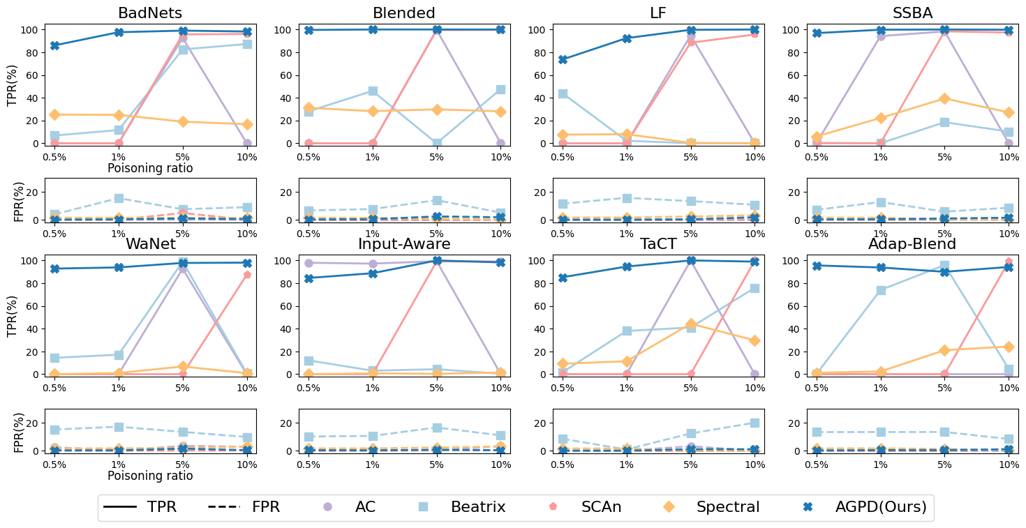
Figure 3: Detection of AGPD and compared detection methods with various poisoning ratios ranging from 0.5% to 10%.

4.3 Analysis

Difference between Activation and Activation Gradient.

In order to discern the distinctions between activations and activation gradients, we illustrate the distribution of the cosine similarity about activations and activation gradients across multiple convolutional layers in  Fig. 4. The visual analysis highlights that, despite the differentiation of activations in poisoned and clean samples being small, the differentiation becomes evident through activation gradients.

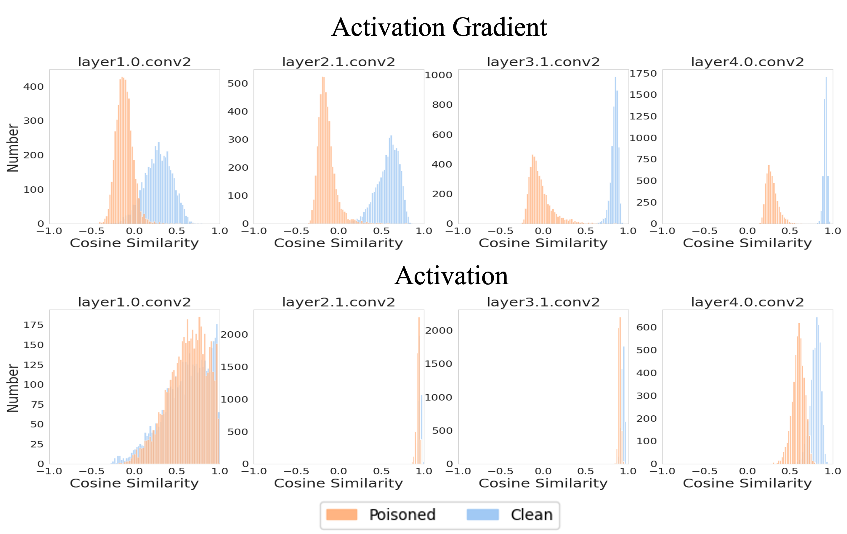
Figure 4: The visualization of the cosine similarity for the target class samples with the clean basis in multiple convolutional layers from the perspectives of activation gradient and feature.

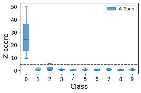
(a) The Z-score of CVBT for different labels in all-to-one attacks. 0 is the target label.

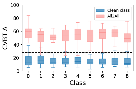
(b) The CVBT metric $\Delta$ of different labels in all-to-one and all-to-all attacks.

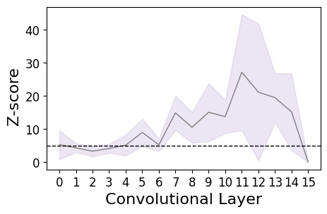
(c) The Z-score of CVBT for different convolution layers on Preact-ResNet18.

Figure 5: The statistic result of CVBT and its Z-score in all classes of CIFAR-10 and convolutional layers in Preact-ResNet18.

Analysis of CVBT Metric.

We employ visualizations to assess the practicality of the CVBT metric across various scenarios. 1) For each class, we present the dispersion of the Z-score to CVBT, under diverse backdoor attacks in Fig. 5(a). Notably, the Z-score for the target label 0 deviates significantly from the threshold $p$. This observation indicates that the target class(es) identification module effectively identifies abnormal behavior associated with the target label under various backdoor attacks. 2) In the case of the all-to-all poisoning strategy, where each label is treated as the target label, the target class(es) identification module becomes ineffective. Nevertheless, a distinct performance contrast is evident for the poisoned classes and the clean classes, as illustrated in Fig. 5(b). The dotted line represents the threshold for target class(es) identification. 3) Additionally, we present the distribution of the Z-score of CVBT across different layers. The solid line represents the mean under various attacks, while the grey area signifies a one-standard deviation range. Notably, several convolutional layers exhibit large Z-score values.

Accuracy of Target Class Identification.

We compare the accuracy of target class identification of AGPD with other three detection methods which are Beatrix [22], SCAn [31], and NC [34]. To evaluate their performance, we trained 120 backdoor models on CIFAR-10. The attack methods contain 8 dirty-label backdoor attacks, where the poisoning ratio ranges from $10\%$ to $1\%$, and the target label is from 0 to 4. The results of detection accuracy are shown in  Fig. 6. Note that the accuracy of target class identification of AGPD is higher than the compared method under different poisoning ratios. Even though SCAn has a competitive performance with AGPD, the accuracy of SCAn is lower than 20% with 1% poisoning ratio.

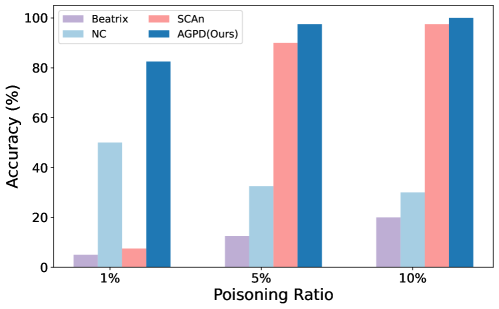
Figure 6: Accuracy of target label(s) recognition with three poisoning ratios on CIFAR10.

Effect of Number of Clean Samples.

In this part, we explore the influence of the size of the additional clean dataset on the detection performance of AGPD. Considering it could happen that the clean dataset’s distribution is inconsistent with the training dataset. Thus, we also assume the additional dataset collected by the defender is OOD. We collect the OOD dataset of CIFAR-10 from the first 10 classes of CIFAR-5m [24], and we extract 10 samples from each class. The additional clean dataset which is in distribution (ID) is collected from the validation dataset.  Fig. 7 shows the results of our method and SCAn [31] when the number of clean samples in each class is in the set $\{OOD,1,2,5,10\}$. It can be seen that AGPD exhibits significant advantages with an extremely limited number of samples, such as one sample per class or even OOD samples. When the number of clean samples in each class is one, the TPR values of AGPD on multiple attacks are above 90%, while also maintaining the FPR below 2%. Therefore, AGPD would be beneficial for saving time in practical applications, particularly in tasks involving hundreds of categories. However, for SCAn under OOD conditions, the TPR stands at merely about 10% across most attacks, TaCT [31] being the exception.

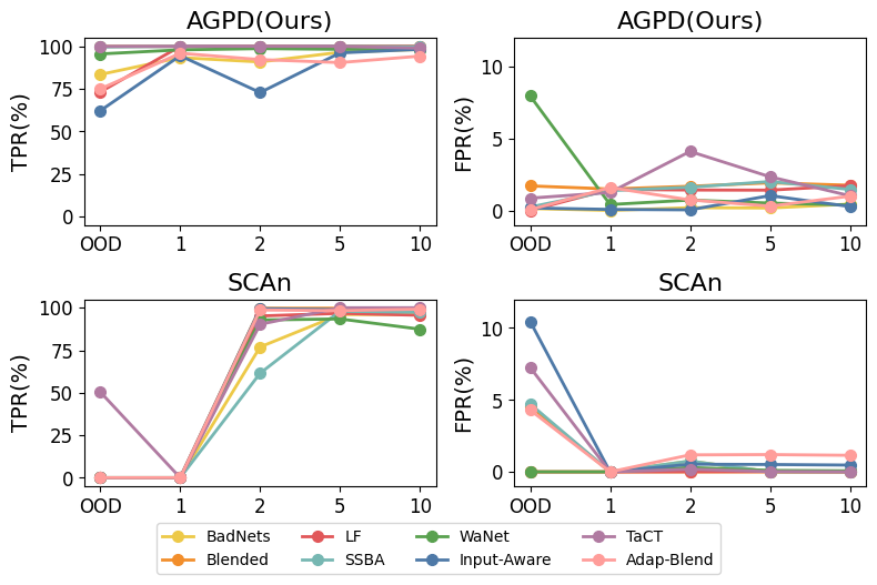
Figure 7: Detection effectiveness of AGPD and SCAn with the variance with the number of clean samples in each class. The situation that the collected clean samples are out of distribution has also been taken into account.

Supplementary Materials.

Due to the space limit, some additional materials are presented in Supplemenatry, including: (1) details of our method and experiments; (2) computational complexity of the proposed method; (3) evaluations in the multi-target, multi-trigger setting and different poisoning ratios on VGG19-BN; (4) sensitivity analysis to hyper-parameters $p,\tau,\xi$; (5) verification about the gradient circular dispersion (see Fig. 1) under various settings.

5 Conclusion

In conclusion, this paper presents Activation Gradient-based Poisoned Detection (AGPD), a novel method for detecting poisoned samples from an untrusted dataset. The key idea behind AGPD is to analyze the gradient with respect to activation, specifically the gradient circular distribution, of each sample to the backdoored model trained on the untrusted dataset. By designing a new metric called Cosine similarity Variation towards Basis Transition (CVBT), we demonstrate that the dispersion of the gradient circular distribution of the target class, which contains both poisoned and clean samples, is significantly higher compared to that of a clean class. This finding is consistent across various backdoor attacks, settings, and datasets. Based on this observation, a simple yet effective algorithm is proposed which involves identifying the target class(es) through outlier detection on CVBT scores and then progressively filtering out poisoned samples. Experimental results show that the proposed method can effectively filter out most poisoned samples while maintaining high accuracy on clean samples, demonstrating its robustness and effectiveness for poisoned sample detection. Overall, this paper contributes to the field of deep learning security by proposing a new perspective for analyzing poisoned samples and developing a reliable defense mechanism against data poisoning attacks.

Appendix A Summary

In the supplementary, we provide the details of the experimental setting of the backdoor attacks implemented and our method and in Sec. B. The complexity of the detection methods implemented is demonstrated in Sec. C. Besides, we complement the evaluations in the multi-target, multi-trigger setting and different poisoning ratios on VGG19-BN in Sec. D. In addition, we evaluate the sensitivity of our method on three hyper-parameters including $p$, $\tau$, and $\xi$ in Sec. E. The verification of the gradient circular dispersion of various backdoor attacks is shown in Sec. F. Furthermore, we present the detection results of AGPD and the comparison with other detectors on the GTSRB dataset in Sec. G.

Appendix B Experimental Details

In this section, we will introduce the experimental settings of backdoor attacks and our detection method on hyper-parameter settings. We will give more details about our detection method for all-to-all attacks in this part.

B.1 Backdoor Attacks

The hyper-parameters used in backdoor attacks are shown in Table 4. If the attack does not have any specific hyper-parameters, we will denote this with ‘/’. There are some common hyper-parameter configurations across these attack methods, such as training epoch, learning rate, and optimizer. In our experiment, we set the training epoch to 100 for CIFAR-10 and 200 for Tiny ImageNet. The learning rate scheduler is CosineAnnealingLR for CIFAR-10, and ReduceLROnPlateau for Tiny ImageNet. The learning rate of both of them is 0.01 and the optimizer is SGD. We show the poisoned samples of various backdoor attacks in Fig. 8.

Table 4: The hyper-parameters of implemented backdoor attacks for CIFAR-10.

	Category	Attack	Parameters	Usage	Value
All-to-one	non-clean label with sample-agnostic trigger	BadNets	/	/	/
		Blended	$\alpha$	the transparency of the trigger.	0.2
		LF	$\alpha$	fooling rate	0.2
	clean label with sample-agnostic trigger	SIG	$\Delta$	to generate sinusoidal signal.	40
			$f$		6
		LC	/	/	/
	non-clean label with sample-specific trigger	SSBA	/	/	/
		TaCT	$s-class$	the trigger will be added to samples in $s-class$ and change their labels to the target label.	a list
			$c-class$	samples in $c-class$ will only be added the trigger.	a list
			$c$	control the number of samples in $c-class$	0.1
		Adap-Blend	$m$	the probability of the area being masked.	0.5
	non-clean label with training control	WaNet	$s$	warping strength	0.5
			$k$	grid scale	4
			$\rho_{a}$	backdoor probability	=poisoning ratio
			$\rho_{n}$	the noise probability	0.1
		Input-Aware	$\lambda_{div}$	the diversity enforcement regularisation.	1
			$\rho_{b}$	the backdoor probability.	=poisoning ratio
			$\rho_{c}$	the cross-trigger probability.	0.1
All-to-all	non-clean label with sample-agnostic trigger	BadNets-A2A	$K$	to compute target labels.	10
	non-clean label with sample-specific trigger	SSBA-A2A
Multi-target Attack	non-clean label with sample-agnostic trigger	BadNets	$C$	to compute target labels	5
		Blended
		LF
	non-clean label with sample-specific trigger	SSBA
Multi-trigger Attack	non-clean label with sample-agnostic trigger	BadNets+Blended	$r_{1}$	the ratio of poisoned samples from BadNets.	0.05
		BadNets+LF
		BadNets+SSBA	$r_{2}$	the ratio of poisoned samples from another attack.	poisoning ratio-$r_{1}$

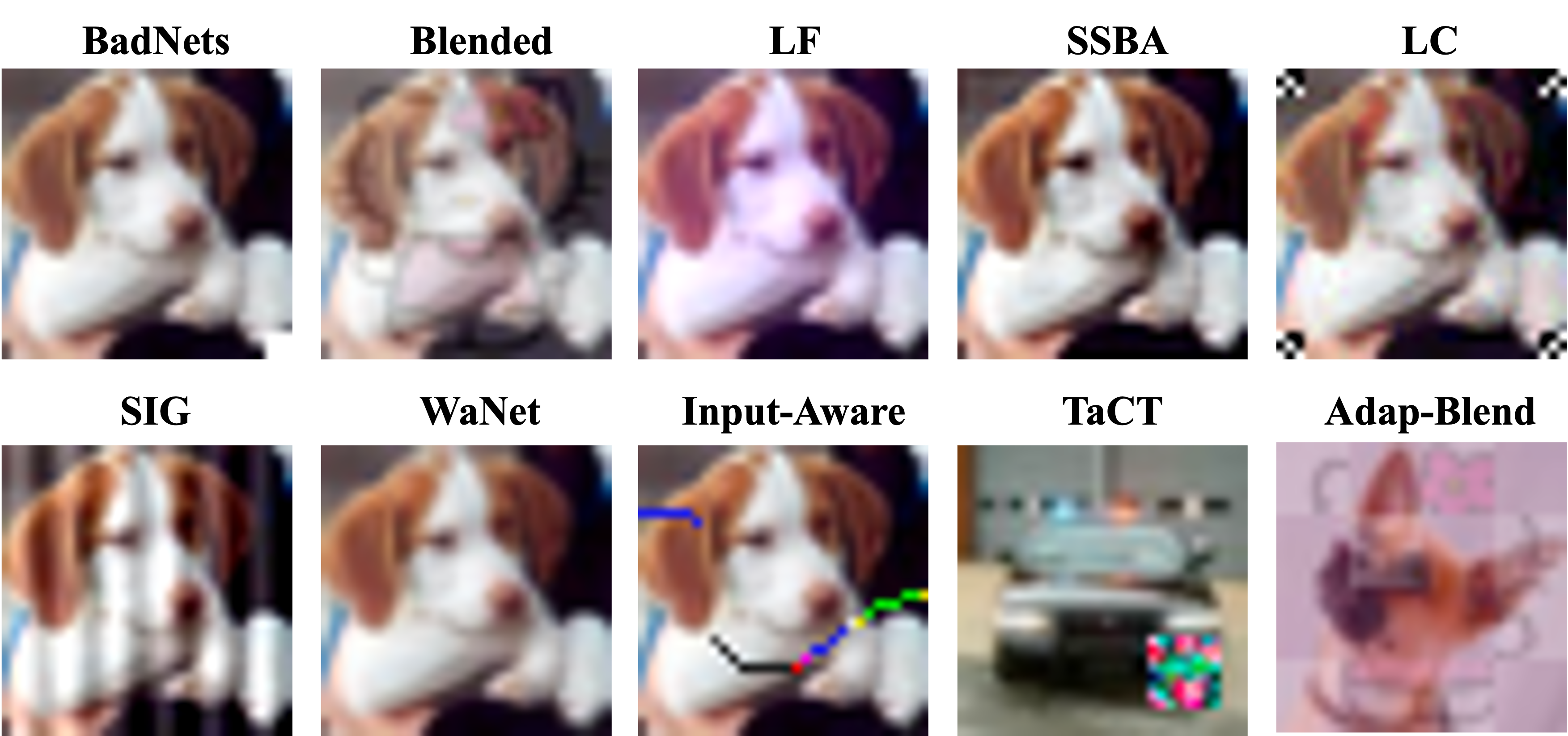
Figure 8: Examples of poisoned samples in various backdoor attacks.

B.2 Backdoor Detector: AGPD

The main text thoroughly explains the method by which AGPD identifies the target label and detects poisoned samples in various scenarios involving all-to-one, multi-target, and multi-trigger attacks. There are three hyper-parameters in AGPD, which are $\bm{p}$ (used in target class(es) identification), $\tau$, and $\xi$ (both of them are used in poisoned sample filtering). The values of these hyper-parameters are shown in Table. 6. In scenarios of all-to-all attacks, where each class is designated as a target, the Z-scores of CVBT are ineffective in distinctly identifying these target classes. This limitation may lead our method to erroneously presume that the dataset under examination is clean. To address this problem, if AGPD is unable to pinpoint any target label, we will examine the CVBT metrics $\Delta_{y}^{l}$ of all classes at layer $l$, ensuring a comprehensive assessment. The layer $l$ is chosen from the final four convolutional layers of the models. Specifically, we will calculate the CVBT metrics for each of the final four convolutional layers in the model. Any class whose CVBT metrics exceed the set threshold $\eta$ is marked as a target class. The layer $l$ that reveals the most target classes is then chosen. In our experiment, we set the threshold $\eta$ as 27.5 which has been added to Table 6. The threshold $\eta$ would be used in both all-to-all and multi-label attacks. In fact, the range for selecting $\eta$ is quite broad, as we have shown in Fig.8(b) in the main text.

Appendix C Complexity

We estimate the complexity of all detection methods by complexity analysis and recording their running time on poisoned sample detection. To ensure the accuracy of the running time of detection methods, we tested the average time of each detector on the CIFAR-10 datasets. We conduct eight backdoor attacks with 10% poisoning ratio. The results are displayed in Table 5.

Table 5: The time complexity of AGPD and the compared detection methods measured by complexity analysis and actual running time on CIFAR-10. The values in the brackets represent the standard deviations.

Detector	Complexity	Run time (minute)
AC	$O((F+D)N)$	1.02(0.01)
Beatrix	$O((D^{3}+F)N)$	8.92(0.38)
D-ST	$O(E(F+B+D)N)$	3.67(0.22)
FREAK	$O((F+B+C*H*W*log(H*W))N)$	0.94(0.02)
SCAn	$O((F+D)N)$	1.27(0.02)
Spectral	$O(NF+K(N/K)^{2}D)$	1.73(0.06)
STRIP	$O((N_{P}F+K)N)$	3.29( 0.02)
AGPD	$O((F+B+D)N)$	4.91(0.03)
General Settings	Epoch $E$; Samples $N$; Perturbation samples $N_{p}$;
	Feature Dimension $D$; Class $K$; Forward $F$; Backward $B$

Appendix D Evaluations on VGG19-BN

D.1 Multi-target and Multi-trigger

Table 6: The hyper-parameters for AGPD.

Hyper-Parameter	Usage	Value
$\bm{p}$	target class(es) identification.	5.2
$\tau$	poisoned sample filtering.	0.9
$\xi$		0.5
$\eta$	target class(es) identification.	27.5

Table 7: The detection of AGPD on multi-target and multi-trigger attacks on CIFAR-10 with VGG19-BN.

Type		Attack	STRIP			SCAn			AGPD (Ours)
			TPR$\uparrow$	FPR$\downarrow$	$F_{1}^{\omega}$$\uparrow$	TPR$\uparrow$	FPR$\downarrow$	$F_{1}^{\omega}$$\uparrow$	TPR$\uparrow$	FPR$\downarrow$	$F_{1}^{\omega}$$\uparrow$
Multi-target	Single trigger	BadNets	3.44	10.44	0.71	0.00	0.00	0.00	99.86	5.35	80.16
		Blended	0.34	11.06	0.07	0.00	0.00	0.00	100.00	8.24	72.95
		LF	6.36	9.99	1.35	0.00	0.00	0.00	79.92	3.70	42.76
		SSBA	38.68	15.07	10.11	0.00	0.00	0.00	99.92	5.47	80.01
	Multi-trigger	Blended+BadNets	61.14	6.17	23.18	88.70	0.01	63.54	95.14	5.59	66.91
		LF+BadNets	86.18	7.04	47.86	86.46	0.15	58.39	97.44	11.34	60.90
		SSBA+BadNets	37.46	9.73	10.33	84.06	0.10	53.79	92.26	3.56	64.44

The detection performance of AGPD against multi-target and multi-trigger attacks on VGG19-BN are shown in Table 7. AGPD achieved at least 79% TPR against multi-label single trigger attacks and arrived at 100% TPR against Blended. In the same attack scenarios, the TPR of compared detection methods doesn’t exceed 38.68%. Beside, in the multi-trigger attacks, the performance of AGPD is better than the compared methods. We can notice that the highest TPR is 97.44%.

D.2 Poisoning Ratios

We estimate the detection performance of AGPD against various backdoor attacks with different poisoning ratios and compare our method with four detectors. The model structure we utilized is VGG19-BN. The results are displayed in Fig. 9. It can be seen that our method achieves a higher TPR under most attacks compared to other methods, and our method is able to maintain relatively low FPR values.

Table 8: The detection performance of AGPD with the compared detectors on GTSRB using PreactResNet18.

Dataset	Attack	Backdoored	AC [21]			Beatrix [22]			D-ST [5]			FREAK [1]			SCAn [31]			Spectral [32]			STRIP [10]			AGPD (Ours)
		ACC/ASR	TPR$\uparrow$	FPR$\downarrow$	$F_{1}^{\omega}$$\uparrow$	TPR$\uparrow$	FPR$\downarrow$	$F_{1}^{\omega}$$\uparrow$	TPR$\uparrow$	FPR$\downarrow$	$F_{1}^{\omega}$$\uparrow$	TPR$\uparrow$	FPR$\downarrow$	$F_{1}^{\omega}$$\uparrow$	TPR$\uparrow$	FPR$\downarrow$	$F_{1}^{\omega}$$\uparrow$	TPR$\uparrow$	FPR$\downarrow$	$F_{1}^{\omega}$$\uparrow$	TPR$\uparrow$	FPR$\downarrow$	$F_{1}^{\omega}$$\uparrow$	TPR$\uparrow$	FPR$\downarrow$	$F_{1}^{\omega}$$\uparrow$
GTSRB	BadNets [12]	90.83/94.59	0.00	9.56	0.00	26.22	4.67	6.91	9.44	9.96	2.04	20.63	20.15	4.40	94.62	4.00	69.16	15.74	0.00	3.98	95.54	15.39	51.68	98.24	0.00	92.54
	Blended [6]	98.17/100.0	4.82	11.17	1.00	0.00	4.00	0.00	1.15	10.96	0.23	4.72	5.11	1.03	83.47	7.54	43.53	10.97	0.53	2.65	100.00	11.58	65.74	98.39	0.16	92.52
	LF [39]	97.97/99.58	0.18	7.05	0.04	0.00	3.62	0.00	0.18	11.32	0.04	14.82	14.52	3.20	96.40	6.24	68.54	10.86	0.54	2.62	99.90	14.50	60.33	97.04	0.00	87.94
	SSBA [18]	98.31/99.77	23.34	11.72	5.54	0.00	4.20	0.00	2.24	11.00	0.46	5.25	5.44	1.15	45.98	7.52	14.24	12.68	0.34	3.11	87.61	12.70	43.69	92.83	0.10	73.94
	WaNet [25]	97.05/96.16	0.00	7.59	0.00	1.01	6.42	0.21	8.76	10.00	1.87	14.91	14.97	3.17	60.83	0.00	25.65	10.72	0.52	2.58	7.83	14.34	1.59	98.75	0.16	93.90
	Input-Aware [26]	97.91/95.64	31.69	2.70	9.00	97.71	6.70	69.60	1.88	10.96	0.38	12.49	12.66	2.67	52.15	0.00	19.50	10.77	0.52	2.60	1.99	10.44	0.40	60.96	0.00	25.76
	TaCT [31]	98.78/99.91	0.00	8.39	0.00	97.50	8.70	65.92	1.68	11.10	0.34	6.25	6.66	1.36	59.03	2.70	23.10	15.82	0.00	4.01	0.15	15.17	0.03	65.69	0.33	29.64
	Adap-Blend [27]	97.66/80.42	0.00	9.34	0.00	11.48	11.92	2.48	2.53	10.84	0.52	11.33	10.65	2.47	50.74	3.95	17.48	12.02	0.41	2.93	20.48	12.40	4.72	96.56	0.09	85.87
	Average		7.50	8.44	1.95	29.24	6.28	18.14	3.48	10.77	0.73	11.30	11.27	2.43	67.90	3.99	35.15	12.45	0.36	3.06	51.69	13.31	28.52	88.56	0.11	72.76

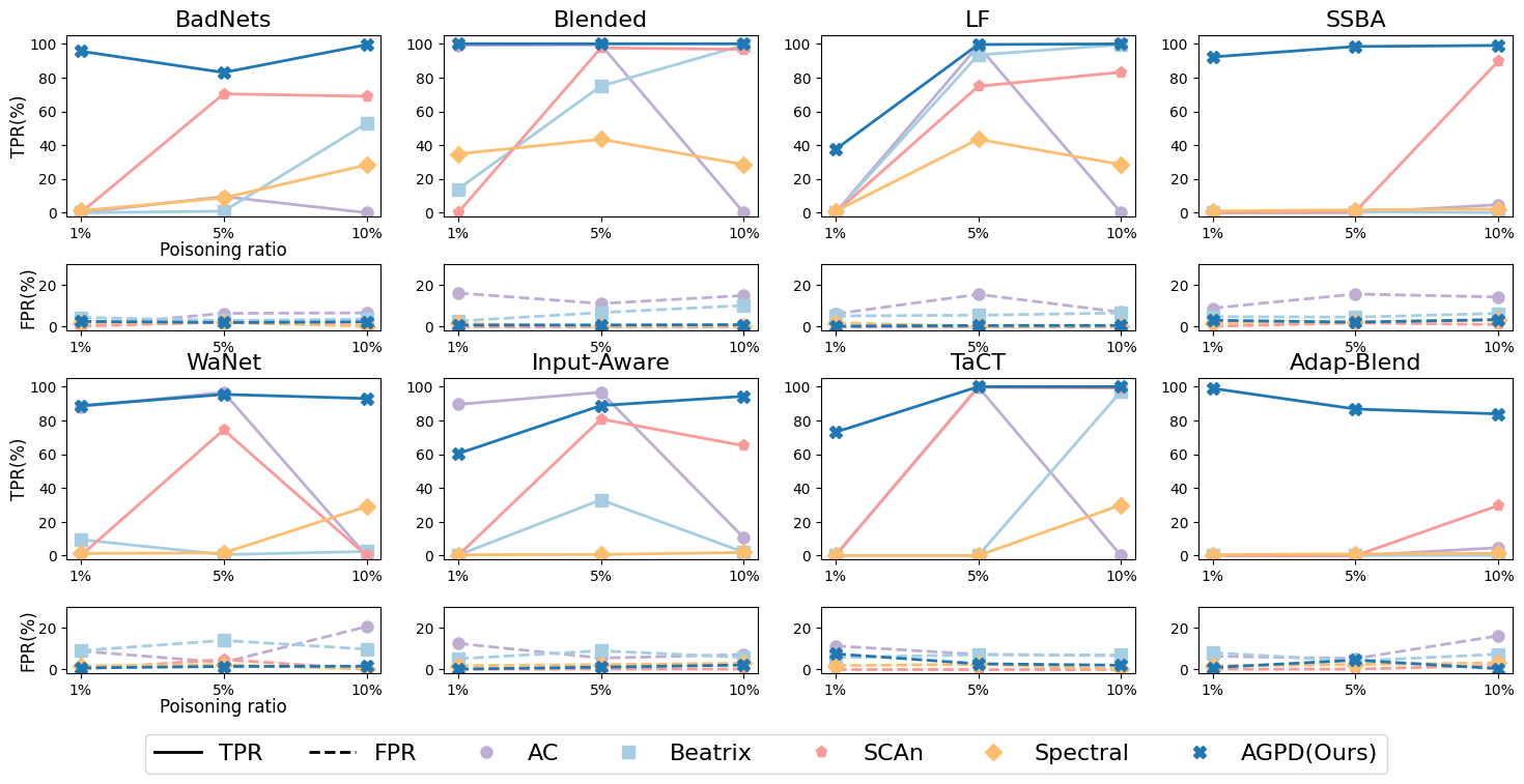
Figure 9: The detection performance of AGPD and the compared methods on VGG19-BN.

Appendix E Sensitivity of Hyper-parameters

To verify the sensitivity of AGPD against the variation of hyper-parameters, we assess the detection performance of our method under multiple hyper-parameter settings on Preact-ResNet18. The dataset we adopt here is CIFAR-10. For each set of hyper-parameters, we record the TPR, FPR, and weighted F1 score on 8 all-to-one backdoor attacks, including BadNets [12], Blended [6], SSBA [18], LF [39], WaNet [25], Input-Aware [26], TaCT [31], and Adap-Blend [27].

E.1 Threshold $p$

To evaluate the sensitivity of AGPD on the parameter $p$, we change the value of $p$ from 2.72 to 7.39, while keeping $\tau=0.9$ and $\xi=0.5$. The results of Preact-ResNet18 are exhibited in Fig. 10(a). It can be noticed that the mean of TPR is around 90% and infected slightly by the variation of hyper-parameter $p$. The variance of FPR gradually decreases with the increase of $p$, because the lower $p$ might misclassify some clean classes as target classes. The tendency of the curve of the weighted F1 score is similar to the TPR, which is nearly a straight line.

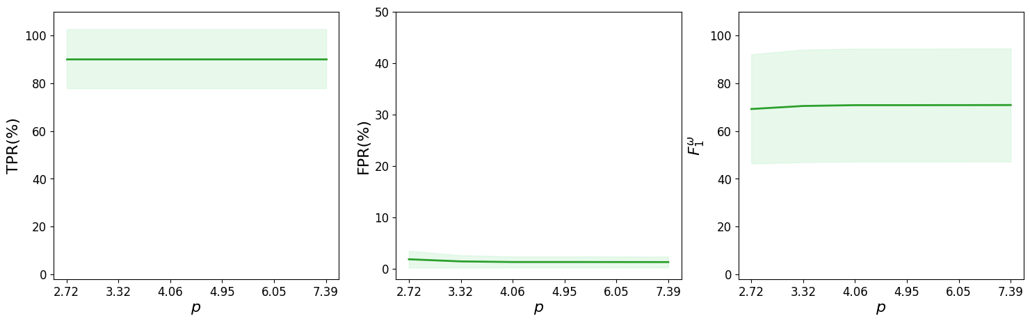
(a) Sensitivity on threshold $p$.

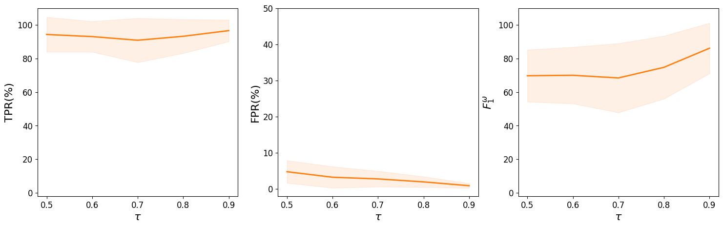
(b) Sensitivity on threshold $\tau$.

(c) Sensitivity on threshold $\xi$.

Figure 10: The detection performance of AGPD on Preact-ResNet18 with varying thresholds. The left is the mean-std (standard deviation) curve for TPR. The middle is the mean-std curve for FPR. The right is the mean-std curve for $F_{1}^{\omega}$.

E.2 Threshold $\tau$

To evaluate the sensitivity of AGPD on the parameter $\tau$, we fix $p=5.2$ and $\xi=0.5$ while changing the value of $\tau$ from 0.5 to 0.9. The results of Preact-ResNet18 are shown in Fig. 10(b). From Fig. 10(b), we find that the FPR decreases with the increase of $\tau$. In addition, the variance of TPR also decreases with the increase of $\tau$. Even though the ending condition of filtering is fixed to $\xi*\Delta_{y}^{l}$, a larger $\tau$ can avoid identifying clean samples as poisoned samples as much as possible.

E.3 Threshold $\xi$

The hyper-parameter $\xi$ is used to compute the ending condition of poisoned sample filtering. To verify the sensitivity of AGPD on the parameter $\xi$, we fix $p=5.2$ and $\tau=0.9$ while changing the value of $\xi$ from 0.3 to 0.8. We also test the detection performance of AGPD with the variation of $\xi$ on Preact-ResNet18. The results of these models are shown in Fig. 10(c). We discovered that the TPR of AGPD is close to 90% when $\xi$ is smaller than 0.5. However, if $\xi$ is larger than 0.5, the mean of TPR drops quickly and the variance of TPR also increases. This phenomenon indicates that there are many poisoned samples in the training dataset $\mathcal{D}_{bd}$. As for the mean curve of FPR, we noticed that the mean of FPR decreases with the increase of $\xi$, and the variance also reduces to 0. Therefore, a small $\xi$ will make more clean samples be filtered out, while a large $\xi$ will let more poisoned samples still stay in the dataset. Compared with the hyper-parameters $p$ and $\tau$, our method is more sensitive to the value $\xi$. An appropriate value $\xi$ plays an essential role in our method.

Appendix F GCDs for Various Attacks on CIFAR-10

We present the GCDs for all classes in CIFAR-10 in response to the backdoor attacks discussed in this paper, as shown in Fig. 11 and Fig. 12. These figures correspond to the model structures of Preact-ResNet18 and VGG19-BN, respectively. The target class is set to 0. It can be noticed that the target class (covering both black and blue arcs) occupies a longer arc on the circle compared with the clean classes across different model structures and backdoor attacks. Note that we moved all clean classes’ arcs to different areas on the circle to avoid visual overlap.

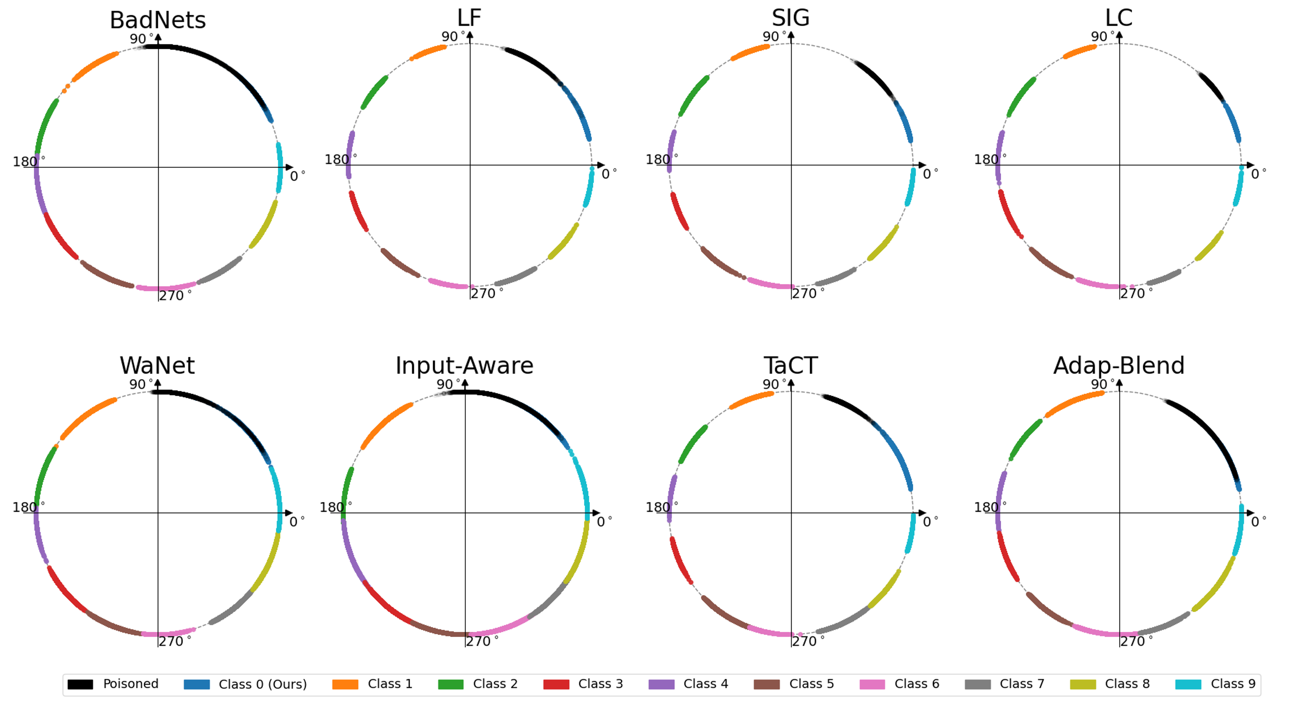
Figure 11: Gradient circular distributions (GCDs) of multiple backdoor attacks on CIFAR-10 with Preact-ResNet18.

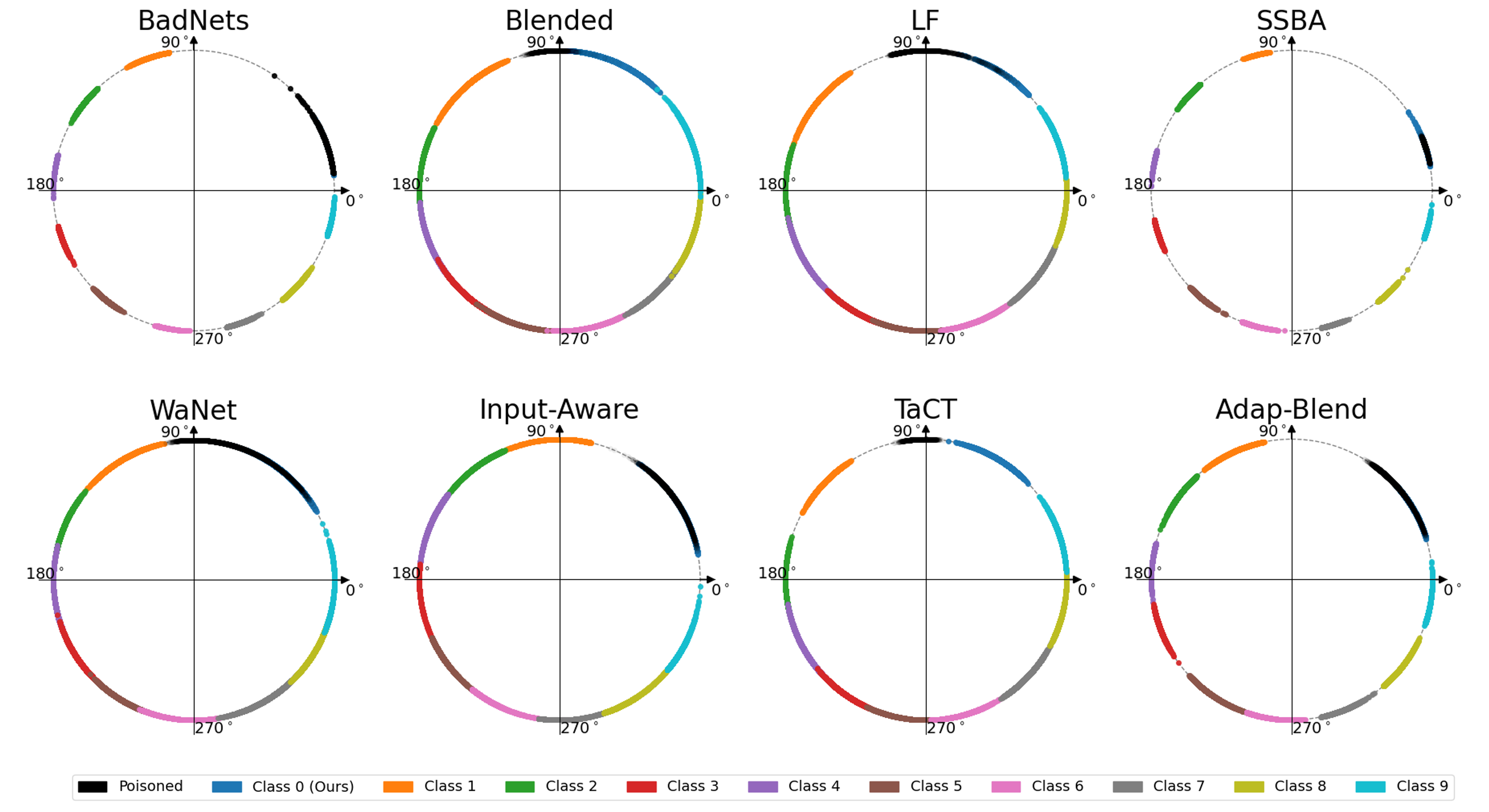
Figure 12: Gradient circular distributions (GCDs) of multiple backdoor attacks on CIFAR-10 with VGG19-BN.

Appendix G Evaluations of GTSRB

In the main text, it was noted that the datasets utilized comprise equal numbers of samples per class. For instance, each class in CIFAR-10 contains 5000 images, whereas Tiny ImageNet presents 500 samples per class. To enhance the comprehensiveness of our analysis, we included an evaluation of the GTSRB dataset in the supplementary. This particular dataset encompasses 43 distinct categories, with the sample count per category ranging from 200 to 2000. We compared AGPD with seven detection methods against eight backdoor attacks on this dataset with 10% poisoning ratio. The model structure we adopted is Preact-ResNet18 and the target class was designated as 0. In the experiment, the threshold $p$ is set to 4.06. It can be seen that AGPD attained an average TPR of 88.56%, higher than SCAn’s average TPR by 20.66%. Moreover, the average FPR is lower than SCAn’s by 3.88%. From the detection performances of the GTDRB dataset, it can be seen that AGPD is effective for detection tasks even when there is an imbalance in data volume among classes.

References

- Al Kader Hammoud et al. [2023] Hasan Abed Al Kader Hammoud, Adel Bibi, Philip HS Torr, and Bernard Ghanem. Don’t freak out: A frequency-inspired approach to detecting backdoor poisoned samples in dnns. In CVPR, pages 2337–2344, 2023.
- Barni et al. [2019a] Mauro Barni, Kassem Kallas, and Benedetta Tondi. A new backdoor attack in cnns by training set corruption without label poisoning. In ICIP, 2019a.
- Barni et al. [2019b] Mauro Barni, Kassem Kallas, and Benedetta Tondi. A new backdoor attack in cnns by training set corruption without label poisoning. In ICIP, pages 101–105. IEEE, 2019b.
- Chai and Chen [2022] Shuwen Chai and Jinghui Chen. One-shot neural backdoor erasing via adversarial weight masking. In NeurIPS, 2022.
- Chen et al. [2022] Weixin Chen, Baoyuan Wu, and Haoqian Wang. Effective backdoor defense by exploiting sensitivity of poisoned samples. In NeurIPS, 2022.
- Chen et al. [2017] Xinyun Chen, Chang Liu, Bo Li, Kimberly Lu, and Dawn Song. Targeted backdoor attacks on deep learning systems using data poisoning. arXiv preprint arXiv:1712.05526, 2017.
- Chou et al. [2020] Edward Chou, Florian Tramer, and Giancarlo Pellegrino. Sentinet: Detecting localized universal attacks against deep learning systems. In SPW, pages 48–54. IEEE, 2020.
- Doan et al. [2021] Khoa Doan, Yingjie Lao, Weijie Zhao, and Ping Li. Lira: Learnable, imperceptible and robust backdoor attacks. In ICCV, pages 11946–11956, 2021.
- Doan et al. [2022] Khoa D Doan, Yingjie Lao, and Ping Li. Marksman backdoor: Backdoor attacks with arbitrary target class. In NeurIPS, 2022.
- Gao et al. [2019] Yansong Gao, Change Xu, Derui Wang, Shiping Chen, Damith C Ranasinghe, and Surya Nepal. Strip: A defence against trojan attacks on deep neural networks. In ACSAC, pages 113–125, 2019.
- Gao et al. [2023] Yinghua Gao, Dongxian Wu, Jingfeng Zhang, Guanhao Gan, Shu-Tao Xia, Gang Niu, and Masashi Sugiyama. On the effectiveness of adversarial training against backdoor attacks. IEEE Transactions on Neural Networks and Learning Systems, 2023.
- Gu et al. [2019] Tianyu Gu, Kang Liu, Brendan Dolan-Gavitt, and Siddharth Garg. Badnets: Evaluating backdooring attacks on deep neural networks. IEEE Access, 7:47230–47244, 2019.
- He et al. [2016] Kaiming He, Xiangyu Zhang, Shaoqing Ren, and Jian Sun. Identity mappings in deep residual networks. In ECCV, pages 630–645. Springer, 2016.
- Huang et al. [2022] Kunzhe Huang, Yiming Li, Baoyuan Wu, Zhan Qin, and Kui Ren. Backdoor defense via decoupling the training process. In ICLR, 2022.
- Iglewicz and Hoaglin [1993] Boris Iglewicz and David C Hoaglin. Volume 16: how to detect and handle outliers. Quality Press, 1993.
- Krizhevsky et al. [2009] Alex Krizhevsky, Geoffrey Hinton, et al. Learning multiple layers of features from tiny images. 2009.
- Le and Yang [2015] Ya Le and Xuan Yang. Tiny imagenet visual recognition challenge. CS 231N, 7(7):3, 2015.
- Li et al. [2021a] Yuezun Li, Yiming Li, Baoyuan Wu, Longkang Li, Ran He, and Siwei Lyu. Invisible backdoor attack with sample-specific triggers. In ICCV, pages 16463–16472, 2021a.
- Li et al. [2021b] Yige Li, Xixiang Lyu, Nodens Koren, Lingjuan Lyu, Bo Li, and Xingjun Ma. Anti-backdoor learning: Training clean models on poisoned data. In NeurIPS, 2021b.
- Liu et al. [2018] Kang Liu, Brendan Dolan-Gavitt, and Siddharth Garg. Fine-pruning: Defending against backdooring attacks on deep neural networks. In RAID, pages 273–294. Springer, 2018.
- Ma et al. [2023a] Wanlun Ma, Derui Wang, Ruoxi Sun, Minhui Xue, Sheng Wen, and Yang Xiang. Detecting backdoor attacks on deep neural networks by activation clustering. In NDSS Symposium, 2023a.
- Ma et al. [2023b] Wanlun Ma, Derui Wang, Ruoxi Sun, Minhui Xue, Sheng Wen, and Yang Xiang. The ”beatrix” resurrections: Robust backdoor detection via gram matrices. In NDSS 2023, 2023b.
- Mu et al. [2023] Bingxu Mu, Zhenxing Niu, Le Wang, Xue Wang, Qiguang Miao, Rong Jin, and Gang Hua. Progressive backdoor erasing via connecting backdoor and adversarial attacks. In CVPR, pages 20495–20503, 2023.
- Nakkiran et al. [2020] Preetum Nakkiran, Behnam Neyshabur, and Hanie Sedghi. The deep bootstrap framework: Good online learners are good offline generalizers. arXiv preprint arXiv:2010.08127, 2020.
- Nguyen and Tran [2021] Anh Nguyen and Anh Tran. Wanet–imperceptible warping-based backdoor attack. arXiv preprint arXiv:2102.10369, 2021.
- Nguyen and Tran [2020] Tuan Anh Nguyen and Anh Tran. Input-aware dynamic backdoor attack. In NeurIPS, pages 3454–3464, 2020.
- Qi et al. [2023] Xiangyu Qi, Tinghao Xie, Yiming Li, Saeed Mahloujifar, and Prateek Mittal. Revisiting the assumption of latent separability for backdoor defenses. In ICLR, 2023.
- Salem et al. [2022] Ahmed Salem, Rui Wen, Michael Backes, Shiqing Ma, and Yang Zhang. Dynamic backdoor attacks against machine learning models. In S&P, pages 703–718, 2022.
- Simonyan and Zisserman [2014] Karen Simonyan and Andrew Zisserman. Very deep convolutional networks for large-scale image recognition. arXiv preprint arXiv:1409.1556, 2014.
- Souri et al. [2022] Hossein Souri, Liam Fowl, Rama Chellappa, Micah Goldblum, and Tom Goldstein. Sleeper agent: Scalable hidden trigger backdoors for neural networks trained from scratch. In NeurIPS, pages 19165–19178, 2022.
- Tang et al. [2021] Di Tang, XiaoFeng Wang, Haixu Tang, and Kehuan Zhang. Demon in the variant: Statistical analysis of DNNs for robust backdoor contamination detection. In USENIX Security, pages 1541–1558, 2021.
- Tran et al. [2018] Brandon Tran, Jerry Li, and Aleksander Madry. Spectral signatures in backdoor attacks. In NeurIPS, 2018.
- Turner et al. [2019] Alexander Turner, Dimitris Tsipras, and Aleksander Madry. Label-consistent backdoor attacks. arXiv preprint arXiv:1912.02771, 2019.
- Wang et al. [2019] Bolun Wang, Yuanshun Yao, Shawn Shan, Huiying Li, Bimal Viswanath, Haitao Zheng, and Ben Y Zhao. Neural cleanse: Identifying and mitigating backdoor attacks in neural networks. In S&P, pages 707–723. IEEE, 2019.
- Wei et al. [2023] Shaokui Wei, Mingda Zhang, Hongyuan Zha, and Baoyuan Wu. Shared adversarial unlearning: Backdoor mitigation by unlearning shared adversarial examples. In NeurIPS, 2023.
- Wu et al. [2022] Baoyuan Wu, Hongrui Chen, Mingda Zhang, Zihao Zhu, Shaokui Wei, Danni Yuan, and Chao Shen. Backdoorbench: A comprehensive benchmark of backdoor learning. In NeurIPS, pages 10546–10559, 2022.
- Wu et al. [2023] Baoyuan Wu, Li Liu, Zihao Zhu, Qingshan Liu, Zhaofeng He, and Siwei Lyu. Adversarial machine learning: A systematic survey of backdoor attack, weight attack and adversarial example. arXiv preprint arXiv:2302.09457, 2023.
- Wu and Wang [2021] Dongxian Wu and Yisen Wang. Adversarial neuron pruning purifies backdoored deep models. In NeurIPS, pages 16913–16925, 2021.
- Zeng et al. [2021] Yi Zeng, Won Park, Z Morley Mao, and Ruoxi Jia. Rethinking the backdoor attacks’ triggers: A frequency perspective. In ICCV, pages 16473–16481, 2021.
- Zeng et al. [2022] Yi Zeng, Si Chen, Won Park, Zhuoqing Mao, Ming Jin, and Ruoxi Jia. Adversarial unlearning of backdoors via implicit hypergradient. In ICLR. OpenReview.net, 2022.
- Zhang et al. [2022] Jie Zhang, Chen Dongdong, Qidong Huang, Jing Liao, Weiming Zhang, Huamin Feng, Gang Hua, and Nenghai Yu. Poison ink: Robust and invisible backdoor attack. IEEE Transactions on Image Processing, 31:5691–5705, 2022.
- Zheng et al. [2022a] Runkai Zheng, Rongjun Tang, Jianze Li, and Li Liu. Data-free backdoor removal based on channel lipschitzness. In ECCV, pages 175–191. Springer, 2022a.
- Zheng et al. [2022b] Runkai Zheng, Rongjun Tang, Jianze Li, and Li Liu. Pre-activation distributions expose backdoor neurons. In NeurIPS, 2022b.
- Zhu et al. [2023a] Mingli Zhu, Shaokui Wei, Li Shen, Yanbo Fan, and Baoyuan Wu. Enhancing fine-tuning based backdoor defense with sharpness-aware minimization. In ICCV, 2023a.
- Zhu et al. [2023b] Mingli Zhu, Shaokui Wei, Hongyuan Zha, and Baoyuan Wu. Neural polarizer: A lightweight and effective backdoor defense via purifying poisoned features. In NeurIPS, 2023b.