CSOT: Curriculum and Structure-Aware Optimal Transport for Learning with Noisy Labels

Abstract

Learning with noisy labels (LNL) poses a significant challenge in training a well-generalized model while avoiding overfitting to corrupted labels. Recent advances have achieved impressive performance by identifying clean labels and correcting corrupted labels for training. However, the current approaches rely heavily on the model’s predictions and evaluate each sample independently without considering either the global or local structure of the sample distribution. These limitations typically result in a suboptimal solution for the identification and correction processes, which eventually leads to models overfitting to incorrect labels. In this paper, we propose a novel optimal transport (OT) formulation, called Curriculum and Structure-aware Optimal Transport (CSOT). CSOT concurrently considers the inter- and intra-distribution structure of the samples to construct a robust denoising and relabeling allocator. During the training process, the allocator incrementally assigns reliable labels to a fraction of the samples with the highest confidence. These labels have both global discriminability and local coherence. Notably, CSOT is a new OT formulation with a nonconvex objective function and curriculum constraints, so it is not directly compatible with classical OT solvers. Here, we develop a lightspeed computational method that involves a scaling iteration within a generalized conditional gradient framework to solve CSOT efficiently. Extensive experiments demonstrate the superiority of our method over the current state-of-the-arts in LNL. Code is available at https://github.com/changwxx/CSOT-for-LNL.

1 Introduction

Deep neural networks (DNNs) have significantly boosted performance in various computer vision tasks, including image classification [33], object detection [61], and semantic segmentation [32]. However, the remarkable performance of deep learning algorithms heavily relies on large-scale high-quality human annotations, which are extremely expensive and time-consuming to obtain. Alternatively, mining large-scale labeled data based on a web search and user tags [49, 37] can provide a cost-effective way to collect labels, but this approach inevitably introduces noisy labels. Since DNNs can so easily overfit to noisy labels [4, 79], such label noise can significantly degrade performance, giving rise to a challenging task: learning with noisy labels (LNL) [50, 52, 46].

Numerous strategies have been proposed to mitigate the negative impact of noisy labels, including loss correction based on transition matrix estimation [35], re-weighting [60], label correction [76] and sample selection [52]. Recent advances have achieved impressive performance by identifying clean labels and correcting corrupted labels for training. However, current approaches rely heavily on the model’s predictions to identify or correct labels even if the model is not yet sufficiently trained. Moreover, these approaches often evaluate each sample independently, disregarding the global or local structure of the sample distribution. Hence, the identification and correction process results in a suboptimal solution which eventually leads to a model overfitting to incorrect labels.

In light of the limitations of distribution modeling, optimal transport (OT) offers a promising solution by optimizing the global distribution matching problem that searches for an efficient transport plan from one distribution to another. To date, OT has been applied in various machine learning tasks [11, 83, 28]. In particular, OT-based pseudo-labeling [11, 73] attempts to map samples to class centroids, while considering the inter-distribution matching of samples and classes. However, such an approach could also produce assignments that overlook the inherent coherence structure of the sample distribution, i.e. intra-distribution coherence. More specifically, the cost matrix in OT relies on pairwise metrics, so two nearby samples could be mapped to two far-away class centroids (Fig. 1).

In this paper, to enhance intra-distribution coherence, we propose a new OT formulation for denoising and relabeling, called Structure-aware Optimal Transport (SOT). This formulation fully considers the intra-distribution structure of the samples and produces robust assignments with both global discriminability and local coherence. Technically speaking, we introduce local coherent regularized terms to encourage both prediction- and label-level local consistency in the assignments. Furthermore, to avoid generating incorrect labels in the early stages of training or cases with high noise ratios, we devise Curriculum and Structure-aware Optimal Transport (CSOT) based on SOT. CSOT constructs a robust denoising and relabeling allocator by relaxing one of the equality constraints to allow only a fraction of the samples with the highest confidence to be selected. These samples are then assigned with reliable pseudo labels. The allocator progressively selects and relabels batches of high-confidence samples based on an increasing budget factor that controls the number of selected samples. Notably, CSOT is a new OT formulation with a nonconvex objective function and curriculum constraints, so it is significantly different from the classical OT formulations. Hence, to solve CSOT efficiently, we developed a lightspeed computational method that involves a scaling iteration within a generalized conditional gradient framework [59].

Our contribution can be summarized as follows: 1) We tackle the denoising and relabeling problem in LNL from a new perspective, i.e. simultaneously considering the inter- and intra-distribution structure for generating superior pseudo labels using optimal transport. 2) To fully consider the intrinsic coherence structure of sample distribution, we propose a novel optimal transport formulation, namely Curriculum and Structure-aware Optimal Transport (CSOT), which constructs a robust denoising and relabeling allocator that mitigates error accumulation. This allocator selects a fraction of high-confidence samples, which are then assigned reliable labels with both global discriminability and local coherence. 3) We further develop a lightspeed computational method that involves a scaling iteration within a generalized conditional gradient framework to efficiently solve CSOT. 4) Extensive experiments demonstrate the superiority of our method over state-of-the-art methods in LNL.

2 Related Work

Learning with noisy labels.

LNL is a well-studied field with numerous strategies having been proposed to solve this challenging problem, such as robust loss design [82, 70], loss correction [35, 56], loss re-weighting [60, 80] and sample selection [52, 31, 41]. Currently, the methods that are delivering superior performance mainly involve learning from both selected clean labels and relabeled corrupted labels [46, 45]. The mainstream approaches for identifying clean labels typically rely on the small-loss criterion [31, 77, 71, 14]. These methods often model per-sample loss distributions using a Beta Mixture Model [51] or a Gaussian Mixture Model [57], treating samples with smaller loss as clean ones [3, 71, 46]. The label correction methods, such as PENCIL [76], Selfie [63], ELR [50], and DivideMix [46], typically adopt a pseudo-labeling strategy that leverages the DNN’s predictions to correct the labels. However, these approaches evaluate each sample independently without considering the correlations among samples, which leads to a suboptimal identification and correction solution. To this end, some work [55, 45] attempt to leverage $k$-nearest neighbor predictions [6] for clean identification and label correction. Besides, to further select and correct noisy labels robustly, OT Cleaner [73], as well as concurrent OT-Filter [23], designed to consider the global sample distribution by formulating pseudo-labeling as an optimal transport problem. In this paper, we propose CSOT to construct a robust denoising and relabeling allocator that simultaneously considers both the global and local structure of sample distribution so as to generate better pseudo labels.

Optimal transport-based pseudo-labeling.

OT is a constrained optimization problem that aims to find the optimal coupling matrix to map one probability distribution to another while minimizing the total cost [40]. OT has been formulated as a pseudo-labeling (PL) technique for a range of machine learning tasks, including class-imbalanced learning [44, 28, 68], semi-supervised learning [65, 54, 44], clustering [5, 11, 25], domain adaptation [83, 12], label refinery [83, 68, 73, 23], and others. Unlike prediction-based PL [62], OT-based PL optimizes the mapping samples to class centroids, while considering the global structure of the sample distribution in terms of marginal constraints instead of per-sample predictions. For example, Self-labelling [5] and SwAV [11], which are designed for self-supervised learning, both seek an optimal equal-partition clustering to avoid the model’s collapse. In addition, because OT-based PL considers marginal constraints, it can also consider class distribution to solve class-imbalance problems [44, 28, 68]. However, these approaches only consider the inter-distribution matching of samples and classes but do not consider the intra-distribution coherence structure of samples. By contrast, our proposed CSOT considers both the inter- and intra-distribution structure and generates superior pseudo labels for noise-robust learning.

Curriculum learning.

Curriculum learning (CL) attempts to gradually increase the difficulty of the training samples, allowing the model to learn progressively from easier concepts to more complex ones [42]. CL has been applied to various machine learning tasks, including image classification [38, 84], and reinforcement learning [53, 2]. Recently, the combination of curriculum learning and pseudo-labeling has become popular in semi-supervised learning. These methods mainly focus on dynamic confident thresholding [69, 29, 75] instead of adopting a fixed threshold [62]. Flexmatch [78] designs class-wise thresholds and lowers the thresholds for classes that are more difficult to learn. Different from dynamic thresholding approaches, SLA [65] only assigns pseudo labels to easy samples gradually based on an OT-like problem. In the context of LNL, CurriculumNet [30] designs a curriculum by ranking the complexity of the data using its distribution density in a feature space. Alternatively, RoCL [85] selects easier samples considering both the dynamics of the per-sample loss and the output consistency. Our proposed CSOT constructs a robust denoising and relabeling allocator that gradually assigns high-quality labels to a fraction of the samples with the highest confidence. This encourages both global discriminability and local coherence in assignments.

3 Preliminaries

Optimal transport.

Here we briefly recap the well-known formulation of OT. Given two probability simplex vectors $\bm{\alpha}$ and $\bm{\beta}$ indicating two distributions, as well as a cost matrix $\mathbf{C}\in\mathbb{R}^{|\bm{\alpha}|\times|\bm{\beta}|}$, where $|\bm{\alpha}|$ denotes the dimension of $\bm{\alpha}$, OT aims to seek the optimal coupling matrix $\mathbf{Q}$ by minimizing the following objective

$$\min_{\mathbf{Q}\in\mathbf{\Pi}(\bm{\alpha},\bm{\beta})}\left<\mathbf{C},\mathbf{Q}\right>,$$ (1)

where $\left<\cdot,\cdot\right>$ denote Frobenius dot-product. The coupling matrix $\mathbf{Q}$ satisfies the polytope $\mathbf{\Pi}(\bm{\alpha},\bm{\beta})=\left\{\mathbf{Q}\in\mathbb{R}_{+}^{|\bm{\alpha}|\times|\bm{\beta}|}|\mathbf{Q}\mathds{1}_{|\bm{\beta}|}=\bm{\alpha},\;\mathbf{Q}^{\top}\mathds{1}_{|\bm{\alpha}|}=\bm{\beta}\right\}$, where $\bm{\alpha}$ and $\bm{\beta}$ are essentially marginal probability vectors. Intuitively speaking, these two marginal probability vectors can be interpreted as coupling budgets, which control the mapping intensity of each row and column in $\mathbf{Q}$.

Pseudo-labeling based on optimal transport.

Let $\mathbf{P}\in\mathbb{R}_{+}^{B\times C}$ denote classifier softmax predictions, where $B$ is the batch size of samples, and $C$ is the number of classes. The OT-based PL considers mapping samples to class centroids and the cost matrix $\mathbf{C}$ can be formulated as $-\log\mathbf{P}$ [65, 68]. We can rewrite the objective for OT-based PL based on Problem (1) as follows

$$\min_{\mathbf{Q}\in\mathbf{\Pi}(\frac{1}{B}\mathds{1}_{B},\frac{1}{C}\mathds{1}_{C})}\left<-\log\mathbf{P},\mathbf{Q}\right>,$$ (2)

where $\mathds{1}_{d}$ indicates a $d$-dimensional vector of ones. The pseudo-labeling matrix can be obtained by normalization: $B\mathbf{Q}$. Unlike prediction-based PL [62] which evaluates each sample independently, OT-based PL considers inter-distribution matching of samples and classes, as well as the global structure of sample distribution, thanks to the equality constraints.

Sinkhorn algorithm for classical optimal transport problem.

Directly optimizing the exact OT problem would be time-consuming, and an entropic regularization term is introduced [19]: $\min_{\mathbf{Q}\in\mathbf{\Pi}(\bm{\alpha},\bm{\beta})}\left<\mathbf{C},\mathbf{Q}\right>+\varepsilon\left<\mathbf{Q},\log\mathbf{Q}\right>$ , where $\varepsilon>0$. The entropic regularization term enables OT to be approximated efficiently by the Sinkhorn algorithm [19], which involves matrix scaling iterations executed efficiently by matrix multiplication on GPU.

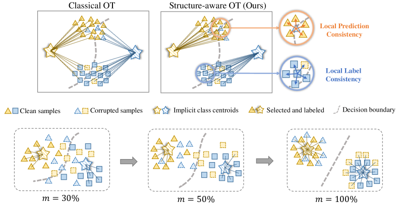
Figure 1: (Top) Comparison between classical OT and our proposed Structure-aware OT. Classical OT tends to mismatch two nearby samples to two far-away class centroids when the decision boundary is not accurate enough. To mitigate this, our SOT generates local consensus assignments for each sample by preserving prediction-level and label-level consistency. Notably, for vague samples located near the ambiguous decision boundary, SOT rectifies their assignments based on the neighborhood majority consistency. (Bottom) The illustration of our curriculum denoising and relabeling based on proposed CSOT. The decision boundary refers to the surface that separates two classes by the classifier. The $m$ represents the curriculum budget that controls the number of selected samples and progressively increases during the training process.

4 Methodology

Problem setup.

Let $\mathcal{D}_{train}=\{(\mathbf{x}_{i},y_{i})\}_{i=1}^{N}$ denote the noisy training set, where $\mathbf{x}_{i}$ is an image with its associated label $y_{i}$ over $C$ classes, but whether the given label is accurate or not is unknown. We call the correctly-labeled ones as clean, and the mislabeled ones as corrupted. LNL aims to train a network that is robust to corrupted labels and achieves high accuracy on a clean test set.

4.1 Structure-Aware Optimal Transport for Denoising and Relabeling

Even though existing OT-based PL considers the global structure of sample distribution, the intrinsic coherence structure of the samples is ignored. Specifically, the cost matrix in OT relies on pairwise metrics and thus two nearby samples could be mapped to two far-away class centroids. To further consider the intrinsic coherence structure, we propose a Structure-aware Optimal Transport (SOT) for denoising and relabeling, which promotes local consensus assignment by encouraging prediction-level and label-level consistency, as shown in Fig. 1.

Our proposed SOT for denoising and relabeling is formulated by adding two local coherent regularized terms based on Problem (2). Given a cosine similarity $\mathbf{S}\in\mathbb{R}^{B\times B}$ among samples in feature space, a one-hot label matrix $\mathbf{L}\in\mathbb{R}^{B\times C}$ transformed from given noisy labels, and a softmax prediction matrix $\mathbf{P}\in\mathbb{R}_{+}^{B\times C}$, SOT is formulated as follows

$$\min_{\mathbf{Q}\in\mathbf{\Pi}(\frac{1}{B}\mathds{1}_{B},\frac{1}{C}\mathds{1}_{C})}\left<-\log\mathbf{P},\mathbf{Q}\right>+\kappa\left(\Omega^{\mathbf{P}}(\mathbf{Q})+\Omega^{\mathbf{L}}(\mathbf{Q})\right),$$ (3)

where the local coherent regularized terms $\Omega^{\mathbf{P}}$ and $\Omega^{\mathbf{L}}$ encourages prediction-level and label-level local consistency respectively, and are defined as follows

$$\Omega^{\mathbf{P}}(\mathbf{Q})=-\sum_{i,j}\mathbf{S}_{ij}\sum_{k}\mathbf{P}_{ik}\mathbf{P}_{jk}\mathbf{Q}_{ik}\mathbf{Q}_{jk}=-\left<\mathbf{S},\left(\mathbf{P}\odot\mathbf{Q}\right)\left(\mathbf{P}\odot\mathbf{Q}\right)^{\top}\right>,$$ (4)

$$\Omega^{\mathbf{L}}(\mathbf{Q})=-\sum_{i,j}\mathbf{S}_{ij}\sum_{k}\mathbf{L}_{ik}\mathbf{L}_{jk}\mathbf{Q}_{ik}\mathbf{Q}_{jk}=-\left<\mathbf{S},\left(\mathbf{L}\odot\mathbf{Q}\right)\left(\mathbf{L}\odot\mathbf{Q}\right)^{\top}\right>,$$ (5)

where $\odot$ indicates element-wise multiplication. To be more specific, $\Omega^{\mathbf{P}}$ encourages assigning larger weight to $\mathbf{Q}_{ik}$ and $\mathbf{Q}_{jk}$ if the $i$-th sample is very close to the $j$-th sample, and their predictions $\mathbf{P}_{ik}$ and $\mathbf{P}_{jk}$ from the $k$-th class centroid are simultaneously high. Analogously, $\Omega^{\mathbf{L}}$ encourages assigning larger weight to those samples whose neighborhood label consistency is rather high. Unlike the formulation proposed in [1, 16], which focuses on sample-to-sample mapping, our method introduces a sample-to-class mapping that leverages the intrinsic coherence structure within the samples.

4.2 Curriculum and Structure-Aware Optimal Transport for Denoising and Relabeling

In the early stages of training or in scenarios with a high noise ratio, the predictions and feature representation would be vague and thus lead to the wrong assignments for SOT. For the purpose of robust clean label identification and corrupted label correction, we further propose a Curriculum and Structure-aware Optimal Transport (CSOT), which constructs a robust curriculum allocator. This curriculum allocator gradually selects a fraction of the samples with high confidence from the noisy training set, controlled by a budget factor, then assigns reliable pseudo labels for them.

Our proposed CSOT for denoising and relabeling is formulated by introducing new curriculum constraints based on SOT in Problem (3). Given curriculum budget factor $m\in[0,1]$, our CSOT seeks optimal coupling matrix $\mathbf{Q}$ by minimizing following objective

$$\min_{\mathbf{Q}}\left<-\log\mathbf{P},\mathbf{Q}\right>+\kappa\left(\Omega^{\mathbf{P}}(\mathbf{Q})+\Omega^{\mathbf{L}}(\mathbf{Q})\right)$$ (6)

$$\text{s.t.}\quad\mathbf{Q}\in \left\{\mathbf{Q}\in\mathbb{R}_{+}^{B\times C}|\mathbf{Q}\mathds{1}_{C}\leq\frac{1}{B}\mathds{1}_{B},\mathbf{Q}^{\top}\mathds{1}_{B}=\frac{m}{C}\mathds{1}_{C}\right\}.$$

Unlike SOT, which enforces an equality constraint on the samples, CSOT relaxes this constraint and defines the total coupling budget as $m\in[0,1]$, where $m$ represents the expected total sum of $\mathbf{Q}$. Intuitively speaking, $m=0.5$ indicates that top $50\%$ confident samples are selected from all the classes, avoiding only selecting the same class for all the samples within a mini-batch. And the budget $m$ progressively increases during the training process, as shown in Fig. 1.

Based on the optimal coupling matrix $\mathbf{Q}$ solved from Problem (LABEL:eq:CSOT), we can obtain pseudo label by argmax operation, i.e. $\hat{y}_{i}=\operatorname*{argmax}_{j}\mathbf{Q}_{ij}$. In addition, we define the general confident scores of samples as $\mathcal{W}=\{w_{0},w_{1},\cdots,w_{B-1}\}$, where $w_{i}=\mathbf{Q}_{i\hat{y}_{i}}/(m/C)$. Since our curriculum allocator assigns weight to only a fraction of samples controlled by $m$, we use topK($\mathcal{S}$,$k$) operation (return top-$k$ indices of input set $\mathcal{S}$) to identify selected samples denoted as $\delta_{i}$

$$\delta_{i}=\left\{\begin{aligned} 1,&\quad i\in\texttt{topK}(\mathcal{W},\left\lfloor mB\right\rfloor)\\ 0,&\quad\text{otherwise}\end{aligned}\right.,$$ (7)

where $\left\lfloor\cdot\right\rfloor$ indicates the round down operator. Then the noisy dataset $\mathcal{D}_{train}$ can be splited into $\mathcal{D}_{clean}$ and $\mathcal{D}_{corrupted}$ as follows

$$\begin{aligned} \mathcal{D}_{clean}\leftarrow\left\{(\mathbf{x}_{i},y_{i},w_{i})|\hat{y}_{i}=y_{i},\delta_{i}=1,\forall(\mathbf{x}_{i},y_{i})\in\mathcal{D}_{train}\right\},\\ \mathcal{D}_{corrupted}\leftarrow\left\{(\mathbf{x}_{i},\hat{y}_{i},w_{i})|\hat{y}_{i}\neq y_{i},\forall(\mathbf{x}_{i},y_{i})\in\mathcal{D}_{train}\right\}.\end{aligned}$$ (8)

4.3 Training Objectives

To avoid error accumulation in the early stage of training, we adopt a two-stage training scheme. In the first stage, the model is supervised by progressively selected clean labels and self-supervised by unselected samples. In the second stage, the model is semi-supervised by all denoised labels. Notably, we construct our training objective mainly based on Mixup loss $\mathcal{L}^{mix}$ and Label consistency loss $\mathcal{L}^{lab}$ same as NCE [45], and a self-supervised loss $\mathcal{L}^{simsiam}$ proposed in SimSiam [15]. The detailed formulations of mentioned loss and training process are given in Appendix. Our two-stage training objective can be constructed as follows

$$\mathcal{L}^{sup}=\mathcal{L}^{mix}_{\mathcal{D}_{clean}}+\mathcal{L}^{lab}_{\mathcal{D}_{clean}}+\lambda_{1}\mathcal{L}^{simsiam}_{\mathcal{D}_{corrupted}},$$ (9)

$$\mathcal{L}^{semi}=\mathcal{L}^{mix}_{\mathcal{D}_{clean}}+\mathcal{L}^{lab}_{\mathcal{D}_{clean}}+\lambda_{2}\mathcal{L}^{lab}_{\mathcal{D}_{corrupted}}.$$ (10)

5 Lightspeed Computation for CSOT

The proposed CSOT is a new OT formulation with nonconvex objective function and curriculum constraints, which cannot be solved directly by classical OT solvers. To this end, we develop a lightspeed computational method that involves a scaling iteration within a generalized conditional gradient framework to solve CSOT efficiently. Specifically, we first introduce an efficient scaling iteration for solving the OT problem with curriculum constraints without considering the local coherent regularized terms, i.e. Curriculum OT (COT). Then, we extend our approach to solve the proposed CSOT problem, which involves a nonconvex objective function and curriculum constraints.

5.1 Solving Curriculum Optimal Transport

For convenience, we formulate curriculum constraints in Probelm (LABEL:eq:CSOT) in a more general form. Given two vectors $\bm{\alpha}$ and $\bm{\beta}$ that satisfy $\left\|\bm{\alpha}\right\|_{1}\geq\left\|\bm{\beta}\right\|_{1}=m$, a general polytope of curriculum constraints $\mathbf{\Pi}^{\text{c}}(\bm{\alpha},\bm{\beta})$ is formulated as

$$\mathbf{\Pi}^{\text{c}}(\bm{\alpha},\bm{\beta})=\left\{\mathbf{Q}\in\mathbb{R}_{+}^{|\bm{\alpha}|\times|\bm{\beta}|}|\mathbf{Q}\mathds{1}_{|\bm{\beta}|}\leq\bm{\alpha},\mathbf{Q}^{\top}\mathds{1}_{|\bm{\alpha}|}=\bm{\beta}\right\}.$$ (11)

For the efficient computation purpose, we consider an entropic regularized version of COT

$$\min_{\mathbf{Q}\in\mathbf{\Pi}^{\text{c}}(\bm{\alpha},\bm{\beta})}\left<\mathbf{C},\mathbf{Q}\right>+\varepsilon\left<\mathbf{Q},\log\mathbf{Q}\right>,$$ (12)

where we denote the cost matrix $\mathbf{C}:=-\log\mathbf{P}$ in Probelm (LABEL:eq:CSOT) for simplicity. Inspired by [8], Problem (12) can be easily re-written as the Kullback-Leibler (KL) projection: $\min_{\mathbf{Q}\in\mathbf{\Pi}^{\text{c}}(\bm{\alpha},\bm{\beta})}\varepsilon\text{KL}(\mathbf{Q}|e^{-\mathbf{C}/\varepsilon})$. Besides, the polytope $\mathbf{\Pi}^{\text{c}}(\bm{\alpha},\bm{\beta})$ can be expressed as an intersection of two convex but not affine sets, i.e.

$$\mathcal{C}_{1}\overset{\underset{\mathrm{def}}{}}{=}\left\{\mathbf{Q}\in\mathbb{R}_{+}^{|\bm{\alpha}|\times|\bm{\beta}|}|\mathbf{Q}\mathds{1}_{|\bm{\beta}|}\leq\bm{\alpha}\right\}\quad\text{and}\quad\mathcal{C}_{2}\overset{\underset{\mathrm{def}}{}}{=}\left\{\mathbf{Q}\in\mathbb{R}_{+}^{|\bm{\alpha}|\times|\bm{\beta}|}|\mathbf{Q}^{\top}\mathds{1}_{|\bm{\alpha}|}=\bm{\beta}\right\}.$$ (13)

In light of this, Problem (12) can be solved by performing iterative KL projection between $\mathcal{C}_{1}$ and $\mathcal{C}_{2}$, namely Dykstra’s algorithm [21] shown in Appendix.

Lemma 1.

(Efficient scaling iteration for Curriculum OT) When solving Problem (12) by iterating Dykstra’s algorithm, the matrix $\mathbf{Q}^{(n)}$ at $n$ iteration is a diagonal scaling of $\mathbf{K}:=e^{-\mathbf{C}/\varepsilon}$, which is the element-wise exponential matrix of $-\mathbf{C}/\varepsilon$:

$$\mathbf{Q}^{(n)}={\rm{diag}}\left(\bm{u}^{(n)}\right)\mathbf{K}{\rm{diag}}\left(\bm{v}^{(n)}\right),$$ (14)

where the vectors $\bm{u}^{(n)}\in\mathbb{R}^{|\bm{\alpha}|}$, $\bm{v}^{(n)}\in\mathbb{R}^{|\bm{\beta}|}$ satisfy $\bm{v}^{(0)}=\mathds{1}_{|\bm{\beta}|}$ and follow the recursion formula

$$\bm{u}^{(n)}=\min\left(\frac{\bm{\alpha}}{\mathbf{K}\bm{v}^{(n-1)}},\mathds{1}_{|\bm{\alpha}|}\right)\quad{\rm{and}}\quad\bm{v}^{(n)}=\frac{\bm{\beta}}{\mathbf{K}^{\top}\bm{u}^{(n)}}.$$ (15)

The proof is given in the Appendix. Lemma 1 allows a fast implementation of Dykstra’s algorithm by only performing matrix-vector multiplications. This scaling iteration for entropic regularized COT is very similar to the widely-used and efficient Sinkhorn Algorithm [19], as shown in Algorithm 1.

Algorithm 1 Efficient scaling iteration for entropic regularized Curriculum OT

1:  Input: Cost matrix $\mathbf{C}$, marginal constraints vectors $\bm{\alpha}$ and $\bm{\beta}$, entropic regularization weight $\varepsilon$

2:  Initialize: $\mathbf{K}\leftarrow e^{-\mathbf{C}/\varepsilon}$, $\bm{v}^{(0)}\leftarrow\mathds{1}_{|\bm{\beta}|}$

3:  Compute: $\mathbf{K}_{\bm{\alpha}}\leftarrow\frac{\mathbf{K}}{\text{diag}(\bm{\alpha})\mathds{1}_{|\bm{\alpha}|\times|\bm{\beta}|}}$, $\mathbf{K}_{\bm{\beta}}^{\top}\leftarrow\frac{\mathbf{K}^{\top}}{\text{diag}(\bm{\beta})\mathds{1}_{|\bm{\beta}|\times|\bm{\alpha}|}}$ // Saving computation

4:  for $n=1,2,3,\ldots$ do

5:     $\bm{u}^{(n)}\leftarrow\min\left(\frac{\mathds{1}_{|\bm{\alpha}|}}{\mathbf{K}_{\bm{\alpha}}\bm{v}^{(n-1)}},\mathds{1}_{|\bm{\alpha}|}\right)$

6:     $\bm{v}^{(n)}\leftarrow\frac{\mathds{1}_{|\bm{\beta}|}}{\mathbf{K}_{\bm{\beta}}^{\top}\bm{u}^{(n)}}$

7:  end for

8:  Return: $\text{diag}(\bm{u}^{(n)})\mathbf{K}\text{diag}(\bm{v}^{(n)})$

5.2 Solving Curriculum and Structure-Aware Optimal Transport

In the following, we propose to solve CSOT within a Generalized Conditional Gradient (GCG) algorithm [59] framework, which strongly relies on computing Curriculum OT by scaling iterations in Algorithm 1. The conditional gradient algorithm [27, 36] has been used for some penalized OT problems [24, 17] or nonconvex Gromov-Wasserstein distances [58, 67, 13], which can be used to solve Problem (3) directly.

For simplicity, we denote the local coherent regularized terms as $\Omega(\cdot):=\Omega^{\mathbf{P}}(\cdot)+\Omega^{\mathbf{L}}(\cdot)$, and give an entropic regularized CSOT formulation as follows:

$$\min_{\mathbf{Q}\in\mathbf{\Pi}^{\text{c}}(\bm{\alpha},\bm{\beta})}\left<\mathbf{C},\mathbf{Q}\right>+\kappa\Omega(\mathbf{Q})+\varepsilon\left<\mathbf{Q},\log\mathbf{Q}\right>.$$ (16)

Since the local coherent regularized term $\Omega^{\mathbf{P}}(\cdot)$ is differentiable, Problem (16) can be solved within the GCG algorithm framework, shown in Algorithm 2. And the linearization procedure in Line 5 can be computed efficiently by the scaling iteration proposed in Sec 5.1.

Algorithm 2 Generalized conditional gradient algorithm for entropic regularized CSOT

1:  Input: Cost matrix $\mathbf{C}$, marginal constraints vectors $\bm{\alpha}$ and $\bm{\beta}$, entropic regularization weight $\varepsilon$, local coherent regularization weight $\kappa$, local coherent regularization function $\Omega:\mathbb{R}^{|\bm{\alpha}|\times|\bm{\beta}|}\to\mathbb{R}$, and its gradient function $\nabla\Omega:\mathbb{R}^{|\bm{\alpha}|\times|\bm{\beta}|}\to\mathbb{R}^{|\bm{\alpha}|\times|\bm{\beta}|}$

2:  Initialize: $\mathbf{Q}^{(0)}\leftarrow\bm{\alpha}\bm{\beta}^{T}$

3:  for $i=1,2,3,\ldots$ do

4:     $\mathbf{G}^{(i)}\leftarrow\mathbf{Q}^{(i)}+\kappa\nabla\Omega(\mathbf{Q}^{(i)})$ // Gradient computation

5:     $\widetilde{\mathbf{Q}}^{(i)}\leftarrow\operatorname*{argmin}_{\mathbf{Q}\in\mathbf{\Pi}^{\text{c}}(\bm{\alpha},\bm{\beta})}\left<\mathbf{Q},\mathbf{G}^{(i)}\right>+\varepsilon\left<\mathbf{Q},\log\mathbf{Q}\right>$
// Linearization, solved efficiently by Algorithm 1

6:     Choose $\eta^{(i)}\in[0,1]$ so that it satisfies the Armijo rule // Backtracking line-search

7:     $\mathbf{Q}^{(i+1)}\leftarrow\left(1-\eta^{(i)}\right)\mathbf{Q}^{(i)}+\eta^{(i)}\widetilde{\mathbf{Q}}^{(i)}$ // Update

8:  end for

9:  Return: $\mathbf{Q}^{(i)}$

6 Experiments

6.1 Implementation Details

We conduct experiments on three standard LNL benchmark datasets: CIFAR-10 [43], CIFAR-100 [43] and Webvision [49]. We follow most implementation details from the previous work DivideMix [46] and NCE [45]. Here we provide some specific details of our approach. The warm-up epochs are set to 10/30/10 for CIFAR-10/100/Webvision respectively. For CIFAR-10/100, the supervised learning epoch $T_{sup}$ is set to $250$, and the semi-supervised learning epoch $T_{semi}$ is set to $200$. For Webvision, $T_{sup}=80$ and $T_{semi}=70$. For all experiments, we set $\lambda_{1}=1$, $\lambda_{2}=1$, $\varepsilon=0.1$, $\kappa=1$. And we adopt a simple linear ramp for curriculum budget, i.e. $m=\min(1.0,m_{0}+\frac{t-1}{T_{sup}-1})$ with an initial budget $m_{0}=0.3$. For the GCG algorithm, the number of outer loops is set to 10, and the number for inner scaling iteration is set to 100. The batch size $B$ for denoising and relabeling is set to $1024$. More details will be provided in Appendix.

Table 1: Comparison with state-of-the-art methods in test accuracy (%) on CIFAR-10 and CIFAR-100. The results are mainly copied from [45, 48]. We present the performance of our CSOT method using the "mean$\pm$variance" format, which is obtained from 3 trials with different seeds.

Dataset	CIFAR-10					CIFAR-100
Noise type	Symmetric				Assymetric	Symmetric
Method/Noise ratio	0.2	0.5	0.8	0.9	0.4	0.2	0.5	0.8	0.9
Cross-Entropy	86.8	79.4	62.9	42.7	85.0	62.0	46.7	19.9	10.1
F-correction [56]	86.8	79.8	63.3	42.9	87.2	61.5	46.6	19.9	10.2
Co-teaching+ [31]	89.5	85.7	67.4	47.9	-	65.6	51.8	27.9	13.7
PENCIL [76]	92.4	89.1	77.5	58.9	88.5	69.4	57.5	31.1	15.3
DivideMix [46]	96.1	94.6	93.2	76.0	93.4	77.3	74.6	60.2	31.5
ELR [50]	95.8	94.8	93.3	78.7	93.0	77.6	73.6	60.8	33.4
NGC [72]	95.9	94.5	91.6	80.5	90.6	79.3	75.9	62.7	29.8
RRL [48]	96.4	95.3	93.3	77.4	92.6	80.3	76.0	61.1	33.1
MOIT [55]	93.1	90.0	79.0	69.6	92.0	73.0	64.6	46.5	36.0
UniCon [41]	96.0	95.6	93.9	90.8	94.1	78.9	77.6	63.9	44.8
NCE [45]	96.2	95.3	93.9	88.4	94.5	81.4	76.3	64.7	41.1
OT Cleaner [73]	91.4	85.4	56.9	-	-	67.4	58.9	31.2	-
OT-Filter [23]	96.0	95.3	94.0	90.5	95.1	76.7	73.8	61.8	42.8
CSOT (Best)	96.6$\pm$0.10	96.2$\pm$0.11	94.4$\pm$0.16	90.7$\pm$0.33	95.5$\pm$0.06	80.5$\pm$0.28	77.9$\pm$0.18	67.8$\pm$0.23	50.5$\pm$0.46
CSOT (Last)	96.4$\pm$0.18	96.0$\pm$0.11	94.3$\pm$0.20	90.5$\pm$0.36	95.2$\pm$0.12	80.2$\pm$0.31	77.7$\pm$0.14	67.6$\pm$0.36	50.3$\pm$0.33

Table 2: Comparison with SOTA methods in top-1 / 5 test accuracy (%) on the Webvision and ImageNet ILSVRC12 validation sets.

	Webvision		ILSVRC12
Method	top-1	top-5	top-1	top-5
F-correction [56]	61.12	82.68	57.36	82.36
Decoupling [52]	62.54	84.74	58.26	82.26
MentorNet [39]	63.00	81.40	57.80	79.92
Co-teaching [31]	63.58	85.20	61.48	84.70
DivideMix [46]	77.32	91.64	75.20	90.84
ELR [50]	76.26	91.26	68.71	87.84
ELR+ [50]	77.78	91.68	70.29	89.76
NGC [72]	79.20	91.80	74.40	91.00
RRL [48]	77.80	91.30	74.40	90.90
UniCon [41]	77.60	93.44	75.29	93.72
MOIT [55]	77.90	91.90	73.80	91.70
NCE [45]	79.50	93.80	76.30	94.10
CSOT	79.67	91.95	76.64	91.67

Table 3: Time cost (s) for solving CSOT optimization problem of different input sizes. VDA indicates vanilla Dykstra’s algorithm-based CSOT solver, while ESI indicates the efficient scaling iteration-based solver.

$(|\bm{\alpha}|,|\bm{\beta}|)$	VDA-based	ESI-based (Ours)
(1024,10)	0.83	0.82 $\downarrow$
(1024,50)	1.00	0.80 $\downarrow$
(1024,100)	0.87	0.80 $\downarrow$
(50,50)	0.82	0.79 $\downarrow$
(100,100)	0.88	0.80 $\downarrow$
(500,500)	0.88	0.87 $\downarrow$
(1000,1000)	0.94	0.81 $\downarrow$
(2000,2000)	2.11	0.98 $\downarrow$
(3000,3000)	3.74	0.99 $\downarrow$

6.2 Comparison with the State-of-the-Arts

Synthetic noisy datasets.

Our method is validated on two synthetic noisy datasets, i.e. CIFAR-10 [43] and CIFAR-100 [43]. Following [46, 45], we conduct experiments with two types of label noise: symmetric and asymmetric. Symmetric noise is injected by randomly selecting a percentage of samples and replacing their labels with random labels. Asymmetric noise is designed to mimic the pattern of real-world label errors, i.e. labels are only changed to similar classes (e.g. cat$\leftrightarrow$dog). As shown in Tab. 1, our CSOT has surpassed all the state-of-the-art works across most of the noise ratios. In particular, our CSOT outperforms the previous state-of-the-art method NCE [45] by $2.3\%$, $3.1\%$ and $9.4\%$ under a high noise rate of CIFAR-10 sym-0.8, CIFAR-100 sym-0.8/0.9, respectively.

Real-world noisy datasets.

Additionally, we conduct experiments on a large-scale dataset with real-world noisy labels, i.e. WebVision [49]. WebVision contains 2.4 million images crawled from the web using the 1,000 concepts in ImageNet ILSVRC12 [20]. Following previous works [46, 45], we conduct experiments only using the first 50 classes of the Google image subset for a total of $\sim$61,000 images. As shown in Tab. 3, our CSOT surpasses other methods in top-1 accuracy on both Webvision and ILSVRC12 validation sets, demonstrating its superior performance in dealing with real-world noisy datasets. Even though NCE achieves better top-5 accuracy, it suffers from high time costs (using a single NVIDIA A100 GPU) due to the co-training scheme, as shown in Tab. S5.

6.3 Ablation Studies and Analysis

Effectiveness of CSOT-based denoising and relabeling.

To verify the effectiveness of each component in our CSOT, we conduct comprehensive ablation experiments, shown in Tab. 4. Compared to classical OT, Structure-aware OT, and Curriculum OT, our proposed CSOT has achieved superior performance. Specifically, our proposed local coherent regularized terms $\Omega^{\mathbf{P}}$ and $\Omega^{\mathbf{Q}}$ indeed contribute to CSOT, as demonstrated in Tab 4 (c)(d)(e). Furthermore, our proposed curriculum constraints yield an improvement of approximately $2\%$ for both classical OT and structure-aware OT, as shown in Tab 4 (a)(b)(c). Particularly, under high noise ratios, the improvement can reach up to $4\%$, which demonstrates the effectiveness of the curriculum relabeling scheme.

Effectiveness of clean labels identification via CSOT.

As shown in Tab. 4 (f), replacing our CSOT-based denoising and relabeling with GMM [46] for clean label identification significantly degrades the model performance. This phenomenon can be explained by the clean accuracy during training (Fig. 2(a)) and clean recall rate (Fig. 2(c)), in which our CSOT consistently outperforms other methods in accurately retrieving clean labels, leading to significant performance improvements. These experiments fully show that our CSOT can maintain both high quantity and high quality of clean labels during training.

Effectiveness of corrupted labels correction via CSOT.

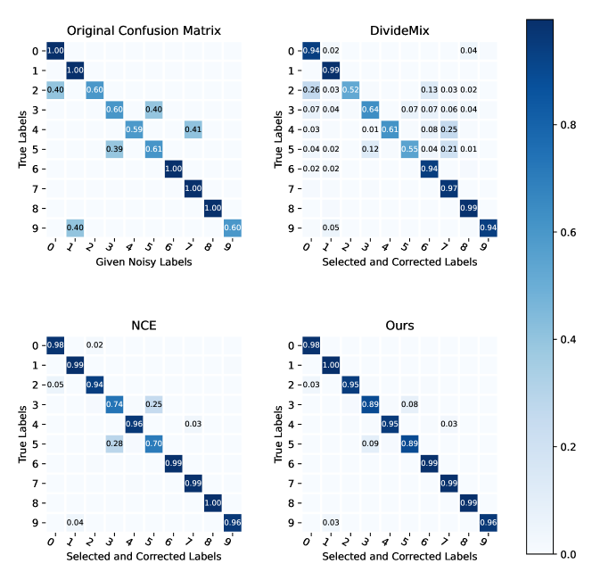
Figure S7: Comparision of confusion matrix on CIFAR-10 assym-40%. The darker the color on the diagonal elements of the matrix, the higher the accuracy.

As shown in Tab. 4 (h), only training with identified clean labels leads to inferior model performance. Furthermore, replacing our CSOT-based denoising and relabeling with confidence thresholding (CT) [62] for corrupted label correction also degrades the model performance, as shown in Tab. 4 (i). The CT methods assign pseudo labels to samples based on model prediction, which is unreliable in the early training stage, especially under high noise rates. Our CSOT-based denoising and relabeling fully consider the inter- and intra-distribution structure of samples, yielding more robust labels. Particularly, our CSOT outperforms NCE and DivideMix significantly in label correction, as demonstrated by the superior corrected accuracy in Fig. 2(b) and the improved clarity of the confusion matrix in Fig. S7.

Table 4: Ablation studies under multiple label noise ratios on CIFAR-10 and CIFAR-100. "repl." is an abbreviation for "replaced", and $\mathcal{L}^{ce}$ represents a cross-entropy loss. GMM refers to the selection of clean labels based on small-loss criterion [46]. CT (confidence thresholding [62]) is a relabeling scheme where we set the CT value to 0.95.

	Dataset	CIFAR-10				CIFAR-100			Avg
	Noise type	Sym.			Asym.	Sym.
	Method/Noise ratio	0.5	0.8	0.9	0.4	0.5	0.8	0.9
Denoise Relabeling Technique	(a) Classical OT	95.45	91.95	82.35	95.04	75.96	62.46	43.28	78.07
	(b) Structure-aware OT	95.86	91.87	83.29	95.06	76.20	63.73	44.57	78.65
	(c) CSOT w/o $\Omega^{\mathbf{P}}$ and $\Omega^{\mathbf{L}}$	95.53	93.84	89.50	95.14	75.96	66.50	47.55	80.57
	(d) CSOT w/o $\Omega^{\mathbf{P}}$	95.77	94.08	89.97	95.35	76.09	66.79	48.13	80.88
	(e) CSOT w/o $\Omega^{\mathbf{L}}$	95.55	93.97	90.41	95.15	76.17	67.28	48.01	80.93
Learning Technique	(f) GMM + $\mathcal{L}^{sup}$	92.48	80.37	31.76	90.80	69.52	48.49	20.86	62.04
	(g) CSOT repl. $\mathcal{L}^{sup}$ with $\mathcal{L}^{ce}$	93.47	81.93	53.45	91.43	72.66	50.62	21.77	66.48
	(h) CSOT w/o $\mathcal{L}^{semi}$	95.34	93.04	88.9	94.11	75.16	61.13	36.94	77.80
	(i) CSOT repl. correction with CT (0.95)	95.46	90.73	89.09	95.21	75.85	64.28	48.76	79.91
	(j) CSOT w/o $\mathcal{L}^{simsiam}_{\mathcal{D}_{corrupted}}$	95.92	94.17	89.31	95.16	76.38	66.17	45.56	80.38
	CSOT	96.20	94.39	90.65	95.50	77.94	67.78	50.50	81.85

Effectiveness of curriculum training scheme.

According to the progressive clean and corrupted accuracy during the training process shown in Fig. 2(a) and Fig. 2(b), our curriculum identification scheme ensures high accuracy in the early training stage, avoiding overfitting to wrong corrected labels. Note that since our model is trained using only a fraction of clean samples, it is crucial to employ a powerful supervised learning loss to facilitate better learning. Otherwise, the performance will be poor without the utilization of a powerful supervised training loss, as evidenced in Tab. 4 (g). In addition, the incorporation of self-supervised loss enhances noise-robust representation, particularly in high noise rate scenarios, as demonstrated in our experiments in Tab. 4 (j).

Time cost discussion for solving CSOT

To verify the efficiency of our proposed lightspeed scaling iteration, we conduct some experiments for solving CSOT optimization problem of different input sizes on a single GPU NVIDIA A100. As demonstrated in Tab. 3, our proposed lightspeed computational method that involves an efficient scaling iteration (Algorithm 1) achieves lower time cost compared to vanilla Dykstra’s algorithm (Algorithm S6). Specifically, compared to the vanilla Dykstra-based approach, our efficient scaling iteration version can achieve a speedup of up to 3.7 times, thanks to efficient matrix-vector multiplication instead of matrix-matrix multiplication. Moreover, even for very large input sizes, the computational time cost does not increase significantly.

7 Conclusion and Limitation

In this paper, we proposed Curriculum and Structure-aware Optimal Transport (CSOT), a novel solution to construct robust denoising and relabeling allocator that simultaneously considers the inter- and intra-distribution structure of samples. Unlike current approaches, which rely solely on the model’s predictions, CSOT considers the global and local structure of the sample distribution to construct a robust denoising and relabeling allocator. During the training process, the allocator assigns reliable labels to a fraction of the samples with high confidence, ensuring both global discriminability and local coherence. To efficiently solve CSOT, we developed a lightspeed computational method that involves a scaling iteration within a generalized conditional gradient framework. Extensive experiments on three benchmark datasets validate the efficacy of our proposed method. While class-imbalance cases are not considered in this paper within the context of LNL, we believe that our approach can be further extended for this purpose.

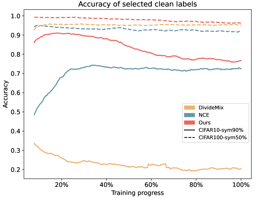
(a) Clean accuracy

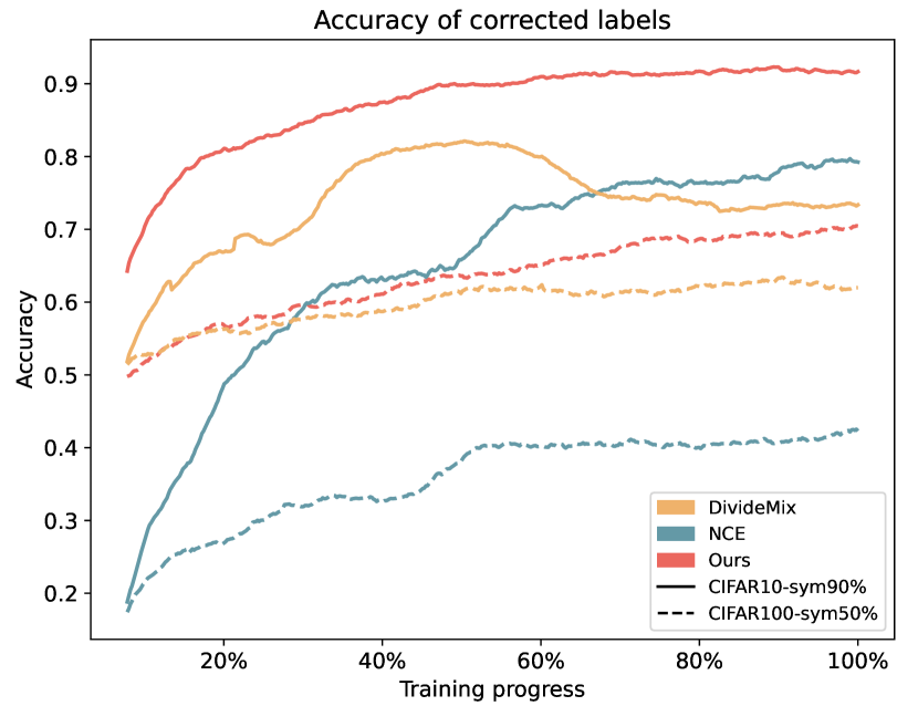
(b) Corrected accuracy

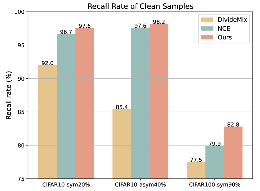
(c) Clean recall rate

Figure 2: Performance comparison for clean label identification and corrupted label correction.

8 Acknowledgement

This work was supported by NSFC (No.62303319), Shanghai Sailing Program (21YF1429400, 22YF1428800), Shanghai Local College Capacity Building Program (23010503100), Shanghai Frontiers Science Center of Human-centered Artificial Intelligence (ShangHAI), MoE Key Laboratory of Intelligent Perception and Human-Machine Collaboration (ShanghaiTech University), and Shanghai Engineering Research Center of Intelligent Vision and Imaging.

Appendix A Supplement for Training Details

A.1 Implementation Details

CIFAR10/100.

Following previous works [46, 45], we use PreAct ResNet-18 [34] as the backbone, and train it using SGD with a momentum of 0.9, a weight decay of 0.0005, and a batch size of 128. We set the initial learning rate as 0.02, with a cosine learning rate decay schedule. The hidden layer in SimSiam projection MLP is set to 128-d.

Webvision.

Following previous works [46, 45], we use inception-resnet v2 [64] as the backbone, and train it using SGD with a momentum of 0.9, a weight decay of 0.0005, and a batch size of 32. We set the initial learning rate as 0.01, with a cosine learning rate decay schedule. The hidden layer in SimSiam projection MLP is set to 384-d.

Other details.

All experiments are implemented on a single GPU of NVIDIA A100 with 80 GB memory. We follow DivideMix [46] and NCE [45] to set the hyper-parameters in the mixup loss and label consistency loss. The loss trade-off weights $\lambda_{1}$ and $\lambda_{2}$ are empirically set to $1$, which is similar to NCE [45]. The selection criterion of the hyper-parameters $\varepsilon$ and $\kappa$ in CSOT formulation is analyzed in Sec. B.5. Our code is modified based on DivideMix [46] https://github.com/LiJunnan1992/DivideMix and NCE [45] https://github.com/lijichang/LNL-NCE. The CSOT solver code is modified based on POT [26].

A.2 Training Loss

To be self-contained, we specify the Mixup loss $\mathcal{L}^{mix}$ and label consistency loss $\mathcal{L}^{lab}$ adopted in NCE [45], and the self-supervised loss $\mathcal{L}^{simsiam}$ proposed in SimSiam [15].

Mixup loss.

Mixup [81] can effectively mitigate noise memorization, and thus mixup regularization can be used to construct augmented samples through linear combinations of existing samples from $\mathcal{D}_{clean}$. Given two existing samples $(\mathbf{x}_{i},y_{i})$ and $(\mathbf{x}_{j},y_{j})$ from $\mathcal{D}_{clean}$, an augmented sample $\widetilde{\mathbf{x}},\widetilde{y}$ can be generated as follows:

$$\widetilde{\mathbf{x}}=\gamma\mathbf{x}_{i}+(1-\gamma)\mathbf{x}_{j},\quad\widetilde{y}=\gamma p_{y}(y_{i})+(1-\gamma)p_{y}(y_{j}),$$ (S17)

where $p_{y}(y_{i})$ is the one-hot vector for the given label $y_{i}$ and $\gamma\sim Beta(\alpha)$ is a mixup ratio and $\alpha$ is a scalar parameter of Beta distribution. The cross-entropy loss applied to $B^{\prime}$ augmented samples in each training mini-batch is defined as follows:

$$\mathcal{L}^{mix}=-\frac{1}{B^{\prime}}\sum_{i=1}^{B^{\prime}}\widetilde{y}_{i}\log p(y|\widetilde{\mathbf{x}}_{i}),$$ (S18)

where $p(y|\widetilde{\mathbf{x}}_{b})$ is the softmax prediction of a mixup input $\widetilde{\mathbf{x}}_{b}$.

Label consistency loss.

Label consistency regularization encourages the fine-tuned model to produce the same output when there are minor perturbations in the input [62]. Hence consistency regularization can be used to further enhance the robustness of the model [22]. The label consistency is enforced by minimizing the following loss:

$$\mathcal{L}^{lab}=-\frac{1}{B^{\prime}}\sum_{i=1}^{B^{\prime}}p_{y}(y_{i})\log p(y|\textbf{Aug}(x_{i})),$$ (S19)

where $\textbf{Aug}(\cdot)$ denotes the function that perturbs the chosen samples using Autoaugment technique proposed in [18].

SimSiam loss.

We simply define a feature extractor as $f$ and a projection layer as $h$. Given two augmented views $\mathbf{x}_{i}^{1}$ and $\mathbf{x}_{i}^{2}$ from an image $\mathbf{x}$, we can have $p_{i}^{1}=h(f(\mathbf{x}_{i}^{1}))$ and $z_{i}^{2}=f(\mathbf{x}_{i}^{2})$. The negative cos similarity is defined as follows:

$$\ell(p_{i}^{1},z_{i}^{2})=-\frac{p_{i}^{1}z_{i}^{2}}{\left\|p_{i}^{1}\right\|_{2}\left\|z_{i}^{2}\right\|_{2}}$$ (S20)

where $\left\|\cdot\right\|_{2}$ is $\ell_{2}$-norm. To construct the contrastive loss by enforcing the consistency between two positive pairs $(p_{i}^{1},z_{i}^{2})$ and $(p_{i}^{2},z_{i}^{1})$, the SimSiam loss is defined as follows:

$$\mathcal{L}^{simsiam}=-\frac{1}{2B^{\prime}}\sum_{i=1}^{B^{\prime}}\big{(}\ell(p_{i}^{1},\texttt{stopgrad}(z_{i}^{2}))+\ell(p_{i}^{2},\texttt{stopgrad}(z_{i}^{1}))\big{)}$$ (S21)

where $\texttt{stopgrad}(\cdot)$ is a stop-gradient operation that can be easily realized by .detach() operation in PyTorch.

A.3 Training Process

Algorithm S3 Training process of proposed CSOT

1:  Input: Training dataset $\mathcal{D}_{train}$, number of warmup training epochs $T_{warm}$ , number of supervised training epochs $T_{sup}$, number of semi-supervised training epochs $T_{semi}$, initial curriculum budget $m_{0}$.

2:  Initialize model parameter $\theta$.

3:  for $t=1,\ldots,(T_{sup}+T_{semi})$ do

4:     if $t<T_{warm}$ then

5:        WarmUp($\mathcal{D}_{train}$; $\theta$).

6:     else

7:        Compute the curriculum budget $m=\min(1.0,m_{0}+\frac{t-1}{T_{sup}-1})$.

8:        for $b=1,\ldots,N_{batch}^{relabeling}$ do

9:           Draw a mini-batch $\mathcal{X}_{b}$ from $\mathcal{D}_{train}$.

10:           Denoising and relabeling for $\mathcal{X}_{b}$: solve the Problem (LABEL:eq:CSOT) by Algorithm 2.

11:        end for

12:        Use Eq. 8 to split the training dataset $\mathcal{D}_{train}$ into the clean dataset $\mathcal{D}_{clean}$ and the corrupted dataset $\mathcal{D}_{currupted}$.

13:        for $b^{\prime}=1,\ldots,N_{batch}^{train}$ do

14:           Draw a mini-batch $\mathcal{X}_{b^{\prime}}$ from $\mathcal{D}_{clean}$, and draw a mini-batch $\mathcal{U}_{b^{\prime}}$ from $\mathcal{D}_{currupted}$.

15:           if $t<T_{sup}$ then

16:              $\mathcal{L}=\mathcal{L}^{mix}_{\mathcal{X}_{b^{\prime}}}+\mathcal{L}^{lab}_{\mathcal{X}_{b^{\prime}}}+\lambda_{1}\mathcal{L}^{simsiam}_{\mathcal{U}_{b^{\prime}}}$.

17:           else

18:              $\mathcal{L}=\mathcal{L}^{mix}_{\mathcal{X}_{b^{\prime}}}+\mathcal{L}^{lab}_{\mathcal{X}_{b^{\prime}}}+\lambda_{2}\mathcal{L}^{lab}_{\mathcal{U}_{b^{\prime}}}$.

19:           end if

20:           Update model parameter $\theta$ by applying SGD with loss $\mathcal{L}$.

21:        end for

22:     end if

23:  end for

24:  Return: Optimal model parameter $\theta$.

We specify our training process in Algorithm S3, which mainly includes two parts, i.e. denoising and relabeling part, the training part.

Appendix B Supplement for Experimental Results

B.1 Comparison with Prediction- , OT- and SOT-Based Pseudo-Labeling

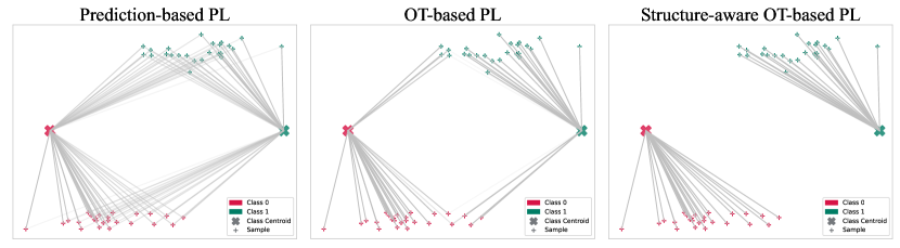
(a) Illustrations of different pseudo-labeling mappings.

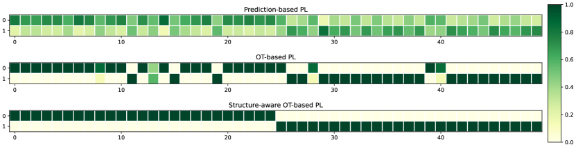
(b) Illustrations of different pseudo-labeling (transposed) coupling matrices.

Figure S3: Comparison with prediction- , OT- and SOT-based pseudo-labeling. We consider a toy binary classification case for simplicity.

As shown in Fig. 3(a) and 3(b), prediction-based PL generates vague predictions when the class centroids are not discriminative enough. To explain this, prediction-based PL assigns labels in a per-class manner without considering either the global structure of the sample distribution. To this end, OT-based PL optimizes the mapping problem considering the inter-distribution matching of samples and classes, and thus produces more discriminative labels. However, as shown in Fig. 3(a), two nearby samples could be mapped to two far-away class centroids, which is not reasonable since it overlooks the inherent coherence structure of the sample distribution, i.e. intra-distribution coherence. Therefore, our proposed SOT encourages generating more robust labels with both global discriminability and local coherence.

B.2 Visualization of the Coupling Matrix for CSOT

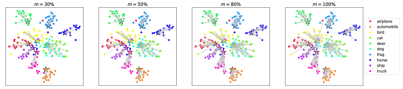
(a) Illustrations of CSOT mappings with different curriculum budgets $m$.

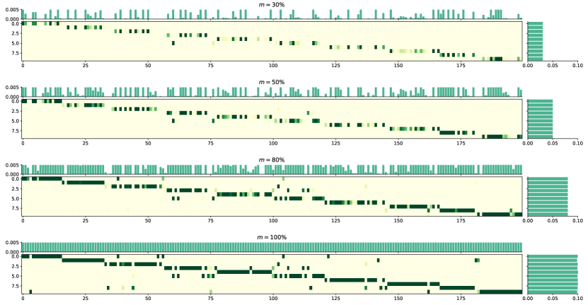
(b) Illustrations of CSOT (transposed) coupling matrices with different curriculum budgets $m$.

Figure S4: Comparison with using different curriculum budgets $m$. The samples are plotted as colorful dots and the class centroids are plotted as five-pointed stars, which are colored by their true labels.

We visualize randomly selected 200 samples of CIFAR-10 (after 10-epoch warm-up training) and 10 implicit class centroids in feature space in Fig. 4(a). The feature dots are visualized based on t-SNE [66], and the implicit class centroids are obtained by a weighted sum of the softmax prediction scores. It is evident that the feature space exhibits confusion in the early training stage, particularly among semantically similar classes, such as cat and dog. Therefore, utilizing a full mapping based on OT would lead to incorrect assignments for samples that have not yet been sufficiently learned. Our proposed strategy, on the other hand, demonstrates superiority by selectively assigning reliable labels to a fraction of samples with the highest confidence. This approach ensures high training label accuracy and mitigates the negative impact of unreliable labels during the early stages of training. In addition, we also visualize the coupling matrices, along with their corresponding row and column sum vectors by histograms in Fig. 4(b), which illustrates the partial mapping controlled by curriculum constraints.

B.3 Convergence of the proposed GCG algorithm for CSOT

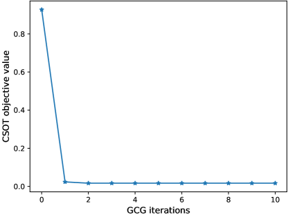
Figure S5: Convergence behaviour of the generalized conditional gradient (GCG) algorithm for CSOT.

We set the number of outer loops is set to 10, and the number for inner scaling iteration is set to 100. And the curriculum budget $m$ is set to $0.5$, and the local coherent regularized terms weight $\kappa$ is set to $1$. As demonstrated in Fig. S5, our computational method, which includes a novel scaling iteration within a generalized conditional gradient framework, is capable of optimizing the non-convex objective and converging to a stationary point.

B.4 Addictional Results of CSOT

Effectiveness of CSOT-based denoising and relabeling.

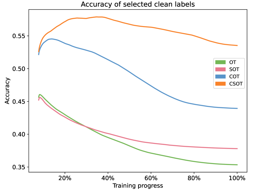
(a) Clean accuracy

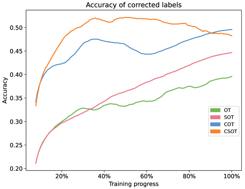
(b) Corrected accuracy

Figure S6: Performance comparison for clean label identification and corrupted label correction. The experiments are conducted on CIFAR-100 sym0.9.

Method	Time cost
DivideMix[46]	5.1h
NCE[45]	6.5h
CSOT	4.8h

Table S5: Comparison of total training time (hours) on CIFAR-10.The experiments are implemented on a single GPU NVIDIA A100.

To further verify the effectiveness of our CSOT for clean label identification and corrupted label correction, we also conduct ablation experiments on OT-, SOT-, COT-, and CSOT-based denoising and relabeling. As depicted in Fig. S6, the incorporation of curriculum constraints ensures high accuracy of clean labels during the early training stage. This, in turn, facilitates effective learning by providing the model with correct and reliable information, which avoids error accumulation. Furthermore, local coherent regularized terms contribute to improved label correction.

Result of Clothing1M.

Table S6: Comparison with state-of-the-art methods in test accuracy (%) on Clothing1M.

Method	Meta-L. [47]	DivideMix [46]	ELR+ [50]	ELR+ [50]	RRL [48]	NCE‡ [45]	CSOT
Accuracy	73.50	74.48	72.87	74.80	74.84	74.71	75.16

Clothing1M [74] is another real-world noisy dataset, which consists of 1 million training images collected from online shopping websites with labels generated from surrounding texts. We use the augmentation provided in [62] as $\textbf{Aug}(\cdot)$. Following the similar setting in NCE [45] and DivideMix [46], we also conduct the experiment on Clothing1M and achieve superior performance compared to existing approaches, as shown in Tab. S6. Since NCE utilized an inaccessible data augmentation and hence we reproduce NCE with the augmentation in [62] for a fair comparison, denoted by ‡.

B.5 Hyperparameter Analysis

Entropic regularized weight $\varepsilon$.

Figure S8: Visualization of coupling matrix with different entropic regularized weights $\varepsilon$. We conduct experiments on randomly selected 200 samples of CIFAR-10 (after 10-epoch warm-up training) and the curriculum budget $m$ is set to $0.5$.

When $\varepsilon\to 0$, the entropic regularized CSOT formulation becomes closer to the exact CSOT. Therefore, in order to obtain a solution that closely approximates the exact CSOT, we prefer to set $\varepsilon$ to a small value. We visualize the coupling matrix with different $\varepsilon$ in Fig. S8, and it can be observed that the $\varepsilon$ also influences the mapping smoothness. A smaller $\varepsilon$ leads to sharper pseudo labels. To ensure discriminative relabeling and reliable selection, we set $\varepsilon$ to 0.1.

Local coherent regularized weight $\kappa$.

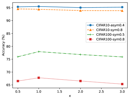
Figure S9: Sensitivity to the local coherent regularized weight $\kappa$ on four different noisy learning tasks.

The local coherent regularized weight, $\kappa$, determines the strength of local coherent mapping. As shown in Fig. S9, we can observe that the performance is not sensitive to the different values of $\kappa$, and it is relatively easy to tune. It is important to note that setting $\kappa$ too high can result in performance degradation, particularly in scenarios with high noise rates. This is because the label-level local consistency term $\Omega^{\mathbf{L}}$, may introduce incorrect consistency in such cases.

Appendix C More Discussion about CSOT

Appendix D Background on Computational Optimal Transport

D.1 Sinkhorn’s Algorithm

Algorithm S4 Sinhorn algorithm, for entropic regularized classical OT

1:  Input: Cost matrix $\mathbf{C}$, marginal constraints vectors $\bm{\alpha}$ and $\bm{\beta}$, entropic regularization weight $\varepsilon$

2:  Initialize: $\mathbf{K}\leftarrow e^{-\mathbf{C}/\varepsilon}$, $\bm{v}^{(0)}\leftarrow\mathds{1}_{|\bm{\beta}|}$

3:  Compute: $\mathbf{K}_{\bm{\alpha}}\leftarrow\frac{\mathbf{K}}{\text{diag}(\bm{\alpha})\mathds{1}_{|\bm{\alpha}|\times|\bm{\beta}|}}$, $\mathbf{K}_{\bm{\beta}}^{\top}\leftarrow\frac{\mathbf{K}^{\top}}{\text{diag}(\bm{\beta})\mathds{1}_{|\bm{\beta}|\times|\bm{\alpha}|}}$ // Saving computation

4:  for $n=1,2,3,\ldots$ do

5:     $\bm{u}^{(n)}\leftarrow\frac{\mathds{1}_{|\bm{\alpha}|}}{\mathbf{K}_{\bm{\alpha}}\bm{v}^{(n-1)}}$

6:     $\bm{v}^{(n)}\leftarrow\frac{\mathds{1}_{|\bm{\beta}|}}{\mathbf{K}_{\bm{\beta}}^{\top}\bm{u}^{(n)}}$

7:  end for

8:  Return: $\text{diag}(\bm{u}^{(n)})\mathbf{K}\text{diag}(\bm{v}^{(n)})$

The Sinkhorn algorithm for solving entropic regularized OT problem is presented in Algorithm S4. It is evident that our proposed scaling iteration is very similar to the existing efficient Sinkhorn algorithm. The main difference lies in Line 5 of Algorithm S4, which corresponds to Line 5 of Algorithm 1. Therefore, our scaling iteration shares the same quadratic time complex as the Sinkhorn algorithm.

D.2 Relation Between Kullback-Leibler Divergence and Entropic Regularized OT

Given a convex set $\mathcal{C}$, and a matrix $\mathbf{M}$, the projection according to the Kullback-Leibler (KL) divergence is defined as

$$P^{\text{KL}}_{\mathcal{C}}(\mathbf{M})\overset{\underset{\mathrm{def}}{}}{=}\operatorname*{argmin}_{\mathbf{Q}\in\mathcal{C}}\text{KL}(\mathbf{Q}|\mathbf{M}).$$ (S22)

According to [8], the classical OT can be rewritten in a KL projection form as follows:

$$\min_{\mathbf{Q}\in\mathbf{\Pi}(\bm{\alpha},\bm{\beta})}\left<\mathbf{C},\mathbf{Q}\right>=\min_{\mathbf{Q}\in\mathbf{\Pi}(\bm{\alpha},\bm{\beta})}\varepsilon\text{KL}(\mathbf{Q}|e^{-\mathbf{C}/\varepsilon}),$$ (S23)

which can be interpreted as that solving a classical OT problem is equivalent to solving a KL projection from a given matrix $e^{-\mathbf{C}/\varepsilon}$ to the constraint $\mathbf{\Pi}(\bm{\alpha},\bm{\beta})$. In light of this, it was proposed in [8] that when $\mathcal{C}$ is an intersection of closed convex and affine sets, the classical OT problem can be solved by iterative Bregman projections [10]. However, when $\mathcal{C}$ is an intersection of closed convex but not affine sets, Dykstra’s algorithm [21] is employed to guarantee convergence [7], as iterative Bregman projections do not generally converge to the KL projection on the intersection.

D.3 Dykstra’s Algorithm

Assume that $\mathcal{C}$ is an intersection of closed convex but not affine sets:

$$\mathcal{C}=\bigcap_{\ell=1}^{L}\mathcal{C}_{\ell},$$ (S24)

and we extend the indexing of the sets by $L$-periodicity so that they satisfy

$$\forall n\in\mathbb{N},\quad\mathcal{C}_{n+L}=\mathcal{C}_{n}.$$ (S25)

Dykstra’s algorithm [21] starts by initializing

$$\mathbf{Q}^{(0)}=\mathbf{K}\quad\text{and}\quad\mathbf{U}^{(0)}=\mathbf{U}^{(-1)}=\cdots=\mathbf{U}^{(-L+1)}=\mathds{1}.$$ (S26)

One then iteratively defines

$$\mathbf{Q}^{(n)}=P^{\text{KL}}_{\mathcal{C}_{n}}(\mathbf{Q}^{(n-1)}\odot\mathbf{U}^{(n-L)}),\quad\text{and}\quad\mathbf{U}^{(n)}=\mathbf{U}^{(n-L)}\odot\frac{\mathbf{Q}^{(n-1)}}{\mathbf{Q}^{(n)}}.$$ (S27)

D.4 Generalized Conditional Gradient Algorithm

We are interested in the problem of minimizing under constraints a composite function such as

$$\min_{\mathbf{Q}\in\mathcal{C}}=f(\mathbf{Q})+g(\mathbf{Q}),$$ (S28)

where both $f(\cdot)$ is a differentiable and possibly non-convex function; $g(\cdot)$ is a convex, possibly non-differentiable function; $\mathcal{C}$ denotes any convex and compact set. One might want to benefit from this composite structure during the optimization procedure. For instance, if we have an efficient solver for optimizing

$$\min_{\mathbf{Q}\in\mathcal{C}}=\left<\nabla f,\mathbf{Q}\right>+g(\mathbf{Q}).$$ (S29)

It is of prime interest to use this solver in the optimization scheme instead of linearizing the whole objective function as one would do with a conditional gradient algorithm [9, 59], as shown in Algorithm S5.

Algorithm S5 Generalized conditional gradient algorithm

1:  Input: A differentiable and possibly non-convex function $f$ and its gradient function $\nabla f$, a convex, possibly non-differentiable function $g$, a convex and compact set $\mathcal{C}$.

2:  Initialize: $\mathbf{Q}^{(0)}\in\mathcal{C}$

3:  for $i=1,2,3,\ldots$ do

4:     $\mathbf{G}^{(i)}\leftarrow\mathbf{Q}^{(i)}+\nabla f(\mathbf{Q}^{(i)})$ // Gradient computation

5:     $\widetilde{\mathbf{Q}}^{(i)}\leftarrow\operatorname*{argmin}_{\mathbf{Q}\in\mathcal{C}}\left<\mathbf{Q},\mathbf{G}^{(i)}\right>+g(\mathbf{Q})$ // Partial linearization

6:     Find the optimal step $\eta^{(i)}$ with $\Delta\mathbf{Q}=\widetilde{\mathbf{Q}}^{(i)}-\mathbf{Q}^{(i)}$

$$\eta^{(i)}=\operatorname*{argmin}_{\eta\in[0,1]}f(\mathbf{Q}^{(i)}+\eta^{(i)}\Delta\mathbf{Q})+g(\mathbf{Q}^{(i)}+\eta^{(i)}\Delta\mathbf{Q})$$

or choose $\eta^{(i)}\in[0,1]$ so that it satisfies the Armijo rule.// Exact or backtracking line-search

7:     $\mathbf{Q}^{(i+1)}\leftarrow\left(1-\eta^{(i)}\right)\mathbf{Q}^{(i)}+\eta^{(i)}\widetilde{\mathbf{Q}}^{(i)}$ // Update

8:  end for

9:  Return: $\mathbf{Q}^{(i)}$

Appendix E Derivation Details of the Efficient Scaling Iteration Method (Lemma 1)

We have developed a lightspeed computational method that involves a scaling iteration within a generalized conditional gradient framework to solve CSOT efficiently. Specifically, the efficiency is mainly brought by the scaling iteration method for solving the COT problem (Problem (12)), which is proposed in Lemma 1.

This section presents the derivation details of this efficient scaling iteration method. First, we show that solving COT is equivalent to solving the KL projection problem with the curriculum constraints (Lemma S2). Then such a KL projection problem can be solved by iterating Dykstra’s algorithm (Lemma S3). However, Dykstra’s algorithm is based on matrix-matrix multiplication which is computationally extensive. Therefore, we propose a fast implementation of Dykstra’s algorithm by only performing matrix-vector multiplications, i.e. efficient scaling iteration (Lemma 1).

Lemma S2.

Solving the Problem (12) is equivalent to solving the KL projection problem from the matrix $e^{-\mathbf{C}/\varepsilon}$ to the curriculum constraint $\mathbf{\Pi}^{\text{c}}(\bm{\alpha},\bm{\beta})$, i.e.

$$\min_{\mathbf{Q}\in\mathbf{\Pi}^{\text{c}}(\bm{\alpha},\bm{\beta})}\left<\mathbf{C},\mathbf{Q}\right>+\varepsilon\left<\mathbf{Q},\log\mathbf{Q}\right>\Leftrightarrow\min_{\mathbf{Q}\in\mathbf{\Pi}^{\text{c}}(\bm{\alpha},\bm{\beta})}\varepsilon\text{KL}(\mathbf{Q}|e^{-\mathbf{C}/\varepsilon}),$$ (S30)

Proof.

$$\quad\,\min_{\mathbf{Q}\in\mathbf{\Pi}^{\text{c}}(\bm{\alpha},\bm{\beta})}\left<\mathbf{C},\mathbf{Q}\right>+\varepsilon\left<\mathbf{Q},\log\mathbf{Q}\right>$$

$$=\min_{\mathbf{Q}\in\mathbf{\Pi}^{\text{c}}(\bm{\alpha},\bm{\beta})}\left<\mathbf{Q},\mathbf{C}+\varepsilon\log\mathbf{Q}\right>$$

$$=\min_{\mathbf{Q}\in\mathbf{\Pi}^{\text{c}}(\bm{\alpha},\bm{\beta})}\varepsilon\left<\mathbf{Q},\mathbf{C}/\varepsilon+\log\mathbf{Q}\right>$$

$$=\min_{\mathbf{Q}\in\mathbf{\Pi}^{\text{c}}(\bm{\alpha},\bm{\beta})}\varepsilon\left<\mathbf{Q},\log\frac{\mathbf{Q}}{e^{-\mathbf{C}/\varepsilon}}\right>$$

$$=\min_{\mathbf{Q}\in\mathbf{\Pi}^{\text{c}}(\bm{\alpha},\bm{\beta})}\varepsilon\text{KL}(\mathbf{Q}|e^{-\mathbf{C}/\varepsilon})$$

∎

Recall that the curriculum constraints $\mathbf{\Pi}^{\text{c}}(\bm{\alpha},\bm{\beta})$ can be expressed as an intersection of two convex but not affine sets:

$$\mathcal{C}_{1}\overset{\underset{\mathrm{def}}{}}{=}\left\{\mathbf{Q}\in\mathbb{R}_{+}^{|\bm{\alpha}|\times|\bm{\beta}|}|\mathbf{Q}\mathds{1}_{|\bm{\beta}|}\leq\bm{\alpha}\right\}\quad\text{and}\quad\mathcal{C}_{2}\overset{\underset{\mathrm{def}}{}}{=}\left\{\mathbf{Q}\in\mathbb{R}_{+}^{|\bm{\alpha}|\times|\bm{\beta}|}|\mathbf{Q}^{\top}\mathds{1}_{|\bm{\alpha}|}=\bm{\beta}\right\}.$$ (S31)

Lemma S3.

The KL projection from a matrix $\mathbf{M}$ to the $\mathcal{C}_{1}$ and $\mathcal{C}_{2}$ are expressed as

$$P^{\text{KL}}_{\mathcal{C}_{1}}(\mathbf{M})={\rm{diag}}\left(\min\left(\frac{\bm{\alpha}}{{\mathbf{M}}\mathds{1}_{|\bm{\beta}|}},\mathds{1}_{|\bm{\beta}|}\right)\right){\mathbf{M}},$$ (S32)

$$P^{\text{KL}}_{\mathcal{C}_{2}}(\mathbf{M})={\mathbf{M}}{\rm{diag}}\left(\frac{\bm{\beta}}{{\mathbf{M}}^{\top}\mathds{1}_{|\bm{\alpha}|}}\right).$$ (S33)

Then the Problem (12) can be solved by Dykstra iterations, presented in Algorithm S6.

Lemma S3 can be derived form the Proposition 1 and Proposition 5 in [8].

Algorithm S6 Dykstra’s algorithm for entropic regularized Curriculum OT

1:  Input: Cost matrix $\mathbf{C}$, marginal constraints vectors $\bm{\alpha}$ and $\bm{\beta}$, entropic regularization weight $\varepsilon$

2:  Initialize: $\mathbf{Q}^{(0)}\leftarrow e^{-\mathbf{C}/\varepsilon}$, $\mathbf{U}^{\prime(0)}\leftarrow\mathds{1}_{|\bm{\alpha}|\times|\bm{\beta}|}$, $\mathbf{U}^{(0)}\leftarrow\mathds{1}_{|\bm{\alpha}|\times|\bm{\beta}|}$

3:  for $t=1,2,3,\ldots$ do

4:     $\mathbf{Q}^{\prime(t)}\leftarrow P^{\text{KL}}_{\mathcal{C}_{1}}(\mathbf{Q}^{(t-1)}\odot\mathbf{U}^{\prime(t-1)})$

5:     $\mathbf{U}^{\prime(t)}\leftarrow\mathbf{U}^{\prime(t-1)}\odot\frac{\mathbf{Q}^{(t-1)}}{\mathbf{Q}^{\prime(t)}}$

6:     $\mathbf{Q}^{(t)}\leftarrow P^{\text{KL}}_{\mathcal{C}_{2}}(\mathbf{Q}^{\prime(t)}\odot\mathbf{U}^{(t-1)})$

7:     $\mathbf{U}^{(t)}\leftarrow\mathbf{U}^{(t-1)}\odot\frac{\mathbf{Q}^{\prime(t)}}{\mathbf{Q}^{(t)}}$

8:  end for

9:  Return: $\mathbf{Q}^{(t)}$

The limitation of Dykstra’s algorithm comes from its computationally extensive matrix-matrix multiplication. To handle this issue, we propose a fast implementation of Dykstra’s algorithm by only performing matrix-vector multiplications, i.e. efficient scaling iteration (Lemma 1).

Lemma 1.

(Efficient scaling iteration for Curriculum OT) When solving Problem (12) by iterating Dykstra’s algorithm, the matrix $\mathbf{Q}^{(n)}$ at $n$ iteration is a diagonal scaling of $\mathbf{K}:=e^{-\mathbf{C}/\varepsilon}$, which is the element-wise exponential matrix of $-\mathbf{C}/\varepsilon$:

$$\mathbf{Q}^{(n)}={\rm{diag}}\left(\bm{u}^{(n)}\right)\mathbf{K}{\rm{diag}}\left(\bm{v}^{(n)}\right),$$ (S34)

where the vectors $\bm{u}^{(n)}\in\mathbb{R}^{|\bm{\alpha}|}$, $\bm{v}^{(n)}\in\mathbb{R}^{|\bm{\beta}|}$ satisfy $\bm{v}^{(0)}=\mathds{1}_{|\bm{\beta}|}$ and follow the recursion formula

$$\bm{u}^{(n)}=\min\left(\frac{\bm{\alpha}}{\mathbf{K}\bm{v}^{(n-1)}},\mathds{1}_{|\bm{\alpha}|}\right)\quad{\rm{and}}\quad\bm{v}^{(n)}=\frac{\bm{\beta}}{\mathbf{K}^{\top}\bm{u}^{(n)}}.$$ (S35)

Proof.

Firstly, let $\bm{u}^{(1)}:=\min\left(\frac{\bm{\alpha}}{\mathbf{Q}^{(0)}\mathds{1}_{|\bm{\beta}|}},\mathds{1}_{|\bm{\alpha}|}\right)$. Following the Algorithm S6 and Lemma S3, we derive $\mathbf{Q}^{\prime(1)}$ and $\mathbf{U}^{\prime(1)}$. Now we have

$$\mathbf{Q}^{\prime(1)}=P^{\text{KL}}_{\mathcal{C}_{1}}(\mathbf{Q}^{(0)}\odot\mathbf{U}^{\prime(0)})=\text{diag}\left(\min\left(\frac{\bm{\alpha}}{\mathbf{Q}^{(0)}\mathds{1}_{|\bm{\beta}|}},\mathds{1}_{|\bm{\alpha}|}\right)\right)\mathbf{Q}^{(0)}=\text{diag}\left(\bm{u}^{(1)}\right)\mathbf{Q}^{(0)},$$

$$\mathbf{U}^{\prime(1)}=\mathbf{U}^{\prime(0)}\odot\frac{\mathbf{Q}^{(0)}}{\mathbf{Q}^{\prime(1)}}=\frac{\mathbf{Q}^{(0)}}{\text{diag}\left(\bm{u}^{(1)}\right)\mathbf{Q}^{(0)}}=\text{diag}\left(1/\bm{u}^{(1)}\right)\mathds{1}_{|\bm{\alpha}|\times|\bm{\beta}|}.$$

Then let $\bm{v}^{(1)}:=\frac{\bm{\beta}}{\mathbf{Q}^{(0)\top}\bm{u}^{(1)}}$. And we derive $\mathbf{Q}^{(1)}$ and $\mathbf{U}^{(1)}$ as follows:

$$\mathbf{Q}^{(1)} =P^{\text{KL}}_{\mathcal{C}_{2}}(\mathbf{Q}^{\prime(1)}\odot\mathbf{U}^{(0)})$$

$$=\mathbf{Q}^{\prime(1)}\text{diag}\left(\frac{\bm{\beta}}{\mathbf{K}^{(1)\top}\mathds{1}_{|\bm{\alpha}|}}\right)$$

$$=\text{diag}\left(\bm{u}^{(1)}\right)\mathbf{Q}^{(0)}\text{diag}\left(\frac{\bm{\beta}}{\mathbf{Q}^{(0)\top}\text{diag}\left(\bm{u}^{(1)}\right)\mathds{1}_{|\bm{\alpha}|}}\right)$$

$$=\text{diag}\left(\bm{u}^{(1)}\right)\mathbf{Q}^{(0)}\text{diag}\left(\frac{\bm{\beta}}{\mathbf{Q}^{(0)\top}\bm{u}^{(1)}}\right)$$

$$=\text{diag}\left(\bm{u}^{(1)}\right)\mathbf{Q}^{(0)}\text{diag}\left(\bm{v}^{(1)}\right),$$

$$\mathbf{U}^{(1)}=\mathbf{U}^{(0)}\odot\frac{\mathbf{Q}^{\prime(1)}}{\mathbf{Q}^{(1)}}=\frac{\text{diag}\left(\bm{u}^{(1)}\right)\mathbf{Q}^{(0)}}{\text{diag}\left(\bm{u}^{(1)}\right)\mathbf{Q}^{(0)}\text{diag}\left(\bm{v}^{(1)}\right)}=\mathds{1}_{|\bm{\alpha}|\times|\bm{\beta}|}\text{diag}\left(1/\bm{v}^{(1)}\right).$$

For simplicity, before deriving $\mathbf{Q}^{\prime(2)}$ and $\mathbf{U}^{\prime(2)}$, we derive $\mathbf{Q}^{(1)}\odot\mathbf{U}^{\prime(1)}$ firstly:

$$\mathbf{Q}^{(1)}\odot\mathbf{U}^{\prime(1)} =\left(\text{diag}\left(\bm{u}^{(1)}\right)\mathbf{Q}^{(0)}\text{diag}\left(\bm{v}^{(1)}\right)\right)\odot\left(\text{diag}\left(1/\bm{u}^{(1)}\right)\mathds{1}_{|\bm{\alpha}|\times|\bm{\beta}|}\right)$$

$$=\left(\mathbf{Q}^{(0)}\text{diag}\left(\bm{v}^{(1)}\right)\right)\odot\left(\mathds{1}_{|\bm{\alpha}|\times|\bm{\beta}|}\right)$$

$$=\mathbf{Q}^{(0)}\text{diag}\left(\bm{v}^{(1)}\right).$$

Let $\bm{u}^{(2)}:=\min\left(\frac{\bm{\alpha}}{\mathbf{Q}^{(0)}\bm{v}^{(1)}},\mathds{1}_{|\bm{\alpha}|}\right)$. We can now derive $\mathbf{Q}^{\prime(2)}$ and $\mathbf{U}^{\prime(2)}$ as follows:

$$\mathbf{Q}^{\prime(2)} =P^{\text{KL}}_{\mathcal{C}_{1}}(\mathbf{Q}^{(1)}\odot\mathbf{U}^{\prime(1)})$$

$$=\text{diag}\left(\min\left(\frac{\bm{\alpha}}{\left(\mathbf{Q}^{(1)}\odot\mathbf{U}^{\prime(1)}\right)\mathds{1}_{|\bm{\beta}|}},\mathds{1}_{|\bm{\alpha}|}\right)\right)\left(\mathbf{Q}^{(1)}\odot\mathbf{U}^{\prime(1)}\right)$$

$$=\text{diag}\left(\min\left(\frac{\bm{\alpha}}{\mathbf{Q}^{(0)}\text{diag}\left(\bm{v}^{(1)}\right)\mathds{1}_{|\bm{\beta}|}},\mathds{1}_{|\bm{\alpha}|}\right)\right)\mathbf{Q}^{(0)}\text{diag}\left(\bm{v}^{(1)}\right)$$

$$=\text{diag}\left(\min\left(\frac{\bm{\alpha}}{\mathbf{Q}^{(0)}\bm{v}^{(1)}},\mathds{1}_{|\bm{\alpha}|}\right)\right)\mathbf{Q}^{(0)}\text{diag}\left(\bm{v}^{(1)}\right)$$

$$=\text{diag}\left(\bm{u}^{(2)}\right)\mathbf{Q}^{(0)}\text{diag}\left(\bm{v}^{(1)}\right),$$

$$\mathbf{U}^{\prime(2)} =\mathbf{U}^{\prime(1)}\odot\frac{\mathbf{Q}^{(1)}}{\mathbf{Q}^{\prime(2)}}$$

$$=\left(\text{diag}\left(1/\bm{u}^{(1)}\right)\mathds{1}_{|\bm{\alpha}|\times|\bm{\beta}|}\right)\odot\frac{\text{diag}\left(\bm{u}^{(1)}\right)\mathbf{Q}^{(0)}\text{diag}\left(\bm{v}^{(1)}\right)}{\text{diag}\left(\bm{u}^{(2)}\right)\mathbf{Q}^{(0)}\text{diag}\left(\bm{v}^{(1)}\right)}$$

$$=\left(\text{diag}\left(1/\bm{u}^{(1)}\right)\mathds{1}_{|\bm{\alpha}|\times|\bm{\beta}|}\right)\odot\frac{\text{diag}\left(\bm{u}^{(1)}\right)}{\text{diag}\left(\bm{u}^{(2)}\right)}$$

$$=\left(\text{diag}\left(1/\bm{u}^{(1)}\right)\mathds{1}_{|\bm{\alpha}|\times|\bm{\beta}|}\right)\odot\text{diag}\left(\bm{u}^{(1)}/\bm{u}^{(2)}\right)$$

$$=\text{diag}\left(1/\bm{u}^{(2)}\right)\mathds{1}_{|\bm{\alpha}|\times|\bm{\beta}|}.$$

For simplicity, before deriving $\mathbf{Q}^{(2)}$ and $\mathbf{U}^{(2)}$, we derive $\mathbf{Q}^{\prime(2)}\odot\mathbf{U}^{(1)}$ firstly:

$$\mathbf{Q}^{\prime(2)}\odot\mathbf{U}^{(1)} =\left(\text{diag}\left(\bm{u}^{(2)}\right)\mathbf{Q}^{(0)}\text{diag}\left(\bm{v}^{(1)}\right)\right)\odot\left(\mathds{1}_{|\bm{\alpha}|\times|\bm{\beta}|}\text{diag}\left(1/\bm{v}^{(1)}\right)\right)$$

$$=\left(\text{diag}\left(\bm{u}^{(2)}\right)\mathbf{Q}^{(0)}\right)\odot\mathds{1}_{|\bm{\alpha}|\times|\bm{\beta}|}$$

$$=\text{diag}\left(\bm{u}^{(2)}\right)\mathbf{Q}^{(0)}.$$

Let $\bm{v}^{(2)}:=\frac{\bm{\beta}}{\mathbf{Q}^{(0)\top}\bm{u}^{(2)}}$. We can now derive $\mathbf{Q}^{(2)}$ and $\mathbf{U}^{(2)}$ as follows:

$$\mathbf{Q}^{(2)} =P^{\text{KL}}_{\mathcal{C}_{2}}(\mathbf{Q}^{\prime(2)}\odot\mathbf{U}^{(1)})$$

$$=\text{diag}\left(\bm{u}^{(2)}\right)\mathbf{Q}^{(0)}\text{diag}\left(\frac{\bm{\beta}}{{(\text{diag}\left(\bm{u}^{(2)}\right)\mathbf{Q}^{(0)})}^{\top}\mathds{1}_{|\bm{\alpha}|}}\right)$$

$$=\text{diag}\left(\bm{u}^{(2)}\right)\mathbf{Q}^{(0)}\text{diag}\left(\frac{\bm{\beta}}{\mathbf{Q}^{(0)\top}\bm{u}^{(2)}}\right)$$

$$=\text{diag}\left(\bm{u}^{(2)}\right)\mathbf{Q}^{(0)}\text{diag}\left(\bm{v}^{(2)}\right)$$

$$\mathbf{U}^{(2)} =\mathbf{U}^{(1)}\odot\frac{\mathbf{Q}^{\prime(2)}}{\mathbf{Q}^{(2)}}$$

$$=\left(\mathds{1}_{|\bm{\alpha}|\times|\bm{\beta}|}\text{diag}\left(1/\bm{v}^{(1)}\right)\right)\odot\frac{\text{diag}\left(\bm{u}^{(2)}\right)\mathbf{Q}^{(0)}\text{diag}\left(\bm{v}^{(1)}\right)}{\text{diag}\left(\bm{u}^{(2)}\right)\mathbf{Q}^{(0)}\text{diag}\left(\bm{v}^{(2)}\right)}$$

$$=\left(\mathds{1}_{|\bm{\alpha}|\times|\bm{\beta}|}\text{diag}\left(1/\bm{v}^{(1)}\right)\right)\odot\frac{\text{diag}\left(\bm{v}^{(1)}\right)}{\text{diag}\left(\bm{v}^{(2)}\right)}$$

$$=\left(\mathds{1}_{|\bm{\alpha}|\times|\bm{\beta}|}\text{diag}\left(1/\bm{v}^{(1)}\right)\right)\odot\text{diag}\left(\bm{v}^{(1)}/\bm{v}^{(2)}\right)$$

$$=\mathds{1}_{|\bm{\alpha}|\times|\bm{\beta}|}\text{diag}\left(1/\bm{v}^{(2)}\right)$$

To conclude, it can be easily summarized that

$$\mathbf{Q}^{(n)}={\rm{diag}}\left(\bm{u}^{(n)}\right)\mathbf{K}{\rm{diag}}\left(\bm{v}^{(n)}\right),$$

where $\bm{u}^{(n)}=\min\left(\frac{\bm{\alpha}}{\mathbf{K}\bm{v}^{(n-1)}},\mathds{1}_{|\bm{\alpha}|}\right)$, $\bm{v}^{(n)}=\frac{\bm{\beta}}{\mathbf{K}^{\top}\bm{u}^{(n)}}$, and $\bm{v}^{(0)}=\mathds{1}_{|\bm{\beta}|}$.

∎

References

- [1] David Alvarez-Melis, Tommi Jaakkola, and Stefanie Jegelka. Structured optimal transport. In International conference on artificial intelligence and statistics, pages 1771–1780. PMLR, 2018.
- [2] Shuang Ao, Tianyi Zhou, Guodong Long, Qinghua Lu, Liming Zhu, and Jing Jiang. Co-pilot: Collaborative planning and reinforcement learning on sub-task curriculum. Advances in Neural Information Processing Systems, 34:10444–10456, 2021.
- [3] Eric Arazo, Diego Ortego, Paul Albert, Noel O’Connor, and Kevin McGuinness. Unsupervised label noise modeling and loss correction. In International conference on machine learning, pages 312–321. PMLR, 2019.
- [4] Devansh Arpit, Stanisław Jastrzębski, Nicolas Ballas, David Krueger, Emmanuel Bengio, Maxinder S Kanwal, Tegan Maharaj, Asja Fischer, Aaron Courville, Yoshua Bengio, et al. A closer look at memorization in deep networks. In International conference on machine learning, pages 233–242. PMLR, 2017.
- [5] YM Asano, C Rupprecht, and A Vedaldi. Self-labelling via simultaneous clustering and representation learning. In International Conference on Learning Representations, 2019.
- [6] Dara Bahri, Heinrich Jiang, and Maya Gupta. Deep k-nn for noisy labels. In International Conference on Machine Learning, pages 540–550. PMLR, 2020.
- [7] Heinz H Bauschke and Adrian S Lewis. Dykstras algorithm with bregman projections: A convergence proof. Optimization, 48(4):409–427, 2000.
- [8] Jean-David Benamou, Guillaume Carlier, Marco Cuturi, Luca Nenna, and Gabriel Peyré. Iterative bregman projections for regularized transportation problems. SIAM Journal on Scientific Computing, 37(2):A1111–A1138, 2015.
- [9] Dimitri P Bertsekas. Nonlinear programming. Journal of the Operational Research Society, 48(3):334–334, 1997.
- [10] Lev M Bregman. The relaxation method of finding the common point of convex sets and its application to the solution of problems in convex programming. USSR computational mathematics and mathematical physics, 7(3):200–217, 1967.
- [11] Mathilde Caron, Ishan Misra, Julien Mairal, Priya Goyal, Piotr Bojanowski, and Armand Joulin. Unsupervised learning of visual features by contrasting cluster assignments. Advances in neural information processing systems, 33:9912–9924, 2020.
- [12] Wanxing Chang, Ye Shi, Hoang Tuan, and Jingya Wang. Unified optimal transport framework for universal domain adaptation. Advances in Neural Information Processing Systems, 35:29512–29524, 2022.
- [13] Laetitia Chapel, Mokhtar Z Alaya, and Gilles Gasso. Partial optimal tranport with applications on positive-unlabeled learning. Advances in Neural Information Processing Systems, 33:2903–2913, 2020.
- [14] Pengfei Chen, Ben Ben Liao, Guangyong Chen, and Shengyu Zhang. Understanding and utilizing deep neural networks trained with noisy labels. In International Conference on Machine Learning, pages 1062–1070. PMLR, 2019.
- [15] Xinlei Chen and Kaiming He. Exploring simple siamese representation learning. In Proceedings of the IEEE/CVF conference on computer vision and pattern recognition, pages 15750–15758, 2021.
- [16] Ching-Yao Chuang, Stefanie Jegelka, and David Alvarez-Melis. Infoot: Information maximizing optimal transport. In International Conference on Machine Learning, pages 6228–6242. PMLR, 2023.
- [17] Nicolas Courty, Rémi Flamary, Devis Tuia, and Alain Rakotomamonjy. Optimal transport for domain adaptation. IEEE Transactions on Pattern Analysis and Machine Intelligence, 39:1853–1865, 2017.
- [18] Ekin D Cubuk, Barret Zoph, Dandelion Mane, Vijay Vasudevan, and Quoc V Le. Autoaugment: Learning augmentation strategies from data. In Proceedings of the IEEE/CVF conference on computer vision and pattern recognition, pages 113–123, 2019.
- [19] Marco Cuturi. Sinkhorn distances: Lightspeed computation of optimal transport. Advances in neural information processing systems, 26:2292–2300, 2013.
- [20] Jia Deng, Wei Dong, Richard Socher, Li-Jia Li, Kai Li, and Li Fei-Fei. Imagenet: A large-scale hierarchical image database. In 2009 IEEE conference on computer vision and pattern recognition, pages 248–255. Ieee, 2009.
- [21] Richard L Dykstra. An algorithm for restricted least squares regression. Journal of the American Statistical Association, 78(384):837–842, 1983.
- [22] Erik Englesson and Hossein Azizpour. Consistency regularization can improve robustness to label noise. In International Conference on Machine Learning Workshops, 2021 Workshop on Uncertainty and Robustness in Deep Learning, 2021.
- [23] Chuanwen Feng, Yilong Ren, and Xike Xie. Ot-filter: An optimal transport filter for learning with noisy labels. In Proceedings of the IEEE/CVF Conference on Computer Vision and Pattern Recognition, pages 16164–16174, 2023.
- [24] Sira Ferradans, Nicolas Papadakis, Gabriel Peyré, and Jean-François Aujol. Regularized discrete optimal transport. SIAM Journal on Imaging Sciences, 7(3):1853–1882, 2014.
- [25] Enrico Fini, Enver Sangineto, Stéphane Lathuilière, Zhun Zhong, Moin Nabi, and Elisa Ricci. A unified objective for novel class discovery. In Proceedings of the IEEE/CVF International Conference on Computer Vision, pages 9284–9292, 2021.
- [26] Rémi Flamary, Nicolas Courty, Alexandre Gramfort, Mokhtar Z. Alaya, Aurélie Boisbunon, Stanislas Chambon, Laetitia Chapel, Adrien Corenflos, Kilian Fatras, Nemo Fournier, Léo Gautheron, Nathalie T.H. Gayraud, Hicham Janati, Alain Rakotomamonjy, Ievgen Redko, Antoine Rolet, Antony Schutz, Vivien Seguy, Danica J. Sutherland, Romain Tavenard, Alexander Tong, and Titouan Vayer. Pot: Python optimal transport. Journal of Machine Learning Research, 22(78):1–8, 2021.
- [27] Marguerite Frank and Philip Wolfe. An algorithm for quadratic programming. Naval research logistics quarterly, 3(1-2):95–110, 1956.
- [28] Dandan Guo, Zhuo Li, He Zhao, Mingyuan Zhou, Hongyuan Zha, et al. Learning to re-weight examples with optimal transport for imbalanced classification. Advances in Neural Information Processing Systems, 35:25517–25530, 2022.
- [29] Lan-Zhe Guo and Yu-Feng Li. Class-imbalanced semi-supervised learning with adaptive thresholding. In International Conference on Machine Learning, pages 8082–8094. PMLR, 2022.
- [30] Sheng Guo, Weilin Huang, Haozhi Zhang, Chenfan Zhuang, Dengke Dong, Matthew R Scott, and Dinglong Huang. Curriculumnet: Weakly supervised learning from large-scale web images. In Proceedings of the European conference on computer vision, pages 135–150, 2018.
- [31] Bo Han, Quanming Yao, Xingrui Yu, Gang Niu, Miao Xu, Weihua Hu, Ivor Tsang, and Masashi Sugiyama. Co-teaching: Robust training of deep neural networks with extremely noisy labels. Advances in neural information processing systems, 31, 2018.
- [32] Kaiming He, Georgia Gkioxari, Piotr Dollár, and Ross Girshick. Mask r-cnn. In Proceedings of the IEEE international conference on computer vision, pages 2961–2969, 2017.
- [33] Kaiming He, Xiangyu Zhang, Shaoqing Ren, and Jian Sun. Deep residual learning for image recognition. In Proceedings of the IEEE conference on computer vision and pattern recognition, pages 770–778, 2016.
- [34] Kaiming He, Xiangyu Zhang, Shaoqing Ren, and Jian Sun. Identity mappings in deep residual networks. In European Conference on Computer Vision, pages 630–645. Springer, 2016.
- [35] Dan Hendrycks, Mantas Mazeika, Duncan Wilson, and Kevin Gimpel. Using trusted data to train deep networks on labels corrupted by severe noise. Advances in neural information processing systems, 31, 2018.
- [36] Martin Jaggi. Revisiting frank-wolfe: Projection-free sparse convex optimization. In International conference on machine learning, pages 427–435. PMLR, 2013.
- [37] Lu Jiang, Di Huang, Mason Liu, and Weilong Yang. Beyond synthetic noise: Deep learning on controlled noisy labels. In International conference on machine learning, pages 4804–4815. PMLR, 2020.
- [38] Lu Jiang, Deyu Meng, Qian Zhao, Shiguang Shan, and Alexander Hauptmann. Self-paced curriculum learning. In Proceedings of the AAAI Conference on Artificial Intelligence, volume 29, 2015.
- [39] Lu Jiang, Zhengyuan Zhou, Thomas Leung, Li-Jia Li, and Li Fei-Fei. Mentornet: Learning data-driven curriculum for very deep neural networks on corrupted labels. In International conference on machine learning, pages 2304–2313. PMLR, 2018.
- [40] Leonid V Kantorovich. On the translocation of masses. Journal of mathematical sciences, 133(4):1381–1382, 2006.
- [41] Nazmul Karim, Mamshad Nayeem Rizve, Nazanin Rahnavard, Ajmal Mian, and Mubarak Shah. Unicon: Combating label noise through uniform selection and contrastive learning. In Proceedings of the IEEE/CVF Conference on Computer Vision and Pattern Recognition, pages 9676–9686, 2022.
- [42] Faisal Khan, Bilge Mutlu, and Jerry Zhu. How do humans teach: On curriculum learning and teaching dimension. Advances in neural information processing systems, 24, 2011.
- [43] Alex Krizhevsky and Geoffrey Hinton. Learning multiple layers of features from tiny images. 2009.
- [44] Zhengfeng Lai, Chao Wang, Sen-ching Cheung, and Chen-Nee Chuah. Sar: Self-adaptive refinement on pseudo labels for multiclass-imbalanced semi-supervised learning. In Proceedings of the IEEE/CVF Conference on Computer Vision and Pattern Recognition, pages 4091–4100, 2022.
- [45] Jichang Li, Guanbin Li, Feng Liu, and Yizhou Yu. Neighborhood collective estimation for noisy label identification and correction. In European Conference on Computer Vision, pages 128–145. Springer, 2022.
- [46] Junnan Li, Richard Socher, and Steven CH Hoi. Dividemix: Learning with noisy labels as semi-supervised learning. In International Conference on Learning Representations, 2019.
- [47] Junnan Li, Yongkang Wong, Qi Zhao, and Mohan S Kankanhalli. Learning to learn from noisy labeled data. In Proceedings of the IEEE/CVF Conference on Computer Vision and Pattern Recognition, pages 5051–5059, 2019.
- [48] Junnan Li, Caiming Xiong, and Steven CH Hoi. Learning from noisy data with robust representation learning. In Proceedings of the IEEE/CVF International Conference on Computer Vision, pages 9485–9494, 2021.
- [49] Wen Li, Limin Wang, Wei Li, Eirikur Agustsson, and Luc Van Gool. Webvision database: Visual learning and understanding from web data. CoRR, 2017.
- [50] Sheng Liu, Jonathan Niles-Weed, Narges Razavian, and Carlos Fernandez-Granda. Early-learning regularization prevents memorization of noisy labels. Advances in neural information processing systems, 33:20331–20342, 2020.
- [51] Zhanyu Ma and Arne Leijon. Bayesian estimation of beta mixture models with variational inference. IEEE Transactions on Pattern Analysis and Machine Intelligence, 33(11):2160–2173, 2011.
- [52] Eran Malach and Shai Shalev-Shwartz. Decoupling" when to update" from" how to update". Advances in neural information processing systems, 30, 2017.
- [53] Sanmit Narvekar, Bei Peng, Matteo Leonetti, Jivko Sinapov, Matthew E Taylor, and Peter Stone. Curriculum learning for reinforcement learning domains: A framework and survey. The Journal of Machine Learning Research, 21(1):7382–7431, 2020.
- [54] Vu Nguyen, Sachin Farfade, and Anton van den Hengel. Confident sinkhorn allocation for pseudo-labeling. arXiv preprint arXiv:2206.05880, 2022.
- [55] Diego Ortego, Eric Arazo, Paul Albert, Noel E O’Connor, and Kevin McGuinness. Multi-objective interpolation training for robustness to label noise. In Proceedings of the IEEE/CVF Conference on Computer Vision and Pattern Recognition, pages 6606–6615, 2021.
- [56] Giorgio Patrini, Alessandro Rozza, Aditya Krishna Menon, Richard Nock, and Lizhen Qu. Making deep neural networks robust to label noise: A loss correction approach. In Proceedings of the IEEE conference on computer vision and pattern recognition, pages 1944–1952, 2017.
- [57] Haim Permuter, Joseph Francos, and Ian Jermyn. A study of gaussian mixture models of color and texture features for image classification and segmentation. Pattern recognition, 39(4):695–706, 2006.
- [58] Gabriel Peyré, Marco Cuturi, and Justin Solomon. Gromov-wasserstein averaging of kernel and distance matrices. In International conference on machine learning, pages 2664–2672. PMLR, 2016.
- [59] Alain Rakotomamonjy, Rémi Flamary, and Nicolas Courty. Generalized conditional gradient: analysis of convergence and applications. arXiv preprint arXiv:1510.06567, 2015.
- [60] Mengye Ren, Wenyuan Zeng, Bin Yang, and Raquel Urtasun. Learning to reweight examples for robust deep learning. In International conference on machine learning, pages 4334–4343. PMLR, 2018.
- [61] Shaoqing Ren, Kaiming He, Ross Girshick, and Jian Sun. Faster r-cnn: Towards real-time object detection with region proposal networks. Advances in neural information processing systems, 28, 2015.
- [62] Kihyuk Sohn, David Berthelot, Nicholas Carlini, Zizhao Zhang, Han Zhang, Colin A Raffel, Ekin Dogus Cubuk, Alexey Kurakin, and Chun-Liang Li. Fixmatch: Simplifying semi-supervised learning with consistency and confidence. Advances in neural information processing systems, 33:596–608, 2020.
- [63] Hwanjun Song, Minseok Kim, and Jae-Gil Lee. Selfie: Refurbishing unclean samples for robust deep learning. In International Conference on Machine Learning, pages 5907–5915. PMLR, 2019.
- [64] Christian Szegedy, Sergey Ioffe, Vincent Vanhoucke, and Alexander Alemi. Inception-v4, inception-resnet and the impact of residual connections on learning. In Proceedings of the AAAI conference on artificial intelligence, volume 31, 2017.
- [65] Kai Sheng Tai, Peter D Bailis, and Gregory Valiant. Sinkhorn label allocation: Semi-supervised classification via annealed self-training. In International Conference on Machine Learning, pages 10065–10075. PMLR, 2021.
- [66] Laurens Van der Maaten and Geoffrey Hinton. Visualizing data using t-sne. Journal of machine learning research, 9(11), 2008.
- [67] Titouan Vayer, Laetitia Chapel, Rémi Flamary, Romain Tavenard, and Nicolas Courty. Fused gromov-wasserstein distance for structured objects. Algorithms, 13(9):212, 2020.
- [68] Haobo Wang, Mingxuan Xia, Yixuan Li, Yuren Mao, Lei Feng, Gang Chen, and Junbo Zhao. Solar: Sinkhorn label refinery for imbalanced partial-label learning. Advances in Neural Information Processing Systems, 35:8104–8117, 2022.
- [69] Yidong Wang, Hao Chen, Qiang Heng, Wenxin Hou, Marios Savvides, Takahiro Shinozaki, Bhiksha Raj, Zhen Wu, and Jindong Wang. Freematch: Self-adaptive thresholding for semi-supervised learning. International Conference on Learning Representations, 2022.
- [70] Yisen Wang, Xingjun Ma, Zaiyi Chen, Yuan Luo, Jinfeng Yi, and James Bailey. Symmetric cross entropy for robust learning with noisy labels. In Proceedings of the IEEE/CVF International Conference on Computer Vision, pages 322–330, 2019.
- [71] Hongxin Wei, Lei Feng, Xiangyu Chen, and Bo An. Combating noisy labels by agreement: A joint training method with co-regularization. In Proceedings of the IEEE/CVF conference on computer vision and pattern recognition, pages 13726–13735, 2020.
- [72] Zhi-Fan Wu, Tong Wei, Jianwen Jiang, Chaojie Mao, Mingqian Tang, and Yu-Feng Li. Ngc: A unified framework for learning with open-world noisy data. In Proceedings of the IEEE/CVF International Conference on Computer Vision, pages 62–71, 2021.
- [73] Jun Xia, Cheng Tan, Lirong Wu, Yongjie Xu, and Stan Z Li. Ot cleaner: Label correction as optimal transport. In IEEE International Conference on Acoustics, Speech and Signal Processing, pages 3953–3957. IEEE, 2022.
- [74] Tong Xiao, Tian Xia, Yi Yang, Chang Huang, and Xiaogang Wang. Learning from massive noisy labeled data for image classification. In Proceedings of the IEEE conference on computer vision and pattern recognition, pages 2691–2699, 2015.
- [75] Yi Xu, Lei Shang, Jinxing Ye, Qi Qian, Yu-Feng Li, Baigui Sun, Hao Li, and Rong Jin. Dash: Semi-supervised learning with dynamic thresholding. In International Conference on Machine Learning, pages 11525–11536. PMLR, 2021.
- [76] Kun Yi and Jianxin Wu. Probabilistic end-to-end noise correction for learning with noisy labels. In Proceedings of the IEEE/CVF Conference on Computer Vision and Pattern Recognition, pages 7017–7025, 2019.
- [77] Xingrui Yu, Bo Han, Jiangchao Yao, Gang Niu, Ivor Tsang, and Masashi Sugiyama. How does disagreement help generalization against label corruption? In International Conference on Machine Learning, pages 7164–7173. PMLR, 2019.
- [78] Bowen Zhang, Yidong Wang, Wenxin Hou, Hao Wu, Jindong Wang, Manabu Okumura, and Takahiro Shinozaki. Flexmatch: Boosting semi-supervised learning with curriculum pseudo labeling. Advances in Neural Information Processing Systems, 34:18408–18419, 2021.
- [79] Chiyuan Zhang, Samy Bengio, Moritz Hardt, Benjamin Recht, and Oriol Vinyals. Understanding deep learning (still) requires rethinking generalization. Communications of the ACM, 64(3):107–115, 2021.
- [80] HaiYang Zhang, XiMing Xing, and Liang Liu. Dualgraph: A graph-based method for reasoning about label noise. In Proceedings of the IEEE/CVF Conference on Computer Vision and Pattern Recognition, pages 9654–9663, 2021.
- [81] Hongyi Zhang, Moustapha Cisse, Yann N Dauphin, and David Lopez-Paz. mixup: Beyond empirical risk minimization. International Conference on Learning Representations, 2017.
- [82] Zhilu Zhang and Mert Sabuncu. Generalized cross entropy loss for training deep neural networks with noisy labels. Advances in neural information processing systems, 31, 2018.
- [83] Kecheng Zheng, Wu Liu, Lingxiao He, Tao Mei, Jiebo Luo, and Zheng-Jun Zha. Group-aware label transfer for domain adaptive person re-identification. In Proceedings of the IEEE/CVF conference on computer vision and pattern recognition, pages 5310–5319, 2021.
- [84] Tianyi Zhou, Shengjie Wang, and Jeff Bilmes. Curriculum learning by optimizing learning dynamics. In International Conference on Artificial Intelligence and Statistics, pages 433–441. PMLR, 2021.
- [85] Tianyi Zhou, Shengjie Wang, and Jeff Bilmes. Robust curriculum learning: from clean label detection to noisy label self-correction. In International Conference on Learning Representations, 2021.