Multilayer Network Regression with Eigenvector Centrality and Community Structure

Abstract

Centrality measures and community structures play a pivotal role in the analysis of complex networks. To effectively model the impact of the network on our variable of interest, it is crucial to integrate information from the multilayer network, including the interlayer correlations of network data. In this study, we introduce a two-stage regression model that leverages the eigenvector centrality and network community structure of fourth-order tensor-like multilayer networks. Initially, we utilize the eigenvector centrality of multilayer networks, a method that has found extensive application in prior research. Subsequently, we amalgamate the network community structure to construct the community component centrality and individual component centrality of nodes, which are then incorporated into the regression model. Furthermore, we establish the asymptotic properties of the least squares estimates of the regression model coefficients. Our proposed method is employed to analyze data from the European airport network and The World Input-Output Database (WIOD), demonstrating its practical applicability and effectiveness.

Keywords: tensor-based multi-layer networks, community structure, centrality measure

1 Introduction

In the realm of network analysis, the advent of multilayer networks has revolutionized our understanding of complex systems. Unlike single-layer networks, which oversimplify the intricacies of real-world systems by representing them as homogeneous entities, multilayer networks offer a more nuanced perspective by acknowledging the heterogeneity inherent in these systems. The superiority and necessity of multilayer network analysis over single-layer network analysis lie in its ability to capture the multifaceted interactions and dependencies that exist across different layers of a network. This comprehensive view allows for a more accurate representation and understanding of complex systems, thereby enabling the development of more effective strategies for system optimization and problem-solving.

Accurate analysis of multilayer networks must be based on quantitative representation of multilayer networks. De Domenico et al. (2013) developed a tensorial framework to study general multi-layer networks while reviewing the representation of the adjacency matrix of a single-layer(monoplex) network. Starting from the tensorial representation, we focus on the centrality measure of a node which captures the node’s importance among the network. There are many kinds of definitions of centrality (Jackson et al. (2008),Kolaczyk and Csárdi (2014)), among which we focus on eigenvector centrality (Rowlinson (1996)). Some researchers have previously extended the concept of eigenvector centrality from single-layer networks to various types of multi-layer networks. For example, Solá et al. (2013) propose a definition of centrality in multiplex networks and illustrate potential applications; De Domenico et al. (2013) presented the mathematical formulation of different measures of centrality in interconnected multilayer networks.

In this paper, to integrate complex network information, we start from the concept of eigenvector centrality demonstrated in De Domenico et al. (2013) based on tensorial interconnected multilayer networks. First, we construct community component eigenvector centrality and individual component eigenvector centrality by taking community structure into consideration. This new measure provides a more holistic view of a node’s importance by considering its position in a community and connections across all communities of the network.The community structure of complex networks plays a pivotal role in understanding and dissecting complex network data. This structure, characterized by dense connections within communities and sparse connections between them, provides a powerful lens through which we can analyze and interpret the intricate relationships and dynamics inherent in complex networks. By identifying these communities, we can isolate and study sub-networks, thereby simplifying the overall complexity and enhancing our understanding of the network’s behavior. Furthermore, the community structure can reveal essential features and patterns that might otherwise be obscured in the network’s complexity. Therefore, the exploration and analysis of community structure are not only crucial for understanding complex networks but also indispensable for effectively separating and interpreting complex network data. Community detection, a key first step in analyzing the properties of complex network models, relies heavily on the exploration and analysis of community structure. Classic community detection algorithms include graph partitioning methods (Pothen (1997)), methods based on modularity (Newman and Girvan (2004)), spectral methods (Newman (2013)), structure definition methods (Palla et al. (2005)), etc., among which spectral clustering method is an effective tool. The spectral clustering method is a clustering method based on graph theory. Its basic idea is to transform high-dimensional data into low-dimensional data, and then perform clustering in the low-dimensional space.

Existing findings for single-layer network data cover a variety of aspects (Banerjee et al. (2019), Allen et al. (2019), Richmond (2019), Cai et al. (2021)). However, these researches analyze multi-layer data layer by layer, without considering the relationships between the layers. Moreover, studies analyzing multi-layer network data often overlook the factor of community structure or concern on multiplex networks or hypergraphs (Tudisco et al. (2018), Benson (2019), Wu et al. (2019), Lin et al. (2022), Liu and Zhao (2023)). Here in this paper, considering that both the spectral clustering method and eigenvector centrality utilize the element of eigenvectors, we construct a network regression model that incorporates the community structure of the multi-layer network and centralities of the nodes.

2 Methodology

2.1 The Multi-layer networks framework

Network data in matrix form does not provide enough information when interlayer correlation of multilayer network data is considered. Therefore we consider multilayer network data in tensor form.

A graph $G=\left(V_{N},E\right)$ consists of a pair of sets: a set $V_{N}$ of $N$ nodes and a set $E\subseteq V_{N}\times V_{N}$ of connections, or edges, between them. Every graph can be represented by means of a nonnegative matrix $A=\left(A_{ij}\right)\in\mathbb{R}^{N\times N}$, called the adjacency matrix of the graph, whose $(i,j)$ th entry is the weight of the edge connecting node $i$ to node $j$, if present, and zero otherwise. A graph is said to be undirected if for all $(i,j)\in E$, then $(j,i)\in E$ and the two edges have the same weight. Equivalently, $G$ is undirected if its adjacency matrix is symmetric and is directed otherwise. A network is said to be unweighted if all its edges have the same weight, which can thus be considered to be unitary, and weighted otherwise.

Different from multiplex networks where no inter-layer edges exits, a multi-layer network is a more general system and can be used to model situations in which different types of interactions occur. In a multi-layer graph, in addition to nodes and edges, layers are also present. Each node now belongs to a subset of the set of layers and interactions can occur through edges that exist within a layer or across layers. In the remainder of this work, we will consider a particular type of multi-layer networks where different layers shares the same vertex set.

A multiplex network can be represented as a collection of graphs:

$$\mathcal{G}=\left\{G^{(\ell)}=\left(V_{N},E^{(\ell)}\right)\right\}_{\ell\in V_{L}},$$

where $V_{N}=\{1,2,\ldots,N\}$ is the set of nodes, $V_{L}=\{1,\ldots,L\}$ is the set of layers, and $E^{(\ell)}\subset V_{N}\times V_{N}$ is the set of edges on layer $\ell$. For every $\ell\in V_{L}$, the graph $G^{(\ell)}$ is associated with a nonnegative adjacency matrix $A^{(\ell)}=\left(A_{ij}^{(\ell)}\right)\in\mathbb{R}^{N\times N}$.

A general multi-layer network can be represented in tensor form as follows. Let $\mathcal{B}=\left(\mathcal{B}_{i\alpha j\beta}\right)\in\mathbb{R}^{N\times L\times N\times L}$ denote the fourth-order weight adjacency tensor of a multi-layer network. Each element of $\mathcal{B}$ is defined by

$$\mathcal{B}_{i\alpha j\beta}=\left\{\begin{array}[]{l}\omega_{i\alpha j\beta},\text{ if }v_{i}^{\alpha}\rightarrow v_{j}^{\beta}\\ 0,\text{ otherwise. }\end{array}\right.$$

Here, $i,j\in V_{N},\alpha,\beta\in V_{L}$, and $v_{i}^{\alpha}$ represents the node $i$ in the layer $\alpha$; and $\omega_{i\alpha j\beta}$ represents the weight of the link that node $i$ in layer $\alpha$ points to node $j$ in layer $\beta$.

A column-wise Kronecker product of two matrices may also be called the Khatri–Rao product. This product assumes the partitions of the matrices are their columns. Given matrices $\mathbf{A}\in\mathbb{R}^{I\times K}$ and $\mathbf{B}\in\mathbb{R}^{J\times K}$, their Khatri-Rao product is denoted by $\mathbf{A}\odot\mathbf{B}$. The result is a matrix of size $(IJ)\times K$ defined by

$$\mathbf{A}\odot\mathbf{B}=\left[\begin{array}[]{lll}\mathbf{a}_{1}\otimes\mathbf{b}_{1}\quad\mathbf{a}_{2}\otimes\mathbf{b}_{2}\quad\cdots&\mathbf{a}_{K}\otimes\mathbf{b}_{K}\end{array}\right].$$

In this paper, we use a row-wise Kronecker product called Face-splitting product, which is also known as transposed Khatri-Rao product. Given matrices $\mathbf{A}\in\mathbb{R}^{K\times I}$ and $\mathbf{B}\in\mathbb{R}^{K\times J}$, their transposed Khatri-Rao product is denoted by $\mathbf{A}\bullet\mathbf{B}$. The result is a matrix of size $K\times(IJ)$ defined by

$$\mathbf{A}\bullet\mathbf{B}=\left[\begin{array}[]{c}\mathbf{a}_{1}\otimes\mathbf{b}_{1}\\ \mathbf{a}_{2}\otimes\mathbf{b}_{2}\\ \cdots\\ \mathbf{a}_{K}\otimes\mathbf{b}_{K}\end{array}\right].$$

2.2 Two-stage multilayer network regression

In this paper, we consider the eigenvector-based centrality measure that we found in the literature is described in De Domenico et al. (2013, 2015) and relies on the use of the multi-layer adjacency tensor $\mathcal{B}$. The authors use the matrix $C=(C_{i\alpha})\in\mathbb{R}^{N\times L}$ defined via the equations:

$$\sum_{j=1}^{n}\sum_{\beta=1}^{L}\mathcal{B}_{i\alpha j\beta}C_{j\beta}=\lambda_{1}C_{i\alpha}$$ (1)

for $i\in V_{N}$ and for $\alpha\in V_{L}$. Then, the eigenvector-like centrality of a node $i$ is defined as the $i$th row of the matrix $C$. Following De Domenico et al. (2013), to compute $C$, we build the supra-adjacency matrix associated with the multilayer adjacency tensor $\mathcal{B}$, which is $NL\times NL$ block matrix of the form

$$B=\left[\begin{array}[]{cccc}A^{(1)}&D^{(1,2)}&\cdots&D^{(1,L)}\\ D^{(2,1)}&A^{(2)}&\ddots&\vdots\\ \vdots&\ddots&\ddots&D^{(L-1,L)}\\ D^{(L,1)}&\cdots&D^{(L,L-1)}&A^{(L)}\end{array}\right]$$

where the $A^{(\ell)}$, for $\ell=1,2,\ldots,L$, are the weighted nonnegative adjacency matrices of the graphs appearing on each layer, and $D^{(\alpha,\beta)}$, for $\alpha,\beta\in V_{L}$, are the inter-layer adjacency tensors. We suppose $\lambda$ be the spectral radius of $B\geq 0$, then $\lambda=\lambda_{1}$ and the associated eigenvector (if uniquely determined) is $\operatorname{vec}(C)$, where $\operatorname{vec}$ is the standard vectorization operator, and $\lambda_{1}$ and $C$ are as in Eq.1.

Then our model turns out to be

$$\left\{\begin{array}[]{l}B\operatorname{vec}(C)=\lambda_{1}\operatorname{vec}(C),\\ y=X\beta_{X}+C\beta_{C}+\varepsilon,\end{array}\right.$$ (2)

where $X$ is the covariate matrix of size $N\times P$ and $P$ is the number of covariates. $C$ is the eigenvector-like centrality of size $N\times L$ and $\varepsilon$ is the noise.

With observations $\{B,X,y\}$, we first calculate the top eigenvector of $B$, which is $\operatorname{vec}(C)$, then in stage 2 we use OLS to estimate the coefficient $\beta=(\beta_{X}^{T},\beta_{C}^{T})^{T}$. Suppose $W=(X,C)$, then

$$\hat{\beta}=(W^{T}W)^{-1}W^{T}y$$ (3)

2.3 Taking noise into consideration

In the real world, the network data we observe usually has large noise, the above model does not take into account the noise in the network, so we improve the model as follows:

$$\left\{\begin{array}[]{l}B=B_{0}+E,\\ B_{0}\operatorname{vec}(C)=\lambda_{1}\operatorname{vec}(C),\\ y=X\beta_{X}+C\beta_{C}+\varepsilon,\end{array}\right.$$ (4)

where $E$ is the noise of the multiplex network. Furthermore, we suppose $E$ is a symmetric random matrix with independent Gaussian variables above its diagonal. In this paper, we only consider undirected weighted graphs and interlayer influence are also undirected.

With observations $\{B,X,y\}$, we first calculate the eigenvector of $B$, which is $\operatorname{vec}(\hat{C})$, then in stage 2 we use OLS to estimate the coefficient $\beta=(\beta_{X}^{T},\beta_{C}^{T})^{T}$. Suppose $\hat{W}=(X,\hat{C})$, then

$$\hat{\beta}=(\hat{W}^{T}\hat{W})^{-1}\hat{W}^{T}y$$ (5)

2.4 Take community structure into consideration

Community detection has proven to be a useful exploratory technique for the analysis of networks. When considering the community structure of the network, the eigenvector-like centrality from the previous analysis contains both community and individual component centrality. We propose and investigate a procedure called Multi-layer $\cdots$(TBD) , to extract community-component centrality $U$ and individual-component centrality $V$ from the multi-layer eigenvector-like centrality $C$ we got before.

2.4.1 Spectral clustering on mean adjacency matrix

First we introduce the community detection method: spectral clustering of multi-layer network. Different from centrality calculating, we only focus on the degree information in clustering procedure. Our model for clustering procedure is as follows:

$$\left\{\begin{array}[]{l}T=\operatorname{diag}\{T^{(1)},\cdots,T^{(L)}\},\\ \bar{T}=\frac{1}{L}\sum_{i=1}^{L}T^{(i)}\end{array}\right.$$ (6)

where

$$T=\left[\begin{array}[]{cccc}T^{(1)}&0&\cdots&0\\ 0&T^{(2)}&\ddots&\vdots\\ \vdots&\ddots&\ddots&0\\ 0&\cdots&0&T^{(L)}\end{array}\right]$$

is the observed adjacency matrix with binary entries denoting degree information and community information of the multi-graph. In each layer,

$$T^{(\ell)}=\left[\begin{array}[]{cccc}H^{(\ell)}_{1}&J^{(\ell)}_{12}&\cdots&J^{(\ell)}_{1R}\\ J^{(\ell)}_{21}&H^{(\ell)}_{2}&\ddots&\vdots\\ \vdots&\ddots&\ddots&J^{(\ell)}_{R-1,R}\\ J^{(\ell)}_{R1}&\cdots&J^{(\ell)}_{R,R-1}&H^{(\ell)}_{R}\end{array}\right],\ell=1,\cdots,L$$

is the adjacency matrix with community structure. Here $H^{(l)}_{r}$ is an $N_{r}\times N_{r}$ binary symmetric matrix denoting the adjacency matrix of within-cluster edges of the $r$-th cluster in the $l$-th layer, and $J^{(l)}_{i,j}$ is an $N_{i}\times N_{j}$ binary rectangular matrix denoting the adjacency matrix of between-cluster edges of clusters $i$ and $j$ in the $l$-th layer which is considered as noise in our model, and $J^{(\ell)}_{i,j}={J^{(\ell)}_{j,i}}^{T}$. Here, we suppose that the $L$-layer network share the common community structure. Let $c_{i}\in\{1,\ldots,N\}$ denote the class label of node $i$. $R$ is the number of communities and $N_{r}$ is the size of community $r$ with $\sum_{r=1}^{R}N_{r}=N$.

In this paper, we consider the spectral clustering method on mean adjacency matrix $\bar{T}=\frac{1}{L}\sum_{\ell=1}^{L}T^{(\ell)}$. To partition the nodes in the graph to $R(R>2)$ clusters, spectral clustering uses the $R$ eigenvectors associated with the $R$ largest eigenvalues of $\bar{T}$. Each node can be viewed as a $R$-dimensional vector in the subspace spanned by these eigenvectors. $K$-means clustering is then implemented on the $R$-dimensional vectors to group the nodes into $R$ clusters. Here we suppose $R$ is fixed and known. (IF NOT the choice of $R$ will be another problem.) Here in this paper, we conduct community structure analysis based on the multi-graph stochastic block model (Han et al. (2015)) where nodes in the same classes in the same layer have the same connection probability governed by $\vec{P}=\left\{P^{1},P^{2},\ldots,P^{L}\right\}\in[0,1]_{R\times R}$, the class connection probability array. Then given that nodes $i$ and $j$ are in classes $k$ and $t$, respectively, an edge between $i$ and $j$ in network layer $\ell$ is generated with probability $P^{\ell}_{kt}$.

Following White and Smyth (2005), we define an $N\times R$ index matrix $S$ with one column for each community: $S=\left(\mathbf{s}_{1}\left|\mathbf{s}_{2}\right|\cdots\mid\mathbf{s}_{R}\right)$. Each column is an index vector now of $(0,1)$ elements, such that

$$S_{ij}=\begin{cases}1&\text{ if vertex }i\text{ belongs to community }j,\\ 0&\text{ otherwise. }\end{cases}$$

Note that the columns of $S$ are mutually orthogonal, that the rows each sum to unity, and that the matrix satisfies the normalization condition $\operatorname{Tr}\left(S^{T}S\right)=N$. And $S^{T}S=\operatorname{diag}\{N_{1},N_{2},\cdots,N_{R}\}$. From $S$, we have the proportion vector of nodes in each community:

$$\Pi=(\pi_{1},\pi_{2},\cdots,\pi_{R})^{T}$$

Thus with spectral clustering on mean adjacency matrix, finally we get the estimation of $S$ and $\Pi$.

2.4.2 Two stage regression with community and individual component centrality

By taking the community structure into account, our model with regression procedure is as follows:

$$\left\{\begin{array}[]{l}B=B_{0}+E_{0},\\ B_{0}\operatorname{vec}(C)=\lambda_{1}\operatorname{vec}(C),\\ T=\operatorname{diag}\{T^{(1)},\cdots,T^{(L)}\},\\ U=S(\frac{1}{N\Pi}\bullet S^{T}C),\\ V=C-U,\\ Z=\frac{1}{L}U\operatorname{1}_{L},\\ y=X\beta_{X}+V\beta_{V}+Z\beta_{Z}+\varepsilon,\end{array}\right.$$ (7)

where $C\in\mathbb{R}^{N\times L}$ is the eigenvector-like centrality we mentioned before, $U=(u_{ij})\in\mathbb{R}^{N\times L}$ is the community component eigenvector centrality where $u_{ij}$ is the mean of centrality in layer $j$ and cluster $c_{i}$, $V\in\mathbb{R}^{N\times L}$ is the individual component centrality. Since $U$ is not column full rank, we need another community component centrality covariate in regression step. Here we use $Z\in\mathbb{R}^{N\times 1}$, which is the vector consisting of the mean values of each row of matrix U, to denote the community-component centrality of each node.

Remark1: The definition of $U$ is actually the mean value of the centrality information in $C$ grouped separately for each layer according to the community structure.

With observations $\{B,T,X,y\}$, we first calculate the eigenvector of $B$, which is $\operatorname{vec}(\hat{C})$. Then from the block diagonal matrices of $T$, we get the estimation of $S$ (denoted as $\hat{S}$) with spectral clustering on $\bar{T}=\frac{1}{L}\sum_{i=1}^{L}T^{(i)}$. From $\hat{S}$, naturally we have

$$\hat{\Pi}=\frac{1}{N}\operatorname{1}_{N}^{T}\hat{S}.$$

Now we calculate the estimators of $U$ and $V$:

$$\begin{array}[]{ll}\hat{U}&=\hat{S}(\frac{1}{N\hat{\Pi}}\bullet\hat{S}^{T}\hat{C})\\ \hat{V}&=\hat{C}-\hat{U}\\ \hat{Z}&=\frac{1}{L}\hat{U}\operatorname{1}_{L},\end{array}$$ (8)

In stage 2 we use OLS to estimate the coefficient $\beta=(\beta_{X}^{T},\beta_{V}^{T},\beta_{Z}^{T})^{T}$. Suppose $\tilde{W}=(X,\hat{V},\hat{Z})$, then

$$\tilde{\beta}=(\tilde{W}^{T}\tilde{W})^{-1}\tilde{W}^{T}y$$ (9)

3 Theoretical results

Suppose $\lambda_{1}\geq\lambda_{2}\geq\cdots\geq\lambda_{N}$ be the eigenvalues of $B_{0}$. Let $d(\lambda)\in\mathbb{R}^{N-1}$ be a vector with $[d(\lambda)]_{j}=1/\left(\lambda_{1}-\lambda_{j+1}\right)$. The vector norm $\|\cdot\|_{p/(p-2)}$ is interpreted as the infinity norm $\|\cdot\|_{\infty}$ when $p=2$, and as the 1 -norm $\|\cdot\|_{1}$ when $p=\infty$. Suppose $c_{0}>0$ is some small absolute constant throughout the paper. Let $P_{X}=X(X^{T}X)^{-1}X^{T}$, $P_{C}=C(C^{T}C)^{-1}C^{T}$ and $P_{\hat{C}}=\hat{C}(\hat{C}^{T}\hat{C})^{-1}\hat{C}^{T}$ be the projection matrix of $X$, $C$ and $\hat{C}$.

Assumption 1: The noise of the outcome regression $\varepsilon_{i}$ independently follows $N(0,\sigma_{y}^{2})$.

Assumption 2: The fixed design matrix $X\in\mathbb{R}^{N\times P}$ satisfies $N>P+L+1$ and $X^{T}X$ is invertible. The dimension $P$ is not diverging.

Assumption 3: The multi-layer network noise $E_{0}$ is a block diagonal matrix with block $E_{01},E_{02},\cdots,E_{0L}$ where $E_{0i},i=1,\cdots,L$ are symmetric $N\times N$ with its entries above diagonal independently follows $N(0,\sigma_{b}^{2})$.

From Zhong (2017), we have the following assumption:

Assumption 4 (Condition on eigenvalues of $B_{0}$): Suppose for fixed $p$,

$$K_{N,p}=\left\{\begin{array}[]{l}\sqrt{p\log N}N^{1/p}\|d(\lambda)\|_{p/(p-2)},\text{ if }p\in[2,+\infty)\\ \log N\|d(\lambda)\|_{1},\text{ otherwise. }\end{array}\right.$$ (10)

and $K_{N,p}=o(1).$

Assumption 5:(Assumption to ensure the consistency of $\hat{S}$ and $\hat{\Pi}$: restriction on $E_{1}$ and $B_{1}$($T$)) Assume $\vec{P}$ follows a stationary ergodic process such that $\mathbb{E}\left(P_{kt}^{\ell}\right)=\mu_{kt}$ and $\operatorname{Var}\left(P_{kt}^{\ell}\right)=\epsilon_{kt}^{2}$ for all $\ell$.

Under model (2), we consider that the centrality matrix C has no randomness, thus we have:
Theorem 1: Under model (2) and Assumptions 1 and 2, the two-stage estimates converge to the following normal distribution asymptotically,

$$\left(\begin{array}[]{c}\hat{\beta}_{X}-\beta_{X}\\ \hat{\beta}_{C}-\beta_{C}\end{array}\right)\stackrel{{\scriptstyle\mathcal{D}}}{{\longrightarrow}}N\left(\mathbf{0}_{\left(P+L\right)\times 1},\boldsymbol{\Sigma}_{1}\right),$$

where

$$\begin{array}[]{ll}\boldsymbol{\Sigma}_{1}&=\sigma_{y}^{2}\left(\begin{array}[]{cc}X^{T}X&X^{T}C\\ C^{T}X&C^{T}C\end{array}\right)^{-1}\\ &=\sigma_{y}^{2}\left(\begin{array}[]{cc}(X^{T}(I-P_{C})X)^{-1}&-(X^{T}(I-P_{C})X)^{-1}X^{T}C(C^{T}C)^{-1}\\ -(C^{T}(I-P_{X})C)^{-1}C^{T}X(X^{T}X)^{-1}&(C^{T}(I-P_{X})C)^{-1}\end{array}\right).\end{array}$$ (11)

However, if we consider noisy networks, the influence of noise matrix E should be taken into account. Following Zhong (2017), we have the result of eigenvector behaviors when a symmetric matrix is randomly perturbed:

Lemma 1: (From Zhong (2017)) Let $\widetilde{u}_{1}$ be the top eigenvector of $B$, $u_{1}$ be the top eigenvector of $B_{0}$. Let $\theta\left(\widetilde{u}_{1},u_{1}\right):=\arccos\left\langle\widetilde{u}_{1},u_{1}\right\rangle$ be the angle between $\widetilde{u}_{1}$ and $u_{1}$. Suppose $N\geq 2$ and Assumption 3-4. Then, holds with probability $1-O\left(N^{-1}\right)$,

$$\sin\theta\left(\widetilde{u}_{1},u_{1}\right)\leq C\sqrt{\log N}\left(\sum_{j\geq 2}^{N}\left(\lambda_{1}-\lambda_{j}\right)^{-2}\right)^{1/2}$$

where $C$ is an absolute constant. As a consequence, $\sin\theta\left(\widetilde{u}_{1},u_{1}\right)\leq C\cdot K_{N,p}(\lambda)$.
 

Under model (4), we have:
Theorem 2: Under model (4) and Assumptions 1, 2. 3 and 4, from Lemma 1, the two-stage estimates converge to the following normal distribution asymptotically:

$$\left(\begin{array}[]{c}\hat{\beta}_{X}-\beta_{X}\\ \hat{\beta}_{C}-\beta_{C}\end{array}\right)\stackrel{{\scriptstyle\mathcal{D}}}{{\longrightarrow}}N\left(\mathbf{0}_{\left(P+L\right)\times 1},\boldsymbol{\Sigma}_{2}\right),$$

where $\boldsymbol{\Sigma}_{2}=\sigma_{y}^{2}\left(\begin{array}[]{cc}(X^{T}X)^{-1}X^{T}(I-P_{C})X(X^{T}X)^{-1}&0\\ 0&(C^{T}C)^{-1}C^{T}(I-P_{X})C(C^{T}C)^{-1}\end{array}\right)$.

From the simulation results in section 4, it can be seen that when assumption 4 is not fulfilled, the first part $\beta_{X}$ is still normal. This can also be formulated as a theoretical result.

From Han et al. (2015), we have
Lemma 2: Under Assumption 5, assume $Z=\left[\mu_{kt}\right]$ is identifiable, i.e. $Z$ has no identical rows. Let $\bar{T}=\frac{1}{L}\sum_{\ell=1}^{L}T^{(\ell)}$. Spectral clustering of $\bar{T}$ gives accurate labels as $L\rightarrow\infty$. That is, let $\mathcal{U}_{N\times R}$ be the first $R$ eigenvectors of $\bar{T}$. K-means clustering on the rows of $\mathcal{U}_{N\times R}$ outputs class estimates $\hat{c}_{1},\ldots,\hat{c}_{N}$. Up to permutation, $\hat{c}=c$, a.s. as $L\rightarrow\infty$.

Under model(7), we have:

Theorem 3: Under model(7) and Assumption 1-5, from Lemma 1 and Lemma 2, the two stage estimates converge to the following normal distribution asymptotically:

$$\left(\begin{array}[]{c}\hat{\beta}_{X}-\beta_{X}\\ \hat{\beta}_{Z}-\beta_{Z}\\ \hat{\beta}_{V}-\beta_{V}\end{array}\right)\stackrel{{\scriptstyle\mathcal{D}}}{{\longrightarrow}}N\left(\mathbf{0}_{\left(P+L+1\right)\times 1},\boldsymbol{\Sigma}_{3}\right).$$

Let $\mathcal{X}=(X,Z)$, then we have

$$\Sigma_{3}=\sigma_{y}^{2}\left(\begin{array}[]{cc}(\mathcal{X}^{T}\mathcal{X})^{-1}\mathcal{X}^{T}(I-P_{V})\mathcal{X}(\mathcal{X}^{T}\mathcal{X})^{-1}&0\\ 0&(V^{T}V)^{-1}V^{T}(I-P_{\mathcal{X}})V(V^{T}V)^{-1}\end{array}\right).$$

4 Simulation

4.1 Model without noise

In our simulation part, for convenience, we first consider B as

$$B=\left[\begin{array}[]{cccc}A^{(1)}&I&\cdots&I\\ I&A^{(2)}&\ddots&\vdots\\ \vdots&\ddots&\ddots&I\\ I&\cdots&I&A^{(L)}\end{array}\right]$$

or, equivalently,

$$B=\operatorname{diag}\left(A^{(1)},A^{(2)},\ldots,A^{(L)}\right)+\left(\mathbf{1}_{L}\mathbf{1}_{L}^{T}-I_{L}\right)\otimes I_{n}.$$

where $A^{(1)},\cdots,A^{(L)}$ are adjacency matrices of undirected random graphs generated from the Erdős-Rényi model with $N=100$ and $p=0.5$.
Suppose that $\sigma_{y}^{2}=1$, $\beta_{X}=(1,2,3,4)^{T},\beta_{C}=(1,2,3,4,5)^{T}$. The following are the outcomes of $n=10000$ experimental simulations:

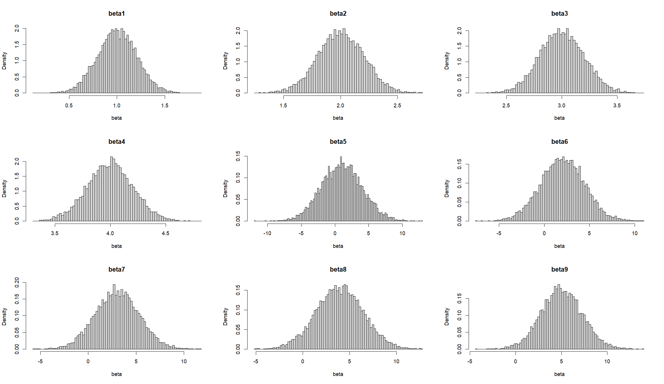
Figure 1: histogram of estimated $\hat{\beta}$ (no noise)

4.2 Model with noise

Suppose the noise matrix $E_{0}$ is a symmetric block diagonal matrix. Assume that $E_{0}$ is a block diagonal matrix, the matrices on its diagonal are symmetric, and the elements in the upper triangle of these matrices are i.i.d following $N(0,\sigma_{b}^{2})$. We take $\sigma_{b}=2^{-4},2^{-2},2^{-1},2^{0}$, $N=100$. The following are the outcomes of $n=10000$ experimental simulations:

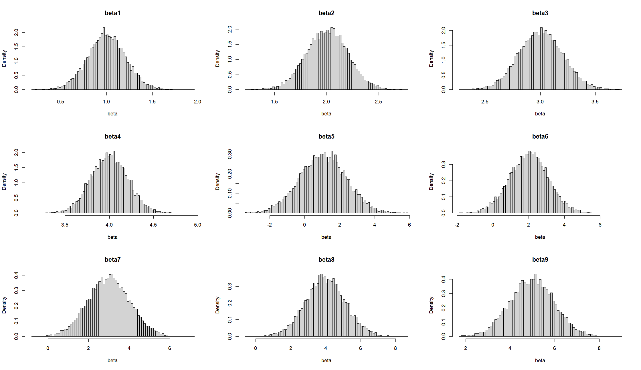
Figure 2: histogram of estimated $\hat{\beta}$ (with noise sd = $2^{-4}$, $N=100$)

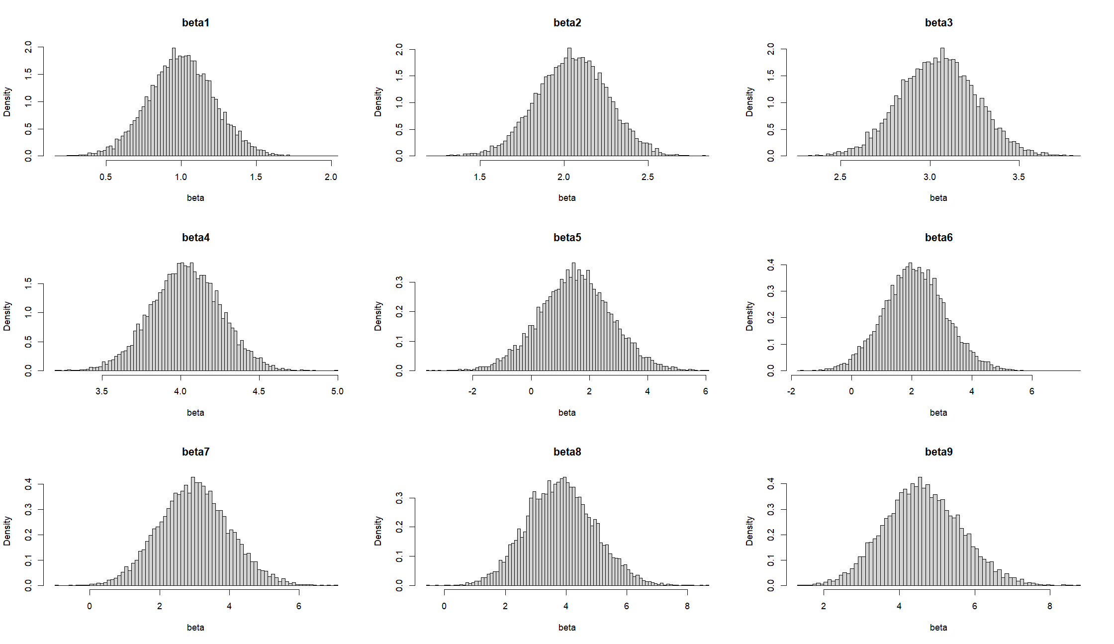
Figure 3: histogram of estimated $\hat{\beta}$ (with noise sd = $2^{-2}$, $N=100$)

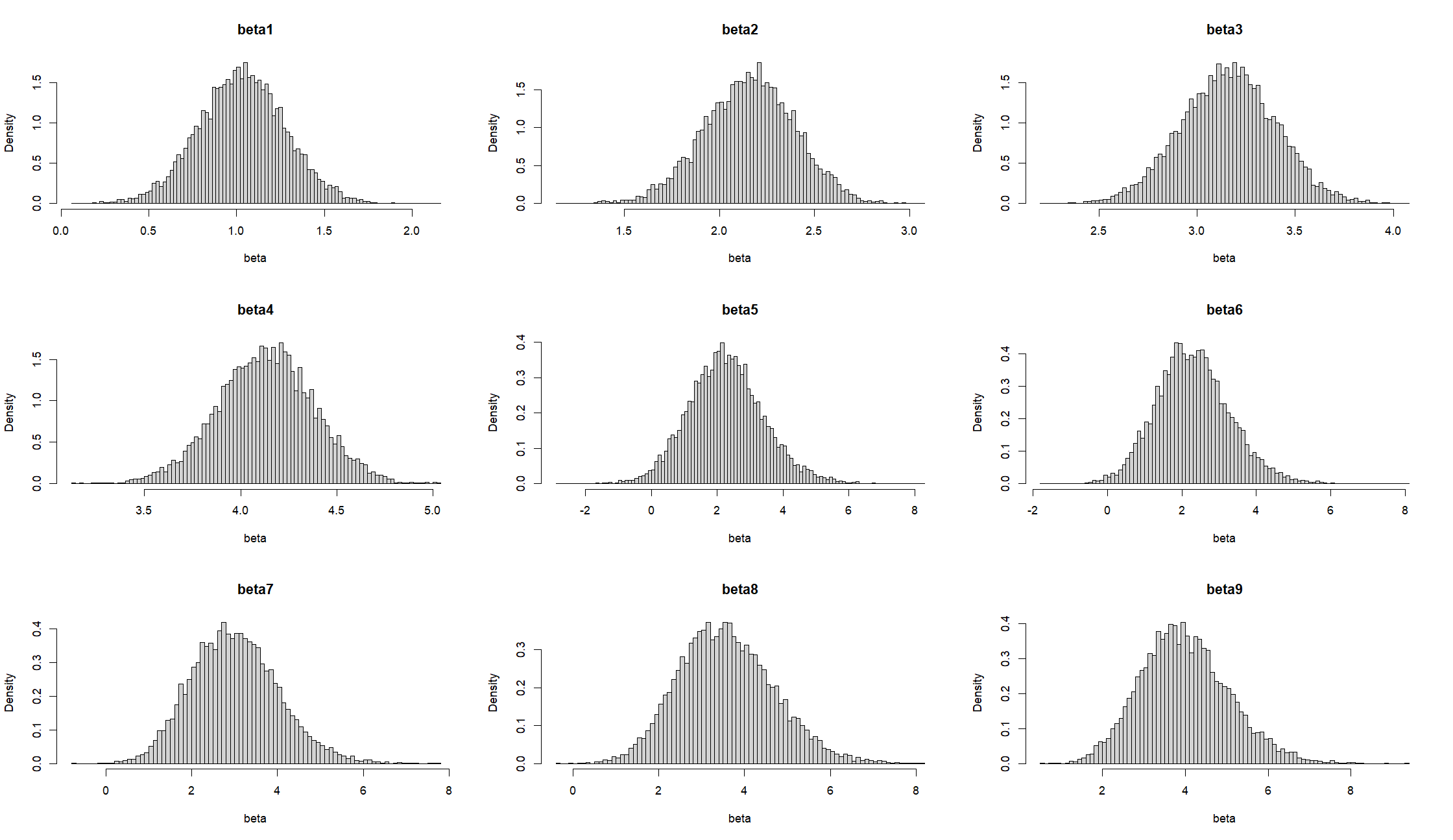
Figure 4: histogram of estimated $\hat{\beta}$ (with noise sd = $2^{-1}$, $N=100$)

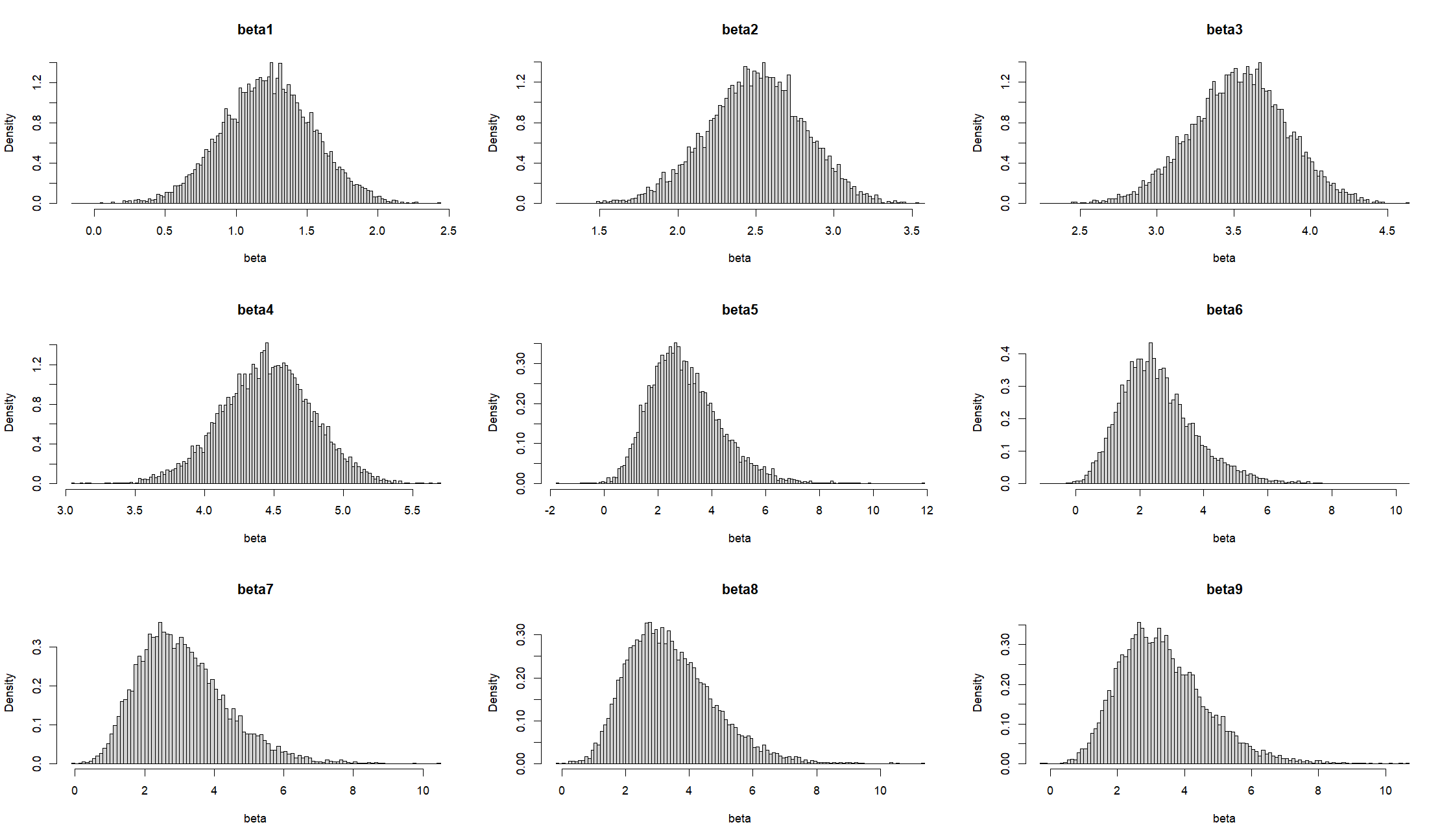
Figure 5: histogram of estimated $\hat{\beta}$ (with noise sd = $2^{0}$, $N=100$)

4.3 Model with community structure

In this section, we consider model (7) based on Random Interconnection Model in Chen and Hero (2018). (or Multi-layer stochastic block model in Holland et al. (1983)).

In the multi-graph SBM, networks are generated in the following manner. Suppose the size of communities $R=3$ and $\Pi=(\frac{1}{3},\frac{1}{3},\frac{1}{3})$ is the probability vector for a node to be assigned to each community. In our simulation, suppose the connection probability matrices $\mathcal{P}=\{P^{(1)},\cdots,P^{(L)}\}$ are identical and

$$P^{(\ell)}=\left[\begin{array}[]{ccc}0.8&0.1&0.1\\ 0.1&0.8&0.1\\ 0.1&0.1&0.8\end{array}\right].\ell=1,\cdots,L$$

Then the label of $N$ nodes is denoted as $Q=(c_{1},\cdots,c_{N})$. Here we take $\sigma_{b}=0.01$, $0.0625$, $0.125$, $0.25$, $0.5$, $1$ and $N=1000$. Suppose that $\beta_{X}=(1,2,3,4),\beta_{V}=(6,7,8,9,10),\beta_{Z}=5$, $\sigma_{y}=1$. The following are the outcomes of $n=1000$ experimental simulations:

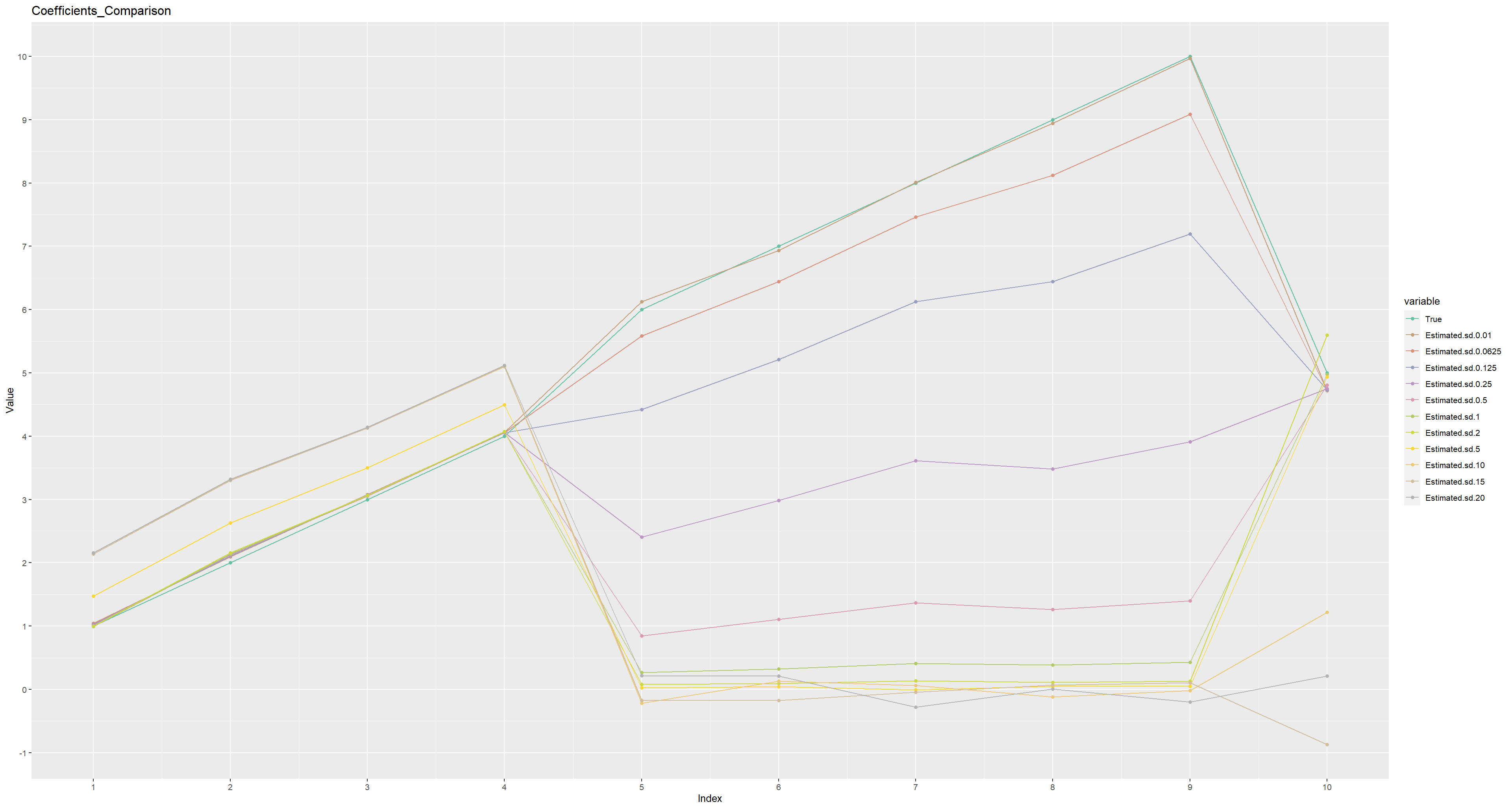
Figure 6: True vs estimated coefficients under different standard deviations

From the result above we found that the individual-component centrality coefficients are more sensitive (?probably) to the network noise compared to the community-component centrality coefficients.

5 Conclusion

By considering the community structure, our model is able to capture the effects of the underlying communities on the behavior of the network, thereby providing a more accurate and robust model for network analysis.

SUPPLEMENTARY MATERIAL

Proof of Theorem 2:

Let $\hat{W}=(X,\hat{C})$, then the two-stage estimator $\hat{\beta}$ turns out to be

$$\begin{array}[]{ll}\hat{\beta}&=(\hat{W}^{T}W)^{-1}\hat{W}^{T}y\\ &=\left(\begin{array}[]{cc}X^{T}X&X^{T}\hat{C}\\ \hat{C}^{T}X&\hat{C}^{T}\hat{C}\end{array}\right)^{-1}\left(\begin{array}[]{c}X^{T}\\ \hat{C}^{T}\end{array}\right)y\\ &=\left(\begin{array}[]{cc}(X^{T}(I_{N}-P_{\hat{C}})X)^{-1}&\boldsymbol{*}_{1}\\ \boldsymbol{*}_{2}&(\hat{C}^{T}(I_{N}-P_{X})\hat{C})^{-1}\end{array}\right)\end{array}$$ (12)

where

$$\begin{array}[]{ll}\boldsymbol{*}_{1}&=-(X^{T}(I_{N}-P_{\hat{C}})X)^{-1}X^{T}\hat{C}(\hat{C}^{T}\hat{C})^{-1}\\ &=-(X^{T}X)^{-1}X^{T}\hat{C}(\hat{C}^{T}(I_{N}-P_{X})\hat{C})^{-1},\end{array}$$ (13)

and

$$\begin{array}[]{ll}\boldsymbol{*}_{2}&=-(\hat{C}^{T}(I_{N}-P_{X})\hat{C})^{-1}\hat{C}^{T}X(X^{T}X)^{-1}\\ &=-(\hat{C}^{T}\hat{C})^{-1}\hat{C}^{T}X(X^{T}(I_{N}-P_{\hat{C}})X)^{-1}.\end{array}$$ (14)

Then

$$\hat{\beta}=\left(\begin{array}[]{c}\hat{\beta}_{X}\\ \hat{\beta}_{C}\end{array}\right)=\left(\begin{array}[]{c}(X^{T}(I_{N}-P_{\hat{C}})X)^{-1}X^{T}(I_{N}-P_{\hat{C}})y\\ (\hat{C}^{T}(I_{N}-P_{X})\hat{C})^{-1}\hat{C}^{T}(I_{N}-P_{X})y\end{array}\right).$$ (15)

Since $y=X\beta_{X}+C\beta_{C}+\varepsilon$, let $\delta_{C}=C-\hat{C}$, we have

$$\hat{\beta}=\left(\begin{array}[]{c}\hat{\beta}_{X}\\ \hat{\beta}_{C}\end{array}\right)=\beta+\left(\begin{array}[]{c}(X^{T}(I_{N}-P_{\hat{C}})X)^{-1}X^{T}(I_{N}-P_{\hat{C}})[\delta_{C}\beta_{C}+\varepsilon]\\ (\hat{C}^{T}(I_{N}-P_{X})\hat{C})^{-1}\hat{C}^{T}(I_{N}-P_{X})[\delta_{C}\beta_{C}+\varepsilon]\end{array}\right).$$ (16)

And from

$$(X^{T}(I_{N}-P_{\hat{C}})X)^{-1}X^{T}=(X^{T}X)^{-1}X^{T}(I_{N}+\hat{C}(\hat{C}^{T}(I_{N}-P_{X})\hat{C})^{-1}\hat{C}^{T}),$$ (17)

$$(\hat{C}^{T}(I_{N}-P_{X})\hat{C})^{-1}\hat{C}^{T}=(\hat{C}^{T}\hat{C})^{-1}\hat{C}^{T}(I_{N}+X(X^{T}(I_{N}-P_{\hat{C}})X)^{-1}X^{T}),$$ (18)

we have

$$\hat{\beta}=\left(\begin{array}[]{c}\hat{\beta}_{X}\\ \hat{\beta}_{C}\end{array}\right)=\beta+\left(\begin{array}[]{c}(X^{T}X)^{-1}X^{T}(I_{N}-P_{\hat{C}})[\delta_{C}\beta_{C}+\varepsilon]\\ (\hat{C}^{T}\hat{C})^{-1}\hat{C}^{T}(I_{N}-P_{X})[\delta_{C}\beta_{C}+\varepsilon]\end{array}\right)$$ (19)

In fact, $||\delta_{C}||_{F}=||C-\hat{C}||_{F}=||\tilde{u}_{1}-u_{1}||_{2}$. From Zhong (2017) we know that under assumption 3, $||\tilde{u}_{1}-u_{1}||_{2}=o_{P}(1)$, thus $||\delta_{C}||_{F}=o_{P}(1)$.

Now we consider the two blocks of difference between $\hat{\beta}$ and $\beta$ separately. For the first block, if $||\mathbb{E}[(I_{N}-P_{\hat{C}})\delta_{C}]||_{F}^{2}=0$, then $\mathbb{E}[(I_{N}-P_{\hat{C}})\delta_{C}]=0$.

$$\begin{array}[]{rl}||\mathbb{E}[(I_{N}-P_{\hat{C}})\delta_{C}]||_{F}^{2}&\leq\mathbb{E}[||(I_{N}-P_{\hat{C}})\delta_{C}||_{F}^{2}]\\ &=\text{tr}(\delta_{C}\delta_{C}^{T}(I-P_{\hat{C}}))\\ \text{(with Cauchy-Schwarz inequality) }&\leq(\text{tr}(\delta_{C}\delta_{c}^{T}\delta_{C}\delta_{C}^{T}))^{\frac{1}{2}}(\text{tr}(I_{N}-P_{\hat{C}}))^{\frac{1}{2}}\end{array}$$ (20)

Since $M:=\delta_{C}\delta_{C}^{T}$ is a real symmetric matrix, suppose $\mu_{i}$ are the eigenvalues of $M$, then

$$\sqrt{\text{tr}(M^{2})}=\sqrt{\sum\mu_{i}^{2}}\leq\sum_{i=1}^{N}|\mu_{i}|=\text{tr}(M).$$ (21)

We have

$$\mathbb{E}[||(I_{N}-P_{\hat{C}})\delta_{C}||_{F}^{2}]\leq\mathbb{E}[\text{tr}(M)\cdot(\text{tr}(I_{N}-P_{\hat{C}}))^{\frac{1}{2}}]$$ (22)

where

$$\text{tr}(I_{N}-P_{\hat{C}})=N-L$$ (23)

$$\text{tr}(M)=||C-\hat{C}||_{F}^{2}=||\tilde{u}_{1}-u_{1}||_{2}^{2}$$ (24)

Therefore,

$$\mathbb{E}[||(I_{N}-P_{\hat{C}})\delta_{C}||_{F}^{2}]\leq\sqrt{N-L}\cdot\mathbb{E}[\text{tr}(M)]=\sqrt{N-L}\cdot\mathbb{E}[||\tilde{u}_{1}-u_{1}||_{2}^{2}]$$ (25)

Under assumptions 1-3, we have $||\tilde{u}_{1}-u_{1}||_{2}=o_{P}(1)$. Therefore, we know $\tilde{u}_{1}-u_{1}=o_{P}(1)$, which means $\hat{C}-C=o_{P}(1)$. With the Slutsky’s Theorem and Continuous mapping theorem, we have

$$(X^{T}X)^{-1}X^{T}(I_{N}-P_{\hat{C}})\delta_{C}\stackrel{{\scriptstyle P}}{{\longrightarrow}}0$$ (26)

the estimator $\beta_{X}$ is weakly consistent.

For the second block, similarly, under assumptions 1-3, from $||\tilde{u}_{1}-u_{1}||_{2}=o_{P}(1)$ we know $\tilde{u}_{1}-u_{1}=o_{P}(1)$, which means $\hat{C}-C=o_{P}(1)$. With the Slutsky’s Theorem and Continuous mapping theorem, we have

$$(\hat{C}^{T}\hat{C})^{-1}\hat{C}^{T}(I_{N}-P_{X})\delta_{C}\stackrel{{\scriptstyle P}}{{\longrightarrow}}0$$ (27)

Thus the consistency of the second block is proved.

Denote

$$M=\left(\begin{array}[]{c}(X^{T}X)^{-1}X^{T}(I_{N}-P_{C})\\ (C^{T}C)^{-1}C^{T}(I_{N}-P_{X})\end{array}\right).$$ (28)

Then

$$\begin{array}[]{ll}\Sigma_{2}&=\sigma_{y}^{2}MM^{T}\\ &=\sigma_{y}^{2}\left(\begin{array}[]{cc}(X^{T}X)^{-1}X^{T}(I_{N}-P_{C})X(X^{T}X)^{-1}&0\\ 0&(C^{T}C)^{-1}C^{T}(I_{N}-P_{X})C(C^{T}C)^{-1}\end{array}\right).\end{array}$$ (29)

Proof of Theorem 3:

Similiar to the proof of Theorem 2, denote $\mathcal{X}=(X,Z)$, then the regression model in model (7) turns to $y=\mathcal{X}\beta_{\mathcal{X}}+V\beta_{V}+\varepsilon$. Denote $\hat{\mathcal{X}}=(X,\hat{Z})$, $\delta_{\mathcal{X}}=\mathcal{X}-\hat{\mathcal{X}}$, $\delta_{V}=V-\hat{V}$, then

$$\hat{\beta}=\left(\begin{array}[]{c}\hat{\beta}_{\mathcal{X}}\\ \hat{\beta}_{V}\end{array}\right)=\left(\begin{array}[]{c}(\hat{\mathcal{X}}^{T}(I_{N}-P_{\hat{Z}})\hat{\mathcal{X}})^{-1}\hat{\mathcal{X}}^{T}(I_{N}-P_{\hat{C}})y\\ (\hat{V}^{T}(I_{N}-P_{\hat{\mathcal{X}}})\hat{V})^{-1}\hat{V}^{T}(I_{N}-P_{\hat{\mathcal{X}}})y\end{array}\right).$$ (30)

From $y=\mathcal{X}\beta_{\mathcal{X}}+V\beta_{V}+\varepsilon$, we have

$$\hat{\beta}=\left(\begin{array}[]{c}\hat{\beta}_{\mathcal{X}}\\ \hat{\beta}_{V}\end{array}\right)=\beta+\left(\begin{array}[]{c}(\hat{\mathcal{X}}^{T}\hat{\mathcal{X}})^{-1}\hat{\mathcal{X}}^{T}(I_{N}-P_{\hat{V}})[\delta_{\mathcal{X}}\beta_{\mathcal{X}}+\delta_{V}\beta_{V}+\varepsilon]\\ (\hat{V}^{T}\hat{V})^{-1}\hat{V}^{T}(I_{N}-P_{\hat{\mathcal{X}}})[\delta_{\mathcal{X}}\beta_{\mathcal{X}}+\delta_{V}\beta_{V}+\varepsilon]\end{array}\right)$$ (31)

Further we know that $\delta_{\mathcal{X}}=\mathcal{X}-\hat{\mathcal{X}}=(X,Z)-(X,\hat{Z})=(0,\delta_{Z})$, $\delta_{\mathcal{X}}\beta_{\mathcal{X}}=\delta_{Z}\beta_{Z}$. Thus,

$$\hat{\beta}=\left(\begin{array}[]{c}\hat{\beta}_{\mathcal{X}}\\ \hat{\beta}_{V}\end{array}\right)=\beta+\left(\begin{array}[]{c}(\hat{\mathcal{X}}^{T}\hat{\mathcal{X}})^{-1}\hat{\mathcal{X}}^{T}(I_{N}-P_{\hat{V}})[\delta_{Z}\beta_{Z}+\delta_{V}\beta_{V}+\varepsilon]\\ (\hat{V}^{T}\hat{V})^{-1}\hat{V}^{T}(I_{N}-P_{\hat{\mathcal{X}}})[\delta_{Z}\beta_{Z}+\delta_{V}\beta_{V}+\varepsilon]\end{array}\right)$$ (32)

Similarly, under assumptions 1-4, we have $\hat{C}-C=o_{P}(1)$. From Lemma 2 and assumption 5, we have $\hat{S}-S=o_{P}(1)$. Thus with continuous mapping theorem, $\hat{U}-U=o_{P}(1)$, $\hat{Z}-Z=o_{P}(1)$, $\hat{\mathcal{X}}-\mathcal{X}=o_{P}(1)$, $\hat{V}-V=o_{P}(1)$. Therefore, $\delta_{Z}=o_{P}(1)$ and $\delta_{V}=o_{P}(1)$. Then

$$(\hat{\mathcal{X}}^{T}\hat{\mathcal{X}})^{-1}\hat{\mathcal{X}}^{T}(I_{N}-P_{\hat{V}})[\delta_{Z}\beta_{Z}+\delta_{V}\beta_{V}]\stackrel{{\scriptstyle P}}{{\longrightarrow}}0$$

and

$$(\hat{V}^{T}\hat{V})^{-1}\hat{V}^{T}(I_{N}-P_{\hat{\mathcal{X}}})[\delta_{Z}\beta_{Z}+\delta_{V}\beta_{V}]\stackrel{{\scriptstyle P}}{{\longrightarrow}}0.$$

Denote

$$\mathcal{M}=\left(\begin{array}[]{c}(\mathcal{X}^{T}\mathcal{X})^{-1}\mathcal{X}^{T}(I_{N}-P_{V})\\ (V^{T}V)^{-1}V^{T}(I_{N}-P_{\mathcal{X}})\end{array}\right).$$ (33)

Then

$$\begin{array}[]{ll}\Sigma_{3}&=\sigma_{y}^{2}\mathcal{M}\mathcal{M}^{T}\\ &=\sigma_{y}^{2}\left(\begin{array}[]{cc}(\mathcal{X}^{T}\mathcal{X})^{-1}\mathcal{X}^{T}(I_{N}-P_{V})\mathcal{X}(\mathcal{X}^{T}\mathcal{X})^{-1}&0\\ 0&(V^{T}V)^{-1}V^{T}(I_{N}-P_{\mathcal{X}})V(V^{T}V)^{-1}\end{array}\right).\end{array}$$ (34)

References

- Allen et al. (2019) Allen, F., J. Cai, X. Gu, J. Qian, L. Zhao, W. Zhu, et al. (2019). Ownership networks and firm growth: What do forty million companies tell us about the chinese economy? Available at SSRN 3465126.
- Banerjee et al. (2019) Banerjee, A., A. G. Chandrasekhar, E. Duflo, and M. O. Jackson (2019). Using gossips to spread information: Theory and evidence from two randomized controlled trials. The Review of Economic Studies 86(6), 2453–2490.
- Benson (2019) Benson, A. R. (2019). Three hypergraph eigenvector centralities. SIAM Journal on Mathematics of Data Science 1(2), 293–312.
- Cai et al. (2021) Cai, J., D. Yang, W. Zhu, H. Shen, and L. Zhao (2021). Network regression and supervised centrality estimation. arXiv preprint arXiv:2111.12921.
- Chen and Hero (2018) Chen, P.-Y. and A. O. Hero (2018). Phase transitions and a model order selection criterion for spectral graph clustering. IEEE Transactions on Signal Processing 66(13), 3407–3420.
- De Domenico et al. (2013) De Domenico, M., A. Solé-Ribalta, E. Cozzo, M. Kivelä, Y. Moreno, M. A. Porter, S. Gómez, and A. Arenas (2013). Mathematical formulation of multilayer networks. Physical Review X 3(4), 041022.
- De Domenico et al. (2013) De Domenico, M., A. Solé-Ribalta, E. Omodei, S. Gómez, and A. Arenas (2013). Centrality in interconnected multilayer networks. arXiv preprint arXiv:1311.2906.
- De Domenico et al. (2015) De Domenico, M., A. Solé-Ribalta, E. Omodei, S. Gómez, and A. Arenas (2015). Ranking in interconnected multilayer networks reveals versatile nodes. Nature communications 6(1), 6868.
- Han et al. (2015) Han, Q., K. Xu, and E. Airoldi (2015). Consistent estimation of dynamic and multi-layer block models. In International Conference on Machine Learning, pp. 1511–1520. PMLR.
- Holland et al. (1983) Holland, P. W., K. B. Laskey, and S. Leinhardt (1983). Stochastic blockmodels: First steps. Social networks 5(2), 109–137.
- Jackson et al. (2008) Jackson, M. O. et al. (2008). Social and economic networks, Volume 3. Princeton university press Princeton.
- Kolaczyk and Csárdi (2014) Kolaczyk, E. D. and G. Csárdi (2014). Statistical analysis of network data with R, Volume 65. Springer.
- Lin et al. (2022) Lin, W., L. Xu, and H. Fang (2022). Finding influential edges in multilayer networks: Perspective from multilayer diffusion model. Chaos: An Interdisciplinary Journal of Nonlinear Science 32(10).
- Liu and Zhao (2023) Liu, X. and C. Zhao (2023). Eigenvector centrality in simplicial complexes of hypergraphs. Chaos: An Interdisciplinary Journal of Nonlinear Science 33(9).
- Newman (2013) Newman, M. E. (2013). Spectral methods for community detection and graph partitioning. Physical Review E 88(4), 042822.
- Newman and Girvan (2004) Newman, M. E. and M. Girvan (2004). Finding and evaluating community structure in networks. Physical review E 69(2), 026113.
- Palla et al. (2005) Palla, G., I. Derényi, I. Farkas, and T. Vicsek (2005). Uncovering the overlapping community structure of complex networks in nature and society. nature 435(7043), 814–818.
- Pothen (1997) Pothen, A. (1997). Graph partitioning algorithms with applications to scientific computing. In Parallel Numerical Algorithms, pp. 323–368. Springer.
- Richmond (2019) Richmond, R. J. (2019). Trade network centrality and currency risk premia. The Journal of Finance 74(3), 1315–1361.
- Rowlinson (1996) Rowlinson, P. (1996). D. m. cvetković, m. doob and h. sachs spectra of graphs (3rd edition) (johann ambrosius barth verlag, heidelberg-leipzig 1995), 447 pp., 3 335 00407 8, dm 168. Proceedings of the Edinburgh Mathematical Society 39(1), 188–189.
- Solá et al. (2013) Solá, L., M. Romance, R. Criado, J. Flores, A. García del Amo, and S. Boccaletti (2013). Eigenvector centrality of nodes in multiplex networks. Chaos: An Interdisciplinary Journal of Nonlinear Science 23(3).
- Tudisco et al. (2018) Tudisco, F., F. Arrigo, and A. Gautier (2018). Node and layer eigenvector centralities for multiplex networks. SIAM Journal on Applied Mathematics 78(2), 853–876.
- White and Smyth (2005) White, S. and P. Smyth (2005). A spectral approach to finding communities in graphs. In Proc. SIAM Conf. on Data Mining.
- Wu et al. (2019) Wu, M., S. He, Y. Zhang, J. Chen, Y. Sun, Y.-Y. Liu, J. Zhang, and H. V. Poor (2019). A tensor-based framework for studying eigenvector multicentrality in multilayer networks. Proceedings of the National Academy of Sciences 116(31), 15407–15413.
- Zhong (2017) Zhong, Y. (2017). Eigenvector under random perturbation: A nonasymptotic rayleigh-schrödinger theory. arXiv preprint arXiv:1702.00139.