Universality of Anderson Localization Transitions in the Integer and Fractional Quantum Hall Regime

Abstract

Understanding the interplay between electronic interactions and disorder-induced localization has been a longstanding quest in the physics of quantum materials. One of the most convincing demonstrations of the scaling theory of localization for noninteracting electrons has come from plateau transitions in the integer quantum Hall effect [1] with short-range disorder [2], wherein the localization length diverges as the critical filling factor is approached with a measured scaling exponent close to the theoretical estimates [3]. In this work, we extend this physics to the fractional quantum Hall effect [4], a paradigmatic phenomenon arising from a confluence of interaction, disorder, and topology. We employ high mobility trilayer graphene devices where the transport is dominated by short-range impurity scattering, and the extent of Landau level mixing can be varied by a perpendicular electric field [5, 6]. Our principal finding is that the plateau-to-plateau transitions from $N+1/3$ to $N+2/5$ and from $N+2/5$ to $N+3/7$ fractional states are governed by a universal scaling exponent, which is identical to that for the integer plateau transitions and is independent of the perpendicular electric field. These observations and the values of the critical filling factors are consistent with a description in terms of Anderson localization-delocalization transitions [7] of weakly interacting electron-flux bound states called composite Fermions [8, 9, 10]. This points to a universal effective physics underlying fractional and integer plateau-to-plateau transitions independent of the quasiparticle statistics of the phases and unaffected by weak Landau level mixing. Besides clarifying the conditions for the realization of the scaling regime for composite fermions, the work opens the possibility of exploring a wide variety of plateau transitions realized in graphene, including the fractional anomalous Hall phases [11] and non-abelian FQH states [12].

The Quantum Hall (QH) effect realizes multiple continuous phase transitions between distinct insulating topological states (separated by delocalized states) in a two-dimensional electron gas subject to a perpendicular magnetic field [1]. The magnetic field $B$ quantizes the electronic kinetic energy into discrete Landau energy levels (LL). Disorder localizes all electronic single-particle states in the bulk of the material, barring those at a specific critical energy $E_{c}$ situated near the center of each disorder-broadened LL. The states at $E_{c}$ are extended [13, 14, 15, 16, 17, 18]. When the Fermi energy lies between the extended states of the $N^{\rm th}$ and the $(N+1)^{\rm st}$ LLs, the system is in a topological phase. The electrical transport is characterized by a plateau in the transverse resistance quantized to $R_{xy}=h/(Ne^{2})$ accompanied by a vanishingly small longitudinal resistance $R_{xx}\approx 0$. This is the integer quantum Hall (IQH) regime. As the Fermi energy approaches $E_{c}$, the localization length $\xi$ characterizing the single-particle states diverges as $\xi\propto|E-E_{c}|^{-\gamma}$ (in practice, this divergence is cut-off by the effective sample size or temperature). This, in turn, leads to a peak in $R_{xx}$ that accompanies the transition between two successive $R_{xy}$ plateaus [3, 18, 19, 20]. The physics in such a critical regime results in several unusual phenomena, such as anomalous diffusion [21], multifractal local density of states [7, 22], and multifractal conductance fluctuations [23, 24].

Low temperatures and high magnetic fields enhance the effective electron-electron interaction, producing a richer set of the fractional quantum Hall (FQH) phases [25]. Two paradigmatic perspectives are in place. First, FQH physics is marked by strong many-body correlations characteristic to each incompressible phase, with the FQH plateau transitions arising from changes to the characteristic correlations. This strongly interacting picture may suggest that the critical behavior at the transitions between FQH phases differs markedly from the analogous transitions in the IQH regime. Second, the FQH transitions can be associated with integer quantum Hall physics by implementing the composite Fermion (CF) approximation, whereby FQH phases are described as integer quantum Hall phases of weakly interacting CFs. These composite particles are formed by attaching an even number of flux quanta to electrons [26]. This results in a one-to-one correspondence between the low energy physics of the IQH and FQH phases (the so-called law of corresponding states for CFs [27, 9]) and further predicts the Anderson localization in the FQH regime to be analogous to that in the IQH regime [8, 27, 26], with both phases characterized by the same set of universal critical exponents  [10, 28]. Experimentally deducing the near-critical-point scaling is highly desirable in elucidating the inter-FQH-plateau critical behavior when facing these two paradigmatic pictures.

To experimentally determine $\gamma$, the finite-size scaling theory suggests examining the divergence (with respect to temperature $T$) of the quantity d$R_{xy}/$d$\nu$ versus the Landau level filling factor $\nu$ measured at the critical point $\nu=\nu_{c}$ (corresponding to critical energy $E_{c}$) [20, 29]:

$$(dR_{xy}/d\nu)_{\nu=\nu_{c}}\propto T^{-\kappa}.$$ (1)

Here, $\nu=nh/eB$, $B$ is the magnetic field, $n$ is the areal charge-carrier density, $h$ is the Planck constant, and $e$ is the electronic charge. The scaling exponent $\kappa$ and the localization length exponent $\gamma$ are related by $\kappa=p/2\gamma$ [30, 3, 20], where $p$ determines the power-law divergence of the phase coherence length $L_{\phi}$ with temperature: $L_{\phi}\propto T^{-p/2}$. Their values are predicted to be $\gamma\approx 2.3$ and $\kappa\approx 0.42$ for all IQH and FQH transitions [9, 20, 29, 15, 31].

Experimental investigations of scaling in the IQH regime have reported $\kappa$ varying between $0.16\leq\kappa\leq 0.81$ (Supplementary Information, Section S8). This wide variation has been attributed to varying disorder correlation lengths with a universal critical behavior seen only in samples with short-range disorder [32, 33]. Similar experimental investigations of scaling laws at transitions between FQH phases are scarce [34, 35, 36]. A recent experimental study on extremely high-mobility 2D electron gas confined to GaAs quantum wells found the value of $\kappa$ in the FQH regime to be non-universal, this observation being attributable to long-range disorder correlation [36].

These recent studies [36, 9, 10] motivated us to experimentally revisit the scaling of FQH transitions in a platform where the nature of disorder scattering can be controlled. We leverage the fact that the electrical transport properties of high-mobility graphene devices are dominated by short-range impurity scattering, noting that those of low-mobility graphene devices are controlled by both short-ranged and long-ranged scattering potentials [37]. Thus, high-mobility graphene devices represent a natural candidate to investigate the universality of scaling exponents. Choosing Bernal-stacked trilayer graphene (TLG) as our system of study allows the additional flexibility to probe the effect of band-mixing on the scaling properties of IQH and FQH states by tuning the Landau level spectra using an external displacement field $D$ [6, 5, 38]. The $D$-field breaks the mirror reflection symmetry of the lattice, and the resulting hybridization of the monolayer-like and bilayer-like bands can lead to changes in interaction strength and symmetries in the QH phases [6] and the emergence of degenerate groups of LLs [5]. Choosing Bernal-stacked trilayer graphene (TLG) as our system of study allows the additional flexibility to probe the effect of band-mixing on the scaling properties of IQH and FQH states.

This Article experimentally validates the universal scaling law governing IQH and FQH transitions. We extract the values of $\kappa$ near criticality, $\nu=\nu_{c}$, using three distinct approaches: (i) analyzing the critical divergence of $dR_{xy}/d\nu$, (ii) probing the critical divergence of the inverse of the width of $R_{xx}$, and (iii) performing a scaling analysis of $R_{xy}$ near the critical point. The results consistently show that for all IQH and FQH plateau-to-plateau transitions (PT), closely aligned with the predictions of the scaling theory [3].

Our study provides the first definite evidence of the Anderson localization in the FQH regime. The stability of the critical exponents as the perpendicular displacement field is varied suggests that weak Landau level mixing does not perturb the values of these critical exponents. Comparison between graphene devices of varying mobility shows that as long as long-range impurity scattering can be suppressed, the universality of scaling parameters perseveres, independent of the quantum Hall bulk phases involved. In this limit, the universality found underscores the applicability of the CF approximation.

Results

Standard dry transfer technique is used for the fabrication of dual graphite-gated hexagonal-boron-nitride (hBN) encapsulated TLG devices [Fig. 1(a)] (for details, see Supplementary Information, section S1) [39]. Fig. 1(b) shows measurements of the longitudinal resistance $R_{xx}$ and the transverse conductance $G_{xy}$ versus the Landau level filling factor $\nu$; the measurements were performed at $B=13$ T, $T=20$ mK and $D=0$ V/nm. We identify several major odd denominator FQH states ($\nu=1/3,2/5,3/7$ and their hole-conjugates) by prominent dips in $R_{xx}$ and corresponding plateaus in $G_{xy}$; this is the first observation of these relatively well-developed FQH states in TLG. Although ill-formed, indications of $\nu=n+1/5$ and $n+2/7$ states are also seen. Several of these FQH states are resolved at $B=4.5$ T, attesting to the high quality of the device in terms of excellent homogeneity of number density and suppression of long-range scattering (Supplementary Information, Section S6).

The band structure of TLG for $D=0$ V/nm is formed of monolayer-like and bilayer-like Landau levels (Fig. 1(c)) – these are protected from mixing by the lattice mirror-symmetry [40]. The calculated LLs as a function of $B$ and energy $E$ are shown in Fig. 1(d), where blue (red) lines mark the LLs originating from the monolayer-like (bilayer-like) LLs. The $N_{M}=0$ monolayer-like LLs cross the bilayer-like LLs at $B\approx 6$ T. For $B>8$ T, the $\nu=2$ and $\nu=3$ arise from the spin-split $N_{M}=0^{-}\uparrow$ and $N_{M}=0^{-}\downarrow$ bands of the monolayer-like LLs. Here, $(+,-)$ refer to the two valleys and $(\uparrow,\downarrow)$ refer to electronic spins. We confine our study to $8$ T$<B<10$ T to avoid Landau level-mixing at lower–$B$ and phase transitions between competing FQH states at higher–$B$ [41, 42, 43].

Critical exponents near FQH plateau-to-plateau transitions

Fig. 2(a) shows the $T$-dependence of $R_{xy}$ between the IQH states $\nu=-2$ and $\nu=-1$. Similar data for transition between the FQH states $\nu=2+2/3$ and $\nu=2+3/5$ are shown in Fig. 2(b). The critical points $\nu_{c}$ of the plateau-to-plateau transition (identified as the crossing point of the $R_{xy}$ curves at different $T$) are indicated in the plots. The exponent $\kappa$ evaluated from the peak value of d$R_{xy}$/d$\nu$ versus $T$ near criticality (Figs. 2(c-d)) using Eqn. 1 in both cases is $\kappa=0.41\pm 0.01$. Analysis of the $T$-dependence of the inverse of the half-width of $R_{xx}$ as $\nu$ is varied between two consecutive FQH plateaus also yield $\kappa=0.41\pm 0.02$ (Supplementary Information, section S2).

Having extracted $\kappa$ from power-law fits, we now demonstrate the scaling properties of $R_{xy}$ in the vicinity of $\nu_{c}$. We use the following form [3]:

$$R_{xy}(\nu,T)=R_{xy}(\nu_{c})f[\alpha(\nu-\nu_{c})]$$ (2)

with

$$\alpha\propto T^{-1/(z\gamma)}$$ (3)

Here, $z$ is the dynamical critical exponent characterizing the critical slowing down near a phase transition [44, 2], $f(0)=1$, and $f^{\prime}(0)\neq 0$. From Eq. 2 and Eq. 3, it follows that $dR_{xy}/d\nu_{\nu=\nu_{c}}\propto T^{-1/(z\gamma)}$. A comparison of this expression with Eq. 1 gives $\kappa=1/(z\gamma)$ [3]. This gives us a second, independent method of estimating $\kappa$. Figure 2(e) shows $R_{xy}/R_{xy}(\nu_{c})$ at various temperatures as a function of $\alpha|\nu-\nu_{c}|$ for the $\nu=2+1/3$ to $2+2/5$ transition. $\alpha(T)$ is optimized to collapse the various constant-temperature data onto a single curve (the upper branch of which is for $\nu<\nu_{c}$, and the lower branch is for $\nu>\nu_{c}$). From the plot of $\alpha$ versus $T$ (inset of Fig. 2(e)) we obtain $\kappa=0.40\pm 0.03$.

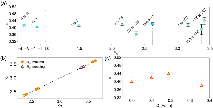
Figure 3: Scaling exponents for different PT (a) Plot of $\kappa$ as a function of $\nu_{c}$ corresponding to different PT. The dotted vertical lines mark the experimentally obtained $\nu_{C}$. (b) Plot of experimentally obtained values of critical points, $\nu_{c}$ versus those theoretically calculated $\nu_{ct}$  [9]. The triangles are the values determined from crossing points of isotherms in $R_{xy}$ while the circles are determined from the $R_{xx}$ maxima. The black dashed line fits the data points with slope = $1.00\pm 0.002$ (c) Plot of $\kappa$ versus $D$ for the FQH transition from $\nu=8/3$ to $\nu=13/5$ states.

Fig. 3(a) compiles our findings. These results indicate a $\kappa$ value of $0.41\pm 0.03$ uniformly observed across all probed transitions between IQH and FQH states (compare with Fig. S8 of Supplementary Information). This consistency in scaling spans various transition types, including transitions from one IQH state to another, transitions among different FQH states, and transitions between an IQH state and a neighboring FQH state. Such consistency underscores the universal applicability of this scaling principle. This universality of $\kappa$ using three independent methods marks the first experimental confirmation of a uniform scaling law across FQH transitions in any material. It is the central result of this Article.

The physics of the FQH effect of electrons at a filling factor $\nu$ can be mapped onto that of IQH of CF at a filling factor $\nu_{CF}$, with $\nu=\nu_{CF}/(2\nu_{CF}\pm 1)$ [26]. It follows that the critical points for the FQH PT occur at [9, 45]:

$$\nu_{c}=\frac{(\nu_{CF}+0.5)}{2(\nu_{CF}+0.5)\mp 1}.$$ (4)

The experimentally obtained values of $\nu_{c}$, extracted either from the crossing point of the $R_{xy}$ isotherms or the maxima of $R_{xx}$, match exceptionally well with the theoretical predictions (Fig. 3(b)) (Supplementary Information, table S1). To our knowledge, this is the first experimental verification of the Eqn. 4, which relates the critical points for FQH of electrons with those of IQH of CF. Furthermore, it seems to validates the employment of a weakly interacting CF picture even far away from the center of the plateaus  [9].

Robustness of the critical exponents against LL mixing. A non-zero vertical displacement field $D$ gives rise to a complex phase diagram in TLG, with the Landau levels inter-crossing multiple times, resulting in significant LL mixing as either $D$ or $B$ is varied [46, 47, 48, 5, 49]. LL-mixing can change the effective interaction between the electrons [43]; however, as shown in Fig. 3(c), we find that it does not affect the universality of $\kappa$ significantly. This vital result suggests that as long as the CFs are weakly interacting (as indicated by the presence of the Jain sequence of states), the critical behavior of the localization-delocalization transition remains unaltered.

Discussion

We are now in a position to compare the universality of $\kappa$ seen in the FQH PT in our high-mobility TLG with non-universality of the same measured in the high-mobility 2D electronic gas confined to GaAs quantum wells [36]. The large spread in $\kappa$ values seen in the data in GaAs quantum wells can be attributed to two main reasons [36]. The first is the formation of numerous developing FQH phases between $\nu=1/3$ and $2/5$, which limits the temperature range over which one observes the decrease of $\Delta$ with $T$ ($\Delta$ being the width of $R_{xx}$). Note that in Fig. 1(b), there are two incipient FQH phases, $\nu=3+1/5$ and $3+2/7$ visible in the $R_{xx}$ trace, between the more robust phases $\nu=3$ and $\nu=3+1/3$. The incipient phases are weak enough to not affect the scaling of the transition region in $R_{xy}$ even at the lowest temperature employed here. As a result, we find $\kappa=0.42\pm 0.01$ (Fig. 3(a)).

The second reason for the deviation of the scaling exponent from $0.42$ in GaAs quantum wells is related to the type of disorder present in the sample [36]. Universality in $\kappa$ is observed only when effective disorder potential is short-ranged [33] (as in our graphite-gated high-mobility graphene devices) whereas, in GaAs/AlGaAs systems, long-range interaction from the impurities leads to long-range disorder potential fluctuations [36]. We fabricated graphene devices without the graphite gate electrodes to probe the effect of long-range interactions on $\kappa$. The graphene channel was no longer screened from long-range Coulomb fluctuations arising from the SiO2 substrate. In these devices, the value of $\kappa$ varied widely between $0.45-0.64$ (Supplementary Information, section S4), supporting the conclusions of Ref [36].

To summarize, the critical behavior associated with transitions between FQH plateaus is underlined by strongly correlated, strongly interacting phases of electronic matter. It is not immediately evident that the scaling involved should match the scaling behavior in IQH transitions. Our universal scaling, effective to transitions between Abelian FQH states and identical to the scaling found for IQH phases, validates the Composite Fermion approximation. Specifically, we have demonstrated the scaling of the conductance (with a scaling exponent $\kappa=0.41\pm 0.02$) in the IQH and FQH states in Bernal-stacked ABA trilayer graphene. This scaling holds for all plateau-to-plateau transitions between two consecutive IQH states, between two FQH states, and even between IQH and the adjoining FQH state, underlining the universal character of the scaling. To our knowledge, ours is the first definite observation of Anderson localization-delocalization transition over a series of fractional QH states.

Furthermore, we observe the universality of $\kappa$ (both in IQH and FQH regimes) even when an external displacement field hybridizes the Landau levels of Bernal-stacked TLG. We find deviations from universality in the value of $\kappa$ only in devices where long-range scattering dominates, in agreement with Ref. [36]. Further theoretical studies are required to understand the observed similarities between the transitions in integer and fractional quantum Hall states, to explore the validity of the weakly interacting CF description in the plateau transition regions, and to develop effective descriptions of the role of disorder on anyonic matter. Our study raises the question of whether the universality observed in this context applies to transitions between closely related bulk phases, such as fractional Chern insulators [11], and phases potentially characterized by non-Abelian topological order [50, 51, 52] that go beyond the conventional CF description.

Methods

Device fabrication and measurement

Device of dual graphite gated ABA trilayer graphene (TLG) heterostructures were fabricated using a dry transfer technique (for details, see Supplementary materials S1). Raman spectroscopy and optical contrast were used to determine the number of layers and stacking sequence. The devices were patterned using electron beam lithography, followed by reactive ion etching and thermal deposition of Cr/Pd/Au contacts. Measurements were done in a cryogen-free refrigerator (with a base temperature of $\mathrm{20~{}mK}$) at low frequency using standard low-frequency measurement techniques. Dual electrostatic gates were used to simultaneously tune the areal number density $n=[(C_{tgVtg}+C_{bgVbg})/e+n_{o}]$ and the displacement field $D=[(C_{bg}V_{bg}-C_{tg}V_{tg})/2\epsilon_{o}+D_{o}]$ across the device. Here $C_{bg}(C_{tg})$ is the back gate (top gate) capacitance, and $V_{bg}(V_{tg})$ is the back gate (top gate) voltage. The values of $C_{tg}$ and $C_{bg}$ are determined from quantum Hall measurements. $n_{o}$ and $D_{o}$ are the residual number density and electric field due to unavoidable impurities in the channel.

Data availability

The authors declare that the data supporting the findings of this study are available within the main text and its Supplementary Information. Other relevant data are available from the corresponding author upon reasonable request.

Author contributions

S.K., T.C., K.R.A., and A.B. conceived the idea of the study, conducted the measurements, and analyzed the results. T.T. and K.W. provided the hBN crystals. U.G., G.J.S., and Y.G. developed the theoretical model. All the authors contributed to preparing the manuscript.

^† These authors contributed equally.

Competing interests

The authors declare no competing interests.

Figure 1: FQH in Bernal-stacked TLG (a) Device schematics of TLG encapsulated between two hBN and few-layer graphite flakes. (b) Line plots of $G_{xy}$ (left-axis; solid green line) and $R_{xx}$ (right-axis; solid blue line) versus $\nu$ measured at $B=13$ T, $T=20$ mK, and $D=0$ V/nm. The dashed vertical lines mark the FQH states formed at corresponding $\nu$, and the arrows indicate corresponding plateaus in $G_{xy}$ (c) Calculated band structure of Bernal stacked trilayer graphene for $D=0$ V/nm. The four LLs of the $N_{M}=0$ band are indicated schematically. (d) Calculated Landau levels as a function of energy $E$ and $B$ for $D=0$ V/nm. The blue lines are the monolayer-like LLs, while the red lines are the bilayer-like LLs. The solid and dotted lines indicate the LLs from $K$ and $K^{\prime}$-valley, respectively. The solid-green line is the spin-degenerate $N_{M}=0^{-}\uparrow$ and $N_{M}=0^{-}\downarrow$ monolayer-like LLs that host the FQH states probed in this Article.

Figure 2: Scaling near $\nu=\nu_{c}$. Plot of $R_{xy}$ versus $\nu$ for transition between the (a) IQH states $\nu=-2$ and $\nu=-1$ (the critical point $\nu_{c}=-1.51$), and (b) the FQH states $2+2/3$ and $2+3/5$ ($\nu_{c}=2.625$). (c) Log-log plot of $|\mathrm{d}R_{xy}/\mathrm{d}\nu|$ versus $T$ for the PT $\nu=-2$ and $\nu=-1$ at $\nu_{c}$. The dashed line is the fit to the data points using Eqn. 1. (d) Same as in (c) for the PT between FQH states $2+2/3$ and $2+3/5$. (e) Scaling analysis of $R_{xy}$ for the PT transition between $\nu=2+1/3$ and $\nu=2+2/5$. The inset is a plot of $T$ versus $\alpha$ in a log-log scale (open circles); a linear fit to the data (dotted line) yields $\kappa=0.40\pm 0.03$. (For an error analysis, see Supplementary Information Section S7.)

Supplementary Information

S1 Device fabrication, schematics and characterization

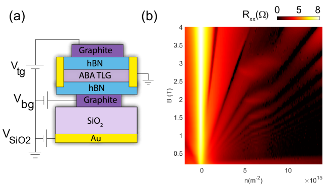
Figure S1: (a) Schematic of the device. Two gates $V_{bg}$ and $V_{tg}$ (with 30 nm thick hBN flakes as gate dielectrics and thin graphite as gate contacts) are used to tune the number density and displacement field across the flake. A silicon back-gate (with SiO2 as the gate dielectric) is used to dope the graphene contacts of the device to prevent the formation of p-n junctions. (b) Landau level fan diagram for TLG measured at $7$ K. Color map shows the $R_{xx}$ in log scale.

Bernal-stacked trilayer graphene (TLG), hBN, and graphite flakes are mechanically exfoliated on Si substrates with a 300 nm thick top SiO₂ layer. TLG flakes are first identified through color contrast under an optical microscope and further confirmed using Raman spectroscopy [53, 54]. The standard dry pickup and transfer technique is used to fabricate the heterostructure. The flakes are picked up sequentially using polycarbonate (PC) film at $T=120^{\circ}$ C in the following order: graphite/hBN/TLG/hBN/graphite. The entire stack, along with the PC film, is transferred on Si/SiO2 substrate at $180^{\circ}$ C followed by cleaning in chloroform, acetone, and IPA solution to remove the PC residue. The heterostructure is then annealed in vacuum at $300^{\circ}$ C for $4$ hours. We employ electron beam lithography for defining the contacts on the heterostructure. This is followed by etching with a mixture of CHF3 and O2 gases and metal deposition with Cr/Pd/Au ($3$ nm/$12$ nm/$55$ nm) to create 1-D contacts [55, 56].

Avoiding the formation of p-n junctions is absolutely essential if the devices are to be operated at high displacement fields [57, 49, 58]. We achieve this by doping the graphene contacts (that extend out of both the graphite gates) to high number density. A schematic of the device is shown in Fig. S1(a). Two common kinds of TLG flakes are typically obtained during mechanical exfoliation: ABA (or Bernal-stacked) and ABC. ABC, being a metastable stacking [59, 60], generally converts into ABA stacking during fabrication. These two phases are easily distinguishable by Raman spectroscopy and transport measurements – displacement field opens up a band gap in ABC TLG  [61, 62, 63]. In contrast, a band gap does not open in ABA TLG.

Fig. S1(b) shows the Landau level fan diagram of the sample measured at 7 K. It matches pretty well with the simulated LL plot shown in Fig. 1(d) of the main manuscript with clear indications of monolayer-like Landau levels (LL) around a number density $5\times 10^{15}$ $\mathrm{m^{-2}}$ that cross the bilayer-like LLs confirming the system to be ABA trilayer graphene [38, 64].

S2 Estimation of $\kappa$ from the temperature dependence of the width of $R_{xx}$.

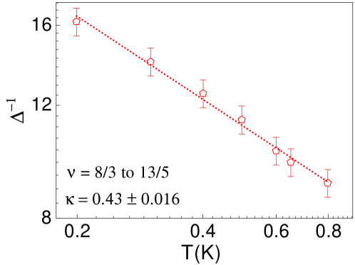
Figure S2: Calculating $\kappa$ from width of $R_{xx}$. Log-log plots of the inverse of the half-width of longitudinal magnetoresistance $R_{xx}$ versus $T$ for PT between $\nu=2+2/3$ and $\nu=2+3/5$.

At the critical point of the quantum Hall plateau-to-plateau transitions (PT), both d$R_{xy}$/d$\nu$ and the inverse of the half-width of $R_{xx}$ versus $\nu$ plot diverge according to power law $T^{-\kappa}$ [3]. In the main manuscript, we estimated the value of $\kappa$ by evaluating d$R_{xy}$/d$\nu$ close to the critical point. Here, we focus on the analysis of the width $\Delta$ of $R_{xx}$ (FWHM of $R_{xx}$ transition peak) versus $\nu$ [30, 34]. At the critical point, $\Delta^{-1}$ diverges like $T^{-\kappa}$. The dependence of $\Delta^{-1}$ on $T$ for the transition between $\nu=2+2/3$ and $\nu=2+3/5$ is shown in Fig. S2. The slope of linear fits to data yields $\kappa=0.43\pm 0.016$.

S3 Critical behavior of plateau-to-plateau transitions

In table S1, we compare our experimentally obtained values of $\nu_{c}$ with the theoretically predicted values [65, 9]:

$$\nu_{c}=\frac{(n+0.5)}{2\hskip 2.84526pt(n+0.5)\pm 1};$$ (S1)

where $n$ is the LL index of composite Fermions.

$\nu_{1}$	$\nu_{2}$	$\nu_{c}^{xy}$	$\nu_{c}^{xx}$	$\nu_{c}$ (predicted)
$\nu=\frac{7}{3}$	$\nu=\frac{12}{5}$	2.375 $\pm$ 0.002	2.371 $\pm$ 0.003	2.375
$\nu=\frac{12}{5}$	$\nu=\frac{17}{7}$	–	2.417 $\pm$ 0.003	2.417
$\nu=\frac{18}{7}$	$\nu=\frac{13}{5}$	–	2.586 $\pm$ 0.002	2.583
$\nu=\frac{13}{5}$	$\nu=\frac{8}{3}$	2.625 $\pm$0.003	2.624 $\pm$ 0.002	2.625
$\nu=\frac{10}{3}$	$\nu=\frac{17}{5}$	3.377 $\pm$ 0.002	3.371 $\pm$ 0.003	3.375
$\nu=\frac{17}{5}$	$\nu=\frac{24}{7}$	3.416 $\pm$ 0.003	3.417 $\pm$ 0.003	3.417
$\nu=\frac{25}{7}$	$\nu=\frac{18}{5}$	–	3.588 $\pm$ 0.002	3.583
$\nu=\frac{18}{5}$	$\nu=\frac{11}{3}$	–	3.624 $\pm$ 0.004	3.625

Table S1: Experimentally determined values of $\nu_{c}$ for high-mobility Bernal-stacked trilayer graphene devices for plateau-to-plateau transition between filling factors $\nu_{1}$ and $\nu_{2}$. $\nu_{c}^{xy}$ ($\nu_{c}^{xx}$) is the value of the critical filling factor obtained from the crossing points of $R_{xy}$ (maxima of $R_{xx}$). Also tabulated are the theoretical predictions for $\nu_{c}$ [65, 9].

S4 Scaling exponents in low-mobility devices

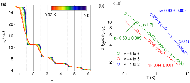
Figure S3: Scaling exponents in low mobility graphene device.(a) Plots of $R_{xy}$ versus filling factor at different temperatures. (b) Plots of d$R_{xy}/$d$\nu$ at the critical point $\nu=\nu_{C}$ versus temperature (log-log scale) for various plateau-to-plateau transitions. The values of $\kappa$ extracted from the plots are mentioned in the plot.

To compare the effect of long-range and short-range potential disorders [33] on the scaling exponents, we fabricated hBN-encapsulated graphene heterostructures without the back graphite electrode. The number density across these devices is tuned using a Si/SiO2 gate. Despite being hBN encapsulated, effects of Coulomb impurities present at the SiO2 surface containing dangling bonds are not screened. These lead to long-range potential fluctuations across the device [66, 37]. Fig. S3 shows the variation of d$R_{xy}/\mathrm{d}\nu$ at ${\nu=\nu_{c}}$ as a function of temperature for one such device for different plateau-to-plateau transitions. We observe a large spread in values of the scaling exponent $\kappa$, as opposed to the case of high-mobility devices discussed in the main manuscript, where the values of $\kappa$ were tightly clustered around the theoretically predicted value of $0.42$. Our analysis supports the recent observations where the presence of long-range interactions made the scaling exponent non-universal [36].

S5 Second derivative of $R_{xy}$ with temperature.

As discussed in the main manuscript, a single parameter scaling function can be written down for the resistance tensor for plateau-to-plateau transitions [67, 3, 68]:

$$R_{xy}(\nu,T)=R_{xy}(\nu_{c})f[T^{-\kappa}(\nu-\nu_{c})]$$ (S2)

This immediately leads to

$$\frac{\mathrm{d}R_{xy}}{\mathrm{d}\nu}\propto T^{-\kappa}$$ (S3)

and

$$\frac{\mathrm{d}^{2}R_{xy}}{\mathrm{d}\nu^{2}}\propto T^{-2\kappa}$$ (S4)

Fig. S4 (a) and (b) show plots of d${}^{2}R_{xy}/\mathrm{d}{\nu}^{2}$ as a function of temperature for two different plateau-to-plateau transitions. Fig. S4 (c) shows the variation of the d${}^{2}R_{xy}/\mathrm{d}{\nu}^{2}$ at $\nu=\nu_{c}$ with temperature in log-log scale. The slope yields $2\kappa\approx 0.83$, a value matching very closely with the prediction of Eqn. S4.

Figure S4: Second derivative of $R_{xy}$ with temperature. Plots of $\mathrm{d}^{2}R_{xy}/\mathrm{d}\nu^{2}$ vs $\nu$ at different temperatures for plateau-to-plateau transitions between between (a) $\nu=-1$ and $\nu=-2$ and (b) $\nu=-3$ and $\nu=-4$. (c) Log- log plot of $\mathrm{d}^{2}R_{xy}/\mathrm{d}\nu^{2}$ vs $T$ for three different PT (open circles). The dotted lines are the linear fits to the data.

S6 Fractional Quantum Hall states at $B=4.5$ T.

Fig. S5 plots the longitudinal resistance $R_{xx}$ as a function of filling factor $\nu$. We can see the emergence of FQH states at $\nu=n+1/3$ and $\nu=n+2/3$ at $B=4.5$ T.

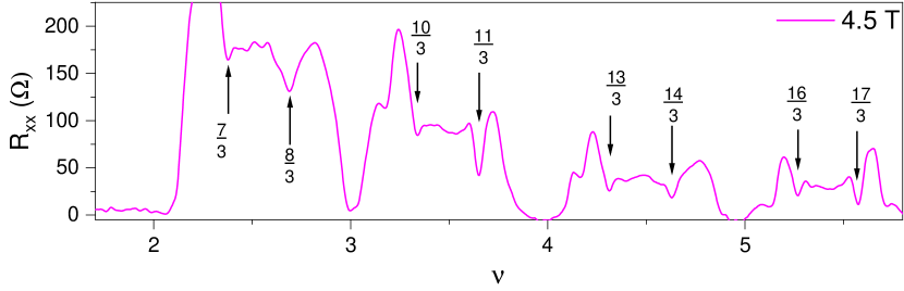
Figure S5: Fractional Quantum Hall states at $B=4.5$ T. Plot of $R_{xx}$ versus $\nu$ measured at $B=4.5$ T and $T=20$ mK. The major FQH that begin to form are marked by arrows.

S7 Details of scaling analysis.

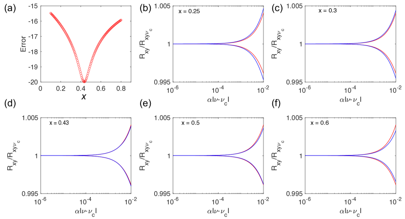
Figure S6: Scaling analysis for transition between $\nu=2+2/3$ and $\nu=2+3/5$. (a) Plot of the error in scaling versus $x$. (b-f) Scaling plot for different values of $x$ (the values of $x$ are marked inside the plot).

In this section, we describe the process followed to extract the value of $\kappa$. As discussed in the main manuscript, we use the following scaling equation [3]:

$$R_{xy}(\nu,T)=R_{xy}(\nu_{c})f[\alpha(\nu-\nu_{c})]$$ (S5)

with

$$\alpha\propto T^{-x}$$ (S6)

Fig. S6(b-f) shows $R_{xy}/R_{xy}(\nu_{c})$ at various temperatures as a function of $\alpha|\nu-\nu_{c}|$ for the $\nu=2+2/3$ to $2+3/5$ transition. The plots are for different values of $x$. The red line corresponds to $T=1.3$ K, and the blue line corresponds to $T=0.5$ K. For a perfect scaling, these two plots should collapse. However, it is challenging to visually determine the value of $x$ that achieves the best scaling. To address this, the variance between the two plots is calculated as an ’error’ metric for the scaling accuracy. We identify $\kappa$ with the value of $x$ that minimizes this error. In this specific instance, the optimum value is $\kappa=0.42$, as shown in Fig. S6(a).

S8 Values of $\kappa$ from previous studies

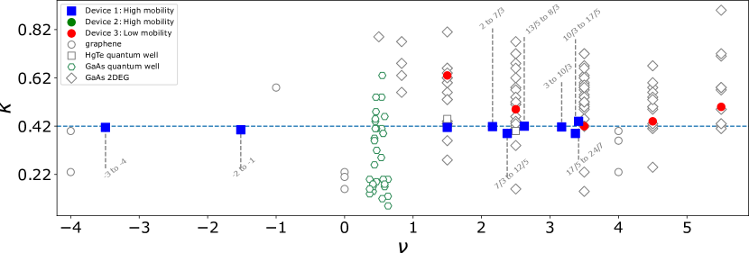
Figure S7: A compilation of the values of $\kappa$ from previous studies [69, 70, 2, 69, 71, 72, 73, 74, 75, 76, 77, 74, 75, 76, 78, 79, 80], represented by open symbols. The results of the current study are represented with filled squares and circles. Details of the data and the corresponding references are compiled in table LABEL:tab:my_label and table LABEL:tab:graphene.

Table S2: A compilation of the values of $\kappa$ obtained in 2D materials other than graphene by different groups.

PPT	$\kappa$	Material	Reference
1$\rightarrow$2/3	0.77$\pm$0.02	$\mathrm{Al_{x}Ga_{(1-x)}As-Al_{0:33}Ga_{0:67}As}$	[70]
1$\rightarrow$2/3	0.63$\pm$0.07	$\mathrm{Al_{x}Ga_{(1-x)}As-Al_{0:33}Ga_{0:67}As}$	[70]
1$\rightarrow$2/3	0.56$\pm$0.02	$\mathrm{Al_{x}Ga_{(1-x)}As-Al_{0:33}Ga_{0:67}As}$	[70]
1$\rightarrow$2/3	0.68$\pm$0.05	$\mathrm{Al_{x}Ga_{(1-x)}As-Al_{0:33}Ga_{0:67}As}$	[70]
1$\rightarrow$2	0.36$\pm$0.04	$\mathrm{Al_{x}Ga_{(1-x)}As-Al_{0:33}Ga_{0:67}As}$	[70]
1$\rightarrow$2	0.56$\pm$0.05	$\mathrm{Al_{x}Ga_{(1-x)}As-Al_{0:33}Ga_{0:67}As}$	[70]
1$\rightarrow$2	0.81$\pm$0.04	$\mathrm{Al_{x}Ga_{(1-x)}As-Al_{0:33}Ga_{0:67}As}$	[70]
1$\rightarrow$2	0.44$\pm$0.02	$\mathrm{Al_{x}Ga_{(1-x)}As-Al_{0:33}Ga_{0:67}As}$	[70]
1$\rightarrow$2	0.53$\pm$0.07	$\mathrm{Al_{x}Ga_{(1-x)}As-Al_{0:33}Ga_{0:67}As}$	[70]
1$\rightarrow$2	0.43$\pm$0.10	$\mathrm{Al_{x}Ga_{(1-x)}As-Al_{0:33}Ga_{0:67}As}$	[70]
1$\rightarrow$2	0.62$\pm$0.03	$\mathrm{Al_{x}Ga_{(1-x)}As-Al_{0:33}Ga_{0:67}As}$	[70]
1$\rightarrow$2	0.28$\pm$0.06	$\mathrm{Al_{x}Ga_{(1-x)}As-Al_{0:33}Ga_{0:67}As}$	[70]
1$\rightarrow$2	0.53$\pm$0.06	$\mathrm{Al_{x}Ga_{(1-x)}As-Al_{0:33}Ga_{0:67}As}$	[70]
1$\rightarrow$2	0.43$\pm$0.1	$\mathrm{Al_{x}Ga_{(1-x)}As-Al_{0:33}Ga_{0:67}As}$	[70]
2$\rightarrow$3	0.51$\pm$0.03	$\mathrm{Al_{x}Ga_{(1-x)}As-Al_{0:33}Ga_{0:67}As}$	[70]
3$\rightarrow$4	0.51$\pm$0.03	$\mathrm{Al_{x}Ga_{(1-x)}As-Al_{0:33}Ga_{0:67}As}$	[70]
3$\rightarrow$4	0.45$\pm$0.05	$\mathrm{Al_{x}Ga_{(1-x)}As-Al_{0:33}Ga_{0:67}As}$	[70]
3$\rightarrow$4	0.45$\pm$0.05	$\mathrm{Al_{x}Ga_{(1-x)}As-Al_{0:33}Ga_{0:67}As}$	[70]
3$\rightarrow$4	0.52$\pm$0.03	$\mathrm{Al_{x}Ga_{(1-x)}As-Al_{0:33}Ga_{0:67}As}$	[70]
3$\rightarrow$4	0.63$\pm$0.03	$\mathrm{Al_{x}Ga_{(1-x)}As-Al_{0:33}Ga_{0:67}As}$	[70]
1$\rightarrow$2	0.42$\pm$0.04	$\mathrm{In_{0.53}Ga_{0.47}As/InP}$	[69]
2$\rightarrow$3, 3$\rightarrow$4	0.42$\pm$0.04	$\mathrm{In_{0.53}Ga_{0.47}As/InP}$	[69]
2$\rightarrow$3	0.72$\pm$0.05	GaAs/AlGaAs	[81]
4$\rightarrow$5	0.25	GaAs/AlGaAs	[81]
3$\rightarrow$4	0.15	GaAs/AlGaAs	[81]
5$\rightarrow$6	0.9	GaAs/AlGaAs	[81]
2$\rightarrow$3,3$\rightarrow$4	0.62	GaAs/AlGaAs	[81]
1$\rightarrow$2,2$\rightarrow$3 3$\rightarrow$4	0.2 to 0.43	GaAs/AlGaAs	[81]
6$\rightarrow$5	0.71	GaAs/AlGaAs	[82]
7$\rightarrow$6	0.72	GaAs/AlGaAs	[82]
6$\rightarrow$5	0.74	GaAs/AlGaAs	[82]
7$\rightarrow$6	0.77	GaAs/AlGaAs	[82]
8$\rightarrow$10	0.75$\pm$0.05	GaAs/AlGaAs	[82]
1$\rightarrow$2	0.66$\pm$0.02	GaAs/AlGaAs	[83]
1$\rightarrow$2	0.6$\pm$0.02	GaAs/AlGaAs	[83]
1$\rightarrow$2	0.62$\pm$0.03	GaAs/AlGaAs	[83]
6$\rightarrow$5	0.58	$\mathrm{\mathrm{Al_{x}Ga_{1-x}As-Al_{0.33}Ga_{0.67}As(0\%Al)}}$	[33]
5$\rightarrow$4	0.58	${\mathrm{Al_{x}Ga_{1-x}As-Al_{0.33}Ga_{0.67}As(0\%Al)}}$	[33]
4$\rightarrow$3	0.57	$\mathrm{Al_{x}Ga_{1-x}As-Al_{0.33}Ga_{0.67}As(0\%Al)}$	[33]
6$\rightarrow$5	0.57	$\mathrm{Al_{x}Ga_{1-x}As-Al_{0.33}Ga_{0.67}As(0.21\%Al})$	[33]
5$\rightarrow$4	0.56	$\mathrm{Al_{x}Ga_{1-x}As-Al_{0.33}Ga_{0.67}As(0.21\%Al)}$	[33]
4$\rightarrow$3	0.58	$\mathrm{Al_{x}Ga_{1-x}As-Al_{0.33}Ga_{0.67}As(0.21\%Al)}$	[33]
6$\rightarrow$5	0.49	$\mathrm{Al_{x}Ga_{1-x}As-Al_{0.33}Ga_{0.67}As(0.33\%Al)}$	[33]
5$\rightarrow$4	0.5	$\mathrm{Al_{x}Ga_{1-x}As-Al_{0.33}Ga_{0.67}As(0.33\%Al)}$	[33]
4$\rightarrow$3	0.49	$\mathrm{Al_{x}Ga_{1-x}As-Al_{0.33}Ga_{0.67}As(0.33\%Al)}$	[33]
6$\rightarrow$5	0.43	$\mathrm{Al_{x}Ga_{1-x}As-Al_{0.33}Ga_{0.67}As(0.33\%Al)}$	[33]
5$\rightarrow$4	0.42	$\mathrm{Al_{x}Ga_{1-x}As-Al_{0.33}Ga_{0.67}As(0.33\%Al)}$	[33]
4$\rightarrow$3	0.42	$\mathrm{Al_{x}Ga_{1-x}As-Al_{0.33}Ga_{0.67}As(0.33\%Al)}$	[33]
3$\rightarrow$2	0.41	$\mathrm{Al_{x}Ga_{1-x}As-Al_{0.33}Ga_{0.67}As(0.33\%Al)}$	[33]
6$\rightarrow$5	0.42	$\mathrm{Al_{x}Ga_{1-x}As-Al_{0.33}Ga_{0.67}As(0.85\%Al)}$	[33]
5$\rightarrow$4	0.41	$\mathrm{Al_{x}Ga_{1-x}As-Al_{0.33}Ga_{0.67}As(0.85\%Al)}$	[33]
4$\rightarrow$3	0.42	$\mathrm{Al_{x}Ga_{1-x}As-Al_{0.33}Ga_{0.67}As(0.85\%Al)}$	[33]
3$\rightarrow$2	0.42	$\mathrm{Al_{x}Ga_{1-x}As-Al_{0.33}Ga_{0.67}As(0.85\%Al)}$	[33]
6$\rightarrow$5	0.42	$\mathrm{Al_{x}Ga_{1-x}As-Al_{0.33}Ga_{0.67}As(0.85\%Al)}$	[33]
5$\rightarrow$4	0.42	$\mathrm{Al_{x}Ga_{1-x}As-Al_{0.33}Ga_{0.67}As(0.85\%Al)}$	[33]
4$\rightarrow$3	0.42	${Al_{x}Ga_{1-x}As-Al_{0.33}Ga_{0.67}As(0.85\%Al)}$	[33]
3$\rightarrow$2	0.41	$\mathrm{Al_{x}Ga_{1-x}As-Al_{0.33}Ga_{0.67}As(0.85\%Al)}$	[33]
6$\rightarrow$5	0.41	$\mathrm{Al_{x}Ga_{1-x}As-Al_{0.33}Ga_{0.67}As(0.85\%Al)}$	[33]
5$\rightarrow$4	0.42	$\mathrm{Al_{x}Ga_{1-x}As-Al_{0.33}Ga_{0.67}As(0.85\%Al)}$	[33]
4$\rightarrow$3	0.42	$\mathrm{Al_{x}Ga_{1-x}As-Al_{0.33}Ga_{0.67}As(0.85\%Al)}$	[33]
3$\rightarrow$2	0.42	$\mathrm{Al_{x}Ga_{1-x}As-Al_{0.33}Ga_{0.67}As(0.85\%Al)}$	[33]
6$\rightarrow$5	0.43	$\mathrm{Al_{x}Ga_{1-x}As-Al_{0.33}Ga_{0.67}As(1.4\%Al)}$	[33]
5$\rightarrow$4	0.43	$\mathrm{Al_{x}Ga_{1-x}As-Al_{0.33}Ga_{0.67}As(1.4\%Al)}$	[33]
4$\rightarrow$3	0.42	$\mathrm{Al_{x}Ga_{1-x}As-Al_{0.33}Ga_{0.67}As(1.4\%Al)}$	[33]
3$\rightarrow$2	0.42	$\mathrm{Al_{x}Ga_{1-x}As-Al_{0.33}Ga_{0.67}As(1.4\%Al)}$	[33]
6$\rightarrow$5	0.49	$\mathrm{Al_{x}Ga_{1-x}As-Al_{0.33}Ga_{0.67}As(1.9\%Al)}$	[33]
5$\rightarrow$4	0.49	$\mathrm{Al_{x}Ga_{1-x}As-Al_{0.33}Ga_{0.67}As(1.9\%Al)}$	[33]
4$\rightarrow$3	0.5	$\mathrm{Al_{x}Ga_{1-x}As-Al_{0.33}Ga_{0.67}As(1.9\%Al)}$	[33]
3$\rightarrow$2	0.51	$\mathrm{Al_{x}Ga_{1-x}As-Al_{0.33}Ga_{0.67}As(1.9\%Al)}$	[33]
6$\rightarrow$5	0.58	$\mathrm{Al_{x}Ga_{1-x}As-Al_{0.33}Ga_{0.67}As(2.6\%Al)}$	[33]
5$\rightarrow$4	0.6	$\mathrm{Al_{x}Ga_{1-x}As-Al_{0.33}Ga_{0.67}As(2.6\%Al)}$	[33]
4$\rightarrow$3	0.59	$\mathrm{Al_{x}Ga_{1-x}As-Al_{0.33}Ga_{0.67}As(2.6\%Al)}$	[33]
3$\rightarrow$2	0.58	$\mathrm{Al_{x}Ga_{1-x}As-Al_{0.33}Ga_{0.67}As(2.6\%Al)}$	[33]
4$\rightarrow$3	0.58	$\mathrm{Al_{x}Ga_{1-x}As-Al_{0.33}Ga_{0.67}As(4.1\%Al)}$	[33]
3$\rightarrow$2	0.57	$\mathrm{Al_{x}Ga_{1-x}As-Al_{0.33}Ga_{0.67}As~{}(4.1\%Al)}$	[33]
4$\rightarrow$3	0.42$\pm$0.01	GaAs/AlGaAs	[30]
4$\rightarrow$3	0.67$\pm$0.02	GaAs/AlGaAs	[30]
4$\rightarrow$3	0.55$\pm$0.04	GaAs/AlGaAs	[30]
4$\rightarrow$3	0.54$\pm$0.02	GaAs/AlGaAs	[30]
4$\rightarrow$3	0.23$\pm$0.02	GaAs/AlGaAs	[30]
4$\rightarrow$3	0.66$\pm$0.03	GaAs/AlGaAs	[30]
4$\rightarrow$3	0.60$\pm$0.02	GaAs/AlGaAs	[30]
4$\rightarrow$3	0.54$\pm$0.02	GaAs/AlGaAs	[30]
3$\rightarrow$2	0.41$\pm$0.01	GaAs/AlGaAs	[30]
3$\rightarrow$2	0.44$\pm$0.02	GaAs/AlGaAs	[30]
3$\rightarrow$2	0.46$\pm$0.02	GaAs/AlGaAs	[30]
3$\rightarrow$2	0.34$\pm$0.01	GaAs/AlGaAs	[30]
3$\rightarrow$2	0.44$\pm$0.02	GaAs/AlGaAs	[30]
3$\rightarrow$2	0.42$\pm$0.03	GaAs/AlGaAs	[30]
3$\rightarrow$2	0.43$\pm$0.03	GaAs/AlGaAs	[30]
3$\rightarrow$2	0.16$\pm$0.02	GaAs/AlGaAs	[30]
2/3$\rightarrow$3/5	0.09	GaAs quantum wells (50nm)	[36]
3/5$\rightarrow$4/7	0.46	GaAs quantum wells (50nm)	[36]
4/7$\rightarrow$5/9	0.39	GaAs quantum wells (50nm)	[36]
6/11$\rightarrow$5/9	0.41	GaAs quantum wells (50nm)	[36]
7/13$\rightarrow$8/15	0.29	GaAs quantum wells (50nm)	[36]
7/15$\rightarrow$6/13	0.19	GaAs quantum wells (50nm)	[36]
6/13$\rightarrow$5/11	0.48	GaAs quantum wells (50nm)	[36]
5/11$\rightarrow$4/9	0.44	GaAs quantum wells (50nm)	[36]
4/9$\rightarrow$3/7	0.37	GaAs quantum wells (50nm)	[36]
3/7$\rightarrow$2/5	0.15	GaAs quantum wells (50nm)	[36]
2/5$\rightarrow$1/3	0.14	GaAs quantum wells (50nm)	[36]
2/3$\rightarrow$3/5	0.20	GaAs quantum wells (30nm)	[36]
3/5$\rightarrow$4/7	0.17	GaAs quantum wells (30nm)	[36]
4/7$\rightarrow$5/9	0.20	GaAs quantum wells (30nm)	[36]
5/9$\rightarrow$6/11	0.63	GaAs quantum wells (30nm)	[36]
6/11$\rightarrow$7/13	0.54	GaAs quantum wells (30nm)	[36]
7/15$\rightarrow$8/17	0.32	GaAs quantum wells (30nm)	[36]
6/13$\rightarrow$7/15	0.41	GaAs quantum wells (30nm)	[36]
6/13$\rightarrow$5/11	0.54	GaAs quantum wells (30nm)	[36]
5/11$\rightarrow$4/9	0.41	GaAs quantum wells (30nm)	[36]
4/9$\rightarrow$3/7	0.26	GaAs quantum wells (30nm)	[36]
3/7$\rightarrow$2/5	0.17	GaAs quantum wells (30nm)	[36]
2/5$\rightarrow$1/3	0.20	GaAs quantum wells (30nm)	[36]
2/3$\rightarrow$3/5	0.13	GaAs quantum wells (40nm)	[36]
3/5$\rightarrow$4/7	0.18	GaAs quantum wells (40nm)	[36]
4/7$\rightarrow$5/9	0.39	GaAs quantum wells (40nm)	[36]
5/9$\rightarrow$6/11	0.12	GaAs quantum wells (40nm)	[36]
5/11$\rightarrow$4/9	0.45	GaAs quantum wells (40nm)	[36]
4/9$\rightarrow$3/7	0.36	GaAs quantum wells (40nm)	[36]
3/7$\rightarrow$2/5	0.18	GaAs quantum wells (40nm)	[36]
2/5$\rightarrow$1/3	0.16	GaAs quantum wells (40nm)	[36]
2$\rightarrow$1	0.42	GaAs/AlGaAs	[84]
3$\rightarrow$2	0.72$\pm$0.2	GaAs/AlGaAs	[84]
4$\rightarrow$3	0.72$\pm$0.2	GaAs/AlGaAs	[84]
3$\rightarrow$2	0.68$\pm$0.04	GaAs/AlGaAs	[85]
4$\rightarrow$3	0.72$\pm$0.05	GaAs/AlGaAs	[85]
5$\rightarrow$4	0.67$\pm$0.06	GaAs/AlGaAs	[85]
4$\rightarrow$3	0.5 $\pm$0.03	GaAs/AlGaAs	[86]
5$\rightarrow$4	0.5$\pm$0.03	GaAs/AlGaAs	[86]
4$\rightarrow$3	0.62 $\pm$0.04	GaAs/AlGaAs	[87]
4$\rightarrow$3	0.59$\pm$0.04	GaAs/AlGaAs	[87]
2$\rightarrow$1	0.66$\pm$0.02	GaAs/AlGaAs	[83]
2$\rightarrow$1	0.60$\pm$0.0	GaAs/AlGaAs	[83]
2$\rightarrow$1	0.62$\pm$0.02	GaAs/AlGaAs	[83]
2$\rightarrow$1	0.64 $\pm$0.09	GaAs/AlGaAs	[88]
3$\rightarrow$2	0.66 - 0.77	GaAs/AlGaAs	[89]
6$\rightarrow$5	0.72(0.74)	GaAs/AlGaAs	[82]
7$\rightarrow$6	0.72(0.80)	GaAs/AlGaAs	[82]
8$\rightarrow$7	0.75 $\pm$0.05	GaAs/AlGaAs	[82]
1$\rightarrow$0	0.79	GaAs/AlGaAs	[90]
3$\rightarrow$2	0.54	GaAs/AlGaAs	[90]
4$\rightarrow$3	0.42	GaAs/AlGaAs	[91]
4$\rightarrow$3	0.58	GaAs/AlGaAs	[91]
3$\rightarrow$2	0.52$\pm$0.01	GaAs/AlGaAs	[92]
4$\rightarrow$3	0.52$\pm$0.02	GaAs/AlGaAs	[92]
5$\rightarrow$4	0.53$\pm$0.02	GaAs/AlGaAs	[92]
1$\rightarrow$2	0.45$\pm$0.04	HgTe Quantum wells (5.9 nm)	[93]
2$\rightarrow$3	0.40$\pm$0.02	HgTe Quantum wells (5.9 nm)	[93]

Table S3: Values of $\kappa$ obtained in graphene from previous studies. The results of our present study are also included.

PPT	$\kappa$	Material	Reference
2 $\rightarrow$ 6	0.23$\pm$0.02	Graphene on SiO_2	[94]
-2 $\rightarrow$ -6	0.23$\pm$0.02	Graphene on SiO_2	[94]
-10 $\rightarrow$ -6	0.23$\pm$0.02	Graphene on SiO_2	[94]
10 $\rightarrow$ 6	0.23$\pm$0.02	Graphene on SiO_2	[94]
-2 $\rightarrow$ 2	0.23$\pm$0.02	Graphene on SiO_2	[94]
6 $\rightarrow$ 10	0.40$\pm$0.04	Graphene on SiO_2	[71]
2 $\rightarrow$ 6	0.40$\pm$0.04	Graphene on SiO_2	[71]
-2 $\rightarrow$ -6	0.40$\pm$0.03	Graphene on SiO_2	[71]
-6 $\rightarrow$ -10	0.40$\pm$0.03	Graphene on SiO_2	[71]
6 $\rightarrow$ 10	0.41$\pm$0.03	Graphene on SiO_2	[71]
-2 $\rightarrow$ 2	0.16$\pm$0.05	Graphene on SiO_2 Corbino geometry	[74]
-2 $\rightarrow$ 0	0.58 $\pm$ 0.03	Graphene on SiO_2 (hall bar)	[95]
-2 $\rightarrow$ 2	0.21$\pm$0.01	Graphene (pnp junction)	[75]
2 $\rightarrow$ 6	0.36$\pm$0.01	Graphene (pnp junction)	[75]
6 $\rightarrow$ 10	0.35$\pm$0.01	Graphene (pnp junction)	[75]
16 $\rightarrow$ 12	0.27$\pm$0.01	Encapsulated BLG	[78]
12 $\rightarrow$ 8	0.32$\pm$0.01	Encapsulated BLG	[78]
16 $\rightarrow$ 12	0.30$\pm$0.01	Encapsulated BLG	[78]
12 $\rightarrow$ 8	0.32$\pm$0.01	Encapsulated BLG	[78]
-8 $\rightarrow$ -4	0.30$\pm$0.02	Encapsulated BLG	[78]
-8 $\rightarrow$ -4	0.29$\pm$0.02	Encapsulated BLG	[78]
-16 $\rightarrow$-12	0.32$\pm$0.02	Encapsulated BLG	[78]
-4 $\rightarrow$-3	0.41$\pm$0.006	Current study (high mobility)	current study
-2 $\rightarrow$-1	0.40$\pm$0.005	Current study (high mobility)	current study
2$\rightarrow$7/3	0.42$\pm$0.004	Current study (high mobility)	current study
7/3$\rightarrow$12/5	0.38$\pm$0.02	Current study (high mobility)	current study
10/3$\rightarrow$17/5	0.39$\pm$0.03	Current study (high mobility)	current study
13/5$\rightarrow$8/3	0.42$\pm$0.01	Current study (high mobility)	current study
3$\rightarrow$10/3	0.42$\pm$0.009	Current study (high mobility)	current study
17/5$\rightarrow$24/7	0.44$\pm$0.02	Current study (high mobility)	current study
1$\rightarrow$2	0.41$\pm$0.007	Current study (high mobility)	current study
1$\rightarrow$2	0.63$\pm$0.006	Current study (low mobility)	current study
2$\rightarrow$3	0.49$\pm$0.01	Current study (low mobility)	current study
3$\rightarrow$4	0.42$\pm$0.009	Current study (low mobility)	current study
4$\rightarrow$5	0.44$\pm$0.01	Current study (low mobility)	current study
5$\rightarrow$6	0.50$\pm$0.009	Current study (low mobility)	current study

References

- Klitzing et al. [1980] K. v. Klitzing, G. Dorda, and M. Pepper, Phys. Rev. Lett. 45, 494 (1980).
- Li et al. [2009] W. Li, C. L. Vicente, J. S. Xia, W. Pan, D. C. Tsui, L. N. Pfeiffer, and K. W. West, Phys. Rev. Lett. 102, 216801 (2009).
- Huckestein [1995] B. Huckestein, Rev. Mod. Phys. 67, 357 (1995).
- Tsui et al. [1982a] D. C. Tsui, H. L. Stormer, and A. C. Gossard, Phys. Rev. Lett. 48, 1559 (1982a).
- Serbyn and Abanin [2013] M. Serbyn and D. A. Abanin, Phys. Rev. B 87, 115422 (2013).
- Campos et al. [2016] L. C. Campos, T. Taychatanapat, M. Serbyn, K. Surakitbovorn, K. Watanabe, T. Taniguchi, D. A. Abanin, and P. Jarillo-Herrero, Phys. Rev. Lett. 117, 066601 (2016).
- Evers and Mirlin [2008] F. Evers and A. D. Mirlin, Rev. Mod. Phys. 80, 1355 (2008).
- Jain et al. [1990] J. K. Jain, S. A. Kivelson, and N. Trivedi, Phys. Rev. Lett. 64, 1297 (1990).
- Pu et al. [2022] S. Pu, G. J. Sreejith, and J. K. Jain, Phys. Rev. Lett. 128, 116801 (2022).
- Kumar et al. [2022] P. Kumar, P. A. Nosov, and S. Raghu, Phys. Rev. Res. 4, 033146 (2022).
- Han et al. [2023] T. Han, Z. Lu, G. Scuri, J. Sung, J. Wang, T. Han, K. Watanabe, T. Taniguchi, H. Park, and L. Ju, Nature Nanotechnology 10.1038/s41565-023-01520-1 (2023).
- Li et al. [2017] J. I. A. Li, C. Tan, S. Chen, Y. Zeng, T. Taniguchi, K. Watanabe, J. Hone, and C. R. Dean, Science 358, 648 (2017), https://www.science.org/doi/pdf/10.1126/science.aao2521 .
- Huo and Bhatt [1992] Y. Huo and R. N. Bhatt, Phys. Rev. Lett. 68, 1375 (1992).
- Laughlin [1981] R. B. Laughlin, Phys. Rev. B 23, 5632 (1981).
- Aoki and Ando [1985] H. Aoki and T. Ando, Phys. Rev. Lett. 54, 831 (1985).
- Chalker and Daniell [1988a] J. T. Chalker and G. J. Daniell, Phys. Rev. Lett. 61, 593 (1988a).
- Chalker and Coddington [1988] J. T. Chalker and P. D. Coddington, Journal of Physics C: Solid State Physics 21, 2665 (1988).
- Huckestein and Backhaus [1999] B. Huckestein and M. Backhaus, Phys. Rev. Lett. 82, 5100 (1999).
- Janseen [1994] M. Janseen, International Journal of Modern Physics B 08, 943 (1994).
- Pruisken [1988a] A. M. M. Pruisken, Phys. Rev. Lett. 61, 1297 (1988a).
- Chalker and Daniell [1988b] J. T. Chalker and G. J. Daniell, Phys. Rev. Lett. 61, 10.1103/PhysRevLett.61.593 (1988b).
- Nakayama and Yakubo [2013] T. Nakayama and K. Yakubo, Fractal Concepts in Condensed Matter Physics, Springer Series in Solid-State Sciences (Springer Berlin Heidelberg, 2013).
- Amin et al. [2022] K. R. Amin, R. Nagarajan, R. Pandit, and A. Bid, Phys. Rev. Lett. 129, 186802 (2022).
- Barbosa et al. [2022] A. L. R. Barbosa, T. H. V. de Lima, I. R. R. González, N. L. Pessoa, A. M. S. Macêdo, and G. L. Vasconcelos, Phys. Rev. Lett. 128, 236803 (2022).
- Tsui et al. [1982b] D. C. Tsui, H. L. Stormer, and A. C. Gossard, Phys. Rev. Lett. 48, 1559 (1982b).
- Jain [1989a] J. K. Jain, Phys. Rev. Lett. 63, 199 (1989a).
- Kivelson et al. [1992] S. Kivelson, D.-H. Lee, and S.-C. Zhang, Phys. Rev. B 46, 2223 (1992).
- Hui et al. [2019] A. Hui, E.-A. Kim, and M. Mulligan, Phys. Rev. B 99, 125135 (2019).
- Sondhi et al. [1997] S. L. Sondhi, S. M. Girvin, J. P. Carini, and D. Shahar, Rev. Mod. Phys. 69, 315 (1997).
- Dodoo-Amoo et al. [2014] N. A. Dodoo-Amoo, K. Saeed, D. Mistry, S. P. Khanna, L. Li, E. H. Linfield, A. G. Davies, and J. E. Cunningham, Journal of Physics: Condensed Matter 26, 475801 (2014).
- Huckestein and Kramer [1990] B. Huckestein and B. Kramer, Phys. Rev. Lett. 64, 1437 (1990).
- Wei et al. [1992a] H. P. Wei, S. Y. Lin, D. C. Tsui, and A. M. M. Pruisken, Phys. Rev. B 45, 3926 (1992a).
- Li et al. [2005] W. Li, G. A. Csáthy, D. C. Tsui, L. N. Pfeiffer, and K. W. West, Phys. Rev. Lett. 94, 206807 (2005).
- Engel et al. [1990] L. Engel, H. Wei, D. Tsui, and M. Shayegan, Surface science 229, 13 (1990).
- Machida et al. [2001] T. Machida, S. Ishizuka, S. Komiyama, K. Muraki, and Y. Hirayama, Physica B: Condensed Matter 298, 182 (2001), international Conference on High Magnetic Fields in Semiconductors.
- Madathil et al. [2023] P. T. Madathil, K. A. Villegas Rosales, C. T. Tai, Y. J. Chung, L. N. Pfeiffer, K. W. West, K. W. Baldwin, and M. Shayegan, Phys. Rev. Lett. 130, 226503 (2023).
- Sarkar et al. [2015] S. Sarkar, K. R. Amin, R. Modak, A. Singh, S. Mukerjee, and A. Bid, Scientific Reports 5, 16772 (2015).
- Stepanov et al. [2016] P. Stepanov, Y. Barlas, T. Espiritu, S. Che, K. Watanabe, T. Taniguchi, D. Smirnov, and C. N. Lau, Phys. Rev. Lett. 117, 076807 (2016).
- Pizzocchero et al. [2016] F. Pizzocchero, L. Gammelgaard, B. S. Jessen, J. M. Caridad, L. Wang, J. Hone, P. Bøggild, and T. J. Booth, Nature communications 7, 11894 (2016).
- Koshino and McCann [2011] M. Koshino and E. McCann, Physical Review B 83, 165443 (2011).
- Papić et al. [2011] Z. Papić, D. A. Abanin, Y. Barlas, and R. N. Bhatt, Phys. Rev. B 84, 241306 (2011).
- Zhu et al. [2020] Z. Zhu, D. N. Sheng, and I. Sodemann, Phys. Rev. Lett. 124, 097604 (2020).
- Sodemann and MacDonald [2013] I. Sodemann and A. H. MacDonald, Phys. Rev. B 87, 245425 (2013).
- Halperin and Hohenberg [1969] B. I. Halperin and P. C. Hohenberg, Phys. Rev. 177, 952 (1969).
- Goldman et al. [1990a] V. J. Goldman, J. K. Jain, and M. Shayegan, Phys. Rev. Lett. 65, 907 (1990a).
- Zibrov et al. [2018] A. A. Zibrov, P. Rao, C. Kometter, E. M. Spanton, J. Li, C. R. Dean, T. Taniguchi, K. Watanabe, M. Serbyn, and A. F. Young, Physical Review Letters 121, 167601 (2018).
- Rao and Serbyn [2020] P. Rao and M. Serbyn, Physical Review B 101, 245411 (2020).
- Winterer et al. [2022] F. Winterer, A. M. Seiler, A. Ghazaryan, F. R. Geisenhof, K. Watanabe, T. Taniguchi, M. Serbyn, and R. T. Weitz, Nano Letters 22, 3317 (2022).
- Wang et al. [2016a] Y.-P. Wang, X.-G. Li, J. N. Fry, and H.-P. Cheng, Physical Review B 94, 165428 (2016a).
- Jain [1989b] J. K. Jain, Phys. Rev. B 40, 8079 (1989b).
- Wu et al. [2017] Y.-H. Wu, T. Shi, and J. K. Jain, Nano Letters 17, 4643 (2017).
- Kim et al. [2019] Y. Kim, A. C. Balram, T. Taniguchi, K. Watanabe, J. K. Jain, and J. H. Smet, Nature Physics 15, 154 (2019).
- Cong et al. [2011] C. Cong, T. Yu, K. Sato, J. Shang, R. Saito, G. F. Dresselhaus, and M. S. Dresselhaus, ACS Nano 5, 8760 (2011), https://doi.org/10.1021/nn203472f .
- Nguyen et al. [2014] T. A. Nguyen, J.-U. Lee, D. Yoon, and H. Cheong, Scientific reports 4, 4630 (2014).
- Wang et al. [2013] L. Wang, I. Meric, P. Huang, Q. Gao, Y. Gao, H. Tran, T. Taniguchi, K. Watanabe, L. Campos, D. Muller, et al., Science 342, 614 (2013).
- Tiwari et al. [2021] P. Tiwari, S. P. Srivastav, and A. Bid, Phys. Rev. Lett. 126, 096801 (2021).
- Lui et al. [2011] C. H. Lui, Z. Li, K. F. Mak, E. Cappelluti, and T. F. Heinz, Nature Physics 7, 944 (2011).
- Datta et al. [2018] B. Datta, H. Agarwal, A. Samanta, A. Ratnakar, K. Watanabe, T. Taniguchi, R. Sensarma, and M. M. Deshmukh, Physical Review Letters 121, 056801 (2018).
- Chen et al. [2019] G. Chen, L. Jiang, S. Wu, B. Lyu, H. Li, B. L. Chittari, K. Watanabe, T. Taniguchi, Z. Shi, J. Jung, et al., Nature Physics 15, 237 (2019).
- Zhou et al. [2021] H. Zhou, T. Xie, T. Taniguchi, K. Watanabe, and A. F. Young, Nature 598, 434 (2021).
- Zou et al. [2013] K. Zou, F. Zhang, C. Clapp, A. MacDonald, and J. Zhu, Nano letters 13, 369 (2013).
- Jhang et al. [2011] S. H. Jhang, M. F. Craciun, S. Schmidmeier, S. Tokumitsu, S. Russo, M. Yamamoto, Y. Skourski, J. Wosnitza, S. Tarucha, J. Eroms, and C. Strunk, Physical Review B 84, 161408 (2011).
- Polyakov and Shklovskii [1993] D. G. Polyakov and B. I. Shklovskii, Phys. Rev. Lett. 70, 3796 (1993).
- Taychatanapat et al. [2011] T. Taychatanapat, K. Watanabe, T. Taniguchi, and P. Jarillo-Herrero, Nature Physics 7, 621 (2011).
- Goldman et al. [1990b] V. Goldman, J. K. Jain, and M. Shayegan, Phys. Rev. Lett. 65, 907 (1990b).
- Martin et al. [2008] J. Martin, N. Akerman, G. Ulbricht, T. Lohmann, J. H. Smet, K. von Klitzing, and A. Yacoby, Nature Physics 4, 144 (2008).
- Pruisken [1988b] A. Pruisken, Physical review letters 61, 1297 (1988b).
- Wei et al. [1990] H. Wei, S. Hwang, D. Tsui, and A. Pruisken, Surface Science 229, 34 (1990).
- Wei et al. [1988] H. P. Wei, D. C. Tsui, M. A. Paalanen, and A. M. M. Pruisken, Phys. Rev. Lett. 61, 1294 (1988).
- Koch et al. [1991a] S. Koch, R. J. Haug, K. v. Klitzing, and K. Ploog, Phys. Rev. B 43, 6828 (1991a).
- Giesbers et al. [2009] A. J. M. Giesbers, U. Zeitler, L. A. Ponomarenko, R. Yang, K. S. Novoselov, A. K. Geim, and J. C. Maan, Phys. Rev. B 80, 241411 (2009).
- Shen et al. [2012] T. Shen, A. T. Neal, M. L. Bolen, J. J. Gu, L. W. Engel, M. A. Capano, and P. D. Ye, Journal of Applied Physics 111, 013716 (2012).
- Pallecchi et al. [2013] E. Pallecchi, M. Ridene, D. Kazazis, F. Lafont, F. Schopfer, W. Poirier, M. O. Goerbig, D. Mailly, and A. Ouerghi, Scientific Reports 3, 1791 (2013).
- Peters et al. [2014] E. C. Peters, A. J. M. Giesbers, M. Burghard, and K. Kern, Appl. Phys. Lett. 104, 203109 (2014).
- Liu et al. [2016] C.-H. Liu, P.-H. Wang, T.-P. Woo, F.-Y. Shih, S.-C. Liou, P.-H. Ho, C.-W. Chen, C.-T. Liang, and W.-H. Wang, Phys. Rev. B 93, 041421 (2016).
- Amado et al. [2012] M. Amado, E. Diez, F. Rossella, V. Bellani, D. Lopez-Romero, and D. K. Maude, Journal of Physics: Condensed Matter 24, 305302 (2012).
- Jabakhanji et al. [2014] B. Jabakhanji, A. Michon, C. Consejo, W. Desrat, M. Portail, A. Tiberj, M. Paillet, A. Zahab, F. Cheynis, F. Lafont, F. Schopfer, W. Poirier, F. Bertran, P. Le Févre, A. Taleb-Ibrahimi, D. Kazazis, W. Escoffier, B. C. Camargo, Y. Kopelevich, J. Camassel, and B. Jouault, Phys. Rev. B 89, 085422 (2014).
- Cobaleda et al. [2014] C. Cobaleda, S. Pezzini, A. Rodriguez, E. Diez, and V. Bellani, Phys. Rev. B 90, 161408 (2014).
- Dresselhaus et al. [2021] E. J. Dresselhaus, B. Sbierski, and I. A. Gruzberg, Annals of Physics 435, 168676 (2021), special Issue on Localisation 2020.
- Zirnbauer [2019] M. R. Zirnbauer, Nuclear Physics B 941, 458 (2019).
- Koch et al. [1992] S. Koch, R. J. Haug, K. v. Klitzing, and K. Ploog, Phys. Rev. B 46, 1596 (1992).
- Zhao et al. [2008] Y. J. Zhao, T. Tu, X. J. Hao, G. C. Guo, H. W. Jiang, and G. P. Guo, Phys. Rev. B 78, 233301 (2008).
- Hohls et al. [2002] F. Hohls, U. Zeitler, and R. J. Haug, Phys. Rev. Lett. 88, 036802 (2002).
- Wei et al. [1992b] H. P. Wei, S. Y. Lin, D. C. Tsui, and A. M. M. Pruisken, Phys. Rev. B 45, 3926 (1992b).
- Koch et al. [1991b] S. Koch, R. J. Haug, K. v. Klitzing, and K. Ploog, Phys. Rev. Lett. 67, 883 (1991b).
- Yoo et al. [1994] K.-H. Yoo, H. Kwon, and J. Park, Solid State Communications 92, 821 (1994).
- Koch et al. [1995] S. Koch, R. J. Haug, K. von Klitzing, and K. Ploog, Semiconductor Science and Technology 10, 209 (1995).
- Huang et al. [2004] C. Huang, Y. Chang, H. Cheng, C.-T. Liang, and G. Hwang, Physica E: Low-dimensional Systems and Nanostructures 22, 232 (2004), 15th International Conference on Electronic Propreties of Two-Dimensional Systems (EP2DS-15).
- Tu et al. [2007] T. Tu, Y.-J. Zhao, G.-P. Guo, X.-J. Hao, and G.-C. Guo, Physics Letters A 368, 108 (2007).
- Nakajima et al. [2007] T. Nakajima, T. Ueda, and S. Komiyama, Journal of the Physical Society of Japan 76, 094703 (2007), https://doi.org/10.1143/JPSJ.76.094703 .
- Li et al. [2010] W. Li, J. S. Xia, C. Vicente, N. S. Sullivan, W. Pan, D. C. Tsui, L. N. Pfeiffer, and K. W. West, Phys. Rev. B 81, 033305 (2010).
- Wang et al. [2016b] X. Wang, H. Liu, J. Zhu, P. Shan, P. Wang, H. Fu, L. Du, L. N. Pfeiffer, K. W. West, X. C. Xie, R.-R. Du, and X. Lin, Phys. Rev. B 93, 075307 (2016b).
- Khouri et al. [2016] T. Khouri, M. Bendias, P. Leubner, C. Brüne, H. Buhmann, L. W. Molenkamp, U. Zeitler, N. E. Hussey, and S. Wiedmann, Phys. Rev. B 93, 125308 (2016).
- Bennaceur et al. [2012] K. Bennaceur, P. Jacques, F. Portier, P. Roche, and D. C. Glattli, Phys. Rev. B 86, 085433 (2012).
- Amado et al. [2010] M. Amado, E. Diez, D. López-Romero, F. Rossella, J. Caridad, F. Dionigi, V. Bellani, and D. Maude, New Journal of Physics 12, 053004 (2010).