Consistent combination of truncated-unity functional renormalization group and mean-field theory

Abstract

We propose a novel scheme for combining efficiently the truncated-unity functional renormalization group (TUFRG) and the mean-field theory. It follows a method of Wang, Eberlein and Metzner that uses only the two-particle irreducible part of the vertex as an input for the mean-field treatment. In the TUFRG, the neglect of fluctuation effects from other channels in the symmetry-broken regime is represented by applying the random phase approximation (RPA) in each individual channel, below the divergence scale. Then the Bethe-Salpeter equation for the four-point vertex is translated into the RPA matrix equations for the bosonic propagators that relates the singular and irreducible singular modes of the propagators. The universal symmetries for the irreducible singular modes are obtained from the antisymmetry of Grassmann variables. The mean-field equation based on these modes is derived by the saddle-point approximation in the framework of the path-integral formalism. By using our scheme, the power of the TUFRG, as an unbiased tool for identifying the many-body instabilities, could be elevated to a quantitative level, and its application would be extended to a quantitative analysis of the coexisting orders. As an illustration we employ this scheme to study the coexistence phase of the chiral superconductivity and the chiral spin-density wave, predicted near van Hove filling of the honeycomb lattice.

I Introduction

Intermediately correlated electron systems exhibit a plethora of fascinating properties and their theoretical analysis continue to be one of the important tasks in condensed matter physics. The systems can be described within both itinerant and strong coupling approaches. Among the itinerant approaches, the functional renormalization group (FRG) has proven to be an effective and reliable tool to study Fermi-surface instabilities in an unbiased way Metzner et al. (2012); Platt et al. (2013); Dupuis et al. (2021). It treats the pairing, spin and charge channels on equal footing, and thus enables to investigate the fluctuation-driven instabilities and competing or coexisting orders Eberlein (2014). The FRG method has been successfully applied to capture the $d$-wave pairing instability in the two-dimensional (2D) repulsive Hubbard model Zanchi and Schulz (2000); Halboth and Metzner (2000); Honerkamp et al. (2001); Eberlein and Metzner (2014) and the extended $s$-wave superconductivity (SC) in Fe-based superconductors Wang et al. (2009); Thomale et al. (2009); Platt et al. (2009).

In these FRG studies the evolution of the four-point vertex was approximated by a one-loop truncation, where the six-point and the higher-order vertices are completely neglected. Furthermore, in many FRG calculations one applies additional approximations of discarding the frequency dependence of and the self-energy feedback to the four-point vertex. They are justified in weak coupling regime by the fact that the frequency dependence appears, in its power counting, to be irrelevant Dupuis et al. (2021); Shankar (1994), and the higher-order vertices and the self-energy correction can only make contributions of third order in the bare interaction Metzner et al. (2012); Platt et al. (2013). We will also use these approximations in the present work.

In the FRG method, Fermi-surface instabilities are signaled by divergences of the four-point vertex at a divergence energy scale $\Omega_{D}$. The FRG flow of the four-point vertex should be stopped at this scale, because when the vertex becomes very large, the one-loop approximation is not valid any more. To complete the calculation and perform a quantitative analysis of resulting ordered phases, one has to continue the flow below the divergence scale $\Omega_{D}$, allowing the emergence of the symmetry-broken phase. This task can be accomplished by using either of two approaches, within a purely fermionic or a partially bosonized formalism.

In the first approach Salmhofer et al. (2004), one inserts an infinitesimal symmetry-breaking component into the initial action and tracks the FRG flow of purely fermionic vertex functions. It has been applied to obtain the exact solutions of the mean-field (MF) models for superconductivity Salmhofer et al. (2004); Honerkamp and Salmhofer (2005), and to describe a formation of $s$-wave superfluid phase in the 2D attracting Hubbard model Gersch et al. (2008); Eberlein and Metzner (2013). That scheme has also been used to analyze a $d$-wave superconducting ($d$-wave SC) state in the 2D repulsive Hubbard model Eberlein and Metzner (2014) and an antiferromagnetic phase in a two-pocket model for the iron pnictides Maier et al. (2014). In this approach, since the vertex function is not charge invariant anymore, the FRG flow equations become very complicated. Particularly, in complex systems with several potential instabilities, introducing various kind of seeds for those into the flow is a formidable task.

In the second approach Baier et al. (2004), the symmetry-broken phases in interacting fermion systems are treated by introducing bosonic order-parameter fields via Hubbard-Stratonovich transformation and solving partially bosonized FRG flow equations. It has been applied to describe the antiferromagnetic phase Baier et al. (2004) and the $d$-wave SC induced by antiferromagnetic fluctuation Krahl et al. (2009), both in the 2D repulsive Hubbard model. By using that partial bosonization approach, the competition of the antiferromagnetic and $d$-wave SC orders in the Hubbard model has been analyzed Friederich et al. (2010, 2011), and the exact solution of the Tomonaga-Luttinger model was reproduced Schütz et al. (2005). It has also been employed to analyze the superfluid ground state of the 2D attracting Hubbard model, taking into account the effect of the order-parameter fluctuations Strack et al. (2008); Obert et al. (2013). When distinct instabilities are competing, one should decouple the bare interaction in various channels, involving several bosonic fields, which leads to an ambiguity in splitting the interaction and may introduce a certain bias. Furthermore, the fluctuation effects associated with other channels appear to become more complicated than in the purely fermionic approach.

Although the above-mentioned schemes are logically reasonable and make it possible to continue the flow into the symmetry-broken phase, their implementation for multiband systems with competing orders are numerically demanding. In this case, one may neglect low-energy fluctuations and combine the FRG flow at high scales with a mean-field treatment of low-energy modes. In this renormalized MF theory Reiss et al. (2007), the flow of the four-point vertex is stopped near the divergence scale, i.e., before entering the symmetry-broken regime, and the remaining low-energy modes are treated in mean-field approximation, with a reduced effective interaction extracted from resulting vertex. With this scheme, the competitions of the antiferromagnetic and superconducting instabilities have been considered quantitatively in the Hubbard model for the cuprates Reiss et al. (2007) and in an eight-band model for the iron arsenides Lichtenstein et al. (2014). It has also been applied to describe the $s+id$ pairing state in a five-band model for the iron pnictides Platt et al. (2012) and a mixed state of the spin-singlet and triplet SC in an attracting Rashba model on the triangular lattice Schober et al. (2016).

This approach makes sense in the FRG flow with the sharp momentum cutoff regulator, due to clear separation of the high- and low-energy modes. However, in the case of the frequency-dependent regulation scheme like the $\Omega$ scheme Husemann and Salmhofer (2009) and the sharp frequency cutoff, or the temperature cutoff scheme Honerkamp and Salmhofer (2001), the renormalized MF approach is not applicable, as the high- and low-energy modes cannot entirely be separated. In this regard, it is, strictly speaking, not suitable even for the FRG study with the smooth momentum cutoff regulation as performed in Ref. [Schober et al., 2016]. In these cases, one may try to simply use the mean-field approach, plugging the effective interaction at the divergence scale into the mean-field equation, as done in Ref. [Scherer et al., 2015], but it would give rise to double counting of the contributions from high-energy modes, leading to overestimation of the order parameters.

In order to extend the renormalized MF approach to the generic cases, Wang et al. Wang et al. (2014) developed a sophisticated FRG+MF procedure that is applicable to the FRG study with general regulator. Unlike the renormalized MF theory, in this approach, the only two-particle irreducible part of resulting vertex is inserted as the effective interaction into the mean-field equation. Moreover, the mean-field calculation here involves all the fermion degrees of freedom, which differs from the previous theory where only the low-energy modes are considered. It has been applied to analyze the coexistence of $d$-wave SC and antiferromagnetism Wang et al. (2014) or incommensurate spin-density wave (incommensurate SDW) Yamase et al. (2016) in the ground state of the 2D Hubbard model.

On the other hand, the FRG achieved substantial methodological developments, broadening its range of applications. A recent version of it, the truncated-unity FRG (TUFRG) approach Lichtenstein et al. (2017) features a high resolution of the transfer momenta and a concise matrix structure of its flow equation. The TUFRG method is based on the exchange parametrization FRG Husemann and Salmhofer (2009) and the singular-mode FRG Wang et al. (2012) methods, and is known to ensure a fast and highly resolved computation. It has been successfully applied to analyze the electronic instabilities in several 2D single-band Lichtenstein et al. (2017); Gneist et al. (2022a, b) and multiband systems de la Peña et al. (2017a, b); O et al. (2019, 2021); An et al. (2023), and even in three-dimensional system Ehrlich and Honerkamp (2020) and spin-orbit coupled systems Schober et al. (2018); Beyer et al. (2023). Recently, the TUFRG has been extended to treat more complicated systems Hauck et al. (2021); Hauck and Kennes (2022); Beyer et al. (2022).

In this paper we propose a scheme for combining consistently the TUFRG with the MF theory for spontaneous symmetry breaking. To this end, we adopt the key idea of the efficient FRG+MF Wang et al. (2014), in which only the irreducible part of the four-point vertex resulting from the FRG flow is taken as an input interaction for the MF equation. In the matrix formalism of the TUFRG, the Bethe-Salpeter equation relating the irreducible part and the vertex becomes simple RPA matrix equations for the bosonic propagators, by which the irreducible singular modes are extracted. We provide an explicit derivation of the mean-field equation built on the irreducible singular modes, by resorting to the saddle-point approximation of the path-integral formalism. As a first application to competing orders, we use our novel TUFRG+MF approach to study the coexistence phase of the chiral SC and the chiral SDW on a heavily doped honeycomb lattice.

This paper is organized as follows. In Sec. II we briefly outline the TUFRG approach. In Sec. III, we give a detailed description of our TUFRG+MF scheme and derive explicitly the mean-field equation using the saddle-point approximation of statistical field theory. In Sec. IV, we analyze quantitatively the coexistence of chiral SC and SDW on the doped honeycomb lattice, by means of the TUFRG+MF approach. Finally, in Sec. V we draw our conclusions.

II Overview of TUFRG

We start our description of the FRG with the field-theoretical expression for the grand canonical partition function of interacting electron systems Negele and Orland (1988):

$$\begin{split}\Xi=\int{D\bar{\psi}{\kern 1.0pt}D\psi}\exp\left\{{-\frac{1}{\hbar}\int_{0}^{\beta\hbar}{d\tau}\left[{\sum\limits_{l}{\hbar\bar{\psi}_{l}(\tau+0)\frac{{d\psi_{l}(\tau)}}{{d\tau}}+H[\bar{\psi},\psi]}}\right]}\right\}.\end{split}$$ (1)

Here $\psi,\bar{\psi}$ are fermionic Grassmann fields, $\beta$ is the inverse temperature, and $l\equiv(o,\sigma,{\bf{k}})$ is multi-index comprising an orbital (sublattice) index $o$, spin polarity $\sigma$, and wave vector $\bf{k}$, while the function $H[\bar{\psi},\psi]$ is obtained by replacing $\hat{c}^{\dagger}\to\bar{\psi},\hat{c}\to\psi$ in the Hamiltonian $\hat{H}=H[\hat{c}^{\dagger},\hat{c}]$. Spin-SU(2)-invariant lattice systems of interacting electrons, having $N$ unit cells, are described by the following Hamiltonian,

$$\begin{split}&\hat{H}=\hat{H}_{0}+\hat{H}_{{\mathop{\rm int}}},\hat{H}_{0}=\sum\limits_{o,o^{\prime}}{\sum\limits_{{\bf{k}},\sigma}{\hat{c}_{{\bf{k}}o\sigma}^{\dagger}(H_{oo^{\prime}}^{0}({\bf{k}})-\mu\delta_{oo^{\prime}})\hat{c}_{{\bf{k}}o^{\prime}\sigma}}},\\ &\hat{H}_{{\mathop{\rm int}}}=\frac{1}{{2N}}\sum\limits_{o_{1},o_{2},o_{3},o_{4}}{\sum\limits_{{\bf{k}}_{1},{\bf{k}}_{2},{\bf{k}}_{3},{\bf{k}}_{4}}{\sum\limits_{\sigma,\sigma^{\prime}}{\delta_{{\bf{k}}_{1}+{\bf{k}}_{2},{\bf{k}}_{3}+{\bf{k}}_{4}}}}}V_{o_{1}o_{2},o_{3}o_{4}}({\bf{k}}_{1},{\bf{k}}_{2};{\bf{k}}_{3},{\bf{k}}_{4})\hat{c}_{{\bf{k}}_{1}o_{1}\sigma}^{\dagger}\hat{c}_{{\bf{k}}_{2}o_{2}\sigma^{\prime}}^{\dagger}\hat{c}_{{\bf{k}}_{4}o_{4}\sigma^{\prime}}\hat{c}_{{\bf{k}}_{3}o_{3}\sigma}.\end{split}$$ (2)

In this case, one can perform a Fourier transformation of the Grassmann variables, $\psi_{l}(\tau)=\frac{1}{{\sqrt{\beta\hbar}}}\sum\limits_{\omega}{\psi_{l}(\omega)e^{-i\omega\tau}}$, to derive the following expression for the partition function in frequency space Altland and Simons (2010),

$$\begin{split}\Xi=&\int{D\bar{\psi}{\kern 1.0pt}D\psi}\exp\left\{{-S[\psi,\bar{\psi}]}\right\}=\int{D\bar{\psi}{\kern 1.0pt}D\psi}\exp\left\{{-S_{0}[\psi,\bar{\psi}]-S_{{\mathop{\rm int}}}[\psi,\bar{\psi}]}\right\},\\ S_{0}[\psi,\bar{\psi}]\equiv&-(\bar{\psi},[G^{0}]^{-1}\psi)=\sum\limits_{o,o^{\prime}}{\sum\limits_{k,\sigma}{\bar{\psi}_{\sigma}(k,o)}}\left[{-i\omega\delta_{oo^{\prime}}+\frac{1}{\hbar}(H_{oo^{\prime}}^{0}({\bf{k}})-\mu\delta_{oo^{\prime}})}\right]\psi_{\sigma}(k,o^{\prime}),\\ S_{{\mathop{\rm int}}}[\psi,\bar{\psi}]\equiv&\frac{1}{{2N\beta\hbar^{2}}}\sum\limits_{o_{1},o_{2},o_{3},o_{4}}{\sum\limits_{k_{1},k_{2},k_{3},k_{4}}{\sum\limits_{\sigma,\sigma^{\prime}}{V_{o_{1}o_{2},o_{3}o_{4}}({\bf{k}}_{1},{\bf{k}}_{2};{\bf{k}}_{3},{\bf{k}}_{4})}}}\\ &\times\delta_{k_{1}+k_{2},k_{3}+k_{4}}\bar{\psi}_{\sigma}(k_{1},o_{1})\bar{\psi}_{\sigma^{\prime}}(k_{2},o_{2})\psi_{\sigma^{\prime}}(k_{4},o_{4})\psi_{\sigma}(k_{3},o_{3}).\end{split}$$ (3)

For convenience, here, we combine the momentum $\bf{k}$ and the frequency $\omega$ into a $(d+1)$-dimensional variable $k=({\bf{k}},\omega)$. The non-interacting part ($S_{0}$) of the action includes the bare propagator, $G^{0}({\bf{k}},\omega)=\left[{i\omega-\frac{1}{\hbar}(H^{0}({\bf{k}})-\mu)}\right]^{-1}$.

The generating functional for connected Green’s functions, $W[\eta,\bar{\eta}]$, is obtained from the action in Eq. (3), by adding external sources $\eta,\bar{\eta}$ to it and taking the logarithm of the functional integral.

$$\begin{split}W[\eta,\bar{\eta}]=-\ln\int{D\bar{\psi}{\kern 1.0pt}D\psi}e^{-S[\psi,\bar{\psi}]+(\bar{\eta},\psi)+(\bar{\psi},\eta)}\end{split}$$ (4)

Then, we obtain the generating functional of the one-particle irreducible (1PI) vertices, $\Gamma[\psi,\bar{\psi}]$, by a Legendre transformation of $W[\eta,\bar{\eta}]$:

$$\begin{split}\Gamma[\psi,\bar{\psi}]=W[\eta,\bar{\eta}]+(\bar{\eta},\psi)+(\bar{\psi},\eta),\psi=-\frac{{\partial W[\eta,\bar{\eta}]}}{{\partial\bar{\eta}}},\bar{\psi}=\frac{{\partial W[\eta,\bar{\eta}]}}{{\partial\eta}}.\end{split}$$ (5)

To set up the renormalization group flow, we introduce an artificial scale-dependence to the bare propagator, i.e., $G^{0}({\bf{k}},\omega)\to G^{0,\Omega}({\bf{k}},\omega)$. This regularization procedure eliminates the infrared modes below the energy scale $\Omega$, and it can be implemented in different ways. In this paper we employ the $\Omega$ scheme Husemann and Salmhofer (2009), in which the bare propagator is modified by the scale $\Omega$ as

$$\begin{split}G^{0}({\bf{k}},\omega)\to G^{0,\Omega}({\bf{k}},\omega)=\frac{{\hbar^{2}\omega^{2}}}{{\hbar^{2}\omega^{2}+\Omega^{2}}}G^{0}({\bf{k}},\omega).\end{split}$$ (6)

The generating functional of the 1PI vertices, or the effective action $\Gamma[\psi,\bar{\psi}]$, is then defined with $G^{0,\Omega}$ and becomes scale dependent as well, $\Gamma\to\Gamma^{\Omega}$. Taking the derivative of $\Gamma^{\Omega}$ with respect to $\Omega$ yields the functional flow equation. The initial condition of this flow equation is given as $\Gamma^{\Omega\to+\infty}\equiv\Gamma^{(0)}=S_{{\mathop{\rm int}}}$. The equation is then Taylor expanded to provide an infinite hierarchy of flow equations for the 1PI vertices.

Within the above-mentioned approximations, namely, the one-loop truncation of the effective action and neglecting the self-energy feedback and the frequency dependence for the four-point vertex, we focus only on the evolution of the four-point part $\Gamma^{\Omega,(4)}$ of the action. For spin-SU(2)-invariant systems it can be expressed in terms of the effective interaction $V^{\Omega}$ as follows:

$$\begin{split}\Gamma^{\Omega,(4)}[\psi,\bar{\psi}]=&\frac{1}{{2N\beta\hbar^{2}}}\sum\limits_{o_{1},o_{2},o_{3},o_{4}}{\sum\limits_{k_{1},k_{2},k_{3},k_{4}}{\sum\limits_{\sigma,\sigma^{\prime}}{V_{o_{1}o_{2},o_{3}o_{4}}^{\Omega}({\bf{k}}_{1},{\bf{k}}_{2};{\bf{k}}_{3},{\bf{k}}_{4})}}}\\ &\times\delta_{k_{1}+k_{2},k_{3}+k_{4}}\bar{\psi}_{\sigma}(k_{1},o_{1})\bar{\psi}_{\sigma^{\prime}}(k_{2},o_{2})\psi_{\sigma^{\prime}}(k_{4},o_{4})\psi_{\sigma}(k_{3},o_{3})\end{split}$$ (7)

The flow equation of $V^{\Omega}$ can be derived from the equation of the four-point vertex, and it is composed of three contributions Honerkamp et al. (2001); Salmhofer and Honerkamp (2001):

$$\begin{split}\frac{d}{{d\Omega}}V^{\Omega}=J^{{\rm{pp}}}(\Omega)+J^{{\rm{ph,cr}}}(\Omega)+J^{{\rm{ph,d}}}(\Omega)\end{split}$$ (8)

The concrete expressions of $J^{{\rm{pp}}}(\Omega)$, $J^{{\rm{ph,cr}}}(\Omega)$, and $J^{{\rm{ph,d}}}(\Omega)$ are as follows [41]:

$$\begin{split}J_{o^{\prime}_{1}o^{\prime}_{2},o_{1}o_{2}}^{{\rm{pp}}(\Omega)}({\bf{k^{\prime}}}_{1},{\bf{k^{\prime}}}_{2};{\bf{k}}_{1},{\bf{k}}_{2})=&-\sum\limits_{\mu,\mu^{\prime}}{\sum\limits_{\nu,\nu^{\prime}}{\int{dp}}}{\kern 1.0pt}{\kern 1.0pt}\frac{d}{{d\Omega}}\left[{G_{\mu\nu}^{0,\Omega}({\bf{p}}+{\bf{k^{\prime}}}_{1}+{\bf{k^{\prime}}}_{2},\omega)G_{\mu^{\prime}\nu^{\prime}}^{0,\Omega}(-{\bf{p}},-\omega)}\right]\\ &\times V_{o^{\prime}_{1}o^{\prime}_{2},\mu\mu^{\prime}}^{\Omega}({\bf{k^{\prime}}}_{1},{\bf{k^{\prime}}}_{2};{\bf{p}}+{\bf{k^{\prime}}}_{1}+{\bf{k^{\prime}}}_{2},-{\bf{p}})V_{\nu\nu^{\prime},o_{1}o_{2}}^{\Omega}({\bf{p}}+{\bf{k^{\prime}}}_{1}+{\bf{k^{\prime}}}_{2},-{\bf{p}};{\bf{k}}_{1},{\bf{k}}_{2})\end{split}$$ (9)

$$\begin{split}J_{o^{\prime}_{1}o^{\prime}_{2},o_{1}o_{2}}^{{\rm{ph,cr}}(\Omega)}({\bf{k^{\prime}}}_{1},{\bf{k^{\prime}}}_{2};{\bf{k}}_{1},{\bf{k}}_{2})=&-\sum\limits_{\mu,\mu^{\prime}}{\sum\limits_{\nu,\nu^{\prime}}{\int{dp}}}{\kern 1.0pt}{\kern 1.0pt}\frac{d}{{d\Omega}}\left[{G_{\mu\nu}^{0,\Omega}({\bf{p}}+{\bf{k^{\prime}}}_{1}-{\bf{k}}_{2},\omega)G_{\nu^{\prime}\mu^{\prime}}^{0,\Omega}({\bf{p}},\omega)}\right]\\ &\times V_{o^{\prime}_{1}\mu^{\prime},\mu o_{2}}^{\Omega}({\bf{k^{\prime}}}_{1},{\bf{p}};{\bf{p}}+{\bf{k^{\prime}}}_{1}-{\bf{k}}_{2},{\bf{k}}_{2})V_{\nu o^{\prime}_{2},o_{1}\nu^{\prime}}^{\Omega}({\bf{p}}+{\bf{k^{\prime}}}_{1}-{\bf{k}}_{2},{\bf{k^{\prime}}}_{2};{\bf{k}}_{1},{\bf{p}})\end{split}$$ (10)

$$\begin{split}J_{o^{\prime}_{1}o^{\prime}_{2},o_{1}o_{2}}^{{\rm{ph,d}}(\Omega)}({\bf{k^{\prime}}}_{1},{\bf{k^{\prime}}}_{2};{\bf{k}}_{1},{\bf{k}}_{2})=&-\sum\limits_{\mu,\mu^{\prime}}{\sum\limits_{\nu,\nu^{\prime}}{\int{dp}}}{\kern 1.0pt}{\kern 1.0pt}\frac{d}{{d\Omega}}\left[{G_{\mu\nu}^{0,\Omega}({\bf{p}}+{\bf{k^{\prime}}}_{1}-{\bf{k}}_{1},\omega)G_{\nu^{\prime}\mu^{\prime}}^{0,\Omega}({\bf{p}},\omega)}\right]\\ &\times[V_{o^{\prime}_{1}\mu^{\prime},\mu o_{1}}^{\Omega}({\bf{k^{\prime}}}_{1},{\bf{p}};{\bf{p}}+{\bf{k^{\prime}}}_{1}-{\bf{k}}_{1},{\bf{k}}_{1})V_{\nu o^{\prime}_{2},\nu^{\prime}o_{2}}^{\Omega}({\bf{p}}+{\bf{k^{\prime}}}_{1}-{\bf{k}}_{1},{\bf{k^{\prime}}}_{2};{\bf{p}},{\bf{k}}_{2})\\ &+V_{o^{\prime}_{1}\mu^{\prime},o_{1}\mu}^{\Omega}({\bf{k^{\prime}}}_{1},{\bf{p}};{\bf{k}}_{1},{\bf{p}}+{\bf{k^{\prime}}}_{1}-{\bf{k}}_{1})V_{\nu o^{\prime}_{2},o_{2}\nu^{\prime}}^{\Omega}({\bf{p}}+{\bf{k^{\prime}}}_{1}-{\bf{k}}_{1},{\bf{k^{\prime}}}_{2};{\bf{k}}_{2},{\bf{p}})\\ &-2V_{o^{\prime}_{1}\mu^{\prime},o_{1}\mu}^{\Omega}({\bf{k^{\prime}}}_{1},{\bf{p}};{\bf{k}}_{1},{\bf{p}}+{\bf{k^{\prime}}}_{1}-{\bf{k}}_{1})V_{\nu o^{\prime}_{2},\nu^{\prime}o_{2}}^{\Omega}({\bf{p}}+{\bf{k^{\prime}}}_{1}-{\bf{k}}_{1},{\bf{k^{\prime}}}_{2};{\bf{p}},{\bf{k}}_{2})]\end{split}$$ (11)

with a shorthand notation $\int{dp}=\int{\frac{{d{\bf{p}}}}{{S_{{\rm{BZ}}}}}}\frac{1}{{\beta\hbar^{2}}}\sum\nolimits_{\omega}$ ($S_{{\rm{BZ}}}$ is the Brillouin zone area) and the implicit momentum conservation ${\bf{k^{\prime}}}_{1}+{\bf{k^{\prime}}}_{2}={\bf{k}}_{1}+{\bf{k}}_{2}$. The effective interaction is calculated by integrating Eq. (8) with respect to the scale $\Omega$:

$$\begin{split}V^{\Omega}=&V^{(0)}+\Phi^{{\rm{pp}}}(\Omega)+\Phi^{{\rm{ph,cr}}}(\Omega)+\Phi^{{\rm{ph,d}}}(\Omega),\\ \Phi^{{\rm{pp}}}(\Omega)=&\int_{\Omega_{0}}^{\Omega}{d\Omega^{\prime}J^{{\rm{pp}}}(\Omega^{\prime})},\Phi^{{\rm{ph,cr}}}(\Omega)=\int_{\Omega_{0}}^{\Omega}{d\Omega^{\prime}J^{{\rm{ph,cr}}}(\Omega^{\prime})},\Phi^{{\rm{ph,cr}}}(\Omega)=\int_{\Omega_{0}}^{\Omega}{d\Omega^{\prime}J^{{\rm{ph,cr}}}(\Omega^{\prime})}.\end{split}$$ (12)

Here $\Omega_{0}$ is the initial value of $\Omega$ (in our case of using the $\Omega$ scheme, $\Omega_{0}=+\infty$), $V^{(0)}\equiv V^{\Omega_{0}}=V$ is the initial bare interaction, and $\Phi^{{\rm{pp}}}(\Omega),\Phi^{{\rm{ph,cr}}}(\Omega)$, and $\Phi^{{\rm{ph,d}}}(\Omega)$ are the single-channel coupling functions, respectively, in the particle-particle, crossed particle-hole, and direct particle-hole channels.

In the exchange parametrization FRG Husemann and Salmhofer (2009), three bosonic propagators are defined by projecting these coupling functions onto three channels:

$$\begin{split}P^{\Omega}={\rm{\hat{P}}}[\Phi^{{\rm{pp}}}(\Omega)],C^{\Omega}={\rm{\hat{C}}}[\Phi^{{\rm{ph,cr}}}(\Omega)],D^{\Omega}={\rm{\hat{D}}}[\Phi^{{\rm{ph,d}}}(\Omega)].\end{split}$$ (13)

or, more explicitly,

$$\begin{split}P_{o^{\prime}_{1}o^{\prime}_{2}m,o_{1}o_{2}n}^{\Omega}({\bf{q}})&=\frac{1}{{S_{{\rm{BZ}}}^{2}}}\int{d{\bf{p}}}\int{d{\bf{p^{\prime}}}}f_{m}({\bf{p}})f_{n}^{*}({\bf{p^{\prime}}})\Phi_{o^{\prime}_{1}o^{\prime}_{2},o_{1}o_{2}}^{{\rm{pp}}(\Omega)}({\bf{p}}+{\bf{q}},-{\bf{p}};{\bf{p^{\prime}}}+{\bf{q}},-{\bf{p^{\prime}}}),\\ C_{o^{\prime}_{1}o_{2}m,o_{1}o^{\prime}_{2}n}^{\Omega}({\bf{q}})&=\frac{1}{{S_{{\rm{BZ}}}^{2}}}\int{d{\bf{p}}}\int{d{\bf{p^{\prime}}}}f_{m}({\bf{p}})f_{n}^{*}({\bf{p^{\prime}}})\Phi_{o^{\prime}_{1}o^{\prime}_{2},o_{1}o_{2}}^{{\rm{ph,cr}}(\Omega)}({\bf{p}}+{\bf{q}},{\bf{p^{\prime}}};{\bf{p^{\prime}}}+{\bf{q}},{\bf{p}}),\\ D_{o^{\prime}_{1}o_{1}m,o_{2}o^{\prime}_{2}n}^{\Omega}({\bf{q}})&=\frac{1}{{S_{{\rm{BZ}}}^{2}}}\int{d{\bf{p}}}\int{d{\bf{p^{\prime}}}}f_{m}({\bf{p}})f_{n}^{*}({\bf{p^{\prime}}})\Phi_{o^{\prime}_{1}o^{\prime}_{2},o_{1}o_{2}}^{{\rm{ph,d}}(\Omega)}({\bf{p}}+{\bf{q}},{\bf{p^{\prime}}};{\bf{p}},{\bf{p^{\prime}}}+{\bf{q}}).\end{split}$$ (14)

Here $f_{m}({\bf{p}})=e^{i{\bf{R}}_{m}\cdot{\bf{p}}}$ is the plane-wave basis with the Bravais lattice vector ${\bf{R}}_{m}$. Since the bosonic propagators depend only on one momentum, not on three momenta, the parametrization of the effective interaction via the propagators seems to be efficient, requiring considerably reduced memory. The inverse transformation of Eq. (14) is, e.g.,

$$\Phi_{o^{\prime}_{1}o^{\prime}_{2},o_{1}o_{2}}^{{\rm{pp(}}\Omega{\rm{)}}}({\bf{p}}+{\bf{q}},-{\bf{p}};{\bf{k}}+{\bf{q}},-{\bf{k}})=\sum\limits_{m,n{\textrm{(infinite sum)}}}{P_{o^{\prime}_{1}o^{\prime}_{2}m,o_{1}o_{2}n}^{\Omega}}({\bf{q}})f_{m}^{*}({\bf{p}})f_{n}({\bf{k}})$$

In real computation one should introduce the truncation in the sum over the basis indices, which leads to somewhat approximate expressions of the single-channel coupling functions, such as, e.g.,

$$\Phi_{o^{\prime}_{1}o^{\prime}_{2},o_{1}o_{2}}^{{\rm{pp(}}\Omega{\rm{)}}}({\bf{p}}+{\bf{q}},-{\bf{p}};{\bf{k}}+{\bf{q}},-{\bf{k}})\approx\sum\limits_{m,n{\textrm{(truncate sum)}}}{P_{o^{\prime}_{1}o^{\prime}_{2}m,o_{1}o_{2}n}^{\Omega}({\bf{q}})}f_{m}^{*}({\bf{p}})f_{n}({\bf{k}})$$

However, numerical experiences in the FRG studies demonstrate that the single-channel coupling functions are reproduced very well by the sum over ${\bf{R}}_{m},{\bf{R}}_{n}$ within the region determined by a suitable value of the cut-off radius $R_{{\rm{cut}}}$. Therefore, we simply use an equal sign, with implicit notation $\sum\nolimits_{m,n}\equiv\sum\nolimits_{m\left({\left|{{\bf{R}}_{m}}\right|\leq R_{{\rm{cut}}}}\right)}{\sum\nolimits_{n\left({\left|{{\bf{R}}_{n}}\right|\leq R_{{\rm{cut}}}}\right)}}$, in the inverse projections of Eq. (14):

$$\begin{split}\Phi_{o^{\prime}_{1}o^{\prime}_{2},o_{1}o_{2}}^{{\rm{pp(}}\Omega{\rm{)}}}({\bf{p}}+{\bf{q}},-{\bf{p}};{\bf{k}}+{\bf{q}},-{\bf{k}})&=\sum\limits_{m,n}{P_{o^{\prime}_{1}o^{\prime}_{2}m,o_{1}o_{2}n}^{\Omega}}({\bf{q}})f_{m}^{*}({\bf{p}})f_{n}({\bf{k}}),\\ \Phi_{o^{\prime}_{1}o^{\prime}_{2},o_{1}o_{2}}^{{\rm{ph,cr(}}\Omega{\rm{)}}}({\bf{p}}+{\bf{q}},{\bf{k}};{\bf{k}}+{\bf{q}},{\bf{p}})&=\sum\limits_{m,n}{C_{o^{\prime}_{1}o_{2}m,o_{1}o^{\prime}_{2}n}^{\Omega}}({\bf{q}})f_{m}^{*}({\bf{p}})f_{n}({\bf{k}}),\\ \Phi_{o^{\prime}_{1}o^{\prime}_{2},o_{1}o_{2}}^{{\rm{ph,d}}(\Omega)}({\bf{p}}+{\bf{q}},{\bf{k}};{\bf{p}},{\bf{k}}+{\bf{q}})&=\sum\limits_{m,n}{D_{o^{\prime}_{1}o_{1}m,o_{2}o^{\prime}_{2}n}^{\Omega}}({\bf{q}})f_{m}^{*}({\bf{p}})f_{n}({\bf{k}}),\end{split}$$ (15)

or, concisely,

$$\begin{split}\Phi^{{\rm{pp}}}(\Omega)={\rm{\hat{P}}}^{-1}[P^{\Omega}],\Phi^{{\rm{ph,cr}}}(\Omega)={\rm{\hat{C}}}^{-1}[C^{\Omega}],\Phi^{{\rm{ph,d}}}(\Omega)={\rm{\hat{D}}}^{-1}[D^{\Omega}].\end{split}$$ (16)

In the singular-mode FRG Wang et al. (2012), the same expressions are used in the projections of the effective interaction onto three channels:

$$\begin{split}V^{\rm{P}}(\Omega)={\rm{\hat{P}}}[V^{\Omega}],V^{\rm{C}}(\Omega)={\rm{\hat{C}}}[V^{\Omega}],V^{\rm{D}}(\Omega)={\rm{\hat{D}}}[V^{\Omega}],\end{split}$$ (17)

or, in more detail,

$$\begin{split}V_{o^{\prime}_{1}o^{\prime}_{2}m,o_{1}o_{2}n}^{{\rm{P}}(\Omega)}({\bf{q}})&=\frac{1}{{S_{{\rm{BZ}}}^{2}}}\int{d{\bf{p}}}\int{d{\bf{p^{\prime}}}}f_{m}({\bf{p}})f_{n}^{*}({\bf{p^{\prime}}})V_{o^{\prime}_{1}o^{\prime}_{2},o_{1}o_{2}}^{\Omega}({\bf{p}}+{\bf{q}},-{\bf{p}};{\bf{p^{\prime}}}+{\bf{q}},-{\bf{p^{\prime}}}),\\ V_{o^{\prime}_{1}o_{2}m,o_{1}o^{\prime}_{2}n}^{{\rm{C}}(\Omega)}({\bf{q}})&=\frac{1}{{S_{{\rm{BZ}}}^{2}}}\int{d{\bf{p}}}\int{d{\bf{p^{\prime}}}}f_{m}({\bf{p}})f_{n}^{*}({\bf{p^{\prime}}})V_{o^{\prime}_{1}o^{\prime}_{2},o_{1}o_{2}}^{\Omega}({\bf{p}}+{\bf{q}},{\bf{p^{\prime}}};{\bf{p^{\prime}}}+{\bf{q}},{\bf{p}}),\\ V_{o^{\prime}_{1}o_{1}m,o_{2}o^{\prime}_{2}n}^{{\rm{D}}(\Omega)}({\bf{q}})&=\frac{1}{{S_{{\rm{BZ}}}^{2}}}\int{d{\bf{p}}}\int{d{\bf{p^{\prime}}}}f_{m}({\bf{p}})f_{n}^{*}({\bf{p^{\prime}}})V_{o^{\prime}_{1}o^{\prime}_{2},o_{1}o_{2}}^{\Omega}({\bf{p}}+{\bf{q}},{\bf{p^{\prime}}};{\bf{p}},{\bf{p^{\prime}}}+{\bf{q}}).\end{split}$$ (18)

The inverse transformation of the above equation reads as follows:

$$\begin{split}V_{o^{\prime}_{1}o^{\prime}_{2},o_{1}o_{2}}^{\Omega}({\bf{p}}+{\bf{q}},-{\bf{p}};{\bf{k}}+{\bf{q}},-{\bf{k}})=\sum\limits_{m,n}{V_{o^{\prime}_{1}o^{\prime}_{2}m,o_{1}o_{2}n}^{{\rm{P}}(\Omega)}}({\bf{q}})f_{m}^{*}({\bf{p}})f_{n}({\bf{k}}),\\ V_{o^{\prime}_{1}o^{\prime}_{2},o_{1}o_{2}}^{\Omega}({\bf{p}}+{\bf{q}},{\bf{k}};{\bf{k}}+{\bf{q}},{\bf{p}})=\sum\limits_{m,n}{V_{o^{\prime}_{1}o_{2}m,o_{1}o^{\prime}_{2}n}^{{\rm{C}}(\Omega)}}({\bf{q}})f_{m}^{*}({\bf{p}})f_{n}({\bf{k}}),\\ V_{o^{\prime}_{1}o^{\prime}_{2},o_{1}o_{2}}^{\Omega}({\bf{p}}+{\bf{q}},{\bf{k}};{\bf{p}},{\bf{k}}+{\bf{q}})=\sum\limits_{m,n}{V_{o^{\prime}_{1}o_{1}m,o_{2}o^{\prime}_{2}n}^{{\rm{D}}(\Omega)}}({\bf{q}})f_{m}^{*}({\bf{p}})f_{n}({\bf{k}}),\end{split}$$ (19)

or, briefly,

$$\begin{split}V^{\Omega}={\rm{\hat{P}}}^{-1}[V^{\rm{P}}(\Omega)]={\rm{\hat{C}}}^{-1}[V^{\rm{C}}(\Omega)]={\rm{\hat{D}}}^{-1}[V^{\rm{D}}(\Omega)].\end{split}$$ (20)

Using the relation (12) between the effective interaction and the single-channel coupling functions, we can represent the projection matrices of the effective interaction in terms of the bosonic propagatos:

$$\begin{split}V^{\rm{P}}(\Omega)&=V^{{\rm{P}},(0)}+P^{\Omega}+V^{{\rm{P}}\leftarrow{\rm{C}}}(\Omega)+V^{{\rm{P}}\leftarrow{\rm{D}}}(\Omega),\\ V^{\rm{C}}(\Omega)&=V^{{\rm{C}},(0)}+V^{{\rm{C}}\leftarrow{\rm{P}}}(\Omega)+C^{\Omega}+V^{{\rm{C}}\leftarrow{\rm{D}}}(\Omega),\\ V^{\rm{D}}(\Omega)&=V^{{\rm{D}},(0)}+V^{{\rm{D}}\leftarrow{\rm{P}}}(\Omega)+V^{{\rm{D}}\leftarrow{\rm{C}}}(\Omega)+D^{\Omega},\end{split}$$ (21)

with

$$\begin{split}V^{{\rm{P}},(0)}&\equiv{\rm{\hat{P}}}[V^{(0)}],V^{{\rm{C}},(0)}\equiv{\rm{\hat{C}}}[V^{(0)}],V^{{\rm{D}},(0)}\equiv{\rm{\hat{D}}}[V^{(0)}],\\ V^{{\rm{P}}\leftarrow{\rm{C}}}(\Omega)&\equiv{\rm{\hat{P}}}[\Phi^{{\rm{ph,cr}}}(\Omega)]={\rm{\hat{P}}}\{{\rm{\hat{C}}}^{-1}[C^{\Omega}]\},V^{{\rm{P}}\leftarrow{\rm{D}}}(\Omega)\equiv{\rm{\hat{P}}}[\Phi^{{\rm{ph,d}}}(\Omega)]={\rm{\hat{P}}}\{{\rm{\hat{D}}}^{-1}[D^{\Omega}]\},\\ V^{{\rm{C}}\leftarrow{\rm{P}}}(\Omega)&\equiv{\rm{\hat{C}}}[\Phi^{{\rm{pp}}}(\Omega)]={\rm{\hat{C}}}\{{\rm{\hat{P}}}^{-1}[P^{\Omega}]\},V^{{\rm{C}}\leftarrow{\rm{D}}}(\Omega)\equiv{\rm{\hat{C}}}[\Phi^{{\rm{ph,d}}}(\Omega)]={\rm{\hat{C}}}\{{\rm{\hat{D}}}^{-1}[D^{\Omega}]\},\\ V^{{\rm{D}}\leftarrow{\rm{P}}}(\Omega)&\equiv{\rm{\hat{D}}}[\Phi^{{\rm{pp}}}(\Omega)]={\rm{\hat{D}}}\{{\rm{\hat{P}}}^{-1}[P^{\Omega}]\},V^{{\rm{D}}\leftarrow{\rm{C}}}(\Omega)\equiv{\rm{\hat{D}}}[\Phi^{{\rm{ph,cr}}}(\Omega)]={\rm{\hat{D}}}\{{\rm{\hat{C}}}^{-1}[C^{\Omega}]\}.\end{split}$$ (22)

The detailed expressions for the crossed contributions ($V^{{\rm{P}}\leftarrow{\rm{C}}}(\Omega),V^{{\rm{P}}\leftarrow{\rm{D}}}(\Omega)$, etc.) can be found in Ref. [O et al., 2021].

Based on these preliminaries, the TUFRG flow equations for the bosonic propagators can be set up. Taking the derivative of $P^{\Omega},C^{\Omega}$, and $D^{\Omega}$ with respect to $\Omega$, we get the following equation:

$$\begin{split}\frac{d}{{d\Omega}}P^{\Omega}=\frac{d}{{d\Omega}}{\rm{\hat{P}}}[\Phi^{{\rm{pp}}}(\Omega)]={\rm{\hat{P}}}\left[{\frac{d}{{d\Omega}}\Phi^{{\rm{pp}}}(\Omega)}\right]={\rm{\hat{P}[}}J^{{\rm{pp}}}(\Omega){\rm{]}},\frac{d}{{d\Omega}}C^{\Omega}={\rm{\hat{C}}}[J^{{\rm{ph,cr}}}(\Omega)],\frac{d}{{d\Omega}}D^{\Omega}={\rm{\hat{D}}}[J^{{\rm{ph,d}}}(\Omega)].\end{split}$$ (23)

Inserting Eqs. (9)–(11) into the above equation, and expressing the effective interaction via the projection matrices according to Eq. (20), we derive a concise matrix form of the TUFRG flow equations for the bosonic propagators Lichtenstein et al. (2017):

$$\begin{split}\frac{{dP^{\Omega}({\bf{q}})}}{{d\Omega}}&=V^{{\rm{P}}(\Omega)}({\bf{q}})\left[{\frac{d}{{d\Omega}}\chi^{{\rm{pp}}(\Omega)}({\bf{q}})}\right]V^{{\rm{P}}(\Omega)}({\bf{q}}),\frac{{dC^{\Omega}({\bf{q}})}}{{d\Omega}}=V^{{\rm{C}}(\Omega)}({\bf{q}})\left[{\frac{d}{{d\Omega}}\chi^{{\rm{ph}}(\Omega)}({\bf{q}})}\right]V^{{\rm{C}}(\Omega)}({\bf{q}}),\\ \frac{{dD^{\Omega}({\bf{q}})}}{{d\Omega}}&=[V^{{\rm{C}}(\Omega)}({\bf{q}})-V^{{\rm{D}}(\Omega)}({\bf{q}})]\left[{\frac{d}{{d\Omega}}\chi^{{\rm{ph}}(\Omega)}({\bf{q}})}\right]V^{{\rm{D}}(\Omega)}({\bf{q}})+V^{{\rm{D}}(\Omega)}({\bf{q}})\left[{\frac{d}{{d\Omega}}\chi^{{\rm{ph}}(\Omega)}({\bf{q}})}\right][V^{{\rm{C}}(\Omega)}({\bf{q}})-V^{{\rm{D}}(\Omega)}({\bf{q}})].\end{split}$$ (24)

Here the particle-particle and particle-hole susceptibility matrices are defined as

$$\begin{split}\chi_{o^{\prime}_{1}o^{\prime}_{2}m,o_{1}o_{2}n}^{{\rm{pp(}}\Omega{\rm{)}}}({\bf{q}})&\equiv-\int{\frac{{d{\bf{k}}}}{{S_{{\rm{BZ}}}}}}f_{m}({\bf{k}})f_{n}^{*}({\bf{k}})\left[{\frac{1}{{\beta\hbar^{2}}}\sum\limits_{\omega}{G_{o^{\prime}_{1}o_{1}}^{0,\Omega}({\bf{k}}+{\bf{q}},\omega)G_{o^{\prime}_{2}o_{2}}^{0,\Omega}(-{\bf{k}},-\omega)}}\right],\\ \chi_{o^{\prime}_{1}o^{\prime}_{2}m,o_{1}o_{2}n}^{{\rm{ph(}}\Omega{\rm{)}}}({\bf{q}})&\equiv-\int{\frac{{d{\bf{k}}}}{{S_{{\rm{BZ}}}}}}f_{m}({\bf{k}})f_{n}^{*}({\bf{k}})\left[{\frac{1}{{\beta\hbar^{2}}}\sum\limits_{\omega}{G_{o^{\prime}_{1}o_{1}}^{0,\Omega}({\bf{k}}+{\bf{q}},\omega)G_{o_{2}o^{\prime}_{2}}^{0,\Omega}({\bf{k}},\omega)}}\right].\end{split}$$ (25)

Combined with Eq. (21), the flow equation (24) constitutes a closed system of the equations for $P^{\Omega},C^{\Omega}$, and $D^{\Omega}$.

Let us consider the universal symmetries for the bosonic propagators. In the FRG flow, the particle-hole symmetry (PHS) and the remnant of antisymmetry (RAS) of Grassmann variables, inherited from the initial bare interaction, are satisfied by the effective interaction Husemann and Salmhofer (2009):

$$V_{o^{\prime}_{1}o^{\prime}_{2},o_{1}o_{2}}^{\Omega}({\bf{k^{\prime}}}_{1},{\bf{k^{\prime}}}_{2};{\bf{k}}_{1},{\bf{k}}_{2})=\left[{V_{o_{1}o_{2},o^{\prime}_{1}o^{\prime}_{2}}^{\Omega}({\bf{k}}_{1},{\bf{k}}_{2};{\bf{k^{\prime}}}_{1},{\bf{k^{\prime}}}_{2})}\right]^{*}\hskip 24.0pt\textrm{(PHS)},$$ (26)

$$V_{o^{\prime}_{1}o^{\prime}_{2},o_{1}o_{2}}^{\Omega}({\bf{k^{\prime}}}_{1},{\bf{k^{\prime}}}_{2};{\bf{k}}_{1},{\bf{k}}_{2})=V_{o^{\prime}_{2}o^{\prime}_{1},o_{2}o_{1}}^{\Omega}({\bf{k^{\prime}}}_{2},{\bf{k^{\prime}}}_{1};{\bf{k}}_{2},{\bf{k}}_{1})\hskip 24.0pt\textrm{(RAS)}.$$ (27)

These relations should also be satisfied by each of the single-channel coupling functions. For example, the PHS and RAS in the particle-particle channel are expressed as

$$\Phi_{o^{\prime}_{1}o^{\prime}_{2},o_{1}o_{2}}^{{\rm{pp}}(\Omega)}({\bf{k^{\prime}}}_{1},{\bf{k^{\prime}}}_{2};{\bf{k}}_{1},{\bf{k}}_{2})=\left[{\Phi_{o_{1}o_{2},o^{\prime}_{1}o^{\prime}_{2}}^{{\rm{pp}}(\Omega)}({\bf{k}}_{1},{\bf{k}}_{2};{\bf{k^{\prime}}}_{1},{\bf{k^{\prime}}}_{2})}\right]^{*}\hskip 24.0pt\textrm{(PHS)},$$ (28)

$$\Phi_{o^{\prime}_{1}o^{\prime}_{2},o_{1}o_{2}}^{{\rm{pp}}(\Omega)}({\bf{k^{\prime}}}_{1},{\bf{k^{\prime}}}_{2};{\bf{k}}_{1},{\bf{k}}_{2})=\Phi_{o^{\prime}_{2}o^{\prime}_{1},o_{2}o_{1}}^{{\rm{pp}}(\Omega)}({\bf{k^{\prime}}}_{2},{\bf{k^{\prime}}}_{1};{\bf{k}}_{2},{\bf{k}}_{1})\hskip 24.0pt\textrm{(RAS)}.$$ (29)

Combining the first equation of Eq. (14) with Eq. (28), one can easily derive the relation $P_{o^{\prime}_{1}o^{\prime}_{2}m,o_{1}o_{2}n}^{\Omega}({\bf{q}})=\left[{P_{o_{1}o_{2}n,o^{\prime}_{1}o^{\prime}_{2}m}^{\Omega}({\bf{q}})}\right]^{*}$. It is extended to the other channels, leading to the following symmetry relation O et al. (2019):

$$X_{o^{\prime}_{1}o^{\prime}_{2}m,o_{1}o_{2}n}^{\Omega}({\bf{q}})=\left[{X_{o_{1}o_{2}n,o^{\prime}_{1}o^{\prime}_{2}m}^{\Omega}({\bf{q}})}\right]^{*}\textrm{ with }X\in\{P,C,D\}\hskip 24.0pt\textrm{(PHS)}.$$ (30)

Inserting Eq. (29) into the first equation of Eq. (14), we obtain

$$\begin{split}P_{o^{\prime}_{1}o^{\prime}_{2}m,o_{1}o_{2}n}^{\Omega}({\bf{q}})&=\frac{1}{{S_{{\rm{BZ}}}^{2}}}\int{d{\bf{p}}}\int{d{\bf{p^{\prime}}}}e^{i{\bf{R}}_{m}\cdot{\bf{p}}}e^{-i{\bf{R}}_{n}\cdot{\bf{p^{\prime}}}}\Phi_{o^{\prime}_{2}o^{\prime}_{1},o_{2}o_{1}}^{{\rm{pp}}(\Omega)}(-{\bf{p}},{\bf{p}}+{\bf{q}};-{\bf{p^{\prime}}},{\bf{p^{\prime}}}+{\bf{q}})\\ &=\frac{1}{{S_{{\rm{BZ}}}^{2}}}\int{d{\bf{k}}}\int{d{\bf{k^{\prime}}}}e^{i{\bf{R}}_{m}\cdot(-{\bf{k}}-{\bf{q}})}e^{-i{\bf{R}}_{n}\cdot(-{\bf{k^{\prime}}}-{\bf{q}})}\Phi_{o^{\prime}_{2}o^{\prime}_{1},o_{2}o_{1}}^{{\rm{pp}}(\Omega)}({\bf{k}}+{\bf{q}},-{\bf{k}};{\bf{k^{\prime}}}+{\bf{q}},-{\bf{k^{\prime}}})\\ &=e^{-i{\bf{R}}_{m}\cdot{\bf{q}}}e^{i{\bf{R}}_{n}\cdot{\bf{q}}}\frac{1}{{S_{{\rm{BZ}}}^{2}}}\int{d{\bf{k}}}\int{d{\bf{k^{\prime}}}}e^{i(-{\bf{R}}_{m})\cdot{\bf{k}}}e^{-i(-{\bf{R}}_{n})\cdot{\bf{k^{\prime}}}}\Phi_{o^{\prime}_{2}o^{\prime}_{1},o_{2}o_{1}}^{{\rm{pp}}(\Omega)}({\bf{k}}+{\bf{q}},-{\bf{k}};{\bf{k^{\prime}}}+{\bf{q}},-{\bf{k^{\prime}}})\\ &=e^{-i{\bf{R}}_{m}\cdot{\bf{q}}}P_{o^{\prime}_{2},o^{\prime}_{1},-{\bf{R}}_{m};o_{2},o_{1},-{\bf{R}}_{n}}^{\Omega}({\bf{q}})e^{i{\bf{R}}_{n}\cdot{\bf{q}}}.\end{split}$$

We can derive the RAS relations for $C^{\Omega}$ and $D^{\Omega}$ in a similar way. Thus, we have the RAS relations for three bosonic propagators: O et al. (2019)

$$\begin{split}&P_{o^{\prime}_{1}o^{\prime}_{2}m,o_{1}o_{2}n}^{\Omega}({\bf{q}})=e^{-i{\bf{R}}_{m}\cdot{\bf{q}}}P_{o^{\prime}_{2}o^{\prime}_{1}\bar{m},o_{2}o_{1}\bar{n}}^{\Omega}({\bf{q}})e^{i{\bf{R}}_{n}\cdot{\bf{q}}},\\ &X_{o^{\prime}_{1}o^{\prime}_{2}m,o_{1}o_{2}n}^{\Omega}(-{\bf{q}})=e^{i{\bf{R}}_{m}\cdot{\bf{q}}}\left[{X_{o^{\prime}_{2}o^{\prime}_{\rm{1}}\bar{m},o_{\rm{2}}o_{1}\bar{n}}^{\Omega}({\bf{q}})}\right]^{*}e^{-i{\bf{R}}_{n}\cdot{\bf{q}}}\textrm{ with }X\in\{C,D\},\hskip 24.0pt\textrm{(RAS)},\end{split}$$ (31)

where $\bar{m}$ is the basis index associated with the Bravais vector $-{\bf{R}}_{m}$.

In the following, we elaborate on the four-point part of the action. From now on, we will denote $\Gamma^{\Omega,(4)}$ as $\Gamma^{\Omega}$ for simplicity. Substituting Eq. (12) into Eq. (7), and then inserting Eq. (15) into it, we obtain the following expression for $\Gamma^{\Omega}$:

$$\Gamma^{\Omega}[\psi,\bar{\psi}]=\Gamma^{(0)}[\psi,\bar{\psi}]+\Gamma^{{\rm{pp}}}[\psi,\bar{\psi}]+\Gamma^{{\rm{ph,cr}}}[\psi,\bar{\psi}]+\Gamma^{{\rm{ph,d}}}[\psi,\bar{\psi}],$$ (32)

with $\Gamma^{(0)},\Gamma^{{\rm{pp}}},\Gamma^{{\rm{ph,cr}}}$, and $\Gamma^{{\rm{ph,d}}}$, defined by

$$\begin{split}\Gamma^{(0)}[\psi,\bar{\psi}]=&S_{{\mathop{\rm int}}}[\psi,\bar{\psi}]=\frac{1}{{2N\beta\hbar^{2}}}\sum\limits_{o_{1},\cdots,o_{4}}{\sum\limits_{k_{1},k_{2},k_{3},k_{4}}{\sum\limits_{\sigma,\sigma^{\prime}}{V_{o_{1}o_{2},o_{3}o_{4}}({\bf{k}}_{1},{\bf{k}}_{2};{\bf{k}}_{3},{\bf{k}}_{4})}}}\\ &\times\delta_{k_{1}+k_{2},k_{3}+k_{4}}\bar{\psi}_{\sigma}(k_{1},o_{1})\bar{\psi}_{\sigma^{\prime}}(k_{2},o_{2})\psi_{\sigma^{\prime}}(k_{4},o_{4})\psi_{\sigma}(k_{3},o_{3}),\end{split}$$ (33)

$$\begin{split}\Gamma^{{\rm{pp}}}[\psi,\bar{\psi}]\equiv&\frac{1}{{2N\beta\hbar^{2}}}\sum\limits_{o_{1},\cdots,o_{4}}{\sum\limits_{q,p,k}{\sum\limits_{m,n}{e^{-i{\bf{R}}_{m}\cdot{\bf{p}}}}P_{o_{1}o_{2}m,o_{3}o_{4}n}^{\Omega}({\bf{q}})e^{i{\bf{R}}_{n}\cdot{\bf{k}}}}}\\ &\times\sum\limits_{\sigma,\sigma^{\prime}}{[\bar{\psi}_{\sigma}(p+q,o_{1})\bar{\psi}_{\sigma^{\prime}}(-p,o_{2})]}[\psi_{\sigma^{\prime}}(-k,o_{4})\psi_{\sigma}(k+q,o_{3})],\end{split}$$ (34)

$$\begin{split}\Gamma^{{\rm{ph,cr}}}[\psi,\bar{\psi}]\equiv&-\frac{1}{{2N\beta\hbar^{2}}}\sum\limits_{o_{1},\cdots,o_{4}}{\sum\limits_{q,p,k}{\sum\limits_{m,n}{e^{-i{\bf{R}}_{m}\cdot{\bf{p}}}}C_{o_{1}o_{2}m,o_{3}o_{4}n}^{\Omega}({\bf{q}})e^{i{\bf{R}}_{n}\cdot{\bf{k}}}}}\\ &\times\sum\limits_{\sigma,\sigma^{\prime}}{[\bar{\psi}_{\sigma}(p+q,o_{1})\psi_{\sigma^{\prime}}(p,o_{2})]}[\bar{\psi}_{\sigma^{\prime}}(k,o_{4})\psi_{\sigma}(k+q,o_{3})],\end{split}$$ (35)

$$\begin{split}\Gamma^{{\rm{ph,d}}}[\psi,\bar{\psi}]\equiv&\frac{1}{{2N\beta\hbar^{2}}}\sum\limits_{o_{1},\cdots,o_{4}}{\sum\limits_{q,p,k}{\sum\limits_{m,n}{e^{-i{\bf{R}}_{m}\cdot{\bf{p}}}}D_{o_{1}o_{2}m,o_{3}o_{4}n}^{\Omega}({\bf{q}})e^{i{\bf{R}}_{n}\cdot{\bf{k}}}}}\\ &\times\sum\limits_{\sigma,\sigma^{\prime}}{[\bar{\psi}_{\sigma}(p+q,o_{1})\psi_{\sigma}(p,o_{2})]}[\bar{\psi}_{\sigma^{\prime}}(k,o_{4})\psi_{\sigma^{\prime}}(k+q,o_{3})].\end{split}$$ (36)

Taking into account the relation,

$$\begin{split}&\sum\limits_{\sigma,\sigma^{\prime}}{[\bar{\psi}_{\sigma}(p_{1},o_{1})\bar{\psi}_{\sigma^{\prime}}(p_{2},o_{2})]}[\psi_{\sigma^{\prime}}(p_{4},o_{4})\psi_{\sigma}(p_{3},o_{3})]=\frac{{\rm{1}}}{2}\left\{{\left[{\sum\limits_{\sigma}{\sigma\bar{\psi}_{\sigma}(p_{1},o_{1})\bar{\psi}_{-\sigma}(p_{2},o_{2})}}\right]}\right.\left[{\sum\limits_{s}{s\psi_{-s}(p_{4},o_{4})\psi_{s}(p_{3},o_{3})}}\right]\\ &+\left[{-\sum\limits_{\sigma}{\sigma\bar{\psi}_{\sigma}(p_{1},o_{1})\bar{\psi}_{\sigma}(p_{2},o_{2})}}\right]\left[{-\sum\limits_{s}{s\psi_{s}(p_{4},o_{4})\psi_{s}(p_{3},o_{3})}}\right]+\left[{i\sum\limits_{\sigma}{\bar{\psi}_{\sigma}(p_{1},o_{1})\bar{\psi}_{\sigma}(p_{2},o_{2})}}\right]\left[{-i\sum\limits_{s}{\psi_{s}(p_{4},o_{4})\psi_{s}(p_{3},o_{3})}}\right]\\ &+\left[{\sum\limits_{\sigma}{\bar{\psi}_{\sigma}(p_{1},o_{1})\bar{\psi}_{-\sigma}(p_{2},o_{2})}}\right]\left.{\left[{\sum\limits_{s}{\psi_{-s}(p_{4},o_{4})\psi_{s}(p_{3},o_{3})}}\right]}\right\},\end{split}$$

we can decompose $\Gamma^{{\rm{pp}}}$ into the spin-singlet $\Gamma^{{\rm{sSC}}}$ and the spin-triplet $\Gamma^{{\rm{tSC}}}$ parts.

$$\Gamma^{{\rm{pp}}}[\psi,\bar{\psi}]=\Gamma^{{\rm{sSC}}}[\psi,\bar{\psi}]+\Gamma^{{\rm{tSC}}}[\psi,\bar{\psi}],$$ (37)

$$\begin{split}\Gamma^{{\rm{sSC}}}[\psi,\bar{\psi}]\equiv&-\frac{{\rm{1}}}{2}\frac{1}{{2N\beta\hbar^{2}}}\sum\limits_{o_{1},\cdots,o_{4}}{\sum\limits_{q,p,k}{\sum\limits_{m,n}{e^{-i{\bf{R}}_{m}\cdot{\bf{p}}}}\left({-P_{o_{1}o_{2}m,o_{3}o_{4}n}^{\Omega}({\bf{q}})}\right)e^{i{\bf{R}}_{n}\cdot{\bf{k}}}}}\\ &\times\left[{\sum\limits_{\sigma}{\sigma\psi_{-\sigma}(-p,o_{2})\psi_{\sigma}(p+q,o_{1})}}\right]^{*}\left[{\sum\limits_{s}{s\psi_{-s}(-k,o_{4})\psi_{s}(k+q,o_{3})}}\right],\end{split}$$ (38)

$$\begin{split}\Gamma^{{\rm{tSC}}}[\psi,\bar{\psi}]\equiv&-\frac{1}{2}\frac{1}{{2N\beta\hbar^{2}}}\sum\limits_{o_{1},\cdots,o_{4}}{\sum\limits_{q,p,k}{\sum\limits_{m,n}{e^{-i{\bf{R}}_{m}\cdot{\bf{p}}}}\left({-P_{o_{1}o_{2}m,o_{3}o_{4}n}^{\Omega}({\bf{q}})}\right)e^{i{\bf{R}}_{n}\cdot{\bf{k}}}}}\\ &\times\left\{{\left[{-\sum\limits_{\sigma}{\sigma\psi_{\sigma}(-p,o_{2})\psi_{\sigma}(p+q,o_{1})}}\right]^{*}}\right.\left[{-\sum\limits_{s}{s\psi_{s}(-k,o_{4})\psi_{s}(k+q,o_{3})}}\right]\\ &+\left[{-i\sum\limits_{\sigma}{\psi_{\sigma}(-p,o_{2})\psi_{\sigma}(p+q,o_{1})}}\right]^{*}\left[{-i\sum\limits_{s}{\psi_{s}(-k,o_{4})\psi_{s}(k+q,o_{3})}}\right]\\ &+\left[{\sum\limits_{\sigma}{\psi_{-\sigma}(-p,o_{2})\psi_{\sigma}(p+q,o_{1})}}\right]^{*}\left.{\left[{\sum\limits_{s}{\psi_{-s}(-k,o_{4})\psi_{s}(k+q,o_{3})}}\right]}\right\}.\end{split}$$ (39)

And using the relation

$$\begin{split}\sum\limits_{\sigma,\sigma^{\prime}}{[\bar{\psi}_{\sigma}(p+q,o_{1})\psi_{\sigma^{\prime}}(p,o_{2})]}[\bar{\psi}_{\sigma^{\prime}}(k,o_{4})\psi_{\sigma}(k+q,o_{3})]=\frac{{\rm{1}}}{2}\left[{\sum\limits_{\sigma}{\bar{\psi}_{\sigma}(p+q,o_{1})\psi_{\sigma}(p,o_{2})}}\right]\left[{\sum\limits_{\sigma^{\prime}}{\bar{\psi}_{\sigma^{\prime}}(k,o_{4})\psi_{\sigma^{\prime}}(k+q,o_{3})}}\right]&\\ +\frac{{\rm{1}}}{2}\left[{\sum\limits_{\sigma,\sigma^{\prime}}{\bar{\psi}_{\sigma}(p+q,o_{1})\vec{\sigma}_{\sigma\sigma^{\prime}}\psi_{\sigma^{\prime}}(p,o_{2})}}\right]\cdot\left[{\sum\limits_{s,s^{\prime}}{\bar{\psi}_{s}(k,o_{4})\vec{\sigma}_{ss^{\prime}}\psi_{s^{\prime}}(k+q,o_{3})}}\right]&,\end{split}$$

we can modify Eq. (35) as

$$\begin{split}\Gamma^{{\rm{ph,cr}}}[\psi,\bar{\psi}]=&-\frac{1}{{2N\beta\hbar^{2}}}\sum\limits_{o_{1},\cdots,o_{4}}{\sum\limits_{q,p,k}{\sum\limits_{m,n}{e^{-i{\bf{R}}_{m}\cdot{\bf{p}}}}\frac{{\rm{1}}}{2}C_{o_{1}o_{2}m,o_{3}o_{4}n}^{\Omega}({\bf{q}})e^{i{\bf{R}}_{n}\cdot{\bf{k}}}}}\\ &\times\left\{{\left[{\sum\limits_{\sigma,\sigma^{\prime}}{\bar{\psi}_{\sigma}(p+q,o_{1})\vec{\sigma}_{\sigma\sigma^{\prime}}\psi_{\sigma^{\prime}}(p,o_{2})}}\right]\cdot\left[{\sum\limits_{s,s^{\prime}}{\bar{\psi}_{s}(k,o_{4})\vec{\sigma}_{ss^{\prime}}\psi_{s^{\prime}}(k+q,o_{3})}}\right]}\right.\\ &+\left.{\left[{\sum\limits_{\sigma}{\bar{\psi}_{\sigma}(p+q,o_{1})\psi_{\sigma}(p,o_{2})}}\right]\left[{\sum\limits_{\sigma^{\prime}}{\bar{\psi}_{\sigma^{\prime}}(k,o_{4})\psi_{\sigma^{\prime}}(k+q,o_{3})}}\right]}\right\}.\end{split}$$ (40)

Substituting Eqs. (36)–(40) into Eq. (32), we obtain the following representation for $\Gamma^{\Omega}$:

$$\Gamma^{\Omega}[\psi,\bar{\psi}]=\Gamma^{(0)}[\psi,\bar{\psi}]+\Gamma^{{\rm{sSC}}}[\psi,\bar{\psi}]+\Gamma^{{\rm{tSC}}}[\psi,\bar{\psi}]+\Gamma^{{\rm{SPN}}}[\psi,\bar{\psi}]+\Gamma^{{\rm{CHG}}}[\psi,\bar{\psi}],$$ (41)

with $\Gamma^{(0)},\Gamma^{{\rm{sSC}}}$ and $\Gamma^{{\rm{tSC}}}$ defined in Eqs. (33), (38), and (39), respectively, and with $\Gamma^{{\rm{SPN}}}$ and $\Gamma^{{\rm{SPN}}}$ defined as

$$\begin{split}\Gamma^{{\rm{SPN}}}[\psi,\bar{\psi}]=&-\frac{{\rm{1}}}{2}\frac{1}{{2N\beta\hbar^{2}}}\sum\limits_{o_{1},\cdots,o_{4}}{\sum\limits_{q,p,k}{\sum\limits_{m,n}{e^{-i{\bf{R}}_{m}\cdot{\bf{p}}}}C_{o_{1}o_{2}m,o_{3}o_{4}n}^{\Omega}({\bf{q}})e^{i{\bf{R}}_{n}\cdot{\bf{k}}}}}\\ &\times\left[{\sum\limits_{\sigma,\sigma^{\prime}}{\bar{\psi}_{\sigma}(p,o_{2})\vec{\sigma}_{\sigma\sigma^{\prime}}\psi_{\sigma^{\prime}}(p+q,o_{1})}}\right]^{*}\cdot\left[{\sum\limits_{s,s^{\prime}}{\bar{\psi}_{s}(k,o_{4})\vec{\sigma}_{ss^{\prime}}\psi_{s^{\prime}}(k+q,o_{3})}}\right],\end{split}$$ (42)

$$\begin{split}\Gamma^{{\rm{CHG}}}[\psi,\bar{\psi}]=&-\frac{{\rm{1}}}{2}\frac{1}{{2N\beta\hbar^{2}}}\sum\limits_{o_{1},\cdots,o_{4}}{\sum\limits_{q,p,k}{\sum\limits_{m,n}{e^{-i{\bf{R}}_{m}\cdot{\bf{p}}}}W_{o_{1}o_{2}m,o_{3}o_{4}n}^{\Omega}({\bf{q}})e^{i{\bf{R}}_{n}\cdot{\bf{k}}}}}\\ &\times\left[{\sum\limits_{\sigma}{\bar{\psi}_{\sigma}(p,o_{2})\psi_{\sigma}(p+q,o_{1})}}\right]^{*}\left[{\sum\limits_{\sigma^{\prime}}{\bar{\psi}_{\sigma^{\prime}}(k,o_{4})\psi_{\sigma^{\prime}}(k+q,o_{3})}}\right].\end{split}$$ (43)

In the above equation, $W^{\Omega}({\bf{q}})=C^{\Omega}({\bf{q}})-2D^{\Omega}({\bf{q}})$ is the bosonic propagator in the charge channel. It is easy to verify that the flow equation (24) can be rewritten as

$$\begin{split}\frac{{d[-P^{\Omega}({\bf{q}})]}}{{d\Omega}}&=[-V^{{\rm{P}}(\Omega)}({\bf{q}})]\frac{{d[-\chi^{{\rm{pp}}(\Omega)}({\bf{q}})]}}{{d\Omega}}[-V^{{\rm{P}}(\Omega)}({\bf{q}})],\\ \frac{{dC^{\Omega}({\bf{q}})}}{{d\Omega}}&=V^{{\rm{C}}(\Omega)}({\bf{q}})\frac{{d\chi^{{\rm{ph}}(\Omega)}({\bf{q}})}}{{d\Omega}}V^{{\rm{C}}(\Omega)}({\bf{q}}),\frac{{dW^{\Omega}({\bf{q}})}}{{d\Omega}}=V^{{\rm{W}}(\Omega)}({\bf{q}})\frac{{d\chi^{{\rm{ph}}(\Omega)}({\bf{q}})}}{{d\Omega}}V^{{\rm{W}}(\Omega)}({\bf{q}}),\end{split}$$ (44)

where $W^{\Omega}({\bf{q}})$ and $V^{{\rm{W}}(\Omega)}({\bf{q}})$ are defined as

$$W^{\Omega}({\bf{q}})\equiv C^{\Omega}({\bf{q}})-2D^{\Omega}({\bf{q}}),V^{{\rm{W}}(\Omega)}({\bf{q}})\equiv V^{{\rm{C}}(\Omega)}({\bf{q}})-2V^{{\rm{D}}(\Omega)}({\bf{q}}).$$ (45)

III TUFRG+MF approach

III.1 TUFRG flow and RPA equations

In order to access the symmetry-broken phases, we follow the idea of Wang, Eberlein and Metzner Wang et al. (2014), where the FRG flow of the vertex is exactly taken into account above the divergence scale ($\Omega\geq\Omega_{D}$), while the contributions from the fluctuation channels are discarded at lower energy scale ($\Omega<\Omega_{D}$). Namely, we compute the bosonic propagators by integrating the TUFRG flow equation (44) at high scale $\Omega\geq\Omega_{D}$, but at low scale $\Omega<\Omega_{D}$, we employ the following approximation for the projection matrices:

$$\begin{split}&V^{\rm{P}}(\Omega)=V^{{\rm{P}},(0)}+P^{\Omega}+V^{{\rm{P}}\leftarrow{\rm{C}}}(\Omega)+V^{{\rm{P}}\leftarrow{\rm{D}}}(\Omega)\approx P^{\Omega},\\ &V^{\rm{C}}(\Omega)=V^{{\rm{C}},(0)}+V^{{\rm{C}}\leftarrow{\rm{P}}}(\Omega)+C^{\Omega}+V^{{\rm{C}}\leftarrow{\rm{D}}}(\Omega)\approx C^{\Omega},\\ &V^{\rm{D}}(\Omega)=V^{{\rm{D}},(0)}+V^{{\rm{D}}\leftarrow{\rm{P}}}(\Omega)+V^{{\rm{D}}\leftarrow{\rm{C}}}(\Omega)+D^{\Omega}\approx D^{\Omega},\\ &\textrm{at }\Omega<\Omega_{D}.\end{split}$$ (46)

This approximation is justified by the fact that, in the symmetry-broken regime, we focus only on the divergent parts of the effective interaction, and they are captured satisfactorily by Eq. (46). Generally speaking, since the bare interaction is moderate, the initial projections, $V^{{\rm{P}},(0)},V^{{\rm{C}},(0)}$, and $V^{{\rm{D}},(0)}$ are not divergent. Moreover, the crossed contributions like, e.g., $V^{{\rm{C}}\leftarrow{\rm{P}}}(\Omega)$ and $V^{{\rm{D}}\leftarrow{\rm{P}}}(\Omega)$ don’t have sharp peaks, that are necessary for developing some orders, even though $P^{\Omega}$ has a peak. Under the approximation of Eq. (46), the flow equation (44) becomes

$$\begin{split}&\frac{{d\left[-P^{\Omega}({\bf{q}})\right]}}{{d\Omega}}\approx\left[-P^{\Omega}({\bf{q}})\right]\frac{{d\left[-\chi^{{\rm{pp}}(\Omega)}({\bf{q}})\right]}}{{d\Omega}}\left[-P^{\Omega}({\bf{q}})\right],\\ &\frac{{dC^{\Omega}({\bf{q}})}}{{d\Omega}}\approx C^{\Omega}({\bf{q}})\frac{{d\chi^{{\rm{ph}}(\Omega)}({\bf{q}})}}{{d\Omega}}C^{\Omega}({\bf{q}}),\\ &\frac{{dW^{\Omega}({\bf{q}})}}{{d\Omega}}\approx W^{\Omega}({\bf{q}})\frac{{d\chi^{{\rm{ph}}(\Omega)}({\bf{q}})}}{{d\Omega}}W^{\Omega}({\bf{q}}),\\ &\textrm{at }\Omega<\Omega_{D},\end{split}$$ (47)

which has an exact solution

$$\begin{split}&\left[-P^{\Omega}({\bf{q}})\right]^{-1}-\left[-P^{\Omega_{D}}({\bf{q}})\right]^{-1}=-\chi^{{\rm{pp}}(\Omega_{D})}({\bf{q}})+\chi^{{\rm{pp}}(\Omega)}({\bf{q}}),\\ &\left[C^{\Omega}({\bf{q}})\right]^{-1}-\left[C^{\Omega_{D}}({\bf{q}})\right]^{-1}=\chi^{{\rm{ph}}(\Omega_{D})}({\bf{q}})-\chi^{{\rm{ph}}(\Omega)}({\bf{q}}),\\ &\left[W^{\Omega}({\bf{q}})\right]^{-1}-\left[W^{\Omega_{D}}({\bf{q}})\right]^{-1}=\chi^{{\rm{ph}}(\Omega_{D})}({\bf{q}})-\chi^{{\rm{ph}}(\Omega)}({\bf{q}}),\\ &\textrm{ at }\Omega<\Omega_{D}.\end{split}$$ (48)

Now we introduce the irreducible bosonic propagators, $\tilde{P},\tilde{C}$, and $\tilde{W}$, defined by

$$\begin{split}&\left[-\tilde{P}({\bf{q}})\right]^{-1}\equiv\left[-P^{\Omega_{D}}({\bf{q}})\right]^{-1}-\chi^{{\rm{pp}}(\Omega_{D})}({\bf{q}}),\\ &\left[\tilde{C}({\bf{q}})\right]^{-1}\equiv\left[C^{\Omega_{D}}({\bf{q}})\right]^{-1}+\chi^{{\rm{ph}}(\Omega_{D})}({\bf{q}}),\\ &\left[\tilde{W}({\bf{q}})\right]^{-1}\equiv\left[W^{\Omega_{D}}({\bf{q}})\right]^{-1}+\chi^{{\rm{ph}}(\Omega_{D})}({\bf{q}})\\ &\hskip 24.0pt=\left[C^{\Omega_{D}}({\bf{q}})-2D^{\Omega_{D}}({\bf{q}})\right]^{-1}+\chi^{{\rm{ph}}(\Omega_{D})}({\bf{q}}).\end{split}$$ (49)

Then Eq. (48) becomes the solution of the RPA matrix equation, which reads as

$$\begin{split}&\left[-P^{\Omega}({\bf{q}})\right]^{-1}=\left[-\tilde{P}({\bf{q}})\right]^{-1}+\chi^{{\rm{pp}}(\Omega)}({\bf{q}}),\\ &\left[C^{\Omega}({\bf{q}})\right]^{-1}=\left[\tilde{C}({\bf{q}})\right]^{-1}-\chi^{{\rm{ph}}(\Omega)}({\bf{q}}),\\ &\left[W^{\Omega}({\bf{q}})\right]^{-1}=\left[\tilde{W}({\bf{q}})\right]^{-1}-\chi^{{\rm{ph}}(\Omega)}({\bf{q}}),\\ &\textrm{ at }\Omega<\Omega_{D}.\end{split}$$ (50)

Thus, in our approximation, where at high scale $\Omega\geq\Omega_{D}$ the TUFRG is utilized and in the divergent regime ($\Omega<\Omega_{D}$) the effects of the fluctuation channels are completely neglected, the bosonic propagators (at $\Omega<\Omega_{D}$) can also be obtained purely by applying the RPA starting from the irreducible bosonic propagators.

III.2 Singular modes of bosonic propagators

Since the bosonic propagators are Hermitian matrices, they can be decomposed in terms of their eigenmodes:

$$\begin{split}-P_{o_{1}o_{2}m,o_{3}o_{4}n}^{\Omega}({\bf{q}})&=\sum\limits_{\gamma}{\lambda^{{\rm{P}},\gamma}({\bf{q}})}\phi_{o_{1}o_{2}m}^{{\rm{P}},\gamma}({\bf{q}})[\phi_{o_{3}o_{4}n}^{{\rm{P}},\gamma}({\bf{q}})]^{*},\\ C_{o_{1}o_{2}m,o_{3}o_{4}n}^{\Omega}({\bf{q}})&=\sum\limits_{\gamma}{\lambda^{{\rm{C}},\gamma}({\bf{q}})}\phi_{o_{1}o_{2}m}^{{\rm{C}},\gamma}({\bf{q}})[\phi_{o_{3}o_{4}n}^{{\rm{C}},\gamma}({\bf{q}})]^{*},\\ W_{o_{1}o_{2}m,o_{3}o_{4}n}^{\Omega}({\bf{q}})&=\sum\limits_{\gamma}{\lambda^{{\rm{W}},\gamma}({\bf{q}})}\phi_{o_{1}o_{2}m}^{{\rm{W}},\gamma}({\bf{q}})[\phi_{o_{3}o_{4}n}^{{\rm{W}},\gamma}({\bf{q}})]^{*}.\end{split}$$

At the divergence scale, some propagators have strong divergence at particular transfer momenta ${\bf{Q}}_{i}$, and they can be approximated by the expansions in terms of several singular eigenmodes associated with dominant positive eigenvalues:

$$\begin{split}-P_{o_{1}o_{2}m,o_{3}o_{4}n}^{\Omega_{D}}({\bf{Q}}_{i}^{\rm{P}})&\approx\sum\limits_{\alpha=1}^{M_{{\rm{P}},i}}{\lambda^{{\rm{P}},\alpha}({\bf{Q}}_{i}^{\rm{P}})}\\ &\times\phi_{o_{1}o_{2}m}^{{\rm{P}},\alpha}({\bf{Q}}_{i}^{\rm{P}})[\phi_{o_{3}o_{4}n}^{{\rm{P}},\alpha}({\bf{Q}}_{i}^{\rm{P}})]^{*},\\ C_{o_{1}o_{2}m,o_{3}o_{4}n}^{\Omega_{D}}({\bf{Q}}_{i}^{\rm{C}})&\approx\sum\limits_{\alpha=1}^{M_{{\rm{C}},i}}{\lambda^{{\rm{C}},\alpha}({\bf{Q}}_{i}^{\rm{C}})}\\ &\times\phi_{o_{1}o_{2}m}^{{\rm{C}},\alpha}({\bf{Q}}_{i}^{\rm{C}})[\phi_{o_{3}o_{4}n}^{{\rm{C}},\alpha}({\bf{Q}}_{i}^{\rm{C}})]^{*},\\ W_{o_{1}o_{2}m,o_{3}o_{4}n}^{\Omega_{D}}({\bf{Q}}_{i}^{\rm{W}})&\approx\sum\limits_{\alpha=1}^{M_{{\rm{W}},i}}{\lambda^{{\rm{W}},\alpha}({\bf{Q}}_{i}^{\rm{W}})}\\ &\times\phi_{o_{1}o_{2}m}^{{\rm{W}},\alpha}({\bf{Q}}_{i}^{\rm{W}})[\phi_{o_{3}o_{4}n}^{{\rm{W}},\alpha}({\bf{Q}}_{i}^{\rm{W}})]^{*}.\end{split}$$ (51)

Here, e.g., $\lambda^{{\rm{P}},\alpha}({\bf{Q}}_{i}^{\rm{P}})$ is the $\alpha$-th largest positive eigenvalue of the matrix $-P^{\Omega_{D}}({\bf{Q}}_{i}^{\rm{P}})$, and $\phi_{o_{1}o_{2}m}^{{\rm{P}},\alpha}({\bf{Q}}_{i}^{\rm{P}})$ is an element of the corresponding orthonormal eigenvector (singular mode). Hence, for numerical implementation of the mean-field theory, we will retain only the divergent parts and take the following approximation for $\Gamma^{\Omega_{D}}$:

$$\begin{split}\Gamma^{\Omega_{D}}[\psi,\bar{\psi}]&\approx\Gamma^{{\rm{sSC}}}[\psi,\bar{\psi}]+\Gamma^{{\rm{tSC}}}[\psi,\bar{\psi}]\\ &+\Gamma^{{\rm{SPN}}}[\psi,\bar{\psi}]+\Gamma^{{\rm{CHG}}}[\psi,\bar{\psi}],\\ \Gamma^{{\rm{sSC}}}[\psi,\bar{\psi}]&\approx-\frac{{\rm{1}}}{2}\frac{1}{{2N\beta\hbar^{2}}}\sum\limits_{i=1}^{N_{\rm{P}}}{\sum\limits_{\alpha=1}^{M_{{\rm{P}},i}}{\lambda^{{\rm{P}},\alpha}({\bf{Q}}_{i}^{\rm{P}})}}\\ &\times\sum\limits_{\omega}{[A_{\alpha}^{{\rm{sSC}}}({\bf{Q}}_{i}^{\rm{P}},\omega)]^{*}A_{\alpha}^{{\rm{sSC}}}({\bf{Q}}_{i}^{\rm{P}},\omega)},\\ \Gamma^{{\rm{tSC}}}[\psi,\bar{\psi}]&\approx-\frac{{\rm{1}}}{2}\frac{1}{{2N\beta\hbar^{2}}}\sum\limits_{i=1}^{N_{\rm{P}}}{\sum\limits_{\alpha=1}^{M_{{\rm{P}},i}}{\lambda^{{\rm{P}},\alpha}({\bf{Q}}_{i}^{\rm{P}})}}\\ &\times\sum\limits_{\omega}{[\vec{A}_{\alpha}^{{\rm{tSC}}}({\bf{Q}}_{i}^{\rm{P}},\omega)]^{*}\cdot\vec{A}_{\alpha}^{{\rm{tSC}}}({\bf{Q}}_{i}^{\rm{P}},\omega)},\\ \Gamma^{{\rm{SPN}}}[\psi,\bar{\psi}]&\approx-\frac{{\rm{1}}}{2}\frac{1}{{2N\beta\hbar^{2}}}\sum\limits_{i=1}^{N_{\rm{C}}}{\sum\limits_{\alpha=1}^{M_{{\rm{C}},i}}{\lambda^{{\rm{C}},\alpha}({\bf{Q}}_{i}^{\rm{C}})}}\\ &\times\sum\limits_{\omega}{[\vec{A}_{\alpha}^{{\rm{SPN}}}({\bf{Q}}_{i}^{\rm{C}},\omega)]^{*}\cdot\vec{A}_{\alpha}^{{\rm{SPN}}}({\bf{Q}}_{i}^{\rm{C}},\omega)},\\ \Gamma^{{\rm{CHG}}}[\psi,\bar{\psi}]&\approx-\frac{{\rm{1}}}{2}\frac{1}{{2N\beta\hbar^{2}}}\sum\limits_{i=1}^{N_{\rm{W}}}{\sum\limits_{\alpha=1}^{M_{{\rm{W}},i}}{\lambda^{{\rm{W}},\alpha}({\bf{Q}}_{i}^{\rm{W}})}}\\ &\times\sum\limits_{\omega}{[A_{\alpha}^{{\rm{CHG}}}({\bf{Q}}_{i}^{\rm{W}},\omega)]^{*}A_{\alpha}^{{\rm{CHG}}}({\bf{Q}}_{i}^{\rm{W}},\omega)}.\end{split}$$ (52)

with the fermion bilinear in the X-channel, $A_{\alpha}^{\rm{X}}$ (${\rm{X}}\in\{{\rm{sSC,tSC,SPN,CHG}}\}$), defined as

$$\begin{split}&A_{\alpha}^{{\rm{sSC}}}({\bf{Q}}_{i}^{\rm{P}},\omega)\equiv\sum\limits_{{\bf{p}},\omega_{p}}{\sum\limits_{o,o^{\prime},m}{[\phi_{oo^{\prime}m}^{{\rm{P}},\alpha}({\bf{Q}}_{i}^{\rm{P}})]^{*}e^{i{\bf{R}}_{m}\cdot{\bf{p}}}}}\\ &\hskip 12.0pt\times\sum\limits_{\sigma}{\sigma\psi_{-\sigma}(-{\bf{p}},-\omega_{p},o^{\prime})\psi_{\sigma}({\bf{p}}+{\bf{Q}}_{i}^{\rm{P}},\omega_{p}+\omega,o)},\\ &A_{\alpha}^{{\rm{tSC}}}({\bf{Q}}_{i}^{\rm{P}},\omega)\equiv\left(A_{\alpha,x}^{{\rm{tSC}}}({\bf{Q}}_{i}^{\rm{P}},\omega),A_{\alpha,y}^{{\rm{tSC}}}({\bf{Q}}_{i}^{\rm{P}},\omega),A_{\alpha,z}^{{\rm{tSC}}}({\bf{Q}}_{i}^{\rm{P}},\omega)\right)\\ &\hskip 12.0pt\equiv\sum\limits_{{\bf{p}},\omega_{p}}{\sum\limits_{o,o^{\prime},m}{[\phi_{oo^{\prime}m}^{{\rm{P}},\alpha}({\bf{Q}}_{i}^{\rm{P}})]^{*}e^{i{\bf{R}}_{m}\cdot{\bf{p}}}}}\\ &\hskip 24.0pt\times\left({-\sum\limits_{\sigma}{\sigma\psi_{\sigma}(-{\bf{p}},-\omega_{p},o^{\prime})\psi_{\sigma}({\bf{p}}+{\bf{Q}}_{i}^{\rm{P}},\omega_{p}+\omega,o)},}\right.\\ &\hskip 48.0pt-i\sum\limits_{\sigma}{\psi_{\sigma}(-{\bf{p}},-\omega_{p},o^{\prime})\psi_{\sigma}({\bf{p}}+{\bf{Q}}_{i}^{\rm{P}},\omega_{p}+\omega,o)},\\ &\hskip 48.0pt\left.{\sum\limits_{\sigma}{\psi_{-\sigma}(-{\bf{p}},-\omega_{p},o^{\prime})\psi_{\sigma}({\bf{p}}+{\bf{Q}}_{i}^{\rm{P}},\omega_{p}+\omega,o)}}\right),\\ &\vec{A}_{\alpha}^{{\rm{SPN}}}({\bf{Q}}_{i}^{\rm{C}},\omega)\equiv\sum\limits_{{\bf{p}},\omega_{p}}{\sum\limits_{o,o^{\prime},m}{[\phi_{oo^{\prime}m}^{{\rm{C}},\alpha}({\bf{Q}}_{i}^{\rm{C}})]^{*}e^{i{\bf{R}}_{m}\cdot{\bf{p}}}}}\\ &\hskip 12.0pt\times\sum\limits_{\sigma,\sigma^{\prime}}{\bar{\psi}_{\sigma}({\bf{p}},\omega_{p},o^{\prime})\vec{\sigma}_{\sigma\sigma^{\prime}}\psi_{\sigma^{\prime}}({\bf{p}}+{\bf{Q}}_{i}^{\rm{P}},\omega_{p}+\omega,o)},\end{split}$$

$$\begin{split}&A_{\alpha}^{{\rm{CHG}}}({\bf{Q}}_{i}^{\rm{C}},\omega)\equiv\sum\limits_{{\bf{p}},\omega_{p}}{\sum\limits_{o,o^{\prime},m}{[\phi_{oo^{\prime}m}^{{\rm{W}},\alpha}({\bf{Q}}_{i}^{\rm{W}})]^{*}e^{i{\bf{R}}_{m}\cdot{\bf{p}}}}}\\ &\hskip 12.0pt\times\sum\limits_{\sigma}{\bar{\psi}_{\sigma}({\bf{p}},\omega_{p},o^{\prime})\psi_{\sigma}({\bf{p}}+{\bf{Q}}_{i}^{\rm{W}},\omega_{p}+\omega,o)}.\end{split}$$ (53)

One can rewrite briefly the bosonic propagators in Eq. (51) by introducing the notation $\left|{\phi^{\alpha}}\right\rangle\left\langle{\phi^{\beta}}\right|$, whose elements are defined as $\left({\left|{\phi^{\alpha}}\right\rangle\left\langle{\phi^{\beta}}\right|}\right)_{o_{1}o_{2}m,o_{3}o_{4}n}\equiv\phi_{o_{1}o_{2}m}^{\alpha}\left({\phi_{o_{3}o_{4}n}^{\beta}}\right)^{*}$.

$$\begin{split}-P^{\Omega_{D}}({\bf{Q}}_{i}^{\rm{P}})=&\sum\limits_{\alpha}{\lambda^{{\rm{P}},\alpha}({\bf{Q}}_{i}^{\rm{P}})}\left|{\phi^{{\rm{P}},\alpha}({\bf{Q}}_{i}^{\rm{P}})}\right\rangle\left\langle{\phi^{{\rm{P}},\alpha}({\bf{Q}}_{i}^{\rm{P}})}\right|,\\ C^{\Omega_{D}}({\bf{Q}}_{i}^{\rm{C}})=&\sum\limits_{\alpha}{\lambda^{{\rm{C}},\alpha}({\bf{Q}}_{i}^{\rm{C}})}\left|{\phi^{{\rm{C}},\alpha}({\bf{Q}}_{i}^{\rm{C}})}\right\rangle\left\langle{\phi^{{\rm{C}},\alpha}({\bf{Q}}_{i}^{\rm{C}})}\right|,\\ W^{\Omega_{D}}({\bf{Q}}_{i}^{\rm{W}})=&\sum\limits_{\alpha}{\lambda^{{\rm{W}},\alpha}({\bf{Q}}_{i}^{\rm{W}})}\left|{\phi^{{\rm{W}},\alpha}({\bf{Q}}_{i}^{\rm{W}})}\right\rangle\left\langle{\phi^{{\rm{W}},\alpha}({\bf{Q}}_{i}^{\rm{W}})}\right|.\end{split}$$ (54)

Inserting Eq. (54) into Eq. (49), we can derive, e.g., the irreducible bosonic propagator in the pairing channel.

$$\begin{split}&\left[-\tilde{P}({\bf{Q}}_{i}^{\rm{P}})\right]=\sqrt{-P^{\Omega_{D}}({\bf{Q}}_{i}^{\rm{P}})}\\ &\hskip 12.0pt\times\left[{1+\sqrt{-P^{\Omega_{D}}({\bf{Q}}_{i}^{\rm{P}})}\left({-\chi^{{\rm{pp}}(\Omega_{D})}({\bf{Q}}_{i}^{\rm{P}})}\right)\sqrt{-P^{\Omega_{D}}({\bf{Q}}_{i}^{\rm{P}})}}\right]^{-1}\\ &\hskip 12.0pt\times\sqrt{-P^{\Omega_{D}}({\bf{Q}}_{i}^{\rm{P}})}\\ &\hskip 12.0pt=\left({\sum\limits_{\alpha}{\sqrt{\lambda^{{\rm{P}},\alpha}({\bf{Q}}_{i}^{\rm{P}})}}\left|{\phi^{{\rm{P}},\alpha}({\bf{Q}}_{i}^{\rm{P}})}\right\rangle\left\langle{\phi^{{\rm{P}},\alpha}({\bf{Q}}_{i}^{\rm{P}})}\right|}\right)\\ &\hskip 12.0pt\times\left[{1+\sqrt{-P^{\Omega_{D}}({\bf{Q}}_{i}^{\rm{P}})}\left({-\chi^{{\rm{pp}}(\Omega_{D})}({\bf{Q}}_{i}^{\rm{P}})}\right)\sqrt{-P^{\Omega_{D}}({\bf{Q}}_{i}^{\rm{P}})}}\right]^{-1}\\ &\hskip 12.0pt\times\left({\sum\limits_{\alpha^{\prime}}{\sqrt{\lambda^{{\rm{P}},\alpha^{\prime}}({\bf{Q}}_{i}^{\rm{P}})}}\left|{\phi^{{\rm{P}},\alpha^{\prime}}({\bf{Q}}_{i}^{\rm{P}})}\right\rangle\left\langle{\phi^{{\rm{P}},\alpha^{\prime}}({\bf{Q}}_{i}^{\rm{P}})}\right|}\right)\end{split}$$

The above equation can be rewritten as

$$\left[-\tilde{P}({\bf{Q}}_{i}^{\rm{P}})\right]=\sum\limits_{\alpha}{\sum\limits_{\alpha^{\prime}}{Y_{\alpha\alpha^{\prime}}^{\rm{P}}({\bf{Q}}_{i}^{\rm{P}})}}\left|{\phi^{{\rm{P}},\alpha}({\bf{Q}}_{i}^{\rm{P}})}\right\rangle\left\langle{\phi^{{\rm{P}},\alpha^{\prime}}({\bf{Q}}_{i}^{\rm{P}})}\right|,$$

with a $M_{{\rm{P}},i}\times M_{{\rm{P}},i}$-matrix $Y^{\rm{P}}({\bf{Q}}_{i}^{\rm{P}})$, defined as

$$\begin{split}&Y_{\alpha\alpha^{\prime}}^{\rm{P}}({\bf{Q}}_{i}^{\rm{P}})\equiv\sqrt{\lambda^{{\rm{P}},\alpha}({\bf{Q}}_{i}^{\rm{P}})}\sqrt{\lambda^{{\rm{P}},\alpha^{\prime}}({\bf{Q}}_{i}^{\rm{P}})}\\ &\hskip 24.0pt\times\left\langle{\phi^{{\rm{P}},\alpha}({\bf{Q}}_{i}^{\rm{P}})}\right|\left[{1+\sqrt{-P^{\Omega_{D}}({\bf{Q}}_{i}^{\rm{P}})}}\right.\\ &\hskip 24.0pt\times\left.{\left({-\chi^{{\rm{pp}}(\Omega_{D})}({\bf{Q}}_{i}^{\rm{P}})}\right)\sqrt{-P^{\Omega_{D}}({\bf{Q}}_{i}^{\rm{P}})}}\right]^{-1}\left|{\phi^{{\rm{P}},\alpha^{\prime}}({\bf{Q}}_{i}^{\rm{P}})}\right\rangle.\end{split}$$

The inverse of $Y^{\rm{P}}({\bf{Q}}_{i}^{\rm{P}})$ is represented as

$$\begin{split}&\left[Y^{\rm{P}}({\bf{Q}}_{i}^{\rm{P}})^{-1}\right]_{\alpha\alpha^{\prime}}=\frac{1}{{\sqrt{\lambda^{{\rm{P}},\alpha}({\bf{Q}}_{i}^{\rm{P}})}\sqrt{\lambda^{{\rm{P}},\alpha^{\prime}}({\bf{Q}}_{i}^{\rm{P}})}}}\\ &\hskip 24.0pt\times\left({\delta_{\alpha\alpha^{\prime}}+\sqrt{\lambda^{{\rm{P}},\alpha}({\bf{Q}}_{i}^{\rm{P}})}\sqrt{\lambda^{{\rm{P}},\alpha^{\prime}}({\bf{Q}}_{i}^{\rm{P}})}X_{\alpha\alpha^{\prime}}^{\rm{P}}({\bf{Q}}_{i}^{\rm{P}})}\right)\\ &\hskip 24.0pt=\left({\frac{1}{{\lambda^{{\rm{P}},\alpha}({\bf{Q}}_{i}^{\rm{P}})}}\delta_{\alpha\alpha^{\prime}}+X_{\alpha\alpha^{\prime}}^{\rm{P}}({\bf{Q}}_{i}^{\rm{P}})}\right),\end{split}$$

where $X_{\alpha\alpha^{\prime}}^{\rm{P}}({\bf{Q}}_{i}^{\rm{P}})$ is given by

$$\begin{split}X_{\alpha\alpha^{\prime}}^{\rm{P}}({\bf{Q}}_{i}^{\rm{P}})=&\left\langle{\phi^{{\rm{P}},\alpha}({\bf{Q}}_{i}^{\rm{P}})}\right|\left[-\chi^{{\rm{pp}}(\Omega_{D})}({\bf{Q}}_{i}^{\rm{P}})\right]\left|{\phi^{{\rm{P}},\alpha^{\prime}}({\bf{Q}}_{i}^{\rm{P}})}\right\rangle\\ =&\sum\limits_{o_{1},o_{2},m}{\sum\limits_{o_{3},o_{4},n}{[\phi_{o_{1}o_{2}m}^{{\rm{P}},\alpha}({\bf{Q}}_{i}^{\rm{P}})]^{*}}}\\ &\times[-\chi_{o_{1}o_{2}m,o_{3}o_{4}n}^{{\rm{pp}}(\Omega_{D})}({\bf{Q}}_{i}^{\rm{P}})]\phi_{o_{3}o_{4}n}^{{\rm{P}},\alpha}({\bf{Q}}_{i}^{\rm{P}}).\end{split}$$

Thus, we have

$$\begin{split}&-\tilde{P}({\bf{Q}}_{i}^{\rm{P}})=\sum\limits_{\alpha}{\sum\limits_{\alpha^{\prime}}{Y_{\alpha\alpha^{\prime}}^{\rm{P}}({\bf{Q}}_{i}^{\rm{P}})}}\left|{\phi^{{\rm{P}},\alpha}({\bf{Q}}_{i}^{\rm{P}})}\right\rangle\left\langle{\phi^{{\rm{P}},\alpha^{\prime}}({\bf{Q}}_{i}^{\rm{P}})}\right|,\\ &\left[{Y^{\rm{P}}({\bf{Q}}_{i}^{\rm{P}})^{-1}}\right]_{\alpha\alpha^{\prime}}\equiv\left({\frac{1}{{\lambda^{{\rm{P}},\alpha}({\bf{Q}}_{i}^{\rm{P}})}}\delta_{\alpha\alpha^{\prime}}}\right.\\ &\hskip 36.0pt+\left.{\left\langle{\phi^{{\rm{P}},\alpha}({\bf{Q}}_{i}^{\rm{P}})}\right|\left[{-\chi^{{\rm{pp}}(\Omega_{D})}({\bf{Q}}_{i}^{\rm{P}})}\right]\left|{\phi^{{\rm{P}},\alpha^{\prime}}({\bf{Q}}_{i}^{\rm{P}})}\right\rangle}\right).\end{split}$$ (55)

In a similar way, we can derive the expressions of the other two irreducible bosonic propagators:

$$\begin{split}&\tilde{C}({\bf{Q}}_{i}^{\rm{C}})=\sum\limits_{\alpha}{\sum\limits_{\alpha^{\prime}}{Y_{\alpha\alpha^{\prime}}^{\rm{C}}({\bf{Q}}_{i}^{\rm{C}})}}\left|{\phi^{{\rm{C}},\alpha}({\bf{Q}}_{i}^{\rm{C}})}\right\rangle\left\langle{\phi^{{\rm{C}},\alpha^{\prime}}({\bf{Q}}_{i}^{\rm{C}})}\right|,\\ &\left[Y^{\rm{C}}({\bf{Q}}_{i}^{\rm{C}})^{-1}\right]_{\alpha\alpha^{\prime}}\equiv\left({\frac{1}{{\lambda^{{\rm{C}},\alpha}({\bf{Q}}_{i}^{\rm{C}})}}\delta_{\alpha\alpha^{\prime}}}\right.\\ &\hskip 36.0pt+\left.{\left\langle{\phi^{{\rm{C}},\alpha}({\bf{Q}}_{i}^{\rm{C}})}\right|\chi^{{\rm{ph}}(\Omega_{D})}({\bf{Q}}_{i}^{\rm{C}})\left|{\phi^{{\rm{C}},\alpha^{\prime}}({\bf{Q}}_{i}^{\rm{C}})}\right\rangle}\right),\end{split}$$ (56)

$$\begin{split}&\tilde{W}({\bf{Q}}_{i}^{\rm{W}})=\sum\limits_{\alpha}{\sum\limits_{\alpha^{\prime}}{Y_{\alpha\alpha^{\prime}}^{\rm{W}}({\bf{Q}}_{i}^{\rm{W}})}}\left|{\phi^{{\rm{W}},\alpha}({\bf{Q}}_{i}^{\rm{W}})}\right\rangle\left\langle{\phi^{{\rm{W}},\alpha^{\prime}}({\bf{Q}}_{i}^{\rm{W}})}\right|,\\ &\left[Y^{\rm{W}}({\bf{Q}}_{i}^{\rm{W}})^{-1}\right]_{\alpha\alpha^{\prime}}\equiv\left({\frac{1}{{\lambda^{{\rm{W}},\alpha}({\bf{Q}}_{i}^{\rm{W}})}}\delta_{\alpha\alpha^{\prime}}}\right.\\ &\hskip 36.0pt+\left.{\left\langle{\phi^{{\rm{W}},\alpha}({\bf{Q}}_{i}^{\rm{W}})}\right|\chi^{{\rm{ph}}(\Omega_{D})}({\bf{Q}}_{i}^{\rm{W}})\left|{\phi^{{\rm{W}},\alpha^{\prime}}({\bf{Q}}_{i}^{\rm{W}})}\right\rangle}\right).\end{split}$$ (57)

In Eqs. (55)–(57), the matrices $Y^{\rm{X}}({\bf{Q}}_{i}^{\rm{X}})$ can be diagonalized as

$$\begin{split}&\left[Y^{\rm{X}}({\bf{Q}}_{i}^{\rm{X}})^{-1}\right]_{\alpha\alpha^{\prime}}=\sum\limits_{\beta=1}^{M_{{\rm{X}},i}}{\frac{1}{{\Lambda^{{\rm{X}},\beta}({\bf{Q}}_{i}^{\rm{X}})}}}S_{\alpha}^{{\rm{X}},\beta}({\bf{Q}}_{i}^{\rm{X}})[S_{\alpha^{\prime}}^{{\rm{X}},\beta}({\bf{Q}}_{i}^{\rm{X}})]^{*}\\ &\textrm{ with }{\rm{X}}\in\{{\rm{P}},{\rm{C}},{\rm{W}}\}.\end{split}$$ (58)

Here $\Lambda^{{\rm{X}},\beta}({\bf{Q}}_{i}^{\rm{X}})$ is the irreducible coupling constant for the $\beta$-th mode in the X-channel, and ${\bf{S}}^{{\rm{X}},\beta}({\bf{Q}}_{i}^{\rm{X}})=\left({S_{1}^{{\rm{X}},\beta}({\bf{Q}}_{i}^{\rm{X}}),S_{2}^{{\rm{X}},\beta}({\bf{Q}}_{i}^{\rm{X}}),\cdots,S_{M_{{\rm{X}},i}}^{{\rm{X}},\beta}({\bf{Q}}_{i}^{\rm{X}})}\right)$ is its corresponding orthonormal eigenvector. One can rewrite Eqs. (55)–(57) as

$$\begin{split}-\tilde{P}({\bf{Q}}_{i}^{\rm{P}})=&\sum\limits_{\alpha=1}^{M_{{\rm{P}},i}}{\Lambda^{{\rm{P}},\alpha}({\bf{Q}}_{i}^{\rm{P}})}\left|{\varphi^{{\rm{P}},\alpha}({\bf{Q}}_{i}^{\rm{P}})}\right\rangle\left\langle{\varphi^{{\rm{P}},\alpha}({\bf{Q}}_{i}^{\rm{P}})}\right|,\\ \tilde{C}({\bf{Q}}_{i}^{\rm{C}})=&\sum\limits_{\alpha=1}^{M_{{\rm{C}},i}}{\Lambda^{{\rm{C}},\alpha}({\bf{Q}}_{i}^{\rm{C}})}\left|{\varphi^{{\rm{C}},\alpha}({\bf{Q}}_{i}^{\rm{C}})}\right\rangle\left\langle{\varphi^{{\rm{C}},\alpha}({\bf{Q}}_{i}^{\rm{C}})}\right|,\\ \tilde{W}({\bf{Q}}_{i}^{\rm{W}})=&\sum\limits_{\alpha=1}^{M_{{\rm{W}},i}}{\Lambda^{{\rm{W}},\alpha}({\bf{Q}}_{i}^{\rm{W}})}\left|{\varphi^{{\rm{W}},\alpha}({\bf{Q}}_{i}^{\rm{W}})}\right\rangle\left\langle{\varphi^{{\rm{W}},\alpha}({\bf{Q}}_{i}^{\rm{W}})}\right|,\end{split}$$ (59)

with the irreducible singular modes,

$$\begin{split}\left|{\varphi^{{\rm{X}},\alpha}({\bf{Q}}_{i}^{\rm{X}})}\right\rangle\equiv&\sum\limits_{\beta=1}^{M_{{\rm{X}},i}}{S_{\beta}^{{\rm{X}},\alpha}({\bf{Q}}_{i}^{\rm{X}})}\left|{\phi^{{\rm{X}},\beta}({\bf{Q}}_{i}^{\rm{X}})}\right\rangle,\\ \textrm{ or }\varphi_{oo^{\prime}m}^{{\rm{X}},\alpha}({\bf{Q}}_{i}^{\rm{X}})\equiv&\sum\limits_{\beta=1}^{M_{{\rm{X}},i}}{S_{\beta}^{{\rm{X}},\alpha}({\bf{Q}}_{i}^{\rm{X}})}\phi_{oo^{\prime}m}^{{\rm{X}},\beta}({\bf{Q}}_{i}^{\rm{X}}).\end{split}$$ (60)

Now we consider the universal symmetry relations for the irreducible singular modes. The RAS relation (31) should also be respected by the irreducible bosonic propagators.

$$\begin{split}\tilde{P}_{o_{1}o_{2}m,o_{3}o_{4}n}({\bf{Q}})=e^{-i{\bf{R}}_{m}\cdot{\bf{Q}}}\tilde{P}_{o_{2}o_{1}\bar{m},o_{4}o_{3}\bar{n}}({\bf{Q}})e^{i{\bf{R}}_{n}\cdot{\bf{Q}}},\end{split}$$ (61)

$$\begin{split}\tilde{C}_{o_{1}o_{2}m,o_{3}o_{4}n}(-{\bf{Q}})=&e^{i{\bf{R}}_{m}\cdot{\bf{Q}}}[\tilde{C}_{o_{2}o_{\rm{1}}\bar{m},o_{\rm{4}}o_{3}\bar{n}}({\bf{Q}})]^{*}e^{-i{\bf{R}}_{n}\cdot{\bf{Q}}},\\ \tilde{W}_{o_{1}o_{2}m,o_{3}o_{4}n}(-{\bf{Q}})=&e^{i{\bf{R}}_{m}\cdot{\bf{Q}}}[\tilde{W}_{o_{2}o_{\rm{1}}\bar{m},o_{\rm{4}}o_{3}\bar{n}}({\bf{Q}})]^{*}e^{-i{\bf{R}}_{n}\cdot{\bf{Q}}}.\end{split}$$ (62)

From Eq. (61) one can see that for any eigenvector $\left|{\varphi^{{\rm{P}},\alpha}({\bf{Q}})}\right\rangle$ of the matrix $\tilde{P}({\bf{Q}})$, its unitary transformation,

$$\begin{split}&\hat{T}^{{\rm{pp}}}:\left|{\varphi^{{\rm{P}},\alpha}({\bf{Q}})}\right\rangle\to\left|{\tilde{\varphi}^{{\rm{P}},\alpha}({\bf{Q}})}\right\rangle;\\ &\hskip 36.0pt\tilde{\varphi}_{oo^{\prime}m}^{{\rm{P}},\alpha}({\bf{Q}})\equiv\varphi_{o^{\prime}o\bar{m}}^{{\rm{P}},\alpha}({\bf{Q}})e^{-i{\bf{R}}_{m}\cdot{\bf{Q}}},\end{split}$$ (63)

gives also an eigenvector $\left|{\tilde{\varphi}^{{\rm{P}},\alpha}({\bf{Q}})}\right\rangle$ of $\tilde{P}({\bf{Q}})$, associated with the same eigenvalue. It means that the non-degenerate eigenvector $\left|{\varphi^{{\rm{P}},\alpha}({\bf{Q}})}\right\rangle$ should also be an eigenvector of the transformation $\hat{T}^{{\rm{pp}}}$. The relation $(\hat{T}^{{\rm{pp}}})^{2}=1$ gives

$$\begin{split}\hat{T}^{{\rm{pp}}}\left|{\varphi^{{\rm{P}},\alpha}({\bf{Q}})}\right\rangle=&\pm\left|{\varphi^{{\rm{P}},\alpha}({\bf{Q}})}\right\rangle,\textrm{ or in more detail,}\\ \varphi_{oo^{\prime}m}^{{\rm{P}},\alpha}({\bf{Q}})=&\pm\varphi_{o^{\prime}o\bar{m}}^{{\rm{P}},\alpha}({\bf{Q}})e^{-i{\bf{R}}_{m}\cdot{\bf{Q}}}.\end{split}$$ (64)

For the degenerate eigenvectors, one can make new eigenvectors, which satisfy the above condition, by a suitable linear combination of the original vectors.

Similarly, it can be seen from Eq. (62) that, for any eigenvector $\left|{\varphi^{{\rm{X}},\alpha}({\bf{Q}})}\right\rangle$ of the matrix $\tilde{X}({\bf{Q}})$ (${\rm{X}}\in\{{\rm{C}},{\rm{W}}\}$) with the eigenvalue $\Lambda^{{\rm{X}},\alpha}({\bf{Q}})$, its anti-unitary transformation,

$$\begin{split}&\hat{T}^{{\rm{ph}}}:\left|{\varphi^{{\rm{X}},\alpha}({\bf{Q}})}\right\rangle\to\left|{\tilde{\varphi}^{{\rm{X}},\alpha}(-{\bf{Q}})}\right\rangle;\\ &\hskip 36.0pt\tilde{\varphi}_{oo^{\prime}m}^{{\rm{X}},\alpha}(-{\bf{Q}})\equiv[\varphi_{o^{\prime}o\bar{m}}^{{\rm{X}},\alpha}({\bf{Q}})]^{*}e^{i{\bf{R}}_{m}\cdot{\bf{Q}}},\end{split}$$ (65)

presents an eigenvector $\left|{\tilde{\varphi}^{{\rm{X}},\alpha}(-{\bf{Q}})}\right\rangle$ of $\tilde{X}(-{\bf{Q}})$ with the same eigenvalue $\Lambda^{{\rm{X}},\alpha}({\bf{Q}})$. So, in the case of ${\bf{Q}}\notin\{{\bf{G}}/2\}$ ($\{{\bf{G}}\}$–a group of all reciprocal vectors), we can take the eigenvectors of $\tilde{X}(-{\bf{Q}})$, using the ones of $\tilde{X}({\bf{Q}})$, by the relation,

$$\begin{split}\left|{\varphi^{{\rm{X}},\alpha}(-{\bf{Q}})}\right\rangle=&\hat{T}^{{\rm{ph}}}\left|{\varphi^{{\rm{X}},\alpha}({\bf{Q}})}\right\rangle,\textrm{ or in more detail,}\\ \varphi_{oo^{\prime}m}^{{\rm{X}},\alpha}(-{\bf{Q}})=&[\varphi_{o^{\prime}o\bar{m}}^{{\rm{X}},\alpha}({\bf{Q}})]^{*}e^{i{\bf{R}}_{m}\cdot{\bf{Q}}},\textrm{ for }{\bf{Q}}\notin\{{\bf{G}}/2\}.\end{split}$$ (66)

For ${\bf{Q}}\in\{{\bf{G}}/2\}$, the wave vector ${\bf{Q}}$ is physically equivalent to $-{\bf{Q}}$. In this case, we can construct, by multiplying some phase factors and/or taking suitable linear combinations of degenerate eigenvectors, a new set of eigenvectors of $\tilde{X}({\bf{Q}})$ that respects the following condition:

$$\begin{split}\hat{T}^{{\rm{ph}}}\left|{\varphi^{{\rm{X}},\alpha}({\bf{Q}})}\right\rangle=&\left|{\varphi^{{\rm{X}},\alpha}({\bf{Q}})}\right\rangle,\\ \textrm{ or }\varphi_{oo^{\prime}m}^{{\rm{X}},\alpha}({\bf{Q}})=&[\varphi_{o^{\prime}o\bar{m}}^{{\rm{X}},\alpha}({\bf{Q}})]^{*}e^{i{\bf{R}}_{m}\cdot{\bf{Q}}},\\ \textrm{ for }{\bf{Q}}\in\{{\bf{G}}/2\}&.\end{split}$$ (67)

The constraints of Eqs. (64), (66), and (67) serve as necessary conditions satisfied by the irreducible singular modes.

III.3 Irreducible action as an input for MF treatment

The irreducible bosonic propagators in Eq. (59) have the structure similar to Eq. (54) and are thus associated with the following irreducible action:

$$\begin{split}\tilde{\Gamma}[\psi,\bar{\psi}]=&\tilde{\Gamma}^{{\rm{sSC}}}[\psi,\bar{\psi}]+\tilde{\Gamma}^{{\rm{tSC}}}[\psi,\bar{\psi}]\\ &+\tilde{\Gamma}^{{\rm{SPN}}}[\psi,\bar{\psi}]+\tilde{\Gamma}^{{\rm{CHG}}}[\psi,\bar{\psi}],\\ \tilde{\Gamma}^{{\rm{sSC}}}[\psi,\bar{\psi}]\equiv&-\frac{{\rm{1}}}{2}\frac{1}{{2N\beta\hbar^{2}}}\sum\limits_{i=1}^{N_{\rm{P}}}{\sum\limits_{\alpha=1}^{M_{{\rm{P}},i}}{\Lambda^{{\rm{P}},\alpha}({\bf{Q}}_{i}^{\rm{P}})}}\\ &\times\sum\limits_{\omega}{[O_{\alpha}^{{\rm{sSC}}}({\bf{Q}}_{i}^{\rm{P}},\omega)]^{*}O_{\alpha}^{{\rm{sSC}}}({\bf{Q}}_{i}^{\rm{P}},\omega)},\\ \tilde{\Gamma}^{{\rm{tSC}}}[\psi,\bar{\psi}]\equiv&-\frac{{\rm{1}}}{2}\frac{1}{{2N\beta\hbar^{2}}}\sum\limits_{i=1}^{N_{\rm{P}}}{\sum\limits_{\alpha=1}^{M_{{\rm{P}},i}}{\Lambda^{{\rm{P}},\alpha}({\bf{Q}}_{i}^{\rm{P}})}}\\ &\times\sum\limits_{\omega}{[\vec{O}_{\alpha}^{{\rm{tSC}}}({\bf{Q}}_{i}^{\rm{P}},\omega)]^{*}\cdot\vec{O}_{\alpha}^{{\rm{tSC}}}({\bf{Q}}_{i}^{\rm{P}},\omega)},\\ \tilde{\Gamma}^{{\rm{SPN}}}[\psi,\bar{\psi}]\equiv&-\frac{{\rm{1}}}{2}\frac{1}{{2N\beta\hbar^{2}}}\sum\limits_{i=1}^{N_{\rm{C}}}{\sum\limits_{\alpha=1}^{M_{{\rm{C}},i}}{\Lambda^{{\rm{C}},\alpha}({\bf{Q}}_{i}^{\rm{C}})}}\\ &\times\sum\limits_{\omega}{[\vec{O}_{\alpha}^{{\rm{SPN}}}({\bf{Q}}_{i}^{\rm{C}},\omega)]^{*}\cdot\vec{O}_{\alpha}^{{\rm{SPN}}}({\bf{Q}}_{i}^{\rm{C}},\omega)},\end{split}$$

$$\begin{split}\tilde{\Gamma}^{{\rm{CHG}}}[\psi,\bar{\psi}]\equiv&-\frac{{\rm{1}}}{2}\frac{1}{{2N\beta\hbar^{2}}}\sum\limits_{i=1}^{N_{\rm{W}}}{\sum\limits_{\alpha=1}^{M_{{\rm{W}},i}}{\Lambda^{{\rm{W}},\alpha}({\bf{Q}}_{i}^{\rm{W}})}}\\ &\times\sum\limits_{\omega}{[O_{\alpha}^{{\rm{CHG}}}({\bf{Q}}_{i}^{\rm{W}},\omega)]^{*}O_{\alpha}^{{\rm{CHG}}}({\bf{Q}}_{i}^{\rm{W}},\omega)}.\end{split}$$ (68)

Here the fermion bilinear in the X-channel, $O_{\alpha}^{\rm{X}}$ (${\rm{X}}\in\{{\rm{sSC,tSC,SPN,CHG}}\}$) is defined by

$$\begin{split}&O_{\alpha}^{{\rm{sSC}}}({\bf{Q}}_{i}^{\rm{P}},\omega)\equiv\sum\limits_{{\bf{p}},\omega_{p}}{\sum\limits_{o,o^{\prime},m}{[\varphi_{oo^{\prime}m}^{{\rm{P}},\alpha}({\bf{Q}}_{i}^{\rm{P}})]^{*}e^{i{\bf{R}}_{m}\cdot{\bf{p}}}}}\\ &\hskip 24.0pt\times\sum\limits_{\sigma}{\sigma\psi_{-\sigma}(-{\bf{p}},-\omega_{p},o^{\prime})\psi_{\sigma}({\bf{p}}+{\bf{Q}}_{i}^{\rm{P}},\omega_{p}+\omega,o)},\\ &\vec{O}_{\alpha}^{{\rm{tSC}}}({\bf{Q}}_{i}^{\rm{P}},\omega)=\left(O_{\alpha,x}^{{\rm{tSC}}}({\bf{Q}}_{i}^{\rm{P}},\omega),O_{\alpha,y}^{{\rm{tSC}}}({\bf{Q}}_{i}^{\rm{P}},\omega),O_{\alpha,z}^{{\rm{tSC}}}({\bf{Q}}_{i}^{\rm{P}},\omega)\right)\\ &\hskip 24.0pt\equiv\sum\limits_{{\bf{p}},\omega_{p}}{\sum\limits_{o,o^{\prime},m}{[\varphi_{oo^{\prime}m}^{{\rm{P}},\alpha}({\bf{Q}}_{i}^{\rm{P}})]^{*}e^{i{\bf{R}}_{m}\cdot{\bf{p}}}}}\\ &\hskip 24.0pt\times\left({-\sum\limits_{\sigma}{\sigma\psi_{\sigma}(-{\bf{p}},-\omega_{p},o^{\prime})\psi_{\sigma}({\bf{p}}+{\bf{Q}}_{i}^{\rm{P}},\omega_{p}+\omega,o)},}\right.\\ &\hskip 36.0pt-i\sum\limits_{\sigma}{\psi_{\sigma}(-{\bf{p}},-\omega_{p},o^{\prime})\psi_{\sigma}({\bf{p}}+{\bf{Q}}_{i}^{\rm{P}},\omega_{p}+\omega,o)},\\ &\hskip 36.0pt\left.{\sum\limits_{\sigma}{\psi_{-\sigma}(-{\bf{p}},-\omega_{p},o^{\prime})\psi_{\sigma}({\bf{p}}+{\bf{Q}}_{i}^{\rm{P}},\omega_{p}+\omega,o)}}\right),\\ &\vec{O}_{\alpha}^{{\rm{SPN}}}({\bf{Q}}_{i}^{\rm{C}},\omega)\equiv\sum\limits_{{\bf{p}},\omega_{p}}{\sum\limits_{o,o^{\prime},m}{[\varphi_{oo^{\prime}m}^{{\rm{C}},\alpha}({\bf{Q}}_{i}^{\rm{C}})]^{*}e^{i{\bf{R}}_{m}\cdot{\bf{p}}}}}\\ &\hskip 24.0pt\times\sum\limits_{\sigma,\sigma^{\prime}}{\bar{\psi}_{\sigma}({\bf{p}},\omega_{p},o^{\prime})\vec{\sigma}_{\sigma\sigma^{\prime}}\psi_{\sigma^{\prime}}({\bf{p}}+{\bf{Q}}_{i}^{\rm{C}},\omega_{p}+\omega,o)},\\ &O_{\alpha}^{{\rm{CHG}}}({\bf{Q}}_{i}^{\rm{W}},\omega)\equiv\sum\limits_{{\bf{p}},\omega_{p}}{\sum\limits_{o,o^{\prime},m}{[\varphi_{oo^{\prime}m}^{{\rm{W}},\alpha}({\bf{Q}}_{i}^{\rm{W}})]^{*}e^{i{\bf{R}}_{m}\cdot{\bf{p}}}}}\\ &\hskip 24.0pt\times\sum\limits_{\sigma}{\bar{\psi}_{\sigma}({\bf{p}},\omega_{p},o^{\prime})\psi_{\sigma}({\bf{p}}+{\bf{Q}}_{i}^{\rm{W}},\omega_{p}+\omega,o)}.\end{split}$$ (69)

It is easy to verify that the constraint of Eq. (64) yields the following relation:

$$\begin{split}&O_{\alpha}^{{\rm{sSC}}}({\bf{Q}}_{i}^{\rm{P}},\omega)=0,\\ &\hskip 24.0pt\textrm{ if }\varphi_{oo^{\prime}m}^{{\rm{P}},\alpha}({\bf{Q}}_{i}^{\rm{P}})=-\varphi_{o^{\prime}o\bar{m}}^{{\rm{P}},\alpha}({\bf{Q}}_{i}^{\rm{P}})e^{-i{\bf{R}}_{m}\cdot{\bf{Q}}_{i}^{\rm{P}}},\\ &\vec{O}_{\alpha}^{{\rm{tSC}}}({\bf{Q}}_{i}^{\rm{P}},\omega)=(0,0,0),\\ &\hskip 24.0pt\textrm{ if }\varphi_{oo^{\prime}m}^{{\rm{P}},\alpha}({\bf{Q}}_{i}^{\rm{P}})=+\varphi_{o^{\prime}o\bar{m}}^{{\rm{P}},\alpha}({\bf{Q}}_{i}^{\rm{P}})e^{-i{\bf{R}}_{m}\cdot{\bf{Q}}_{i}^{\rm{P}}}.\end{split}$$ (70)

This means that the irreducible singular modes in the pairing channel are divided into two groups, namely, the spin-singlet ($\varphi_{oo^{\prime}m}^{{\rm{sSC}},\alpha}({\bf{Q}}_{i}^{\rm{P}})=+e^{-i{\bf{R}}_{m}\cdot{\bf{Q}}_{i}^{\rm{P}}}\varphi_{o^{\prime}o\bar{m}}^{{\rm{sSC}},\alpha}({\bf{Q}}_{i}^{\rm{P}})$) and spin-triplet ($\varphi_{oo^{\prime}m}^{{\rm{tSC}},\alpha}({\bf{Q}}_{i}^{\rm{P}})=-e^{-i{\bf{R}}_{m}\cdot{\bf{Q}}_{i}^{\rm{P}}}\varphi_{o^{\prime}o\bar{m}}^{{\rm{tSC}},\alpha}({\bf{Q}}_{i}^{\rm{P}})$) modes. Also, starting from Eqs. (66) and (67), one can easily derive

$$\begin{split}\vec{O}_{\alpha}^{{\rm{SPN}}}({\bf{Q}}_{i}^{\rm{C}},\omega)=&[\vec{O}_{\alpha}^{{\rm{SPN}}}(-{\bf{Q}}_{i}^{\rm{C}},-\omega)]^{*},\\ O_{\alpha}^{{\rm{CHG}}}({\bf{Q}}_{i}^{\rm{W}},\omega)=&[O_{\alpha}^{{\rm{CHG}}}(-{\bf{Q}}_{i}^{\rm{W}},-\omega)]^{*}.\end{split}$$ (71)

Let us consider the relationship between the RPA, the MF theory, and the so-called saddle-point approximation in the path-integral formalism. The RPA starting from $\Gamma^{(0)}[\psi,\bar{\psi}]$ yields the critical condition equivalent to the MF theory (see Appendix A). Concretely speaking, one can represent $\Gamma^{(0)}[\psi,\bar{\psi}]$, by using $V^{{\rm{P}},(0)}$, in the form of the pairing channel, and then use the ladder approximation (RPA in pairing channel) to obtain $V^{{\rm{P}},{\rm{RPA}}}$ (corresponding to $\Gamma^{{\rm{P,RPA}}}[\psi,\bar{\psi}]$). If the resulting $V^{{\rm{P}},{\rm{RPA}}}({\bf{Q}})$ has any eigenvector with infinite eigenvalue at some particular ${\bf{Q}}$, the system is said to be at critical point between the disordered (metal) and ordered (superconductor) phases. This is the critical condition in the RPA.

In the MF theory, one can introduce the mean-field decomposition of the interaction Hamiltonian (corresponding to $\Gamma^{(0)}[\psi,\bar{\psi}]$) in the pairing channel, and calculate the superconducting order parameter (energy gap) by applying the self-consistency condition. If the order parameter starts being different from zero (the critical condition in the MF theory), the system can be considered to have a transition from metallic to superconducting phase. As will be discussed in Appendix A, the RPA and the MF theory have identical critical conditions, implying a sort of the equivalence between them.

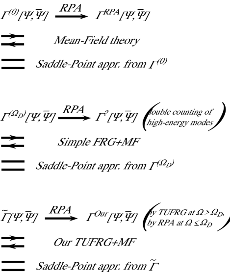
Figure 1: Relationship between the conventional mean-field theory, the simple FRG+MF approach, and our TUFRG+MF approach. A pair of opposite arrows indicates the agreement between their critical conditions, while an equal sign means the physical equivalence.

We can also obtain the result identical to the MF theory within the path-integral formalism, starting from the interaction part $\Gamma^{(0)}[\psi,\bar{\psi}]$ of the action. Namely, introducing, via a Hubbard-Stratonovich transformation, the auxiliary variable associated with superconducting order parameters, and employing the saddle-point approximation, one can arrive at the result that is completely identical to the MF approximation. In this sense, the above three methods can be considered to be physically equivalent. However, the MF theory has an advantage, when compared with the RPA, that it can address the ordered phases of the system.

Now we return to the irreducible action $\tilde{\Gamma}[\psi,\bar{\psi}]$ presented in Eq. (68). In the multichannel RPA, it evolves into $\Gamma^{\Omega_{D}}$ of Eq. (52) at the divergence scale. Namely, the pairing part of the action changes from $\tilde{\Gamma}^{{\rm{sSC}}}+\tilde{\Gamma}^{{\rm{tSC}}}$ of Eq. (68) to $\Gamma^{{\rm{sSC}}}+\Gamma^{{\rm{tSC}}}$ of Eq. (52) in the RPA flow of the pairing channel, while the spin and charge parts transform into $\Gamma^{{\rm{SPN}}}$ and $\Gamma^{{\rm{CHG}}}$, starting from $\tilde{\Gamma}^{{\rm{SPN}}}$ and $\tilde{\Gamma}^{{\rm{CHG}}}$, in the RPA flows of the spin and charge channels, respectively. Moreover, in our approach (using the TUFRG at $\Omega\geq\Omega_{D}$, while using the RPA at $\Omega<\Omega_{D}$), the resulting low-energy-scale action $\Gamma^{\Omega<\Omega_{D}}$ is exactly the same as the one that is obtained by the multichannel RPA starting from $\tilde{\Gamma}$ given in Eq. (68). Taking into account the equivalence between the RPA and MF theory, we arrive at the conclusion that it would be reasonable to choose the interaction Hamiltonian corresponding to $\tilde{\Gamma}[\psi,\bar{\psi}]$ as an input for our mean-field calculation.

Our TUFRG+MF approach is advantageous when compared with the conventional mean-field theory and the simple FRG+MF approach. As a biased method, the mean-field theory neglects the interplay between different channels and emphasize a particular channel. When applied to the case of coexisting orders, the bare interaction should be split into the parts of multiple channels, which leads to an ambiguity in the multichannel MF calculation and may cause a certain bias. In the simple FRG+MF scheme, the resulting effective interaction at the divergence scale, which was obtained by the FRG flow, is directly inserted into the MF calculation. This approach has a drawback that it counts doubly the contributions from high-energy modes and generally overemphasizes the ordering tendencies. The relationship between these three methods is schematically shown in Fig. 1.

III.4 Hubbard-Stratonovich transformation and saddle-point approximation

In the following, we will derive the mean-field equation for our TUFRG+MF approach by resorting to the saddle-point approximation of statistical field theory. Following the discussion in the previous subsection, we use $\tilde{\Gamma}$, instead of $\Gamma^{(0)}$ or $\Gamma^{\Omega_{D}}$, as the interaction part of the action. Therefore, in our TUFRG+MF scheme, we consider the partition function represented as follows:

$$\begin{split}\Xi=&\int{D\bar{\psi}{\kern 1.0pt}D\psi}\exp\{-S_{0}[\psi,\bar{\psi}]-\tilde{\Gamma}[\psi,\bar{\psi}]\}=\int{D\bar{\psi}{\kern 1.0pt}D\psi}\exp\{-S_{0}[\psi,\bar{\psi}]\}\\ &\times\exp\{-\tilde{\Gamma}^{{\rm{sSC}}}[\psi,\bar{\psi}]\}\times\exp\{-\tilde{\Gamma}^{{\rm{tSC}}}[\psi,\bar{\psi}]\}\times\exp\{-\tilde{\Gamma}^{{\rm{SPN}}}[\psi,\bar{\psi}]\}\times\exp\{-\tilde{\Gamma}^{{\rm{CHG}}}[\psi,\bar{\psi}]\},\end{split}$$ (72)

with $S_{0}$ and $\tilde{\Gamma}$ given in Eqs. (3) and (68), respectively. We can use the Hubbard-Stratonovich transformation to decompose the fermionic quartic terms in $\tilde{\Gamma}$ into the fermion bilinears.

For example, let us consider the term containing $\tilde{\Gamma}^{{\rm{sSC}}}$ in Eq. (72). It can be expressed in a factorized form.

$$\begin{split}\exp\{-\tilde{\Gamma}^{{\rm{sSC}}}[\psi,\bar{\psi}]\}=\prod\limits_{i=1}^{N_{\rm{P}}}{\prod\limits_{\alpha={\rm{1}}}^{M_{{\rm{sSC}},i}}{\prod\limits_{\omega}{\exp\left\{{\frac{{\rm{1}}}{2}\frac{1}{{2N\beta\hbar^{2}}}\Lambda^{{\rm{sSC}},\alpha}({\bf{Q}}_{i}^{\rm{P}})[O_{\alpha}^{{\rm{sSC}}}({\bf{Q}}_{i}^{\rm{P}},\omega)]^{*}O_{\alpha}^{{\rm{sSC}}}({\bf{Q}}_{i}^{\rm{P}},\omega)}\right\}}}}\end{split}$$ (73)

We can perform the Hubbard-Stratonovich transformation for each factor of Eq. (73) in the following way:

$$\begin{split}&\exp\left\{{\frac{{\rm{1}}}{2}\frac{1}{{2N\beta\hbar^{2}}}\Lambda^{{\rm{sSC}},\alpha}({\bf{Q}}_{i}^{\rm{P}})[O_{\alpha}^{{\rm{sSC}}}({\bf{Q}}_{i}^{\rm{P}},\omega)]^{*}O_{\alpha}^{{\rm{sSC}}}({\bf{Q}}_{i}^{\rm{P}},\omega)}\right\}=\exp\{\eta[O_{\alpha}^{{\rm{sSC}}}({\bf{Q}}_{i}^{\rm{P}},\omega)]^{*}O_{\alpha}^{{\rm{sSC}}}({\bf{Q}}_{i}^{\rm{P}},\omega)\}\\ &\hskip 144.0pt\times\frac{{\int{d\delta^{*}}\int{d\delta}\exp\left\{{-\frac{1}{\eta}}\right.\left[{\frac{\delta}{\hbar}-\eta O_{\alpha}^{{\rm{sSC}}}({\bf{Q}}_{i}^{\rm{P}},\omega)}\right]^{*}\left.{\left[{\frac{\delta}{\hbar}-\eta O_{\alpha}^{{\rm{sSC}}}({\bf{Q}}_{i}^{\rm{P}},\omega)}\right]}\right\}}}{{\int{d\delta^{*}}\int{d\delta}\exp\left\{{-\frac{1}{\eta}\left({\frac{\delta}{\hbar}}\right)^{*}\left({\frac{\delta}{\hbar}}\right)}\right\}}}\\ &\hskip 24.0pt=\frac{{\int{d\delta^{*}}\int{d\delta}\exp\left\{{-\frac{1}{{\eta\hbar^{2}}}\delta^{*}\delta+\frac{{\delta^{*}}}{\hbar}O_{\alpha}^{{\rm{sSC}}}({\bf{Q}}_{i}^{\rm{P}},\omega)+\frac{\delta}{\hbar}[O_{\alpha}^{{\rm{sSC}}}({\bf{Q}}_{i}^{\rm{P}},\omega)]^{*}}\right\}}}{{\int{d\delta^{*}}\int{d\delta}\exp\left\{{-\frac{1}{{\eta\hbar^{2}}}\delta^{*}\delta}\right\}}}\\ &\hskip 24.0pt=c\int{d\delta^{*}}\int{d\delta}\exp\left\{{-\frac{{4N\beta}}{{\Lambda^{{\rm{sSC}},\alpha}({\bf{Q}}_{i}^{\rm{P}})}}\delta^{*}\delta+\frac{{\delta^{*}}}{\hbar}O_{\alpha}^{{\rm{sSC}}}({\bf{Q}}_{i}^{\rm{P}},\omega)+\frac{\delta}{\hbar}[O_{\alpha}^{{\rm{sSC}}}({\bf{Q}}_{i}^{\rm{P}},\omega)]^{*}}\right\}\end{split}$$

with a complex variable $\delta$, a real constant $c$, and $\eta=\frac{{\Lambda^{{\rm{sSC}},\alpha}({\bf{Q}}_{i}^{\rm{P}})}}{{4N\beta\hbar^{2}}}$. Inserting the above equation into Eq. (73), we obtain the following relation,

$$\begin{split}\exp\left\{-\tilde{\Gamma}^{{\rm{sSC}}}[\psi,\bar{\psi}]\right\}=&C_{{\rm{sSC}}}\int{D\delta_{{\rm{sSC}}}^{*}}\int{D\delta_{{\rm{sSC}}}}\exp\left\{{-S_{{\rm{HS}}}^{{\rm{sSC}}}[\psi,\bar{\psi};\delta_{{\rm{sSC}}}^{*},\delta_{{\rm{sSC}}}]}\right\},\\ S_{{\rm{HS}}}^{{\rm{sSC}}}[\psi,\bar{\psi};\delta_{{\rm{sSC}}}^{*},\delta_{{\rm{sSC}}}]\equiv&\sum\limits_{i=1}^{N_{\rm{P}}}{\sum\limits_{\alpha=1}^{M_{{\rm{sSC}},i}}{\sum\limits_{\omega}{\left\{{\frac{{4N\beta}}{{\Lambda^{{\rm{sSC}},\alpha}({\bf{Q}}_{i}^{\rm{P}})}}}\right.[\delta_{\alpha}^{{\rm{sSC}}}({\bf{Q}}_{i}^{\rm{P}},\omega)]^{*}\delta_{\alpha}^{{\rm{sSC}}}({\bf{Q}}_{i}^{\rm{P}},\omega)}}}\\ &-\frac{1}{\hbar}[\delta_{\alpha}^{{\rm{sSC}}}({\bf{Q}}_{i}^{\rm{P}},\omega)]^{*}O_{\alpha}^{{\rm{sSC}}}({\bf{Q}}_{i}^{\rm{P}},\omega)-\left.{\frac{1}{\hbar}\delta_{\alpha}^{{\rm{sSC}}}({\bf{Q}}_{i}^{\rm{P}},\omega)[O_{\alpha}^{{\rm{sSC}}}({\bf{Q}}_{i}^{\rm{P}},\omega)]^{*}}\right\}.\end{split}$$ (74)

In a similar way, after a tedious calculation, we derive the following equations:

$$\begin{split}\exp\left\{-\tilde{\Gamma}^{{\rm{tSC}}}[\psi,\bar{\psi}]\right\}=&C_{{\rm{tSC}}}\int{D\vec{\delta}_{{\rm{tSC}}}^{*}}\int{D\vec{\delta}_{{\rm{tSC}}}}\exp\left\{{-S_{{\rm{HS}}}^{{\rm{tSC}}}[\psi,\bar{\psi};\vec{\delta}_{{\rm{tSC}}}^{*},\vec{\delta}_{{\rm{tSC}}}]}\right\},\\ S_{{\rm{HS}}}^{{\rm{tSC}}}[\psi,\bar{\psi};\vec{\delta}_{{\rm{tSC}}}^{*},\vec{\delta}_{{\rm{tSC}}}]\equiv&\sum\limits_{i=1}^{N_{\rm{P}}}{\sum\limits_{\alpha=1}^{M_{{\rm{tSC}},i}}{\sum\limits_{\omega}{\left\{{\frac{{4N\beta}}{{\Lambda^{{\rm{tSC}},\alpha}({\bf{Q}}_{i}^{\rm{P}})}}}\right.[\vec{\delta}_{\alpha}^{{\rm{tSC}}}({\bf{Q}}_{i}^{\rm{P}},\omega)]^{*}\cdot\vec{\delta}_{\alpha}^{{\rm{tSC}}}({\bf{Q}}_{i}^{\rm{P}},\omega)}}}\\ &-\frac{1}{\hbar}[\vec{\delta}_{\alpha}^{{\rm{tSC}}}({\bf{Q}}_{i}^{\rm{P}},\omega)]^{*}\cdot\vec{O}_{\alpha}^{{\rm{tSC}}}({\bf{Q}}_{i}^{\rm{P}},\omega)-\left.{\frac{1}{\hbar}\vec{\delta}_{\alpha}^{{\rm{tSC}}}({\bf{Q}}_{i}^{\rm{P}},\omega)\cdot[\vec{O}_{\alpha}^{{\rm{tSC}}}({\bf{Q}}_{i}^{\rm{P}},\omega)]^{*}}\right\},\end{split}$$ (75)

$$\begin{split}\exp\left\{-\tilde{\Gamma}^{{\rm{SPN}}}[\psi,\bar{\psi}]\right\}=&C_{{\rm{SPN}}}\int{D\vec{\delta}_{{\rm{SPN}}}^{*}}\int{D\vec{\delta}_{{\rm{SPN}}}}\exp\left\{-S_{{\rm{HS}}}^{{\rm{SPN}}}[\psi,\bar{\psi};\vec{\delta}_{{\rm{SPN}}}^{*},\vec{\delta}_{{\rm{SPN}}}]\right\},\\ S_{{\rm{HS}}}^{{\rm{SPN}}}[\psi,\bar{\psi};\vec{\delta}_{{\rm{SPN}}}^{*},\vec{\delta}_{{\rm{SPN}}}]\equiv&\sum\limits_{i=1}^{N_{\rm{C}}}{\sum\limits_{\alpha=1}^{M_{{\rm{C}},i}}{\sum\limits_{\omega}{\left\{{\frac{{4N\beta}}{{\Lambda^{{\rm{C}},\alpha}({\bf{Q}}_{i}^{\rm{C}})}}}\right.[\vec{\delta}_{\alpha}^{{\rm{SPN}}}({\bf{Q}}_{i}^{\rm{C}},\omega)]^{*}\cdot\vec{\delta}_{\alpha}^{{\rm{SPN}}}({\bf{Q}}_{i}^{\rm{C}},\omega)}}}\\ &-\frac{1}{\hbar}[\vec{\delta}_{\alpha}^{{\rm{SPN}}}({\bf{Q}}_{i}^{\rm{C}},\omega)]^{*}\cdot\vec{O}_{\alpha}^{{\rm{SPN}}}({\bf{Q}}_{i}^{\rm{C}},\omega)-\left.{\frac{1}{\hbar}\vec{\delta}_{\alpha}^{{\rm{SPN}}}({\bf{Q}}_{i}^{\rm{C}},\omega)\cdot[\vec{O}_{\alpha}^{{\rm{SPN}}}({\bf{Q}}_{i}^{\rm{C}},\omega)]^{*}}\right\},\\ \textrm{ with a constraint }&\vec{\delta}_{\alpha}^{{\rm{SPN}}}({\bf{Q}}_{i}^{\rm{C}},\omega)=[\vec{\delta}_{\alpha}^{{\rm{SPN}}}(-{\bf{Q}}_{i}^{\rm{C}},-\omega)]^{*},\end{split}$$ (76)

$$\begin{split}\exp\left\{-\tilde{\Gamma}^{{\rm{CHG}}}[\psi,\bar{\psi}]\right\}=&C_{{\rm{CHG}}}\int{D\delta_{{\rm{CHG}}}^{*}}\int{D\delta_{{\rm{CHG}}}}\exp\left\{-S_{{\rm{HS}}}^{{\rm{CHG}}}[\psi,\bar{\psi};\delta_{{\rm{CHG}}}^{*},\delta_{{\rm{CHG}}}]\right\},\\ S_{{\rm{HS}}}^{{\rm{CHG}}}[\psi,\bar{\psi};\delta_{{\rm{CHG}}}^{*},\delta_{{\rm{CHG}}}]\equiv&\sum\limits_{i=1}^{N_{\rm{W}}}{\sum\limits_{\alpha=1}^{M_{{\rm{W}},i}}{\sum\limits_{\omega}{\left\{{\frac{{4N\beta}}{{\Lambda^{{\rm{W}},\alpha}({\bf{Q}}_{i}^{\rm{W}})}}}\right.[\delta_{\alpha}^{{\rm{CHG}}}({\bf{Q}}_{i}^{\rm{W}},\omega)]^{*}\delta_{\alpha}^{{\rm{CHG}}}({\bf{Q}}_{i}^{\rm{W}},\omega)}}}\\ &-\frac{1}{\hbar}[\delta_{\alpha}^{{\rm{CHG}}}({\bf{Q}}_{i}^{\rm{W}},\omega)]^{*}O_{\alpha}^{{\rm{CHG}}}({\bf{Q}}_{i}^{\rm{W}},\omega)-\left.{\frac{1}{\hbar}\delta_{\alpha}^{{\rm{CHG}}}({\bf{Q}}_{i}^{\rm{W}},\omega)[O_{\alpha}^{{\rm{CHG}}}({\bf{Q}}_{i}^{\rm{W}},\omega)]^{*}}\right\},\\ \textrm{ with a constraint }&\delta_{\alpha}^{{\rm{CHG}}}({\bf{Q}}_{i}^{\rm{W}},\omega)=[\delta_{\alpha}^{{\rm{CHG}}}(-{\bf{Q}}_{i}^{\rm{W}},-\omega)]^{*}.\end{split}$$ (77)

Near the critical points, the electronic instabilities are dominated by $\omega=0$ components of the auxiliary variables $\delta_{\alpha}^{\rm{X}}({\bf{Q}},\omega)$ (for a detailed discussion, see pages 89–91 of Ref. [Nagaosa, 1999]). Therefore, in what follows we will only consider these components and eliminate the $\omega$-dependence of $\delta_{\alpha}^{\rm{X}}({\bf{Q}},\omega)$ and $O_{\alpha}^{\rm{X}}({\bf{Q}},\omega)$, with implicit definition of $\delta_{\alpha}^{\rm{X}}({\bf{Q}})\equiv\delta_{\alpha}^{\rm{X}}({\bf{Q}},\omega=0)$ and $O_{\alpha}^{\rm{X}}({\bf{Q}})\equiv O_{\alpha}^{\rm{X}}({\bf{Q}},\omega=0)$.

Inserting Eqs. (74)–(77) into Eq. (72), we have

$$\begin{split}\Xi=&C\int{D\{\delta^{*}\}}\int{D\{\delta\}}\left({\int{D\bar{\psi}{\kern 1.0pt}D\psi}\exp\left\{-S_{0}[\psi,\bar{\psi}]-S_{{\rm{HS}}}[\psi,\bar{\psi};\{\delta^{*}\},\{\delta\}]\right\}}\right)\\ =&C\int{D\{\delta^{*}\}}\int{D\{\delta\}}\exp\left\{-\beta\Omega^{{\rm{HS}}}[\{\delta^{*}\},\{\delta\}]\right\},\end{split}$$ (78)

with the definition of

$$\begin{split}S_{{\rm{HS}}}[\psi,\bar{\psi};\{\delta^{*}\},\{\delta\}]\equiv&S_{{\rm{HS}}}^{{\rm{sSC}}}[\psi,\bar{\psi};\delta_{{\rm{sSC}}}^{*},\delta_{{\rm{sSC}}}]+S_{{\rm{HS}}}^{{\rm{tSC}}}[\psi,\bar{\psi};\vec{\delta}_{{\rm{tSC}}}^{*},\vec{\delta}_{{\rm{tSC}}}]\\ &+S_{{\rm{HS}}}^{{\rm{SPN}}}[\psi,\bar{\psi};\vec{\delta}_{{\rm{SPN}}}^{*},\vec{\delta}_{{\rm{SPN}}}]+S_{{\rm{HS}}}^{{\rm{CHG}}}[\psi,\bar{\psi};\delta_{{\rm{CHG}}}^{*},\delta_{{\rm{CHG}}}]\},\end{split}$$ (79)

$$\begin{split}\Omega^{{\rm{HS}}}[\{\delta^{*}\},\{\delta\}]\equiv-\frac{1}{\beta}\ln\left({\int{D\bar{\psi}{\kern 1.0pt}D\psi}\exp\left\{{-S_{0}[\psi,\bar{\psi}]-S_{{\rm{HS}}}[\psi,\bar{\psi};\{\delta^{*}\},\{\delta\}]}\right\}}\right),\end{split}$$ (80)

and with an abbreviation $\{\delta\}\equiv(\delta_{{\rm{sSC}}},\vec{\delta}_{{\rm{tSC}}},\vec{\delta}_{{\rm{SPN}}},\delta_{{\rm{CHG}}})$. Equation (78) indicates that the probability of the auxiliary variables to take the values $(\delta_{{\rm{sSC}}},\vec{\delta}_{{\rm{tSC}}},\vec{\delta}_{{\rm{SPN}}},\delta_{{\rm{CHG}}})$ is proportional to $e^{-\beta\Omega^{{\rm{HS}}}[\{\delta^{*}\},\{\delta\}]}$. Therefore, the value of $\{\delta\}$ with the maximal provability corresponds to the minimum of the Hubbard-Stratonovich thermodynamic potential $\Omega^{{\rm{HS}}}[\{\delta^{*}\},\{\delta\}]$.

In the integration of Eq. (78), one usually employs the saddle-point approximation. Within this approximation the result of the integration is approximated to be the maximal value of the integrand. Namely, the saddle-point approximation is represented as

$$\begin{split}\Xi\approx\exp\left\{-\beta\Omega^{{\rm{HS}}}[\{\Delta^{*}\},\{\Delta\}]\right\}=\int{D\bar{\psi}D\psi}\exp\left\{-S_{0}[\psi,\bar{\psi}]-S_{{\rm{HS}}}[\psi,\bar{\psi};\{\Delta^{*}\},\{\Delta\}]\right\}.\end{split}$$ (81)

Here the mean-field parameters $\{\Delta\}\equiv(\Delta_{{\rm{sSC}}},\vec{\Delta}_{{\rm{tSC}}},\vec{\Delta}_{{\rm{SPN}}},\Delta_{{\rm{CHG}}})$ are determined by the minimization of the effective thermodynamic potential:

$$\begin{split}\Omega^{{\rm{HS}}}[\{\Delta^{*}\},\{\Delta\}]=\min\left\{{\Omega^{{\rm{HS}}}[\{\delta^{*}\},\{\delta\}]}\right\}.\end{split}$$ (82)

Equation (81) implies that the interacting system in the saddle-point approximation turns into the noninteracting system in the external field determined by the parameters $\{\Delta\}$. Combining the minimization condition (82) and Eq. (80), we obtain the following self-consistency condition:

$$\begin{split}\Delta_{\alpha}^{{\rm{sSC}}}({\bf{Q}}_{i}^{\rm{P}})=&\frac{{\Lambda^{{\rm{sSC}},\alpha}({\bf{Q}}_{i}^{\rm{P}})}}{{4N\beta\hbar}}\left\langle{O_{\alpha}^{{\rm{sSC}}}({\bf{Q}}_{i}^{\rm{P}})}\right\rangle_{\Delta},\vec{\Delta}_{\alpha}^{{\rm{tSC}}}({\bf{Q}}_{i}^{\rm{P}})=\frac{{\Lambda^{{\rm{tSC}},\alpha}({\bf{Q}}_{i}^{\rm{P}})}}{{4N\beta\hbar}}\left\langle{\vec{O}_{\alpha}^{{\rm{tSC}}}({\bf{Q}}_{i}^{\rm{P}})}\right\rangle_{\Delta},\\ \vec{\Delta}_{\alpha}^{{\rm{SPN}}}({\bf{Q}}_{i}^{\rm{C}})=&\frac{{\Lambda^{{\rm{C}},\alpha}({\bf{Q}}_{i}^{\rm{C}})}}{{4N\beta\hbar}}\left\langle{\vec{O}_{\alpha}^{{\rm{SPN}}}({\bf{Q}}_{i}^{\rm{C}})}\right\rangle_{\Delta},\Delta_{\alpha}^{{\rm{CHG}}}({\bf{Q}}_{i}^{\rm{W}})=\frac{{\Lambda^{{\rm{W}},\alpha}({\bf{Q}}_{i}^{\rm{W}})}}{{4N\beta\hbar}}\left\langle{O_{\alpha}^{{\rm{CHG}}}({\bf{Q}}_{i}^{\rm{W}})}\right\rangle_{\Delta},\end{split}$$ (83)

with the mean value defined by

$$\begin{split}\left\langle A\right\rangle_{\Delta}\equiv\frac{{\int{D\bar{\psi}{\kern 1.0pt}D\psi}\exp\left\{-S_{0}[\psi,\bar{\psi}]-S_{{\rm{HS}}}[\psi,\bar{\psi};\{\Delta^{*}\},\{\Delta\}]\right\}A}}{{\int{D\bar{\psi}{\kern 1.0pt}D\psi}\exp\left\{-S_{0}[\psi,\bar{\psi}]-S_{{\rm{HS}}}[\psi,\bar{\psi};\{\Delta^{*}\},\{\Delta\}]\right\}}}.\end{split}$$ (84)

Thus, in the saddle-point approximation, the system is described by the approximate action:

$$\begin{split}S_{{\rm{MF}}}=S_{0}[\psi,\bar{\psi}]+S_{{\rm{HS}}}[\psi,\bar{\psi};\{\Delta^{*}\},\{\Delta\}]\end{split}$$ (85)

with $S_{0}$ and $S_{{\rm{HS}}}$, represented by Eqs. (3) and (79), respectively.

Now we return to the operator formalism. The action (85) is equivalent to the following mean-field Hamiltonian:

$$\begin{split}&\hat{H}_{{\rm{MF}}}=\hat{H}_{0}+\hat{H}_{{\rm{sSC}}}+\hat{H}_{{\rm{tSC}}}+\hat{H}_{{\rm{SPN}}}+\hat{H}_{{\rm{CHG}}},\hat{H}_{0}=\sum\limits_{o,o^{\prime}}{\sum\limits_{{\bf{k}},\sigma}{\hat{c}_{{\bf{k}}o\sigma}^{\dagger}(H_{oo^{\prime}}^{0}({\bf{k}})-\mu\delta_{oo^{\prime}})\hat{c}_{{\bf{k}}o^{\prime}\sigma}}},\\ &\hat{H}_{{\rm{sSC}}}=\sum\limits_{i=1}^{N_{\rm{P}}}{\sum\limits_{\alpha=1}^{M_{{\rm{sSC}},i}}{\left({\frac{{4N}}{{\Lambda^{{\rm{sSC}},\alpha}({\bf{Q}}_{i}^{\rm{P}})}}[\Delta_{\alpha}^{{\rm{sSC}}}({\bf{Q}}_{i}^{\rm{P}})]^{*}\Delta_{\alpha}^{{\rm{sSC}}}({\bf{Q}}_{i}^{\rm{P}})-[\Delta_{\alpha}^{{\rm{sSC}}}({\bf{Q}}_{i}^{\rm{P}})]^{*}\hat{O}_{\alpha}^{{\rm{sSC}}}({\bf{Q}}_{i}^{\rm{P}})-\Delta_{\alpha}^{{\rm{sSC}}}({\bf{Q}}_{i}^{\rm{P}})[\hat{O}_{\alpha}^{{\rm{sSC}}}({\bf{Q}}_{i}^{\rm{P}})]^{\dagger}}\right)}},\\ &\hat{H}_{{\rm{tSC}}}=\sum\limits_{i=1}^{N_{\rm{P}}}{\sum\limits_{\alpha=1}^{M_{{\rm{tSC}},i}}{\left({\frac{{4N}}{{\Lambda^{{\rm{tSC}},\alpha}({\bf{Q}}_{i}^{\rm{P}})}}[\vec{\Delta}_{\alpha}^{{\rm{tSC}}}({\bf{Q}}_{i}^{\rm{P}})]^{*}\cdot\vec{\Delta}_{\alpha}^{{\rm{tSC}}}({\bf{Q}}_{i}^{\rm{P}})-[\vec{\Delta}_{\alpha}^{{\rm{tSC}}}({\bf{Q}}_{i}^{\rm{P}})]^{*}\cdot\hat{\vec{O}}_{\alpha}^{{\rm{tSC}}}({\bf{Q}}_{i}^{\rm{P}})-\vec{\Delta}_{\alpha}^{{\rm{tSC}}}({\bf{Q}}_{i}^{\rm{P}})\cdot[\hat{\vec{O}}_{\alpha}^{{\rm{tSC}}}({\bf{Q}}_{i}^{\rm{P}})]^{\dagger}}\right)}},\\ &\hat{H}_{{\rm{SPN}}}=\sum\limits_{i=1}^{N_{\rm{C}}}{\sum\limits_{\alpha=1}^{M_{{\rm{C}},i}}{\left({\frac{{4N}}{{\Lambda^{{\rm{C}},\alpha}({\bf{Q}}_{i}^{\rm{C}})}}[\vec{\Delta}_{\alpha}^{{\rm{SPN}}}({\bf{Q}}_{i}^{\rm{C}},\omega)]^{*}\cdot\vec{\Delta}_{\alpha}^{{\rm{SPN}}}({\bf{Q}}_{i}^{\rm{C}},\omega)-[\vec{\Delta}_{\alpha}^{{\rm{SPN}}}({\bf{Q}}_{i}^{\rm{C}})]^{*}\cdot\hat{\vec{O}}_{\alpha}^{{\rm{SPN}}}({\bf{Q}}_{i}^{\rm{C}})-\vec{\Delta}_{\alpha}^{{\rm{SPN}}}({\bf{Q}}_{i}^{\rm{C}})\cdot[\hat{\vec{O}}_{\alpha}^{{\rm{SPN}}}({\bf{Q}}_{i}^{\rm{C}})]^{\dagger}}\right)}},\\ &\hat{H}_{{\rm{CHG}}}=\sum\limits_{i=1}^{N_{\rm{W}}}{\sum\limits_{\alpha=1}^{M_{{\rm{W}},i}}{\left({\frac{{4N}}{{\Lambda^{{\rm{W}},\alpha}({\bf{Q}}_{i}^{\rm{W}})}}[\Delta_{\alpha}^{{\rm{CHG}}}({\bf{Q}}_{i}^{\rm{W}})]^{*}\Delta_{\alpha}^{{\rm{CHG}}}({\bf{Q}}_{i}^{\rm{W}})-[\Delta_{\alpha}^{{\rm{CHG}}}({\bf{Q}}_{i}^{\rm{W}})]^{*}[\hat{\vec{O}}_{\alpha}^{{\rm{CHG}}}({\bf{Q}}_{i}^{\rm{W}})-\Delta_{\alpha}^{{\rm{CHG}}}({\bf{Q}}_{i}^{\rm{W}})[\hat{\vec{O}}_{\alpha}^{{\rm{CHG}}}({\bf{Q}}_{i}^{\rm{W}})]^{\dagger}}\right)}},\\ &\hskip 24.0pt\textrm{ with constraints }\vec{\Delta}_{\alpha}^{{\rm{SPN}}}({\bf{Q}}_{i}^{\rm{C}})=[\vec{\Delta}_{\alpha}^{{\rm{SPN}}}(-{\bf{Q}}_{i}^{\rm{C}})]^{*},\Delta_{\alpha}^{{\rm{CHG}}}({\bf{Q}}_{i}^{\rm{W}})=[\Delta_{\alpha}^{{\rm{CHG}}}(-{\bf{Q}}_{i}^{\rm{W}})]^{*}.\end{split}$$ (86)

Here the operators $\hat{O}_{\alpha}^{\rm{X}}$ are expressed as

$$\begin{split}\hat{O}_{\alpha}^{{\rm{sSC}}}({\bf{Q}}_{i}^{\rm{P}})=&\sum\limits_{\bf{k}}{\sum\limits_{o,o^{\prime},m}{[\varphi_{oo^{\prime}m}^{{\rm{P}},\alpha}({\bf{Q}}_{i}^{\rm{P}})]^{*}e^{i{\bf{R}}_{m}\cdot{\bf{k}}}}}\sum\limits_{\sigma}{\sigma\hat{c}_{-{\bf{k}},o^{\prime},-\sigma}\hat{c}_{{\bf{k}}+{\bf{Q}}_{i}^{\rm{P}},o,\sigma}},\\ \hat{\vec{O}}_{\alpha}^{{\rm{tSC}}}({\bf{Q}}_{i}^{\rm{P}})=&(\hat{O}_{\alpha,x}^{{\rm{tSC}}}({\bf{Q}}_{i}^{\rm{P}}),\hat{O}_{\alpha,y}^{{\rm{tSC}}}({\bf{Q}}_{i}^{\rm{P}}),\hat{O}_{\alpha,z}^{{\rm{tSC}}}({\bf{Q}}_{i}^{\rm{P}}))=\sum\limits_{\bf{k}}{\sum\limits_{o,o^{\prime},m}{[\varphi_{oo^{\prime}m}^{{\rm{P}},\alpha}({\bf{Q}}_{i}^{\rm{P}})]^{*}e^{i{\bf{R}}_{m}\cdot{\bf{k}}}}}\\ &\times\left.{\left({-\sum\limits_{\sigma}{\sigma\hat{c}_{-{\bf{k}},o^{\prime},\sigma}\hat{c}_{{\bf{k}}+{\bf{Q}}_{i}^{\rm{P}},o,\sigma}},}\right.-i\sum\limits_{\sigma}{\hat{c}_{-{\bf{k}},o^{\prime},\sigma}\hat{c}_{{\bf{k}}+{\bf{Q}}_{i}^{\rm{P}},o,\sigma}},\sum\limits_{\sigma}{\hat{c}_{-{\bf{k}},o^{\prime},-\sigma}\hat{c}_{{\bf{k}}+{\bf{Q}}_{i}^{\rm{P}},o,\sigma}}}\right),\\ \hat{\vec{O}}_{\alpha}^{{\rm{SPN}}}({\bf{Q}}_{i}^{\rm{C}})=&\sum\limits_{\bf{k}}{\sum\limits_{o,o^{\prime},m}{[\varphi_{oo^{\prime}m}^{{\rm{C}},\alpha}({\bf{Q}}_{i}^{\rm{C}})]^{*}e^{i{\bf{R}}_{m}\cdot{\bf{k}}}}}\sum\limits_{\sigma,\sigma^{\prime}}{\hat{c}_{{\bf{k}},o^{\prime},\sigma}^{\dagger}\vec{\sigma}_{\sigma\sigma^{\prime}}\hat{c}_{{\bf{k}}+{\bf{Q}}_{i}^{\rm{C}},o,\sigma^{\prime}}},\\ \hat{O}_{\alpha}^{{\rm{CHG}}}({\bf{Q}}_{i}^{\rm{W}})=&\sum\limits_{\bf{k}}{\sum\limits_{o,o^{\prime},m}{[\varphi_{oo^{\prime}m}^{{\rm{W}},\alpha}({\bf{Q}}_{i}^{\rm{W}})]^{*}e^{i{\bf{R}}_{m}\cdot{\bf{k}}}}}\sum\limits_{\sigma}{\hat{c}_{{\bf{k}},o^{\prime},\sigma}^{\dagger}\hat{c}_{{\bf{k}}+{\bf{Q}}_{i}^{\rm{W}},o,\sigma}},\end{split}$$ (87)

with the symmetry relation

$$\begin{split}\hat{\vec{O}}_{\alpha}^{{\rm{SPN}}}(-{\bf{Q}}_{i}^{\rm{C}})=[\hat{\vec{O}}_{\alpha}^{{\rm{SPN}}}({\bf{Q}}_{i}^{\rm{C}})]^{\dagger},\hat{O}_{\alpha}^{{\rm{CHG}}}(-{\bf{Q}}_{i}^{\rm{W}})=[\hat{O}_{\alpha}^{{\rm{CHG}}}({\bf{Q}}_{i}^{\rm{W}})]^{\dagger}.\end{split}$$ (88)

In addition, inserting the relations,

$$\begin{split}&\frac{1}{{\beta\hbar}}\left\langle{\sum\limits_{\omega}{\bar{\psi}(\alpha,\omega)\psi(\beta,\omega)}}\right\rangle_{\Delta}=\left\langle{\hat{c}_{\alpha}^{\dagger}\hat{c}_{\beta}}\right\rangle_{{\rm{MF}}},\\ &\frac{1}{{\beta\hbar}}\left\langle{\sum\limits_{\omega}{\psi(\alpha,\omega)\psi(\beta,-\omega)}}\right\rangle_{\Delta}=\left\langle{\hat{c}_{\alpha}\hat{c}_{\beta}}\right\rangle_{{\rm{MF}}},\frac{1}{{\beta\hbar}}\left\langle{\sum\limits_{\omega}{\bar{\psi}(\alpha,\omega)\bar{\psi}(\beta,-\omega)}}\right\rangle_{\Delta}=\left\langle{\hat{c}_{\alpha}^{\dagger}\hat{c}_{\beta}^{\dagger}}\right\rangle_{{\rm{MF}}},\end{split}$$

into Eq. (83), we have the self-consistency condition in the operator formalism:

$$\begin{split}\Delta_{\alpha}^{{\rm{sSC}}}({\bf{Q}}_{i}^{\rm{P}})=&\frac{{\Lambda^{{\rm{sSC}},\alpha}({\bf{Q}}_{i}^{\rm{P}})}}{{4N}}\left\langle{\hat{O}_{\alpha}^{{\rm{sSC}}}({\bf{Q}}_{i}^{\rm{P}})}\right\rangle_{{\rm{MF}}},\vec{\Delta}_{\alpha}^{{\rm{tSC}}}({\bf{Q}}_{i}^{\rm{P}})=\frac{{\Lambda^{{\rm{tSC}},\alpha}({\bf{Q}}_{i}^{\rm{P}})}}{{4N}}\left\langle{\hat{\vec{O}}_{\alpha}^{{\rm{tSC}}}({\bf{Q}}_{i}^{\rm{P}})}\right\rangle_{{\rm{MF}}},\\ \vec{\Delta}_{\alpha}^{{\rm{SPN}}}({\bf{Q}}_{i}^{\rm{C}})=&\frac{{\Lambda^{{\rm{C}},\alpha}({\bf{Q}}_{i}^{\rm{C}})}}{{4N}}\left\langle{\hat{\vec{O}}_{\alpha}^{{\rm{SPN}}}({\bf{Q}}_{i}^{\rm{C}})}\right\rangle_{{\rm{MF}}},\Delta_{\alpha}^{{\rm{CHG}}}({\bf{Q}}_{i}^{\rm{W}})=\frac{{\Lambda^{{\rm{W}},\alpha}({\bf{Q}}_{i}^{\rm{W}})}}{{4N}}\left\langle{\hat{O}_{\alpha}^{{\rm{CHG}}}({\bf{Q}}_{i}^{\rm{W}})}\right\rangle_{{\rm{MF}}}.\end{split}$$ (89)

Here $\left\langle{\hat{A}}\right\rangle_{{\rm{MF}}}$ is the mean value of the operator $\hat{A}$ of the system described by $\hat{H}_{{\rm{MF}}}$, in the grand canonical ensemble.

At zero temperature the minimization condition of Eq. (82) translates into the minimization of the ground-state energy for the mean-field Hamiltonian (86). At the same time, the self-consistency condition (89) will also coincide with the minimization condition of the ground-state energy.

IV Coexistence phase of chiral SC and chiral SDW

This section presents the first application of our TUFRG+MF approach to competing or coexisting orders. Actually, our approach has already been applied, with poor elucidation and derivation, to the simple case with a unique singular mode in the spin channel An et al. (2023). Very similar scheme has been used in the context of the singular-mode FRG to determine the superconducting gap of strontium ruthenate Wang et al. (2019), but without any derivation and justification. In this section, we use our TUFRG+MF approach to analyze competing chiral $d$-wave SC Nandkishore et al. (2012); Kiesel et al. (2012); Gu et al. (2013); Ying and Wessel (2018) and chiral SDW Ying and Wessel (2018); Li (2012); Jiang et al. (2014) orders which have been predicted to be possible in graphene near van Hove filling. In some FRG studies Wang et al. (2012); O et al. (2021), it was concluded that the chiral SDW phase is generated right around van Hove filling, while the chiral $d$-wave SC emerges slightly away from it. Here we will focus our attention on the value of both order parameters, $\Delta_{d_{1,2}}^{{\rm{sSC}}}({\bf{Q}}=0)$ and $\vec{\Delta}^{{\rm{SPN}}}({\bf{Q}}={\bf{M}}_{1,2,3})$, as a function of doping. In the following we will denote these parameters as $\Delta_{1,2}^{{\rm{sSC}}}=\Delta_{d_{1,2}}^{{\rm{sSC}}}({\bf{Q}}=0)$ and $\vec{\Delta}^{{\rm{SPN}}}({\bf{M}}_{1,2,3})=\vec{\Delta}^{{\rm{SPN}}}({\bf{Q}}={\bf{M}}_{1,2,3})$.

We study the Hubbard model on the honeycomb lattice doped close to van Hove filling.

$$\begin{split}\hat{H}=&\hat{H}_{0}+\hat{H}_{{\mathop{\rm int}}},\\ \hat{H}_{0}=&-t\sum\limits_{\left\langle{iA,jB}\right\rangle,\sigma}{(\hat{c}_{iA\sigma}^{\dagger}\hat{c}_{jB\sigma}}+{\rm{H}}{\rm{.c}}{\rm{.}})\end{split}$$

$$\begin{split}&-t^{\prime}\sum\limits_{\left\langle{\left\langle{io,jo}\right\rangle}\right\rangle,o,\sigma}{(\hat{c}_{io\sigma}^{\dagger}\hat{c}_{jo\sigma}}+{\rm{H}}{\rm{.c}}{\rm{.}})-\mu\sum\limits_{i,o,\sigma}{\hat{c}_{io\sigma}^{\dagger}\hat{c}_{io\sigma}},\\ \hat{H}_{{\mathop{\rm int}}}=&U\sum\limits_{i,0}{\hat{n}_{io\uparrow}\hat{n}_{io\downarrow}}.\end{split}$$ (90)

Here $t$ and $t^{\prime}$ are the hopping amplitudes between nearest and next-nearest neighbors, $\mu$ is the chemical potential, while $\left\langle{iA,jB}\right\rangle$ and $\left\langle{\left\langle{io,jo}\right\rangle}\right\rangle$ denote nearest-neighbor and next-nearest-neighbor bonds. The doping level is defined by $\delta=n_{e}-1$ with $n_{e}$ being the number of electrons per site. The chemical potential and the doping level have the values of $\mu_{{\rm{VH}}}=t+2t^{\prime},\delta_{{\rm{VH}}}=0.25$ at Van Hove filling. We set the parameters as $t=2.8{\rm{eV}},t^{\prime}=0.1{\rm{eV}},U=10.08{\rm{eV}}$, which were used in our previous work O et al. (2021). We investigate the range of doping corresponding to $n_{e}=1.25-1.29$. Figure 2 shows the Brillouin zone (BZ) of the honeycomb lattice and sampling points for transfer momenta within the irreducible region of BZ.

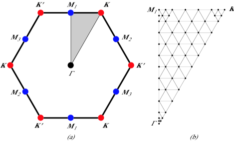
Figure 2: (a) Brillouin zone and high-symmetry points of the honeycomb lattice. The gray triangle is the irreducible region of the Brillouin zone. (b) Mesh of sampling points for transfer momenta within the irreducible region. Only the bosonic propagators with these transfer momenta are numerically calculated at each step of the TUFRG, while others are generated by using the point-group symmetry relations O et al. (2019, 2021).

For the parameter sets considered in the present work, the chiral $d$-wave SC and the chiral SDW constitute main ingredients of the resulting phase diagram. Following the process given in Sec. III.2, the irreducible coupling constants and singular modes are extracted from the bosonic propagators in the pairing and spin channels that were obtained by the TUFRG flow. Then we perform the mean-field calculation, with these coupling constants and singular modes, following the procedure described in Sec. III.4. At this stage the system is depicted by the following mean-field Hamiltonian:

$$\begin{split}\hat{H}_{{\rm{MF}}}=&\hat{H}_{0}+\hat{H}_{{\rm{sSC}}}+\hat{H}_{{\rm{SPN}}},\\ \hat{H}_{0}=&\sum\limits_{{\bf{k}},\sigma}{\left\{{[-tF({\bf{k}})]\hat{c}_{{\bf{k}}A\sigma}^{\dagger}\hat{c}_{{\bf{k}}B\sigma}}\right.}\\ &+\left.{[-tF^{*}({\bf{k}})]\hat{c}_{{\bf{k}}B\sigma}^{\dagger}\hat{c}_{{\bf{k}}A\sigma}}\right\}\\ &+\sum\limits_{{\bf{k}},o,\sigma}{[-t^{\prime}g({\bf{k}})-\mu]\hat{c}_{{\bf{k}}o\sigma}^{\dagger}\hat{c}_{{\bf{k}}o\sigma}},\\ \hat{H}_{{\rm{sSC}}}=&\sum\limits_{\alpha=1,2}{\left({\frac{{4N}}{{\Lambda^{{\rm{sSC}}}}}}\right.}(\Delta_{\alpha}^{{\rm{sSC}}})^{*}\Delta_{\alpha}^{{\rm{sSC}}}\\ &\left.{-(\Delta_{\alpha}^{{\rm{sSC}}})^{*}\hat{O}_{\alpha}^{{\rm{sSC}}}-\Delta_{\alpha}^{{\rm{sSC}}}(\hat{O}_{\alpha}^{{\rm{sSC}}})^{\dagger}}\right)\\ =&\sum\limits_{\alpha=1,2}{\left({\frac{{4N}}{{\Lambda^{{\rm{sSC}}}}}(\Delta_{\alpha}^{{\rm{sSC}}})^{*}\Delta_{\alpha}^{{\rm{sSC}}}}\right.}\\ &-\sum\limits_{\bf{k}}{\sum\limits_{o,o^{\prime},m}{(\varphi_{oo^{\prime}m}^{{\rm{sSC}},\alpha})^{*}e^{i{\bf{R}}_{m}\cdot{\bf{k}}}}}\\ &\times(\Delta_{\alpha}^{{\rm{sSC}}})^{*}\sum\limits_{\sigma}{\sigma\hat{c}_{-{\bf{k}},o^{\prime},-\sigma}\hat{c}_{{\bf{k}},o,\sigma}}\\ &-\sum\limits_{\bf{k}}{\sum\limits_{o,o^{\prime},m}{\varphi_{oo^{\prime}m}^{{\rm{sSC}},\alpha}e^{-i{\bf{R}}_{m}\cdot{\bf{k}}}}}\\ &\times\left.{\Delta_{\alpha}^{{\rm{sSC}}}\sum\limits_{\sigma}{\sigma\hat{c}_{{\bf{k}},o,\sigma}^{\dagger}\hat{c}_{-{\bf{k}},o^{\prime},-\sigma}^{\dagger}}}\right),\\ \hat{H}_{{\rm{SPN}}}=&\sum\limits_{i=1}^{3}{\left({\frac{{4N}}{{\Lambda^{\rm{C}}}}}\right.}\vec{\Delta}^{{\rm{SPN}}}({\bf{M}}_{i})\cdot\vec{\Delta}^{{\rm{SPN}}}({\bf{M}}_{i})\\ &-2\left.{\vec{\Delta}^{{\rm{SPN}}}({\bf{M}}_{i})\cdot\hat{\vec{O}}^{{\rm{SPN}}}({\bf{M}}_{i})}\right)\\ =&\sum\limits_{i=1}^{3}{\left({\frac{{4N}}{{\Lambda^{\rm{C}}}}\vec{\Delta}^{{\rm{SPN}}}({\bf{M}}_{i})\cdot\vec{\Delta}^{{\rm{SPN}}}({\bf{M}}_{i})}\right.}\\ &-2\sum\limits_{\bf{k}}{\sum\limits_{o,o^{\prime},m}{[\varphi_{oo^{\prime}m}^{\rm{C}}({\bf{M}}_{i})]^{*}e^{i{\bf{R}}_{m}\cdot{\bf{k}}}}}\\ &\times\vec{\Delta}^{{\rm{SPN}}}({\bf{M}}_{i})\cdot\left.{\sum\limits_{\sigma,\sigma^{\prime}}{\hat{c}_{{\bf{k}},o^{\prime},\sigma}^{\dagger}\vec{\sigma}_{\sigma\sigma^{\prime}}\hat{c}_{{\bf{k}}+{\bf{M}}_{i},o,\sigma^{\prime}}}}\right).\end{split}$$ (91)

Here we used the relations, $\vec{\Delta}^{{\rm{SPN}}}({\bf{Q}})=[\vec{\Delta}^{{\rm{SPN}}}({\bf{Q}})]^{*}$ and $\hat{\vec{O}}^{{\rm{SPN}}}({\bf{Q}})=[\hat{\vec{O}}^{{\rm{SPN}}}({\bf{Q}})]^{\dagger}$, valid for ${\bf{Q}}={\bf{M}}_{1,2,3}\in\{{\bf{G}}/2\}$. The functions $F({\bf{k}})$ and $g({\bf{k}})$ are defined by

$$\begin{split}F({\bf{k}})\equiv&1+2\cos\left({\frac{1}{2}k_{x}a}\right)e^{-i\frac{{\sqrt{3}}}{2}k_{y}a},\\ g({\bf{k}})\equiv&2\left[{\cos(k_{x}a)+2\cos\left({\frac{1}{2}k_{x}a}\right)\cos\left({\frac{{\sqrt{3}}}{2}k_{y}a}\right)}\right].\end{split}$$ (92)

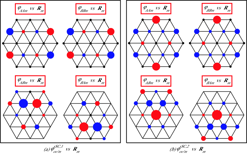
Figure 3: (a) Values of the spin-singlet irreducible singular modes, $\varphi_{oo^{\prime}m}^{{\rm{sSC}},1}$ (a) and $\varphi_{oo^{\prime}m}^{{\rm{sSC}},1}$ (b), for $n_{e}=1.286(\delta=0.286)$. The red and blue circles indicate the positive and negative values, respectively, and the absolute values $\left|{\varphi_{oo^{\prime}m}}\right|$ are encoded by the radius of the circles. The small dots denote the sites ${\bf{R}}_{m}$ having negligible $\varphi_{oo^{\prime}m}$, while the empty sites are eliminated by the filtering process O et al. (2021).

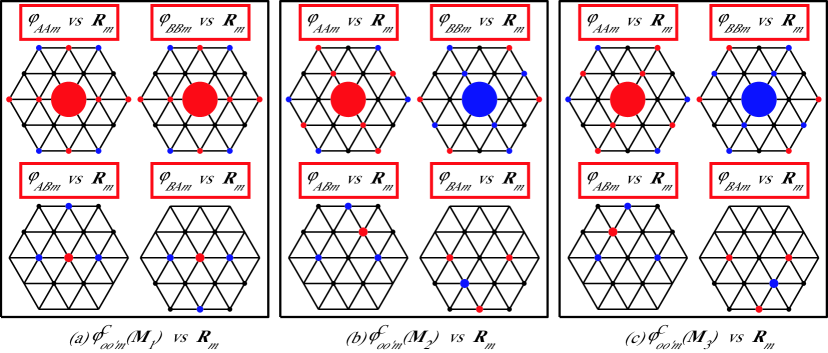
Figure 4: (a) Values of the irreducible singular modes in the spin channel, $\varphi_{oo^{\prime}m}^{\rm{C}}({\bf{M}}_{1})$ (a), $\varphi_{oo^{\prime}m}^{\rm{C}}({\bf{M}}_{2})$ (b), and $\varphi_{oo^{\prime}m}^{\rm{C}}({\bf{M}}_{3})$ (c), for $n_{e}=1.252(\delta=0.252)$. The red and blue circles, the radius of them, the small dots, and the empty sites have the same meanings as in Fig. 3.

As an example, the irreducible singular modes in the pairing channel for $n_{e}=1.286(\delta=0.286)$ and in the spin channel for $n_{e}=1.252(\delta=0.252)$ are shown schematically in Figs. 3 and 4. In Fig. 4, large circles centered at the origin demonstrate that the resulting spin order is a kind of SDW.

In the presence of this SDW, the unit cell gets enlarged, while the BZ reduced. The BZ of the system is shown in Fig. 5(a), compared with the BZ of the honeycomb lattice. Moreover, due to the SC order, a pair of the states associated with momenta ${\bf{k}}$ and $-{\bf{k}}$ are coupled with each other, and therefore, the region of independent momentum becomes half of small BZ (HSBZ). The sampling momentum points in it, employed in the mean-field calculation, are shown in Fig. 5(b).

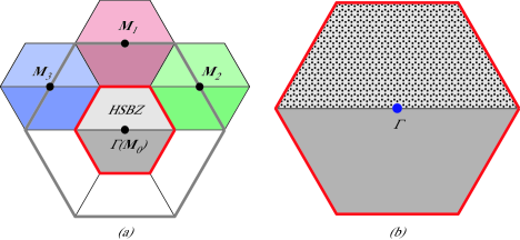
Figure 5: (a) Small BZ reduced by the spin order (small hexagon surrounded by a red border) and the original BZ (large hexagon with a gray border). The spin order couples a momentum in the small BZ with the ones in three little hexagons above it, while the superconducting order links the momenta in a half of the small BZ (HSBZ) to the ones within another half region below it. (b) Sampling points for the momenta in the HSBZ, used in the mean-field calculation. The HSBZ has an area smaller by a factor of eight than that of the original BZ.

One can express the Hamiltonian (91) in terms of ${\bf{\hat{X}}}_{\bf{k}}\equiv({\rm{\hat{C}}}_{\bf{k}},{\rm{\hat{C}}}_{{\bf{k}}+{\bf{M}}_{1}},{\rm{\hat{C}}}_{{\bf{k}}+{\bf{M}}_{2}},{\rm{\hat{C}}}_{{\bf{k}}+{\bf{M}}_{3}},{\rm{\hat{C}}}_{-{\bf{k}}}^{\dagger},{\rm{\hat{C}}}_{-{\bf{k}}+{\bf{M}}_{1}}^{\dagger},{\rm{\hat{C}}}_{-{\bf{k}}+{\bf{M}}_{2}}^{\dagger}$, ${\rm{\hat{C}}}_{-{\bf{k}}+{\bf{M}}_{3}}^{\dagger})^{T}$ with ${\rm{\hat{C}}}_{\bf{k}}\equiv(\hat{c}_{{\bf{k}},A,\uparrow},\hat{c}_{{\bf{k}},A,\downarrow},\hat{c}_{{\bf{k}},B,\uparrow},\hat{c}_{{\bf{k}},B,\downarrow})$. Diagonalizing it, we can obtain 32 eigenstates per momentum in the HSBZ. From the eigenstates for all the sampling points, one can calculate the ground-state energy $E_{G}$ as a function of $\Delta_{1}^{{\rm{sSC}}},\Delta_{2}^{{\rm{sSC}}},\vec{\Delta}^{{\rm{SPN}}}({\bf{M}}_{1}),\vec{\Delta}^{{\rm{SPN}}}({\bf{M}}_{2})$, and $\vec{\Delta}^{{\rm{SPN}}}({\bf{M}}_{3})$. Finally, we can determine the order parameters by minimization of $E_{G}$. In our calculation the resulting order parameters have the form of

$$\begin{split}&\Delta_{1}^{{\rm{sSC}}}=\Delta_{{\rm{sSC}}},\Delta_{2}^{{\rm{sSC}}}=i\Delta_{{\rm{sSC}}},\\ &\vec{\Delta}^{{\rm{SPN}}}({\bf{M}}_{1})=-\Delta_{{\rm{SPN}}}{\bf{e}}_{z},\\ &\vec{\Delta}^{{\rm{SPN}}}({\bf{M}}_{2})=-\Delta_{{\rm{SPN}}}{\bf{e}}_{x},\\ &\vec{\Delta}^{{\rm{SPN}}}({\bf{M}}_{3})=-\Delta_{{\rm{SPN}}}{\bf{e}}_{y},\end{split}$$ (93)

which indicates the chiral SC and SDW orders.

The order parameters $\Delta_{{\rm{sSC}}}$ and $\Delta_{{\rm{SPN}}}$ as a function of the electron density are shown in Fig. 6. For comparison, we calculated the order parameters using our TUFRG+MF scheme, in two ways. In the first calculation we obtained the irreducible bosonic propagators from the TUFRG result of the bosonic propagators at the divergence scale $\Omega_{D}$, and then plugged them into the mean-field calculation. In the second calculation the irreducible bosonic propagators are extracted from the TUFRG result just before entering the divergent regime, namely, from the result at the scale slight larger than $\Omega_{D}$. Comparative analysis of the plots in Fig. 6(a) and Fig. 6(b) demonstrates the robustness of the results of our TUFRG+MF scheme. The plots are characterized by weak and persistent chiral SC order and strong but suddenly disappearing chiral SDW. These features are very similar to the amplitudes of antiferromagnetic and SC gaps in the ground state of the 2D Hubbard model Wang et al. (2014). Near $n_{e}=1.27$, there is an extended region where the chiral SC and chiral SDW orders coexist. In this region the SC order is much smaller than the SDW order. Hence the SC order can be thought as a secondary order within the chiral SDW phase having the unit cell four times larger than the original one. Since the Fermi surface shrinks to two points, the SC order disappears at Van Hove filling. At $n_{e}\approx 1.275$ the SDW order drops suddenly and the plot of $\Delta_{{\rm{sSC}}}$ exhibits a kink, which implies that the two order parameters compete with each other (see the discussion in page 3 of Ref. [Wang et al., 2014]). The drop of the chiral SDW order is related with the generalized Stoner criterion for this instability and the Fermi surface structure away from the nesting.

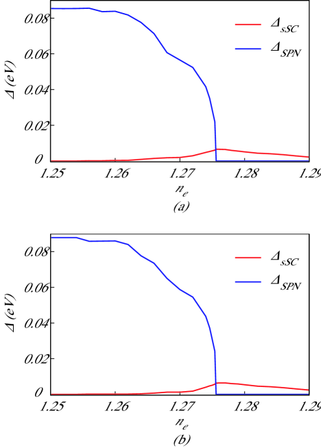
Figure 6: Order parameters $\Delta_{{\rm{sSC}}}$ and $\Delta_{{\rm{SPN}}}$ as a function of $n_{e}$ obtained by the TUFRG+MF calculations starting from the bosonic propagators (a) at the divergence scale $\Omega_{D}$ and (b) just before $\Omega_{D}$, i.e., at $\Omega=\Omega_{D}+\Delta\Omega$. Two plots are nearly identical, demonstrating the robustness of the results of our TUFRG+MF scheme.

V Conclusion

In the present work, we have proposed an approach for combining efficiently the TUFRG and the mean-field theory, extending the efficient FRG+MF scheme Wang et al. (2014) developed by Wang, Eberlein and Metzner. Following the FRG+MF, fluctuation effects from other channels have been neglected in the symmetry-broken regime of the TUFRG flow, yielding the RPA flow of the bosonic propagators. The irreducible bosonic propagators were defined as the initial values of these RPA flow equations. We retained only the dominantly divergent parts of the propagators at the divergence scale, and determined the singular eigenmodes of them. The irreducible bosonic propagators and their eigenmodes (irreducible singular modes) are obtained by resolving inversely the RPA matrix equations. The singular and irreducible singular modes have to satisfy the universal RAS symmetry relations derived from the antisymmetry of Grassmann variables. The mean-field equation based on the irreducible singular modes has been derived by introducing the Hubbard-Stratonovich transformation and employing the saddle-point approximation, in the framework of the path-integral formalism. Details of our TUFRG+MF algorithm are described below:

First, the TUFRG flow equation (44) is integrated until the largest element of some bosonic propagator exceeds a certain value at the divergence scale $\Omega_{D}$. Second, the singular eigenvalues and eigenmodes are found by a diagonalization (Eq. (51)) of the resulting propagators, $P^{\Omega_{D}},C^{\Omega_{D}}$ and $W^{\Omega_{D}}$. Third, the irreducible bosonic propagators (Eqs. (55)–(57)) and the irreducible singular modes (Eqs. (58) and (60)) are determined. The irreducible singular modes in the pairing channel should respect the condition (64) and are divided into the spin-singlet and spin-triplet modes. The modes in the spin and charge channels should satisfy the constraints (66) and (67). Finally, the irreducible coupling constants $\Lambda^{{\rm{X}},\alpha}({\bf{Q}}_{i}^{\rm{X}})$ and singular modes $\left|{\varphi^{{\rm{X}},\alpha}({\bf{Q}}_{i}^{\rm{X}})}\right\rangle$ are inserted into the mean-field equation with the Hamiltonian given by Eq. (86). This equation should be combined with the self-consistency condition (89), leading to final results of the order parameters.

Our novel scheme has been applied to a quantitative analysis of the competing chiral $d$-wave SC and chiral SDW orders, predicted near van Hove filling of the honeycomb lattice. The plot of the magnitudes of both order parameters are obtained as a function of the electron density. Comparative analysis of the plots, which were obtained from the TUFRG results at different scales, indicates the robustness of the results of our TUFRG+MF scheme. The plots are characterized by weak and durable chiral SC order and strong but suddenly dropped chiral SDW, and these features are similar to the previous work where the antiferromagnetic and SC gaps are discussed for the ground state of the 2D Hubbard model. This calculation result shows that our TUFRG+MF approach can elevate the power of the TUFRG to a quantitative level and extend its application to the study of the coexisting orders.

Appendix A Equivalence of critical conditions in RPA and MF theory

We prove the equivalence of two critical conditions in the RPA and the MF theory under the assumption of the positivity of the initial matrices. First, we consider the critical conditions of the RPA. The RPA flow equations in the pairing, spin, and charge channels are, respectively, (See Eq. (50)):

$$\begin{split}&\left[{-P^{\Omega}({\bf{q}})}\right]^{-1}=\left[{-P^{(0)}({\bf{q}})}\right]^{-1}+\chi^{{\rm{pp}}(\Omega)}({\bf{q}}),\\ &\left[{C^{\Omega}({\bf{q}})}\right]^{-1}=\left[{C^{(0)}({\bf{q}})}\right]^{-1}-\chi^{{\rm{ph}}(\Omega)}({\bf{q}}),\left[{W^{\Omega}({\bf{q}})}\right]^{-1}=\left[{W^{(0)}({\bf{q}})}\right]^{-1}-\chi^{{\rm{ph}}(\Omega)}({\bf{q}}).\end{split}$$ (94)

Here $P^{(0)},C^{(0)},$ and $W^{(0)}$ are the initial values of $P^{\Omega},C^{\Omega},$ and $W^{\Omega}$. In our TUFRG+MF they are the irreducible bosonic propagators, $\tilde{P},\tilde{C},$ and $\tilde{W}$, while in the conventional MF theory they would become the initial projection matrices, $V^{{\rm{P}},(0)},V^{{\rm{C}},(0)},$ and $V^{{\rm{W,}}(0)}\equiv V^{{\rm{C,}}(0)}-2V^{{\rm{D,}}(0)}$. They should be Hermitian (Eq. (30)) and satisfy the RAS relations (Eq. (31)):

$$\begin{split}&P_{o^{\prime}_{1}o^{\prime}_{2}m,o_{1}o_{2}n}^{(0)}({\bf{q}})=e^{-i{\bf{R}}_{m}\cdot{\bf{q}}}P_{o^{\prime}_{2}o^{\prime}_{1}\bar{m},o_{2}o_{1}\bar{n}}^{(0)}({\bf{q}})e^{i{\bf{R}}_{n}\cdot{\bf{q}}},\\ &X_{o^{\prime}_{1}o^{\prime}_{2}m,o_{1}o_{2}n}^{(0)}(-{\bf{q}})=e^{i{\bf{R}}_{m}\cdot{\bf{q}}}\left[{X_{o^{\prime}_{2}o^{\prime}_{\rm{1}}\bar{m},o_{\rm{2}}o_{1}\bar{n}}^{(0)}({\bf{q}})}\right]^{*}e^{-i{\bf{R}}_{n}\cdot{\bf{q}}}\textrm{ with }X\in\{C,W\},\hskip 12.0pt\textrm{(RAS)}.\end{split}$$ (95)

For simplicity, we assume that $-P^{(0)},C^{(0)},$ and $W^{(0)}$ are positive matrices like $\tilde{P},\tilde{C},$ and $\tilde{W}$. In this case, the initial matrices, $-P^{(0)},C^{(0)},$ and $W^{(0)}$, can be decomposed in terms of their eigenmodes associated with non-zero positive eigenvalues as done in Eq. (59).

$$\begin{split}\left[{-P^{(0)}({\bf{q}})}\right]=&\sum\limits_{\alpha=1}^{M_{\rm{P}}}{\Lambda^{{\rm{P}},\alpha}({\bf{q}})}\left|{\varphi^{{\rm{P}},\alpha}({\bf{q}})}\right\rangle\left\langle{\varphi^{{\rm{P}},\alpha}({\bf{q}})}\right|,\textrm{ with }\Lambda^{{\rm{P}},\alpha}({\bf{q}})>0,\\ C^{(0)}({\bf{q}})=&\sum\limits_{\alpha=1}^{M_{\rm{C}}}{\Lambda^{{\rm{C}},\alpha}({\bf{q}})}\left|{\varphi^{{\rm{C}},\alpha}({\bf{q}})}\right\rangle\left\langle{\varphi^{{\rm{C}},\alpha}({\bf{q}})}\right|,\textrm{ with }\Lambda^{{\rm{C}},\alpha}({\bf{q}})>0,\\ W^{(0)}({\bf{q}})=&\sum\limits_{\alpha=1}^{M_{\rm{W}}}{\Lambda^{{\rm{W}},\alpha}({\bf{q}})}\left|{\varphi^{{\rm{W}},\alpha}({\bf{q}})}\right\rangle\left\langle{\varphi^{{\rm{W}},\alpha}({\bf{q}})}\right|,\textrm{ with }\Lambda^{{\rm{W}},\alpha}({\bf{q}})>0.\end{split}$$ (96)

Here the eigenmodes have to respect the constraints of Eqs. (64), (66), and (67).

$$\varphi_{oo^{\prime}m}^{{\rm{P}},\alpha}({\bf{q}})=\pm\varphi_{o^{\prime}o\bar{m}}^{{\rm{P}},\alpha}({\bf{q}})e^{-i{\bf{R}}_{m}\cdot{\bf{q}}},$$ (97)

$$\begin{split}\varphi_{oo^{\prime}m}^{{\rm{X}},\alpha}(-{\bf{q}})=[\varphi_{o^{\prime}o\bar{m}}^{{\rm{X}},\alpha}({\bf{q}})]^{*}e^{i{\bf{R}}_{m}\cdot{\bf{q}}}\textrm{ with }{\rm{X}}\in\{{\rm{C}},{\rm{W}}\}.\end{split}$$ (98)

The eigenmodes of $P^{(0)}$ are divided into two sets, i.e., the spin-singlet $\left\{{\left|{\varphi^{{\rm{sSC}},\alpha}}\right\rangle}\right\}$ and the spin-triplet $\left\{{\left|{\varphi^{{\rm{tSC}},\alpha}}\right\rangle}\right\}$ modes, which satisfy

$$\begin{split}\varphi_{oo^{\prime}m}^{{\rm{sSC}},\alpha}({\bf{q}})=+\varphi_{o^{\prime}o\bar{m}}^{{\rm{sSC}},\alpha}({\bf{q}})e^{-i{\bf{R}}_{m}\cdot{\bf{q}}},\varphi_{oo^{\prime}m}^{{\rm{tSC}},\alpha}({\bf{q}})=-\varphi_{o^{\prime}o\bar{m}}^{{\rm{tSC}},\alpha}({\bf{q}})e^{-i{\bf{R}}_{m}\cdot{\bf{q}}}.\end{split}$$ (99)

Due to the positivity of $-P^{(0)},C^{(0)},$ and $W^{(0)}$, we can introduce

$$\begin{split}&\sqrt{-P^{(0)}({\bf{q}})}=\sum\limits_{\alpha=1}^{M_{\rm{P}}}{\sqrt{\Lambda^{{\rm{P}},\alpha}({\bf{q}})}}\left|{\varphi^{{\rm{P}},\alpha}({\bf{q}})}\right\rangle\left\langle{\varphi^{{\rm{P}},\alpha}({\bf{q}})}\right|,\\ &\sqrt{C^{(0)}({\bf{q}})}=\sum\limits_{\alpha=1}^{M_{\rm{C}}}{\sqrt{\Lambda^{{\rm{C}},\alpha}({\bf{q}})}}\left|{\varphi^{{\rm{C}},\alpha}({\bf{q}})}\right\rangle\left\langle{\varphi^{{\rm{C}},\alpha}({\bf{q}})}\right|,\sqrt{W^{(0)}({\bf{q}})}=\sum\limits_{\alpha=1}^{M_{\rm{W}}}{\sqrt{\Lambda^{{\rm{W}},\alpha}({\bf{q}})}}\left|{\varphi^{{\rm{W}},\alpha}({\bf{q}})}\right\rangle\left\langle{\varphi^{{\rm{W}},\alpha}({\bf{q}})}\right|,\end{split}$$ (100)

and rewrite Eq. (94) as follows:

$$\begin{split}-P^{\Omega}({\bf{q}})=&\sqrt{-P^{(0)}({\bf{q}})}\left({1+\sqrt{-P^{(0)}({\bf{q}})}\chi^{{\rm{pp}}(\Omega)}({\bf{q}})\sqrt{-P^{(0)}({\bf{q}})}}\right)^{-1}\sqrt{-P^{(0)}({\bf{q}})},\\ C^{\Omega}({\bf{q}})=&\sqrt{C^{(0)}({\bf{q}})}\left({1-\sqrt{C^{(0)}({\bf{q}})}\chi^{{\rm{ph}}(\Omega)}({\bf{q}})\sqrt{C^{(0)}({\bf{q}})}}\right)^{-1}\sqrt{C^{(0)}({\bf{q}})},\\ W^{\Omega}({\bf{q}})=&\sqrt{W^{(0)}({\bf{q}})}\left({1-\sqrt{W^{(0)}({\bf{q}})}\chi^{{\rm{ph}}(\Omega)}({\bf{q}})\sqrt{W^{(0)}({\bf{q}})}}\right)^{-1}\sqrt{W^{(0)}({\bf{q}})}.\end{split}$$ (101)

Inserting Eq. (100) into Eq. (101) and setting $\Omega$ as $\Omega=0$, we get the final results of the RPA flows.

$$\begin{split}-P^{\Omega=0}({\bf{q}})=&\sum\limits_{\alpha=1}^{M_{\rm{P}}}{\sum\limits_{\beta=1}^{M_{\rm{P}}}{\left[{\sqrt{\Lambda^{\rm{P}}({\bf{q}})}\left({1+\sqrt{\Lambda^{\rm{P}}({\bf{q}})}X^{{\rm{pp}}}({\bf{q}})\sqrt{\Lambda^{\rm{P}}({\bf{q}})}}\right)^{-1}\sqrt{\Lambda^{\rm{P}}({\bf{q}})}}\right]_{\alpha\beta}}}\left|{\varphi^{{\rm{P}},\alpha}({\bf{q}})}\right\rangle\left\langle{\varphi^{{\rm{P}},\beta}({\bf{q}})}\right|,\\ C^{\Omega=0}({\bf{q}})=&\sum\limits_{\alpha=1}^{M_{\rm{C}}}{\sum\limits_{\beta=1}^{M_{\rm{C}}}{\left[{\sqrt{\Lambda^{\rm{C}}({\bf{q}})}\left({1-\sqrt{\Lambda^{\rm{C}}({\bf{q}})}X^{{\rm{ph,C}}}({\bf{q}})\sqrt{\Lambda^{\rm{C}}({\bf{q}})}}\right)^{-1}\sqrt{\Lambda^{\rm{C}}({\bf{q}})}}\right]_{\alpha\beta}}}\left|{\varphi^{{\rm{C}},\alpha}({\bf{q}})}\right\rangle\left\langle{\varphi^{{\rm{C}},\beta}({\bf{q}})}\right|,\\ W^{\Omega=0}({\bf{q}})=&\sum\limits_{\alpha=1}^{M_{\rm{W}}}{\sum\limits_{\beta=1}^{M_{\rm{W}}}{\left[{\sqrt{\Lambda^{\rm{W}}({\bf{q}})}\left({1-\sqrt{\Lambda^{\rm{W}}({\bf{q}})}X^{{\rm{ph,W}}}({\bf{q}})\sqrt{\Lambda^{\rm{W}}({\bf{q}})}}\right)^{-1}\sqrt{\Lambda^{\rm{W}}({\bf{q}})}}\right]_{\alpha\beta}}}\left|{\varphi^{{\rm{W}},\alpha}({\bf{q}})}\right\rangle\left\langle{\varphi^{{\rm{W}},\beta}({\bf{q}})}\right|.\end{split}$$ (102)

Here three diagonal matrices, $\Lambda^{\rm{P}}({\bf{q}}),\Lambda^{\rm{C}}({\bf{q}}),$ and $\Lambda^{\rm{W}}({\bf{q}})$, are given by

$$\begin{split}\Lambda_{\alpha\beta}^{\rm{P}}({\bf{q}})\equiv\Lambda^{{\rm{P}},\alpha}({\bf{q}})\delta_{\alpha\beta},\Lambda_{\alpha\beta}^{\rm{C}}({\bf{q}})\equiv\Lambda^{{\rm{C}},\alpha}({\bf{q}})\delta_{\alpha\beta},\Lambda_{\alpha\beta}^{\rm{W}}({\bf{q}})\equiv\Lambda^{{\rm{W}},\alpha}({\bf{q}})\delta_{\alpha\beta},\end{split}$$ (103)

and three matrices, $X^{{\rm{pp}}}({\bf{q}}),X^{{\rm{ph,C}}}({\bf{q}}),$ and $X^{{\rm{ph,W}}}({\bf{q}})$, are defined by

$$\begin{split}&X_{\alpha\beta}^{{\rm{pp}}}({\bf{q}})\equiv\left\langle{\varphi^{{\rm{P}},\alpha}({\bf{q}})}\right|\chi^{{\rm{pp}}(\Omega=0)}({\bf{q}})\left|{\varphi^{{\rm{P}},\beta}({\bf{q}})}\right\rangle,\\ &X_{\alpha\beta}^{{\rm{ph,C}}}({\bf{q}})\equiv\left\langle{\varphi^{{\rm{C}},\alpha}({\bf{q}})}\right|\chi^{{\rm{ph}}(\Omega=0)}({\bf{q}})\left|{\varphi^{{\rm{C}},\beta}({\bf{q}})}\right\rangle,X_{\alpha\beta}^{{\rm{ph,W}}}({\bf{q}})\equiv\left\langle{\varphi^{{\rm{W}},\alpha}({\bf{q}})}\right|\chi^{{\rm{ph}}(\Omega=0)}({\bf{q}})\left|{\varphi^{{\rm{W}},\beta}({\bf{q}})}\right\rangle.\end{split}$$ (104)

The critical condition of the RPA in the pairing channel is given by the requirement that the matrix $-P^{\Omega=0}({\bf{q}})$ should have an eigenvector associated with infinite eigenvalue. It can be represented by the following equation:

$$\begin{split}\sum\limits_{\beta=1}^{M_{\rm{P}}}{\left[{\sqrt{\Lambda^{\rm{P}}({\bf{q}})}\left({1+\sqrt{\Lambda^{\rm{P}}({\bf{q}})}X^{{\rm{pp}}}({\bf{q}})\sqrt{\Lambda^{\rm{P}}({\bf{q}})}}\right)^{-1}\sqrt{\Lambda^{\rm{P}}({\bf{q}})}}\right]_{\alpha\beta}}C_{\beta}=\mathop{\lim}\limits_{\lambda\to\infty}\lambda C_{\alpha},\end{split}$$

or equivalently,

$$\begin{split}\sum\limits_{\beta=1}^{M_{\rm{P}}}{\left[{\left({\sqrt{\Lambda^{\rm{P}}({\bf{q}})}}\right)^{-1}\left({1+\sqrt{\Lambda^{\rm{P}}({\bf{q}})}X^{{\rm{pp}}}({\bf{q}})\sqrt{\Lambda^{\rm{P}}({\bf{q}})}}\right)\left({\sqrt{\Lambda^{\rm{P}}({\bf{q}})}}\right)^{-1}}\right]_{\alpha\beta}}C_{\beta}=\mathop{\lim}\limits_{\lambda\to\infty}\frac{1}{\lambda}C_{\alpha}=0.\end{split}$$

Due to the finiteness of the diagonal matrix $\sqrt{\Lambda^{\rm{P}}({\bf{q}})}$, this condition is satisfied only if

$$\begin{split}\sum\limits_{\beta=1}^{M_{\rm{P}}}{\left({1+\sqrt{\Lambda^{\rm{P}}({\bf{q}})}X^{{\rm{pp}}}({\bf{q}})\sqrt{\Lambda^{\rm{P}}({\bf{q}})}}\right)_{\alpha\beta}}\left({\frac{{C_{\beta}}}{{\sqrt{\Lambda^{{\rm{P}},\beta}({\bf{q}})}}}}\right)=0.\end{split}$$

This indicates that the matrix $\sqrt{\Lambda^{\rm{P}}({\bf{q}})}X^{{\rm{pp}}}({\bf{q}})\sqrt{\Lambda^{\rm{P}}({\bf{q}})}$ should have the eigenvalue of $-1$. Thus we have the critical condition at ${\bf{q}}={\bf{Q}}_{i}^{\rm{P}}$.

$$\begin{split}&\sum\limits_{\beta=1}^{M_{{\rm{P}},i}}{\left\{{\sqrt{\Lambda^{{\rm{P,}}\alpha}({\bf{Q}}_{i}^{\rm{P}})}}\right.}\left[{-X_{\alpha\beta}^{{\rm{pp}}}({\bf{Q}}_{i}^{\rm{P}})}\right]\left.{\sqrt{\Lambda^{{\rm{P,}}\beta}({\bf{Q}}_{i}^{\rm{P}})}}\right\}Y_{\beta}=Y_{\alpha},\\ &\textrm{(Critical condition of the RPA in the pairing channel)}.\end{split}$$ (105)

In a similar way, we can obtain the critical conditions of the RPA in the spin and charge channels, which read:

$$\begin{split}&\sum\limits_{\beta=1}^{M_{{\rm{C}},i}}{\left\{{\sqrt{\Lambda^{{\rm{C,}}\alpha}({\bf{Q}}_{i}^{\rm{C}})}}\right.}X_{\alpha\beta}^{{\rm{ph,C}}}({\bf{Q}}_{i}^{\rm{C}})\left.{\sqrt{\Lambda^{{\rm{C,}}\beta}({\bf{Q}}_{i}^{\rm{C}})}}\right\}Y_{\beta}=Y_{\alpha},\\ &\textrm{(Critical condition of the RPA in the spin channel)},\end{split}$$ (106)

$$\begin{split}&\sum\limits_{\beta=1}^{M_{{\rm{W}},i}}{\left\{{\sqrt{\Lambda^{{\rm{W,}}\alpha}({\bf{Q}}_{i}^{\rm{W}})}}\right.}X_{\alpha\beta}^{{\rm{ph,W}}}({\bf{Q}}_{i}^{\rm{W}})\left.{\sqrt{\Lambda^{{\rm{W,}}\beta}({\bf{Q}}_{i}^{\rm{W}})}}\right\}Y_{\beta}=Y_{\alpha},\\ &\textrm{(Critical condition of the RPA in the charge channel)}.\end{split}$$ (107)

The critical condition (105) can be expressed more concisely. Starting from the definition of $\chi^{{\rm{pp}}(\Omega)}({\bf{q}})$ (Eq. (25)), one can easily derive following relation:

$$\begin{split}\chi_{o^{\prime}_{1}o^{\prime}_{2}m,o_{1}o_{2}n}^{{\rm{pp}}(\Omega)}({\bf{q}})=e^{-i{\bf{R}}_{m}\cdot{\bf{q}}}\chi_{o^{\prime}_{2}o^{\prime}_{1}\bar{m},o_{2}o_{1}\bar{n}}^{{\rm{pp}}(\Omega)}({\bf{q}})e^{i{\bf{R}}_{n}\cdot{\bf{q}}}.\end{split}$$ (108)

Combining Eqs. (99) and (108), we obtain

$$\begin{split}\left\langle{\varphi^{{\rm{sSC}},\alpha}({\bf{q}})}\right|\chi^{{\rm{pp}}(\Omega)}({\bf{q}})\left|{\varphi^{{\rm{tSC}},\beta}({\bf{q}})}\right\rangle=\left\langle{\varphi^{{\rm{tSC}},\alpha}({\bf{q}})}\right|\chi^{{\rm{pp}}(\Omega)}({\bf{q}})\left|{\varphi^{{\rm{sSC}},\beta}({\bf{q}})}\right\rangle=0,\end{split}$$ (109)

which demonstrates that each of the two sets, $\left\{{\left|{\varphi^{{\rm{sSC}},\alpha}}\right\rangle}\right\}$ and $\left\{{\left|{\varphi^{{\rm{tSC}},\alpha}}\right\rangle}\right\}$, becomes the invariant subspace with respect to the matrix $X^{{\rm{pp}}}({\bf{q}})$. Therefore, the critical condition (105) is divided into two separate conditions for the spin-singlet and spin-triplet pairing channels.

$$\begin{split}&\sum\limits_{\beta=1}^{M_{{\rm{sSC}},i}}{\left\{{\sqrt{\Lambda^{{\rm{sSC,}}\alpha}({\bf{Q}}_{i}^{\rm{P}})}}\right.}\left[{-X_{\alpha\beta}^{{\rm{pp,sSC}}}({\bf{Q}}_{i}^{\rm{P}})}\right]\left.{\sqrt{\Lambda^{{\rm{sSC,}}\beta}({\bf{Q}}_{i}^{\rm{P}})}}\right\}Y_{\beta}=Y_{\alpha},\\ &\textrm{(Critical condition of the RPA in the spin-singlet pairing channel)},\end{split}$$ (110)

$$\begin{split}&\sum\limits_{\beta=1}^{M_{{\rm{tSC}},i}}{\left\{{\sqrt{\Lambda^{{\rm{tSC,}}\alpha}({\bf{Q}}_{i}^{\rm{P}})}}\right.}\left[{-X_{\alpha\beta}^{{\rm{pp,tSC}}}({\bf{Q}}_{i}^{\rm{P}})}\right]\left.{\sqrt{\Lambda^{{\rm{tSC,}}\beta}({\bf{Q}}_{i}^{\rm{P}})}}\right\}Y_{\beta}=Y_{\alpha},\\ &\textrm{(Critical condition of the RPA in the spin-triplet pairing channel)}.\end{split}$$ (111)

Second, we consider the critical conditions of the MF theory. All discussions in Sec. III are valid here, except for the irreducible bosonic propagators, $\tilde{P},\tilde{C},$ and $\tilde{W}$, replaced with $P^{(0)},C^{(0)},$ and $W^{(0)}$. The self-consistency conditions are given by (see Eq. (83))

$$\begin{split}&\Delta_{\alpha}^{{\rm{sSC}}}({\bf{Q}}_{i}^{\rm{P}})=\frac{{\Lambda^{{\rm{sSC}},\alpha}({\bf{Q}}_{i}^{\rm{P}})}}{{4N\beta\hbar}}\left\langle{O_{\alpha}^{{\rm{sSC}}}({\bf{Q}}_{i}^{\rm{P}})}\right\rangle_{\Delta},\vec{\Delta}_{\alpha}^{{\rm{tSC}}}({\bf{Q}}_{i}^{\rm{P}})=\frac{{\Lambda^{{\rm{tSC}},\alpha}({\bf{Q}}_{i}^{\rm{P}})}}{{4N\beta\hbar}}\left\langle{\vec{O}_{\alpha}^{{\rm{tSC}}}({\bf{Q}}_{i}^{\rm{P}})}\right\rangle_{\Delta},\\ &\vec{\Delta}_{\alpha}^{{\rm{SPN}}}({\bf{Q}}_{i}^{\rm{C}})=\frac{{\Lambda^{{\rm{C}},\alpha}({\bf{Q}}_{i}^{\rm{C}})}}{{4N\beta\hbar}}\left\langle{\vec{O}_{\alpha}^{{\rm{SPN}}}({\bf{Q}}_{i}^{\rm{C}})}\right\rangle_{\Delta},\Delta_{\alpha}^{{\rm{CHG}}}({\bf{Q}}_{i}^{\rm{W}})=\frac{{\Lambda^{{\rm{W}},\alpha}({\bf{Q}}_{i}^{\rm{W}})}}{{4N\beta\hbar}}\left\langle{O_{\alpha}^{{\rm{CHG}}}({\bf{Q}}_{i}^{\rm{W}})}\right\rangle_{\Delta}.\end{split}$$ (112)

Here the mean values are defined as

$$\begin{split}\left\langle A\right\rangle_{\Delta}\equiv\frac{{\int{D\bar{\psi}{\kern 1.0pt}D\psi}\exp\{-S_{0}[\psi,\bar{\psi}]-S_{{\rm{HS}}}[\psi,\bar{\psi};\{\Delta^{*}\},\{\Delta\}]\}A}}{{\int{D\bar{\psi}{\kern 1.0pt}D\psi}\exp\{-S_{0}[\psi,\bar{\psi}]-S_{{\rm{HS}}}[\psi,\bar{\psi};\{\Delta^{*}\},\{\Delta\}]\}}},\end{split}$$ (113)

with $S_{0}$ given in Eq. (3), and $S_{{\rm{HS}}}$ defined by Eqs. (74)–(77) and (79). And the fermion bilinears in four channels, $O_{\alpha}^{{\rm{sSC}}}({\bf{q}}),\vec{O}_{\alpha}^{{\rm{tSC}}}({\bf{q}}),\vec{O}_{\alpha}^{{\rm{SPN}}}({\bf{q}}),$ and $O_{\alpha}^{{\rm{CHG}}}({\bf{q}})$ are defined by Eq. (69). In the limit of $\left\{{\Delta^{*}}\right\}\to 0$ and $\left\{\Delta\right\}\to 0$, the additional action $S_{{\rm{HS}}}$ vanishes, and we have

$$\exp\left\{{-S_{{\rm{HS}}}[\psi,\bar{\psi};\{\Delta^{*}\},\{\Delta\}]}\right\}\approx 1-S_{{\rm{HS}}}[\psi,\bar{\psi};\{\Delta^{*}\},\{\Delta\}],$$

from which the following equation is obtained.

$$\begin{split}\left\langle A\right\rangle_{\Delta}\approx\frac{{\left\langle A\right\rangle_{0}-\left\langle{AS_{{\rm{HS}}}[\psi,\bar{\psi};\{\Delta^{*}\},\{\Delta\}]}\right\rangle_{0}}}{{1-\left\langle{S_{{\rm{HS}}}[\psi,\bar{\psi};\{\Delta^{*}\},\{\Delta\}]}\right\rangle_{0}}}=\left\langle A\right\rangle_{0}+\frac{{\left\langle A\right\rangle_{0}\left\langle{S_{{\rm{HS}}}[\psi,\bar{\psi};\{\Delta^{*}\},\{\Delta\}]}\right\rangle_{0}-\left\langle{AS_{{\rm{HS}}}[\psi,\bar{\psi};\{\Delta^{*}\},\{\Delta\}]}\right\rangle_{0}}}{{1-\left\langle{S_{{\rm{HS}}}[\psi,\bar{\psi};\{\Delta^{*}\},\{\Delta\}]}\right\rangle_{0}}}\end{split}$$

Here we introduced a notation $\left\langle A\right\rangle_{0}\equiv\frac{{\int{D\bar{\psi}D\psi}\exp\left({-S_{0}}\right)A}}{{\int{D\bar{\psi}D\psi}\exp\left({-S_{0}}\right)}}$. Since $S_{{\rm{HS}}}$ has the order of magnitude of $\{\Delta^{*}\}$ and $\{\Delta\}$, the above equation becomes

$$\begin{split}\left\langle A\right\rangle_{\Delta}=\left\langle A\right\rangle_{0}+\left\langle A\right\rangle_{0}\left\langle{S_{{\rm{HS}}}[\psi,\bar{\psi};\{\Delta^{*}\},\{\Delta\}]}\right\rangle_{0}-\left\langle{AS_{{\rm{HS}}}[\psi,\bar{\psi};\{\Delta^{*}\},\{\Delta\}]}\right\rangle_{0}+O\left({\left\{{\left|\Delta\right|^{2}}\right\}}\right).\end{split}$$ (114)

Let us consider the mean value $\left\langle{O_{\alpha}^{{\rm{sSC}}}({\bf{Q}}_{i}^{\rm{P}})}\right\rangle_{\Delta}$. Because of $\left\langle{O_{\alpha}^{{\rm{sSC}}}({\bf{Q}}_{i}^{\rm{P}})}\right\rangle_{0}=0$, we have

$$\begin{split}\left\langle{O_{\alpha}^{{\rm{sSC}}}({\bf{Q}}_{i}^{\rm{P}})}\right\rangle_{\Delta}\approx&-\left\langle{O_{\alpha}^{{\rm{sSC}}}({\bf{Q}}_{i}^{\rm{P}})S_{{\rm{HS}}}[\psi,\bar{\psi};\{\Delta^{*}\},\{\Delta\}]}\right\rangle_{0}=-\left\langle{O_{\alpha}^{{\rm{sSC}}}({\bf{Q}}_{i}^{\rm{P}})}\right.\left({S_{{\rm{HS}}}^{{\rm{sSC}}}[\psi,\bar{\psi};\Delta_{{\rm{sSC}}}^{*},\Delta_{{\rm{sSC}}}]}\right.\\ &+S_{{\rm{HS}}}^{{\rm{tSC}}}[\psi,\bar{\psi};\vec{\Delta}_{{\rm{tSC}}}^{*},\vec{\Delta}_{{\rm{tSC}}}]+S_{{\rm{HS}}}^{{\rm{SPN}}}[\psi,\bar{\psi};\vec{\Delta}_{{\rm{SPN}}}^{*},\vec{\Delta}_{{\rm{SPN}}}]+\left.{\left.{S_{{\rm{HS}}}^{{\rm{CHG}}}[\psi,\bar{\psi};\Delta_{{\rm{CHG}}}^{*},\Delta_{{\rm{CHG}}}]}\right)}\right\rangle_{0}.\end{split}$$ (115)

Inserting Eq. (74) into the above equation, one can rewrite the first term in it as follows:

$$\begin{split}&\left\langle{O_{\alpha}^{{\rm{sSC}}}({\bf{Q}}_{i}^{\rm{P}})S_{{\rm{HS}}}^{{\rm{sSC}}}[\psi,\bar{\psi};\Delta_{{\rm{sSC}}}^{*},\Delta_{{\rm{sSC}}}]}\right\rangle_{0}=\\ &\hskip 12.0pt-\frac{1}{\hbar}\sum\limits_{j=1}^{N_{\rm{P}}}{\sum\limits_{\beta=1}^{M_{{\rm{sSC}},j}}{\left\{{\left[{\Delta_{\beta}^{{\rm{sSC}}}({\bf{Q}}_{j}^{\rm{P}})}\right]^{*}}\right.}}\left\langle{O_{\alpha}^{{\rm{sSC}}}({\bf{Q}}_{i}^{\rm{P}})O_{\beta}^{{\rm{sSC}}}({\bf{Q}}_{j}^{\rm{P}})}\right\rangle_{0}+\left.{\Delta_{\beta}^{{\rm{sSC}}}({\bf{Q}}_{j}^{\rm{P}})\left\langle{O_{\alpha}^{{\rm{sSC}}}({\bf{Q}}_{i}^{\rm{P}})\left[{O_{\beta}^{{\rm{sSC}}}({\bf{Q}}_{j}^{\rm{P}})}\right]^{*}}\right\rangle_{0}}\right\}\\ &\hskip 12.0pt=-\frac{1}{\hbar}\sum\limits_{\beta=1}^{M_{{\rm{sSC}},i}}{\Delta_{\beta}^{{\rm{sSC}}}({\bf{Q}}_{i}^{\rm{P}})}\left\langle{O_{\alpha}^{{\rm{sSC}}}({\bf{Q}}_{i}^{\rm{P}})\left[{O_{\beta}^{{\rm{sSC}}}({\bf{Q}}_{i}^{\rm{P}})}\right]^{*}}\right\rangle_{0}.\end{split}$$ (116)

Here we used the relations of

$$\left\langle{O_{\alpha}^{{\rm{sSC}}}({\bf{Q}}_{i}^{\rm{P}})O_{\beta}^{{\rm{sSC}}}({\bf{Q}}_{j}^{\rm{P}})}\right\rangle_{0}=0,\left\langle{O_{\alpha}^{{\rm{sSC}}}({\bf{Q}}_{i}^{\rm{P}})\left[{O_{\beta}^{{\rm{sSC}}}({\bf{Q}}_{j}^{\rm{P}})}\right]^{*}}\right\rangle_{0}=\delta_{ij}\left\langle{O_{\alpha}^{{\rm{sSC}}}({\bf{Q}}_{i}^{\rm{P}})\left[{O_{\beta}^{{\rm{sSC}}}({\bf{Q}}_{i}^{\rm{P}})}\right]^{*}}\right\rangle_{0}.$$

Inserting the first equation in Eq. (69) into Eq. (116), we have

$$\begin{split}&\left\langle{O_{\alpha}^{{\rm{sSC}}}({\bf{Q}}_{i}^{\rm{P}})S_{{\rm{HS}}}^{{\rm{sSC}}}[\psi,\bar{\psi};\Delta_{{\rm{sSC}}}^{*},\Delta_{{\rm{sSC}}}]}\right\rangle_{0}=-\frac{1}{\hbar}\sum\limits_{\beta=1}^{M_{{\rm{sSC}},i}}{\Delta_{\beta}^{{\rm{sSC}}}({\bf{Q}}_{i}^{\rm{P}})}\left\langle{O_{\alpha}^{{\rm{sSC}}}({\bf{Q}}_{i}^{\rm{P}})\left[{O_{\beta}^{{\rm{sSC}}}({\bf{Q}}_{i}^{\rm{P}})}\right]^{*}}\right\rangle_{0}\\ &=-\frac{1}{\hbar}\sum\limits_{\beta=1}^{M_{{\rm{sSC}},i}}{\Delta_{\beta}^{{\rm{sSC}}}({\bf{Q}}_{i}^{\rm{P}})}\sum\limits_{{\bf{p}},\omega_{p}}{\sum\limits_{o,o^{\prime},m}{[\varphi_{oo^{\prime}m}^{{\rm{sSC}},\alpha}({\bf{Q}}_{i}^{\rm{P}})]^{*}e^{i{\bf{R}}_{m}\cdot{\bf{p}}}}}\sum\limits_{{\bf{k}},\omega_{k}}{\sum\limits_{\tilde{o},\tilde{o}^{\prime},n}{\varphi_{\tilde{o}\tilde{o}^{\prime}n}^{{\rm{sSC}},\beta}({\bf{Q}}_{i}^{\rm{P}})e^{-i{\bf{R}}_{n}\cdot{\bf{k}}}}}\\ &\hskip 12.0pt\times\sum\limits_{\sigma,\sigma^{\prime}}{\sigma\sigma^{\prime}}\left\langle{\psi_{-\sigma}(-{\bf{p}},-\omega_{p},o^{\prime})\psi_{\sigma}({\bf{p}}+{\bf{Q}}_{i}^{\rm{P}},\omega_{p},o)\bar{\psi}_{\sigma^{\prime}}({\bf{k}}+{\bf{Q}}_{i}^{\rm{P}},\omega_{k},\tilde{o})\bar{\psi}_{-\sigma^{\prime}}(-{\bf{k}},-\omega_{k},\tilde{o}^{\prime})}\right\rangle_{0}.\end{split}$$ (117)

We can use Wick’s theorem Negele and Orland (1988) to evaluate the mean value in the above equation.

$$\begin{split}&\sum\limits_{\sigma,\sigma^{\prime}}{\sigma\sigma^{\prime}}\left\langle{\psi_{-\sigma}(-{\bf{p}},-\omega_{p},o^{\prime})\psi_{\sigma}({\bf{p}}+{\bf{Q}}_{i}^{\rm{P}},\omega_{p},o)\bar{\psi}_{\sigma^{\prime}}({\bf{k}}+{\bf{Q}}_{i}^{\rm{P}},\omega_{k},\tilde{o})\bar{\psi}_{-\sigma^{\prime}}(-{\bf{k}},-\omega_{k},\tilde{o}^{\prime})}\right\rangle_{0}\\ &=\sum\limits_{\sigma,\sigma^{\prime}}{\sigma\sigma^{\prime}}\left\langle{\psi_{-\sigma}(-{\bf{p}},-\omega_{p},o^{\prime})\bar{\psi}_{-\sigma^{\prime}}(-{\bf{k}},-\omega_{k},\tilde{o}^{\prime})}\right\rangle_{0}\left\langle{\psi_{\sigma}({\bf{p}}+{\bf{Q}}_{i}^{\rm{P}},\omega_{p},o)\bar{\psi}_{\sigma^{\prime}}({\bf{k}}+{\bf{Q}}_{i}^{\rm{P}},\omega_{k},\tilde{o})}\right\rangle_{0}\\ &+\sum\limits_{\sigma,\sigma^{\prime}}{\sigma\sigma^{\prime}}(-1)\left\langle{\psi_{-\sigma}(-{\bf{p}},-\omega_{p},o^{\prime})\bar{\psi}_{\sigma^{\prime}}({\bf{k}}+{\bf{Q}}_{i}^{\rm{P}},\omega_{k},\tilde{o})}\right\rangle_{0}\left\langle{\psi_{\sigma}({\bf{p}}+{\bf{Q}}_{i}^{\rm{P}},\omega_{p},o)\bar{\psi}_{-\sigma^{\prime}}(-{\bf{k}},-\omega_{k},\tilde{o}^{\prime})}\right\rangle_{0}\\ &=2\delta_{{\bf{p}},{\bf{k}}}\delta_{\omega_{p},\omega_{k}}G_{o^{\prime}\tilde{o}^{\prime}}^{0}(-{\bf{p}},-\omega_{p})G_{o\tilde{o}}^{0}({\bf{p}}+{\bf{Q}}_{i}^{\rm{P}},\omega_{p})+2\delta_{{\bf{p}},-{\bf{k}}-{\bf{Q}}_{i}^{\rm{P}}}\delta_{\omega_{p},-\omega_{k}}G_{o^{\prime}\tilde{o}}^{0}(-{\bf{p}},-\omega_{p})G_{o\tilde{o}^{\prime}}^{0}({\bf{p}}+{\bf{Q}}_{i}^{\rm{P}},\omega_{p})\end{split}$$

Inserting this result into Eq. (117), we obtain

$$\begin{split}&\left\langle{O_{\alpha}^{{\rm{sSC}}}({\bf{Q}}_{i}^{\rm{P}})S_{{\rm{HS}}}^{{\rm{sSC}}}[\psi,\bar{\psi};\Delta_{{\rm{sSC}}}^{*},\Delta_{{\rm{sSC}}}]}\right\rangle_{0}=-\frac{1}{\hbar}\sum\limits_{\beta=1}^{M_{{\rm{sSC}},i}}{\Delta_{\beta}^{{\rm{sSC}}}({\bf{Q}}_{i}^{\rm{P}})}\sum\limits_{o,o^{\prime},m}{[\varphi_{oo^{\prime}m}^{{\rm{sSC}},\alpha}({\bf{Q}}_{i}^{\rm{P}})]^{*}}\sum\limits_{\tilde{o},\tilde{o}^{\prime},n}{\varphi_{\tilde{o}\tilde{o}^{\prime}n}^{{\rm{sSC}},\beta}({\bf{Q}}_{i}^{\rm{P}})}\\ &\times 2\sum\limits_{{\bf{p}},\omega_{p}}{e^{i{\bf{R}}_{m}\cdot{\bf{p}}}}\left[{e^{-i{\bf{R}}_{n}\cdot{\bf{p}}}}\right.G_{o^{\prime}\tilde{o}^{\prime}}^{0}(-{\bf{p}},-\omega_{p})G_{o\tilde{o}}^{0}({\bf{p}}+{\bf{Q}}_{i}^{\rm{P}},\omega_{p})+\left.{e^{-i{\bf{R}}_{n}\cdot(-{\bf{p}}-{\bf{Q}}_{i}^{\rm{P}})}G_{o^{\prime}\tilde{o}}^{0}(-{\bf{p}},-\omega_{p})G_{o\tilde{o}^{\prime}}^{0}({\bf{p}}+{\bf{Q}}_{i}^{\rm{P}},\omega_{p})}\right]\\ &=-\frac{2}{\hbar}\sum\limits_{\beta=1}^{M_{{\rm{sSC}},i}}{\Delta_{\beta}^{{\rm{sSC}}}({\bf{Q}}_{i}^{\rm{P}})}\sum\limits_{o,o^{\prime},m}{[\varphi_{oo^{\prime}m}^{{\rm{sSC}},\alpha}({\bf{Q}}_{i}^{\rm{P}})]^{*}}\sum\limits_{{\bf{p}},\omega_{p}}{e^{i{\bf{R}}_{m}\cdot{\bf{p}}}}\\ &\times\sum\limits_{\tilde{o},\tilde{o}^{\prime},n}{\left({\varphi_{\tilde{o}\tilde{o}^{\prime}n}^{{\rm{sSC}},\beta}({\bf{Q}}_{i}^{\rm{P}})+\varphi_{\tilde{o}^{\prime}\tilde{o}\bar{n}}^{{\rm{sSC}},\beta}({\bf{Q}}_{i}^{\rm{P}})e^{-i{\bf{R}}_{n}\cdot{\bf{Q}}_{i}^{\rm{P}}}}\right)}e^{-i{\bf{R}}_{n}\cdot{\bf{p}}}G_{o^{\prime}\tilde{o}^{\prime}}^{0}(-{\bf{p}},-\omega_{p})G_{o\tilde{o}}^{0}({\bf{p}}+{\bf{Q}}_{i}^{\rm{P}},\omega_{p}).\end{split}$$

Due to the relation (99), the above equation becomes

$$\begin{split}&\left\langle{O_{\alpha}^{{\rm{sSC}}}({\bf{Q}}_{i}^{\rm{P}})S_{{\rm{HS}}}^{{\rm{sSC}}}[\psi,\bar{\psi};\Delta_{{\rm{sSC}}}^{*},\Delta_{{\rm{sSC}}}]}\right\rangle_{0}=-\frac{4}{\hbar}\sum\limits_{\beta=1}^{M_{{\rm{sSC}},i}}{\Delta_{\beta}^{{\rm{sSC}}}({\bf{Q}}_{i}^{\rm{P}})}\sum\limits_{o,o^{\prime},m}{[\varphi_{oo^{\prime}m}^{{\rm{sSC}},\alpha}({\bf{Q}}_{i}^{\rm{P}})]^{*}}\sum\limits_{\tilde{o},\tilde{o}^{\prime},n}{\varphi_{\tilde{o}\tilde{o}^{\prime}n}^{{\rm{sSC}},\beta}({\bf{Q}}_{i}^{\rm{P}})}\\ &\times\sum\limits_{\bf{p}}{e^{i{\bf{R}}_{m}\cdot{\bf{p}}}}e^{-i{\bf{R}}_{n}\cdot{\bf{p}}}\sum\limits_{\omega_{p}}{G_{o\tilde{o}}^{0}({\bf{p}}+{\bf{Q}}_{i}^{\rm{P}},\omega_{p})G_{o^{\prime}\tilde{o}^{\prime}}^{0}(-{\bf{p}},-\omega_{p})}\\ &=4N\beta\hbar\sum\limits_{\gamma=1}^{M_{{\rm{sSC}},i}}{\Delta_{\gamma}^{{\rm{sSC}}}({\bf{Q}}_{i}^{\rm{P}})}\sum\limits_{o,o^{\prime},m}{[\varphi_{oo^{\prime}m}^{{\rm{sSC}},\alpha}({\bf{Q}}_{i}^{\rm{P}})]^{*}}\sum\limits_{\tilde{o},\tilde{o}^{\prime},n}{\varphi_{\tilde{o}\tilde{o}^{\prime}n}^{{\rm{sSC}},\gamma}({\bf{Q}}_{i}^{\rm{P}})}\chi_{oo^{\prime}m,\tilde{o}\tilde{o}^{\prime}n}^{{\rm{pp(}}\Omega=0{\rm{)}}}({\bf{Q}}_{i}^{\rm{P}}).\end{split}$$

Taking into account the definition (104), we have the final result.

$$\begin{split}\left\langle{O_{\alpha}^{{\rm{sSC}}}({\bf{Q}}_{i}^{\rm{P}})S_{{\rm{HS}}}^{{\rm{sSC}}}[\psi,\bar{\psi};\Delta_{{\rm{sSC}}}^{*},\Delta_{{\rm{sSC}}}]}\right\rangle_{0}=4N\beta\hbar\sum\limits_{\gamma=1}^{M_{{\rm{sSC}},i}}{X_{\alpha\gamma}^{{\rm{pp,sSC}}}({\bf{Q}}_{i}^{\rm{P}})\Delta_{\gamma}^{{\rm{sSC}}}({\bf{Q}}_{i}^{\rm{P}})}\end{split}$$ (118)

In a similar way, one can verify the following relations:

$$\begin{split}&\left\langle{O_{\alpha}^{{\rm{sSC}}}({\bf{Q}}_{i}^{\rm{P}})S_{{\rm{HS}}}^{{\rm{tSC}}}[\psi,\bar{\psi};\vec{\Delta}_{{\rm{tSC}}}^{*},\vec{\Delta}_{{\rm{tSC}}}]}\right\rangle_{0}=\left\langle{O_{\alpha}^{{\rm{sSC}}}({\bf{Q}}_{i}^{\rm{P}})S_{{\rm{HS}}}^{{\rm{SPN}}}[\psi,\bar{\psi};\vec{\Delta}_{{\rm{SPN}}}^{*},\vec{\Delta}_{{\rm{SPN}}}]}\right\rangle_{0}\\ &=\left\langle{O_{\alpha}^{{\rm{sSC}}}({\bf{Q}}_{i}^{\rm{P}})S_{{\rm{HS}}}^{{\rm{CHG}}}[\psi,\bar{\psi};\Delta_{{\rm{CHG}}}^{*},\Delta_{{\rm{CHG}}}]}\right\rangle_{0}=0.\end{split}$$ (119)

Inserting Eqs. (118) and (119) into Eq. (115), we get

$$\begin{split}\left\langle{O_{\alpha}^{{\rm{sSC}}}({\bf{Q}}_{i}^{\rm{P}})}\right\rangle_{\Delta}=-4N\beta\hbar\sum\limits_{\gamma=1}^{M_{{\rm{sSC}},i}}{X_{\alpha\gamma}^{{\rm{pp,sSC}}}({\bf{Q}}_{i}^{\rm{P}})\Delta_{\gamma}^{{\rm{sSC}}}({\bf{Q}}_{i}^{\rm{P}})}.\end{split}$$ (120)

Finally, the first equation in Eq. (112) becomes

$$\begin{split}\Delta_{\alpha}^{{\rm{sSC}}}({\bf{Q}}_{i}^{\rm{P}})=-\Lambda^{{\rm{sSC}},\alpha}({\bf{Q}}_{i}^{\rm{P}})\sum\limits_{\beta=1}^{M_{{\rm{sSC}},i}}{X_{\alpha\beta}^{{\rm{pp,sSC}}}({\bf{Q}}_{i}^{\rm{P}})\Delta_{\beta}^{{\rm{sSC}}}({\bf{Q}}_{i}^{\rm{P}})},\end{split}$$ (121)

or equivalently, with $Y_{\alpha}\equiv\frac{{\Delta_{\alpha}^{{\rm{sSC}}}({\bf{Q}}_{i}^{\rm{P}})}}{{\sqrt{\Lambda^{{\rm{sSC}},\alpha}({\bf{Q}}_{i}^{\rm{P}})}}}$,

$$\begin{split}&\sum\limits_{\beta=1}^{M_{{\rm{sSC}},i}}{\left\{{\sqrt{\Lambda^{{\rm{sSC}},\alpha}({\bf{Q}}_{i}^{\rm{P}})}\left[{-X_{\alpha\beta}^{{\rm{pp,sSC}}}({\bf{Q}}_{i}^{\rm{P}})}\right]\sqrt{\Lambda^{{\rm{sSC}},\beta}({\bf{Q}}_{i}^{\rm{P}})}}\right\}}Y_{\beta}=Y_{\alpha},\\ &\textrm{(Critical condition of the MF theory in the spin-singlet pairing channel)}.\end{split}$$ (122)

This is exactly the same as the critical condition (110).

We consider the mean value $\left\langle{\vec{O}_{\alpha}^{{\rm{tSC}}}({\bf{Q}}_{i}^{\rm{P}})}\right\rangle_{\Delta}$. It is clear that $\left\langle{\vec{O}_{\alpha}^{{\rm{tSC}}}({\bf{Q}}_{i}^{\rm{P}})}\right\rangle_{0}=0$. So we have

$$\begin{split}\left\langle{\vec{O}_{\alpha}^{{\rm{tSC}}}({\bf{Q}}_{i}^{\rm{P}})}\right\rangle_{\Delta}=-\left\langle{\vec{O}_{\alpha}^{{\rm{tSC}}}({\bf{Q}}_{i}^{\rm{P}})}\right.&\left({S_{{\rm{HS}}}^{{\rm{sSC}}}[\psi,\bar{\psi};\Delta_{{\rm{sSC}}}^{*},\Delta_{{\rm{sSC}}}]}\right.+S_{{\rm{HS}}}^{{\rm{tSC}}}[\psi,\bar{\psi};\vec{\Delta}_{{\rm{tSC}}}^{*},\vec{\Delta}_{{\rm{tSC}}}]\\ &+S_{{\rm{HS}}}^{{\rm{SPN}}}[\psi,\bar{\psi};\vec{\Delta}_{{\rm{SPN}}}^{*},\vec{\Delta}_{{\rm{SPN}}}]+\left.{\left.{S_{{\rm{HS}}}^{{\rm{CHG}}}[\psi,\bar{\psi};\Delta_{{\rm{CHG}}}^{*},\Delta_{{\rm{CHG}}}]}\right)}\right\rangle_{0}.\end{split}$$ (123)

Through the procedure similar to the one described above, we obtain the following results:

$$\begin{split}\left\langle{\vec{O}_{\alpha}^{{\rm{tSC}}}({\bf{Q}}_{i}^{\rm{P}})S_{{\rm{HS}}}^{{\rm{tSC}}}[\psi,\bar{\psi};\vec{\Delta}_{{\rm{tSC}}}^{*},\vec{\Delta}_{{\rm{tSC}}}]}\right\rangle_{0}=4N\beta\hbar\sum\limits_{\gamma=1}^{M_{{\rm{tSC}},i}}{X_{\alpha\gamma}^{{\rm{pp,tSC}}}({\bf{Q}}_{i}^{\rm{P}})\vec{\Delta}_{\gamma}^{{\rm{tSC}}}({\bf{Q}}_{i}^{\rm{P}})},\end{split}$$ (124)

$$\begin{split}&\left\langle{\vec{O}_{\alpha}^{{\rm{tSC}}}({\bf{Q}}_{i}^{\rm{P}})S_{{\rm{HS}}}^{{\rm{sSC}}}[\psi,\bar{\psi};\Delta_{{\rm{sSC}}}^{*},\Delta_{{\rm{sSC}}}]}\right\rangle_{0}=\left\langle{\vec{O}_{\alpha}^{{\rm{tSC}}}({\bf{Q}}_{i}^{\rm{P}})S_{{\rm{HS}}}^{{\rm{SPN}}}[\psi,\bar{\psi};\vec{\Delta}_{{\rm{SPN}}}^{*},\vec{\Delta}_{{\rm{SPN}}}]}\right\rangle_{0}\\ &=\left\langle{\vec{O}_{\alpha}^{{\rm{tSC}}}({\bf{Q}}_{i}^{\rm{P}})S_{{\rm{HS}}}^{{\rm{CHG}}}[\psi,\bar{\psi};\Delta_{{\rm{CHG}}}^{*},\Delta_{{\rm{CHG}}}]}\right\rangle_{0}=0.\end{split}$$ (125)

Inserting Eqs. (124) and (125) into Eq. (123), we get

$$\begin{split}\left\langle{\vec{O}_{\alpha}^{{\rm{tSC}}}({\bf{Q}}_{i}^{\rm{P}})}\right\rangle_{\Delta}=-4N\beta\hbar\sum\limits_{\gamma=1}^{M_{{\rm{tSC}},i}}{X_{\alpha\gamma}^{{\rm{pp,tSC}}}({\bf{Q}}_{i}^{\rm{P}})\vec{\Delta}_{\gamma}^{{\rm{tSC}}}({\bf{Q}}_{i}^{\rm{P}})}.\end{split}$$ (126)

Then, the second equation in Eq. (112) becomes

$$\begin{split}\vec{\Delta}_{\alpha}^{{\rm{tSC}}}({\bf{Q}}_{i}^{\rm{P}})=-\Lambda^{{\rm{tSC}},\alpha}({\bf{Q}}_{i}^{\rm{P}})\sum\limits_{\beta=1}^{M_{{\rm{tSC}},i}}{X_{\alpha\beta}^{{\rm{pp,tSC}}}({\bf{Q}}_{i}^{\rm{P}})\vec{\Delta}_{\beta}^{{\rm{tSC}}}({\bf{Q}}_{i}^{\rm{P}})},\end{split}$$ (127)

or equivalently, with $\vec{Y}_{\alpha}\equiv\frac{{\vec{\Delta}_{\alpha}^{{\rm{tSC}}}({\bf{Q}}_{i}^{\rm{P}})}}{{\sqrt{\Lambda^{{\rm{tSC}},\alpha}({\bf{Q}}_{i}^{\rm{P}})}}}$,

$$\begin{split}&\sum\limits_{\beta=1}^{M_{{\rm{tSC}},i}}{\left\{{\sqrt{\Lambda^{{\rm{tSC}},\alpha}({\bf{Q}}_{i}^{\rm{P}})}\left[{-X_{\alpha\beta}^{{\rm{pp,tSC}}}({\bf{Q}}_{i}^{\rm{P}})}\right]\sqrt{\Lambda^{{\rm{tSC}},\beta}({\bf{Q}}_{i}^{\rm{P}})}}\right\}}\vec{Y}_{\beta}=\vec{Y}_{\alpha},\\ &\textrm{(Critical condition of the MF theory in the spin-triplet pairing channel)}.\end{split}$$ (128)

This is exactly the same as the critical condition (111).

Now let us consider the mean value $\left\langle{\vec{O}_{\alpha}^{{\rm{SPN}}}({\bf{Q}}_{i}^{\rm{C}})}\right\rangle_{\Delta}$. Evidently, $\left\langle{\vec{O}_{\alpha}^{{\rm{SPN}}}({\bf{Q}}_{i}^{\rm{C}})}\right\rangle_{0}=0$, and we get

$$\begin{split}\left\langle{\vec{O}_{\alpha}^{{\rm{SPN}}}({\bf{Q}}_{i}^{\rm{C}})}\right\rangle_{\Delta}=-\left\langle{\vec{O}_{\alpha}^{{\rm{SPN}}}({\bf{Q}}_{i}^{\rm{C}})}\right.&\left({S_{{\rm{HS}}}^{{\rm{sSC}}}[\psi,\bar{\psi};\Delta_{{\rm{sSC}}}^{*},\Delta_{{\rm{sSC}}}]}\right.+S_{{\rm{HS}}}^{{\rm{tSC}}}[\psi,\bar{\psi};\vec{\Delta}_{{\rm{tSC}}}^{*},\vec{\Delta}_{{\rm{tSC}}}]\\ &+S_{{\rm{HS}}}^{{\rm{SPN}}}[\psi,\bar{\psi};\vec{\Delta}_{{\rm{SPN}}}^{*},\vec{\Delta}_{{\rm{SPN}}}]+\left.{\left.{S_{{\rm{HS}}}^{{\rm{CHG}}}[\psi,\bar{\psi};\Delta_{{\rm{CHG}}}^{*},\Delta_{{\rm{CHG}}}]}\right)}\right\rangle_{0}.\end{split}$$ (129)

Inserting Eq. (76) into the above equation, one can rewrite the third term in it as follows:

$$\begin{split}&\left\langle{\vec{O}_{\alpha}^{{\rm{SPN}}}({\bf{Q}}_{i}^{\rm{C}})S_{{\rm{HS}}}^{{\rm{SPN}}}[\psi,\bar{\psi};\vec{\Delta}_{{\rm{SPN}}}^{*},\vec{\Delta}_{{\rm{SPN}}}]}\right\rangle_{0}=\\ &\hskip 24.0pt-\frac{1}{\hbar}\sum\limits_{j=1}^{N_{\rm{C}}}{\sum\limits_{\beta=1}^{M_{{\rm{C}},j}}{\left\langle{\vec{O}_{\alpha}^{{\rm{SPN}}}({\bf{Q}}_{i}^{\rm{C}})\left\{{\left[{\vec{\Delta}_{\beta}^{{\rm{SPN}}}({\bf{Q}}_{j}^{\rm{C}})}\right]^{*}\cdot\vec{O}_{\beta}^{{\rm{SPN}}}({\bf{Q}}_{j}^{\rm{C}})}\right.}\right.}}+\left.{\left.{\vec{\Delta}_{\beta}^{{\rm{SPN}}}({\bf{Q}}_{j}^{\rm{C}})\cdot\left[{\vec{O}_{\beta}^{{\rm{SPN}}}({\bf{Q}}_{j}^{\rm{C}})}\right]^{*}}\right\}}\right\rangle_{0}.\end{split}$$

Concretely, its $x$-component reads

$$\begin{split}&\left\langle{O_{\alpha,x}^{{\rm{SPN}}}({\bf{Q}}_{i}^{\rm{C}})S_{{\rm{HS}}}^{{\rm{SPN}}}[\psi,\bar{\psi};\vec{\Delta}_{{\rm{SPN}}}^{*},\vec{\Delta}_{{\rm{SPN}}}]}\right\rangle_{0}=\\ &-\frac{1}{\hbar}\sum\limits_{j=1}^{N_{\rm{C}}}{\sum\limits_{\beta=1}^{M_{{\rm{C}},j}}{\left\langle{O_{\alpha,x}^{{\rm{SPN}}}({\bf{Q}}_{i}^{\rm{C}})\left\{{\left[{\vec{\Delta}_{\beta}^{{\rm{SPN}}}({\bf{Q}}_{j}^{\rm{C}})}\right]^{*}\cdot\vec{O}_{\beta}^{{\rm{SPN}}}({\bf{Q}}_{j}^{\rm{C}})}\right.}\right.}}+\left.{\left.{\vec{\Delta}_{\beta}^{{\rm{SPN}}}({\bf{Q}}_{j}^{\rm{C}})\cdot\left[{\vec{O}_{\beta}^{{\rm{SPN}}}({\bf{Q}}_{j}^{\rm{C}})}\right]^{*}}\right\}}\right\rangle_{0}\\ &=-\frac{1}{\hbar}\sum\limits_{j=1}^{N_{\rm{C}}}{\sum\limits_{\beta=1}^{M_{{\rm{C}},j}}{\left\{{\left[{\vec{\Delta}_{\beta}^{{\rm{SPN}}}({\bf{Q}}_{j}^{\rm{C}})}\right]^{*}\cdot}\right.}}\left\langle{O_{\alpha,x}^{{\rm{SPN}}}({\bf{Q}}_{i}^{\rm{C}})\vec{O}_{\beta}^{{\rm{SPN}}}({\bf{Q}}_{j}^{\rm{C}})}\right\rangle_{0}+\left.{\vec{\Delta}_{\beta}^{{\rm{SPN}}}({\bf{Q}}_{j}^{\rm{C}})\cdot\left\langle{O_{\alpha,x}^{{\rm{SPN}}}({\bf{Q}}_{i}^{\rm{C}})\left[{\vec{O}_{\beta}^{{\rm{SPN}}}({\bf{Q}}_{j}^{\rm{C}})}\right]^{*}}\right\rangle_{0}}\right\}\\ &=-\frac{1}{\hbar}\sum\limits_{\beta=1}^{M_{{\rm{C}},i}}{\left\{{\left[{\vec{\Delta}_{\beta}^{{\rm{SPN}}}(-{\bf{Q}}_{i}^{\rm{C}})}\right]^{*}}\right.}\cdot\left\langle{O_{\alpha,x}^{{\rm{SPN}}}({\bf{Q}}_{i}^{\rm{C}})\vec{O}_{\beta}^{{\rm{SPN}}}(-{\bf{Q}}_{i}^{\rm{C}})}\right\rangle_{0}+\vec{\Delta}_{\beta}^{{\rm{SPN}}}({\bf{Q}}_{i}^{\rm{C}})\cdot\left.{\left\langle{O_{\alpha,x}^{{\rm{SPN}}}({\bf{Q}}_{i}^{\rm{C}})\left[{\vec{O}_{\beta}^{{\rm{SPN}}}({\bf{Q}}_{i}^{\rm{C}})}\right]^{*}}\right\rangle_{0}}\right\}.\end{split}$$

By using the relations,

$$\begin{split}&\left\langle{O_{\alpha,x}^{{\rm{SPN}}}({\bf{Q}}_{i}^{\rm{C}})\vec{O}_{\beta}^{{\rm{SPN}}}({\bf{Q}}_{j}^{\rm{C}})}\right\rangle_{0}=\delta_{{\bf{Q}}_{i}^{\rm{C}},-{\bf{Q}}_{j}^{\rm{C}}}\left\langle{O_{\alpha,x}^{{\rm{SPN}}}({\bf{Q}}_{i}^{\rm{C}})\vec{O}_{\beta}^{{\rm{SPN}}}(-{\bf{Q}}_{i}^{\rm{C}})}\right\rangle_{0},\\ &\left\langle{O_{\alpha,x}^{{\rm{SPN}}}({\bf{Q}}_{i}^{\rm{C}})\left[{\vec{O}_{\beta}^{{\rm{SPN}}}({\bf{Q}}_{j}^{\rm{C}})}\right]^{*}}\right\rangle_{0}=\delta_{ij}\left\langle{O_{\alpha,x}^{{\rm{SPN}}}({\bf{Q}}_{i}^{\rm{C}})\left[{\vec{O}_{\beta}^{{\rm{SPN}}}({\bf{Q}}_{i}^{\rm{C}})}\right]^{*}}\right\rangle_{0},\\ &\left[{\vec{\Delta}_{\beta}^{{\rm{SPN}}}(-{\bf{Q}}_{i}^{\rm{C}})}\right]^{*}=\vec{\Delta}_{\beta}^{{\rm{SPN}}}({\bf{Q}}_{i}^{\rm{C}}),\vec{O}_{\beta}^{{\rm{SPN}}}(-{\bf{Q}}_{i}^{\rm{C}})=\left[{\vec{O}_{\beta}^{{\rm{SPN}}}({\bf{Q}}_{i}^{\rm{C}})}\right]^{*},\end{split}$$

we obtain

$$\begin{split}\left\langle{O_{\alpha,x}^{{\rm{SPN}}}({\bf{Q}}_{i}^{\rm{C}})S_{{\rm{HS}}}^{{\rm{SPN}}}[\psi,\bar{\psi};\vec{\Delta}_{{\rm{SPN}}}^{*},\vec{\Delta}_{{\rm{SPN}}}]}\right\rangle_{0}=-\frac{2}{\hbar}\sum\limits_{\beta=1}^{M_{{\rm{C}},i}}{\vec{\Delta}_{\beta}^{{\rm{SPN}}}({\bf{Q}}_{i}^{\rm{C}})}\cdot\left\langle{O_{\alpha,x}^{{\rm{SPN}}}({\bf{Q}}_{i}^{\rm{C}})\left[{\vec{O}_{\beta}^{{\rm{SPN}}}({\bf{Q}}_{i}^{\rm{C}})}\right]^{*}}\right\rangle_{0}.\end{split}$$ (130)

Inserting the third equation in Eq. (69) into Eq. (130), we have

$$\begin{split}&\left\langle{O_{\alpha,x}^{{\rm{SPN}}}({\bf{Q}}_{i}^{\rm{C}})S_{{\rm{HS}}}^{{\rm{SPN}}}[\psi,\bar{\psi};\vec{\Delta}_{{\rm{SPN}}}^{*},\vec{\Delta}_{{\rm{SPN}}}]}\right\rangle_{0}=-\frac{2}{\hbar}\sum\limits_{\beta=1}^{M_{{\rm{C}},i}}{\vec{\Delta}_{\beta}^{{\rm{SPN}}}({\bf{Q}}_{i}^{\rm{C}})}\cdot\left\langle{O_{\alpha,x}^{{\rm{SPN}}}({\bf{Q}}_{i}^{\rm{C}})\left[{\vec{O}_{\beta}^{{\rm{SPN}}}({\bf{Q}}_{i}^{\rm{C}})}\right]^{*}}\right\rangle_{0}\\ &=-\frac{2}{\hbar}\sum\limits_{\beta=1}^{M_{{\rm{C}},i}}{\sum\limits_{\gamma=x,y,z}{\Delta_{\beta,\gamma}^{{\rm{SPN}}}({\bf{Q}}_{i}^{\rm{C}})}}\sum\limits_{{\bf{p}},\omega_{p}}{\sum\limits_{o,o^{\prime},m}{[\varphi_{oo^{\prime}m}^{{\rm{C}},\alpha}({\bf{Q}}_{i}^{\rm{C}})]^{*}e^{i{\bf{R}}_{m}\cdot{\bf{p}}}}}\sum\limits_{{\bf{k}},\omega_{k}}{\sum\limits_{\tilde{o},\tilde{o}^{\prime},n}{\varphi_{\tilde{o}\tilde{o}^{\prime}n}^{{\rm{C}},\beta}({\bf{Q}}_{i}^{\rm{C}})e^{-i{\bf{R}}_{n}\cdot{\bf{k}}}}}\\ &\times\sum\limits_{\sigma,\sigma^{\prime}}{\sigma_{\sigma\sigma^{\prime}}^{x}\sum\limits_{s,s^{\prime}}{\left[{\sigma_{ss^{\prime}}^{\gamma}}\right]^{*}}}\left\langle{\bar{\psi}_{\sigma}({\bf{p}},\omega_{p},o^{\prime})\psi_{\sigma^{\prime}}({\bf{p}}+{\bf{Q}}_{i}^{\rm{C}},\omega_{p},o)\bar{\psi}_{s^{\prime}}({\bf{k}}+{\bf{Q}}_{i}^{\rm{C}},\omega_{k},\tilde{o})\psi_{s}({\bf{k}},\omega_{k},\tilde{o}^{\prime})}\right\rangle_{0}.\end{split}$$ (131)

The mean value in the above equation is evaluated using Wick’s theorem.

$$\begin{split}&\sum\limits_{\sigma,\sigma^{\prime}}{\sigma_{\sigma\sigma^{\prime}}^{x}\sum\limits_{s,s^{\prime}}{\left[{\sigma_{ss^{\prime}}^{\gamma}}\right]^{*}}}\left\langle{\bar{\psi}_{\sigma}({\bf{p}},\omega_{p},o^{\prime})\psi_{\sigma^{\prime}}({\bf{p}}+{\bf{Q}}_{i}^{\rm{C}},\omega_{p},o)\bar{\psi}_{s^{\prime}}({\bf{k}}+{\bf{Q}}_{i}^{\rm{C}},\omega_{k},\tilde{o})\psi_{s}({\bf{k}},\omega_{k},\tilde{o}^{\prime})}\right\rangle_{0}\\ &=\sum\limits_{\sigma,\sigma^{\prime}}{\sum\limits_{s,s^{\prime}}{\sigma_{\sigma\sigma^{\prime}}^{x}\sigma_{s^{\prime}s}^{\gamma}}}\left\langle{\bar{\psi}_{\sigma}({\bf{p}},\omega_{p},o^{\prime})\psi_{\sigma^{\prime}}({\bf{p}}+{\bf{Q}}_{i}^{\rm{C}},\omega_{p},o)}\right\rangle_{0}\left\langle{\bar{\psi}_{s^{\prime}}({\bf{k}}+{\bf{Q}}_{i}^{\rm{C}},\omega_{k},\tilde{o})\psi_{s}({\bf{k}},\omega_{k},\tilde{o}^{\prime})}\right\rangle_{0}\\ &\hskip 12.0pt+\sum\limits_{\sigma,\sigma^{\prime}}{\sum\limits_{s,s^{\prime}}{\sigma_{\sigma\sigma^{\prime}}^{x}\sigma_{s^{\prime}s}^{\gamma}}}\left\langle{\bar{\psi}_{\sigma}({\bf{p}},\omega_{p},o^{\prime})\psi_{s}({\bf{k}},\omega_{k},\tilde{o}^{\prime})}\right\rangle_{0}\left\langle{\psi_{\sigma^{\prime}}({\bf{p}}+{\bf{Q}}_{i}^{\rm{C}},\omega_{p},o)\bar{\psi}_{s^{\prime}}({\bf{k}}+{\bf{Q}}_{i}^{\rm{C}},\omega_{k},\tilde{o})}\right\rangle_{0}\\ &={\rm{Tr}}\{\sigma^{x}\}{\rm{Tr}}\{\sigma^{\gamma}\}\delta_{{\bf{Q}}_{i}^{\rm{C}},0}G_{oo^{\prime}}^{0}({\bf{p}},\omega_{p})G_{\tilde{o}^{\prime}\tilde{o}}^{0}({\bf{k}},\omega_{k})-{\rm{Tr}}\{\sigma^{x}\sigma^{\gamma}\}\delta_{{\bf{p}},{\bf{k}}}\delta_{\omega_{p},\omega_{k}}G_{\tilde{o}^{\prime}o^{\prime}}^{0}({\bf{p}},\omega_{p})G_{o\tilde{o}}^{0}({\bf{p}}+{\bf{Q}}_{i}^{\rm{C}},\omega_{p})\\ &=-2\delta_{x\gamma}\delta_{{\bf{p}},{\bf{k}}}\delta_{\omega_{p},\omega_{k}}G_{\tilde{o}^{\prime}o^{\prime}}^{0}({\bf{p}},\omega_{p})G_{o\tilde{o}}^{0}({\bf{p}}+{\bf{Q}}_{i}^{\rm{C}},\omega_{p})\end{split}$$

Inserting this result into Eq. (131), we obtain

$$\begin{split}&\left\langle{O_{\alpha,x}^{{\rm{SPN}}}({\bf{Q}}_{i}^{\rm{C}})S_{{\rm{HS}}}^{{\rm{SPN}}}[\psi,\bar{\psi};\vec{\Delta}_{{\rm{SPN}}}^{*},\vec{\Delta}_{{\rm{SPN}}}]}\right\rangle_{0}=-\frac{2}{\hbar}\sum\limits_{\beta=1}^{M_{{\rm{C}},i}}{\Delta_{\beta,x}^{{\rm{SPN}}}({\bf{Q}}_{i}^{\rm{C}})}\sum\limits_{o,o^{\prime},m}{[\varphi_{oo^{\prime}m}^{{\rm{C}},\alpha}({\bf{Q}}_{i}^{\rm{C}})]^{*}}\sum\limits_{\tilde{o},\tilde{o}^{\prime},n}{\varphi_{\tilde{o}\tilde{o}^{\prime}n}^{{\rm{C}},\beta}({\bf{Q}}_{i}^{\rm{C}})}\\ &\hskip 48.0pt\times(-2)\sum\limits_{\bf{p}}{e^{i{\bf{R}}_{m}\cdot{\bf{p}}}e^{-i{\bf{R}}_{n}\cdot{\bf{p}}}}\sum\limits_{\omega_{p}}{G_{o\tilde{o}}^{0}({\bf{p}}+{\bf{Q}}_{i}^{\rm{C}},\omega_{p})G_{\tilde{o}^{\prime}o^{\prime}}^{0}({\bf{p}},\omega_{p})}\\ &\hskip 24.0pt=-4N\beta\hbar\sum\limits_{\gamma=1}^{M_{{\rm{C}},i}}{\Delta_{\gamma,x}^{{\rm{SPN}}}({\bf{Q}}_{i}^{\rm{C}})}\sum\limits_{o,o^{\prime},m}{[\varphi_{oo^{\prime}m}^{{\rm{C}},\alpha}({\bf{Q}}_{i}^{\rm{C}})]^{*}}\sum\limits_{\tilde{o},\tilde{o}^{\prime},n}{\varphi_{\tilde{o}\tilde{o}^{\prime}n}^{{\rm{C}},\gamma}({\bf{Q}}_{i}^{\rm{C}})}\chi_{oo^{\prime}m,\tilde{o}\tilde{o}^{\prime}n}^{{\rm{ph(}}\Omega=0{\rm{)}}}({\bf{Q}}_{i}^{\rm{C}}).\end{split}$$

Taking into account the definition (A11), we obtain the final result.

$$\begin{split}\left\langle{O_{\alpha,x}^{{\rm{SPN}}}({\bf{Q}}_{i}^{\rm{C}})S_{{\rm{HS}}}^{{\rm{SPN}}}[\psi,\bar{\psi};\vec{\Delta}_{{\rm{SPN}}}^{*},\vec{\Delta}_{{\rm{SPN}}}]}\right\rangle_{0}=-4N\beta\hbar\sum\limits_{\gamma=1}^{M_{{\rm{C}},i}}{X_{\alpha\gamma}^{{\rm{ph,C}}}({\bf{Q}}_{i}^{\rm{C}})\Delta_{\gamma,x}^{{\rm{SPN}}}({\bf{Q}}_{i}^{\rm{C}})}\end{split}$$ (132)

In a similar way, one can verify the following relations:

$$\begin{split}&\left\langle{O_{\alpha,x}^{{\rm{SPN}}}({\bf{Q}}_{i}^{\rm{C}})S_{{\rm{HS}}}^{{\rm{sSC}}}[\psi,\bar{\psi};\Delta_{{\rm{sSC}}}^{*},\Delta_{{\rm{sSC}}}]}\right\rangle_{0}=\left\langle{O_{\alpha,x}^{{\rm{SPN}}}({\bf{Q}}_{i}^{\rm{C}})S_{{\rm{HS}}}^{{\rm{tSC}}}[\psi,\bar{\psi};\vec{\Delta}_{{\rm{tSC}}}^{*},\vec{\Delta}_{{\rm{tSC}}}]}\right\rangle_{0}\\ &=\left\langle{O_{\alpha,x}^{{\rm{SPN}}}({\bf{Q}}_{i}^{\rm{C}})S_{{\rm{HS}}}^{{\rm{CHG}}}[\psi,\bar{\psi};\Delta_{{\rm{CHG}}}^{*},\Delta_{{\rm{CHG}}}]}\right\rangle_{0}=0.\end{split}$$ (133)

Inserting Eqs. (132) and (133) into Eq. (129), we get

$$\begin{split}\left\langle{O_{\alpha,x}^{{\rm{SPN}}}({\bf{Q}}_{i}^{\rm{C}})}\right\rangle_{\Delta}=4N\beta\hbar\sum\limits_{\gamma=1}^{M_{{\rm{C}},i}}{X_{\alpha\gamma}^{{\rm{ph,C}}}({\bf{Q}}_{i}^{\rm{C}})\Delta_{\gamma,x}^{{\rm{SPN}}}({\bf{Q}}_{i}^{\rm{C}})}.\end{split}$$ (134)

Finally, the third equation in Eq. (112) becomes

$$\begin{split}\Delta_{\alpha,x}^{{\rm{SPN}}}({\bf{Q}}_{i}^{\rm{C}})=\Lambda^{{\rm{C}},\alpha}({\bf{Q}}_{i}^{\rm{C}})\sum\limits_{\beta=1}^{M_{{\rm{C}},i}}{X_{\alpha\beta}^{{\rm{ph,C}}}({\bf{Q}}_{i}^{\rm{C}})\Delta_{\beta,x}^{{\rm{SPN}}}({\bf{Q}}_{i}^{\rm{C}})}.\end{split}$$ (135)

This equation is also valid for $y,z$-components, giving

$$\begin{split}\vec{\Delta}_{\alpha}^{{\rm{SPN}}}({\bf{Q}}_{i}^{\rm{C}})=\Lambda^{{\rm{C}},\alpha}({\bf{Q}}_{i}^{\rm{C}})\sum\limits_{\beta=1}^{M_{{\rm{C}},i}}{X_{\alpha\beta}^{{\rm{ph,C}}}({\bf{Q}}_{i}^{\rm{C}})\vec{\Delta}_{\beta}^{{\rm{SPN}}}({\bf{Q}}_{i}^{\rm{C}})},\end{split}$$ (136)

or equivalently, with $\vec{Y}_{\alpha}\equiv\frac{{\vec{\Delta}_{\alpha}^{{\rm{SPN}}}({\bf{Q}}_{i}^{\rm{C}})}}{{\sqrt{\Lambda^{{\rm{C}},\alpha}({\bf{Q}}_{i}^{\rm{C}})}}}$,

$$\begin{split}&\sum\limits_{\beta=1}^{M_{{\rm{C}},i}}{\left\{{\sqrt{\Lambda^{{\rm{C}},\alpha}({\bf{Q}}_{i}^{\rm{C}})}X_{\alpha\beta}^{{\rm{ph,C}}}({\bf{Q}}_{i}^{\rm{C}})\sqrt{\Lambda^{{\rm{C}},\beta}({\bf{Q}}_{i}^{\rm{C}})}}\right\}}\vec{Y}_{\beta}=\vec{Y}_{\alpha},\\ &\textrm{(Critical condition of the MF theory in the spin channel)}.\end{split}$$ (137)

This is exactly the same as the critical condition (106).

We consider the mean value $\left\langle{O_{\alpha}^{{\rm{CHG}}}({\bf{Q}}_{i}^{\rm{W}})}\right\rangle_{\Delta}$, assuming that $\left\langle{O_{\alpha}^{{\rm{CHG}}}({\bf{Q}}_{i}^{\rm{W}})}\right\rangle_{0}=0$.

$$\begin{split}\left\langle{O_{\alpha}^{{\rm{CHG}}}({\bf{Q}}_{i}^{\rm{W}})}\right\rangle_{\Delta}=-\left\langle{O_{\alpha}^{{\rm{CHG}}}({\bf{Q}}_{i}^{\rm{W}})}\right.&\left({S_{{\rm{HS}}}^{{\rm{sSC}}}[\psi,\bar{\psi};\Delta_{{\rm{sSC}}}^{*},\Delta_{{\rm{sSC}}}]}\right.+S_{{\rm{HS}}}^{{\rm{tSC}}}[\psi,\bar{\psi};\vec{\Delta}_{{\rm{tSC}}}^{*},\vec{\Delta}_{{\rm{tSC}}}]\\ &+S_{{\rm{HS}}}^{{\rm{SPN}}}[\psi,\bar{\psi};\vec{\Delta}_{{\rm{SPN}}}^{*},\vec{\Delta}_{{\rm{SPN}}}]+\left.{\left.{S_{{\rm{HS}}}^{{\rm{CHG}}}[\psi,\bar{\psi};\Delta_{{\rm{CHG}}}^{*},\Delta_{{\rm{CHG}}}]}\right)}\right\rangle_{0}\end{split}$$ (138)

Through the procedure similar to the one for $\left\langle{\vec{O}_{\alpha}^{{\rm{SPN}}}({\bf{Q}}_{i}^{\rm{C}})}\right\rangle_{\Delta}$, we obtain the following results:

$$\begin{split}\left\langle{O_{\alpha}^{{\rm{CHG}}}({\bf{Q}}_{i}^{\rm{W}})S_{{\rm{HS}}}^{{\rm{CHG}}}[\psi,\bar{\psi};\Delta_{{\rm{CHG}}}^{*},\Delta_{{\rm{CHG}}}]}\right\rangle_{0}=-4N\beta\hbar\sum\limits_{\gamma=1}^{M_{{\rm{W}},i}}{X_{\alpha\gamma}^{{\rm{ph,W}}}({\bf{Q}}_{i}^{\rm{W}})\Delta_{\gamma}^{{\rm{CHG}}}({\bf{Q}}_{i}^{\rm{W}})},\end{split}$$ (139)

$$\begin{split}&\left\langle{O_{\alpha}^{{\rm{CHG}}}({\bf{Q}}_{i}^{\rm{W}})S_{{\rm{HS}}}^{{\rm{sSC}}}[\psi,\bar{\psi};\Delta_{{\rm{sSC}}}^{*},\Delta_{{\rm{sSC}}}]}\right\rangle_{0}=\left\langle{O_{\alpha}^{{\rm{CHG}}}({\bf{Q}}_{i}^{\rm{W}})S_{{\rm{HS}}}^{{\rm{tSC}}}[\psi,\bar{\psi};\vec{\Delta}_{{\rm{tSC}}}^{*},\vec{\Delta}_{{\rm{tSC}}}]}\right\rangle_{0}\\ &=\left\langle{O_{\alpha}^{{\rm{CHG}}}({\bf{Q}}_{i}^{\rm{W}})S_{{\rm{HS}}}^{{\rm{SPN}}}[\psi,\bar{\psi};\vec{\Delta}_{{\rm{SPN}}}^{*},\vec{\Delta}_{{\rm{SPN}}}]}\right\rangle_{0}=0.\end{split}$$ (140)

Inserting Eqs. (139) and (140) into Eq. (138), we get

$$\begin{split}\left\langle{O_{\alpha}^{{\rm{CHG}}}({\bf{Q}}_{i}^{\rm{W}})}\right\rangle_{\Delta}=4N\beta\hbar\sum\limits_{\gamma=1}^{M_{{\rm{W}},i}}{X_{\alpha\gamma}^{{\rm{ph,W}}}({\bf{Q}}_{i}^{\rm{W}})\Delta_{\gamma}^{{\rm{CHG}}}({\bf{Q}}_{i}^{\rm{W}})}.\end{split}$$ (141)

Then, the fourth equation in Eq. (112) becomes

$$\begin{split}\Delta_{\alpha}^{{\rm{CHG}}}({\bf{Q}}_{i}^{\rm{W}})=\Lambda^{{\rm{W}},\alpha}({\bf{Q}}_{i}^{\rm{W}})\sum\limits_{\beta=1}^{M_{{\rm{W}},i}}{X_{\alpha\beta}^{{\rm{ph,W}}}({\bf{Q}}_{i}^{\rm{W}})\Delta_{\beta}^{{\rm{CHG}}}({\bf{Q}}_{i}^{\rm{W}})},\end{split}$$ (142)

or equivalently, with $Y_{\alpha}\equiv\frac{{\Delta_{\alpha}^{{\rm{CHG}}}({\bf{Q}}_{i}^{\rm{W}})}}{{\sqrt{\Lambda^{{\rm{W}},\alpha}({\bf{Q}}_{i}^{\rm{W}})}}}$,

$$\begin{split}&\sum\limits_{\beta=1}^{M_{{\rm{W}},i}}{\left\{{\sqrt{\Lambda^{{\rm{W}},\alpha}({\bf{Q}}_{i}^{\rm{W}})}X_{\alpha\beta}^{{\rm{ph,W}}}({\bf{Q}}_{i}^{\rm{W}})\sqrt{\Lambda^{{\rm{W}},\beta}({\bf{Q}}_{i}^{\rm{W}})}}\right\}}Y_{\beta}=Y_{\alpha},\\ &\textrm{(Critical condition of the MF theory in the charge channel)}.\end{split}$$ (143)

This is exactly the same as the critical condition (107).

References

Metzner et al. (2012)
W. Metzner,
M. Salmhofer,
C. Honerkamp,
V. Meden, and
K. Schönhammer,
Rev. Mod. Phys. 84,
299 (2012).
Platt et al. (2013)
C. Platt,
W. Hanke, and
R. Thomale,
Adv. Phys. 62,
453 (2013).
Dupuis et al. (2021)
N. Dupuis,
L. Canet,
A. Eichhorn,
W. Metzner,
J. M. Pawlowski,
M. Tissier, and
N. Wschebor,
Phys. Rep. 910,
1 (2021).
Eberlein (2014)
A. Eberlein,
Phys. Rev. B 90,
115125 (2014).
Zanchi and Schulz (2000)
D. Zanchi and
H. J. Schulz,
Phys. Rev. B 61,
13609 (2000).
Halboth and Metzner (2000)
C. J. Halboth and
W. Metzner,
Phys. Rev. B 61,
7364 (2000).
Honerkamp et al. (2001)
C. Honerkamp,
M. Salmhofer,
N. Furukawa, and
T. M. Rice,
Phys. Rev. B 63,
035109 (2001).
Eberlein and Metzner (2014)
A. Eberlein and
W. Metzner,
Phys. Rev. B 89,
035126 (2014).
Wang et al. (2009)
F. Wang,
H. Zhai,
Y. Ran,
A. Vishwanath,
and D.-H. Lee,
Phys. Rev. Lett. 102,
047005 (2009).
Thomale et al. (2009)
R. Thomale,
C. Platt,
J. Hu,
C. Honerkamp,
and B. A.
Bernevig, Phys. Rev. B
80, 180505(R)
(2009).
Platt et al. (2009)
C. Platt,
C. Honerkamp,
and W. Hanke,
New J. Phys. 11,
055058 (2009).
Shankar (1994)
R. Shankar,
Rev. Mod. Phys. 66,
129 (1994).
Salmhofer et al. (2004)
M. Salmhofer,
C. Honerkamp,
W. Metzner, and
O. Lauscher,
Prog. Theor. Phys. 112,
943 (2004).
Honerkamp and Salmhofer (2005)
C. Honerkamp and
M. Salmhofer,
Prog. Theor. Phys. 113,
1145 (2005).
Gersch et al. (2008)
R. Gersch,
C. Honerkamp,
and W. Metzner,
New J. Phys. 10,
045003 (2008).
Eberlein and Metzner (2013)
A. Eberlein and
W. Metzner,
Phys. Rev. B 87,
174523 (2013).
Maier et al. (2014)
S. A. Maier,
A. Eberlein, and
C. Honerkamp,
Phys. Rev. B 90,
035140 (2014).
Baier et al. (2004)
T. Baier,
E. Bick, and
C. Wetterich,
Phys. Rev. B 70,
125111 (2004).
Krahl et al. (2009)
H. C. Krahl,
J. A. Müller,
and
C. Wetterich,
Phys. Rev. B 79,
094526 (2009).
Friederich et al. (2010)
S. Friederich,
H. C. Krahl, and
C. Wetterich,
Phys. Rev. B 81,
235108 (2010).
Friederich et al. (2011)
S. Friederich,
H. C. Krahl, and
C. Wetterich,
Phys. Rev. B 83,
155125 (2011).
Schütz et al. (2005)
F. Schütz,
L. Bartosch, and
P. Kopietz,
Phys. Rev. B 72,
035107 (2005).
Strack et al. (2008)
P. Strack,
R. Gersch, and
W. Metzner,
Phys. Rev. B 78,
014522 (2008).
Obert et al. (2013)
B. Obert,
C. Husemann, and
W. Metzner,
Phys. Rev. B 88,
144508 (2013).
Reiss et al. (2007)
J. Reiss,
D. Rohe, and
W. Metzner,
Phys. Rev. B 75,
075110 (2007).
Lichtenstein et al. (2014)
J. Lichtenstein,
S. A. Maier,
C. Honerkamp,
C. Platt,
R. Thomale,
O. K. Andersen,
and L. Boeri,
Phys. Rev. B 89,
214514 (2014).
Platt et al. (2012)
C. Platt,
R. Thomale,
C. Honerkamp,
S.-C. Zhang, and
W. Hanke,
Phys. Rev. B 85,
180502(R) (2012).
Schober et al. (2016)
G. A. H. Schober,
K.-U. Giering,
M. M. Scherer,
C. Honerkamp,
and
M. Salmhofer,
Phys. Rev. B 93,
115111 (2016).
Husemann and Salmhofer (2009)
C. Husemann and
M. Salmhofer,
Phys. Rev. B 79,
195125 (2009).
Honerkamp and Salmhofer (2001)
C. Honerkamp and
M. Salmhofer,
Phys. Rev. B 64,
184516 (2001).
Scherer et al. (2015)
D. D. Scherer,
M. M. Scherer,
and
C. Honerkamp,
Phys. Rev. B 92,
155137 (2015).
Wang et al. (2014)
J. Wang,
A. Eberlein, and
W. Metzner,
Phys. Rev. B 89,
121116(R) (2014).
Yamase et al. (2016)
H. Yamase,
A. Eberlein, and
W. Metzner,
Phys. Rev. Lett. 116,
096402 (2016).
Lichtenstein et al. (2017)
J. Lichtenstein,
D. S. de la Peña,
D. Rohe,
E. D. Napoli,
C. Honerkamp,
and S. A. Maier,
Comput. Phys. Commun. 213,
100 (2017).
Wang et al. (2012)
W.-S. Wang,
Y.-Y. Xiang,
Q.-H. Wang,
F. Wang,
F. Yang, and
D.-H. Lee,
Phys. Rev. B 85,
035414 (2012).
Gneist et al. (2022a)
N. Gneist,
L. Classen, and
M. M. Scherer,
Phys. Rev. B 106,
125141 (2022a).
Ehrlich and Honerkamp (2020)
J. Ehrlich and
C. Honerkamp,
Phys. Rev. B 102,
195108 (2020).
Schober et al. (2018)
G. A. H. Schober,
J. Ehrlich,
T. Reckling, and
C. Honerkamp,
Frontiers Phys. 6,
32 (2018),
URL https://doi.org/10.3389/fphy.2018.00032.
Beyer et al. (2023)
J. Beyer,
J. B. Hauck,
L. Klebl,
T. Schwemmer,
D. M. Kennes,
R. Thomale,
C. Honerkamp,
and S. Rachel,
Phys. Rev. B 107,
125115 (2023).
Hauck et al. (2021)
J. B. Hauck,
C. Honerkamp,
S. Achilles, and
D. M. Kennes,
Phys. Rev. Res. 3,
023180 (2021).
Negele and Orland (1988)
J. W. Negele and
H. Orland,
Quantum Many-Particle Systems
(Addison-Wesley, Reading, MA, 1988).
Altland and Simons (2010)
A. Altland and
B. Simons,
Condensed Matter Field Theory
(Cambridge University Press, Cambridge, England,
2010).
Salmhofer and Honerkamp (2001)
M. Salmhofer and
C. Honerkamp,
Prog. Theor. Phys. 105,
1 (2001).
Note (1)
As can be seen from Eq. (50), in the RPA flow,
due to the positivity of and , the positive eigenvalue will be amplified,
while the negative eigenvalue weakened. In the TUFRG flow (44) with
the structure similar to the RPA, a similar behavior is exhibited when the
scale approaches . Actually, in our experience to date, we have
not found any dominant negative eigenvalue at the divergence scale.
Nagaosa (1999)
N. Nagaosa,
Quantum Field Theory in Strongly Correlated Electronic
Systems (Springer-Verlag, Berlin, Germany,
1999).
Wang et al. (2019)
W.-S. Wang,
C.-C. Zhang,
F.-C. Zhang, and
Q.-H. Wang,
Phys. Rev. Lett. 122,
027002 (2019).
Nandkishore et al. (2012)
R. Nandkishore,
L. S. Levitov,
and A. V.
Chubukov, Nat. Phys.
8, 158 (2012).
Kiesel et al. (2012)
M. L. Kiesel,
C. Platt,
W. Hanke,
D. A. Abanin,
and R. Thomale,
Phys. Rev. B 86,
020507(R) (2012).
Gu et al. (2013)
Z.-C. Gu,
H.-C. Jiang,
D. N. Sheng,
H. Yao,
L. Balents, and
X.-G. Wen,
Phys. Rev. B 88,
155112 (2013).
Ying and Wessel (2018)
T. Ying and
S. Wessel,
Phys. Rev. B 97,
075127 (2018).
Li (2012)
T. Li,
Europhys. Lett. 97,
37001 (2012).
Jiang et al. (2014)
S. Jiang,
A. Mesaros, and
Y. Ran,
Phys. Rev. X 4,
031040 (2014).
Note (2)
Note that only the components are involved
in the summations of Eqs. (74)–(77) (see the discussion
below Eq. (77)).