Multiscale Quantum Approximate Optimization Algorithm
Abstract
The quantum approximate optimization algorithm (QAOA) is one of the canonical algorithms designed to find approximate solutions to combinatorial optimization problems in current noisy intermediate-scale quantum (NISQ) devices. It is an active area of research to exhibit its speedup over classical algorithms. The performance of the QAOA at low depths is limited, while the QAOA at higher depths is constrained by the current techniques. We propose a new version of QAOA that incorporates the capabilities of QAOA and the real-space renormalization group transformation, resulting in enhanced performance. Numerical simulations demonstrate that our algorithm can provide accurate solutions for certain randomly generated instances utilizing QAOA at low depths, even at the lowest depth. The algorithm is suitable for NISQ devices to exhibit a quantum advantage.
Introduction.
Variational quantum algorithms (VQAs) have gained significant research attention due to their potential to provide quantum advantages on near-term noisy intermediate-scale quantum (NISQ) computers [1, 2, 3, 4]. The quantum approximate optimization algorithm (QAOA) is one of the first proposals of VQAs designed to solve combinatorial optimization problems [5]. It has been widely studied over the years, both theoretically and empirically [6, 7, 8, 9, 12, 10, 11]. QAOA optimizes an ansatz quantum state prepared through alternating evolutions between a simple mixing Hamiltonian and the problem Hamiltonian. The depth of QAOA is a crucial parameter that influences the measurement outcomes of local operators. If the depth is small, a local qubit does not “see” the entire graph, leading to limited performance [1, 13, 14]. It has also shown that a fixed depth QAOA exhibits reachability deficits [8, 1]. Although many methods have been proposed to improve the performance of QAOA, increasing the depth is a widely accepted and effective strategy [10]. However, the depth is restricted by two factors. One is the limited coherence time of the current NISQ devices, which the preparation of ansatz states and measurements must be implemented within. The other is that classical optimization with too many parameters may suffer from barren plateaus [15].
To overcome these shortcomings, we propose a new version of the algorithm: multiscale QAOA (MQAOA). It is powered by a real-space renormalization group (RG) transformation. Based on the truncation of Hilbert space, a real-space RG method is first proposed for the numerical computation of strongly interacting quantum systems defined on a lattice [16], then it is improved by the density matrix renormalization group (DMRG) algorithm [17, 18]. The DMRG algorithm has been proven to be a highly reliable, precise and versatile numerical method for the calculation of statics, dynamics or thermodynamic quantities in quantum systems defined on low dimensional lattices [19]. Later, to investigate quantum systems on a -dimensional lattice or a scale invariant system where DMRG fails, a further extending method named entanglement renormalization is proposed [20, 21, 22]. We propose a real-space RG transformation for the quantum system defined on a graph, and merge it with QAOA to form the MQAOA. By utilizing a feedback loop of QAOA and the real-space RG transformation, MQAOA significantly improves the performance compared to the standard QAOA. Numerical testing demonstrates that MQAOA can provide accurate solutions for specific randomly generated problems by exploiting QAOA of low depths.
Quantum approximate optimization algorithm.
Considering binary combinatorial optimization problems such as MaxCut[5], Max-2-SAT[8], and QUBO[23], they are all NP-hard and often used as benchmarks for QAOA. These problems can be described by a quantum system defined on a graph composed by a set of vertices labeled by integers and a set of edges . The bit in the binary string relevant to a problem is represented by qubit on the corresponding vertex. The cost function of a problem is encoded into a Hamiltonian written as:
| (1) |
where is the coupling coefficient between qubit and , is the external field, and is the Pauli operator applied to qubit . In the standard formula, another mixing Hamiltonian is utilized. For a depth- QAOA, a quantum computer is used to prepare the variational state as
| (2) |
where evolution periods and () are variational parameters, and the initial state is the tensor product of single qubit states , with the eigenstates of corresponding to eigenvalues . After the variational state is prepared, local measurements are performed to obtain the expected energy of , . is the objective cost function of a classical optimization method to search its minimum with optimal parameters and . The search can be executed by a simplex or gradient-based optimization with initial guessing parameters. The standard QAOA presented above is inspired by the Trotter approximation of the quantum adiabatic algorithm [5]. However, it can learn to utilize nonadiabatic mechanisms to overcome the difficulties associated with vanishing spectral gaps through optimization [10]. There is a feature of geometric locality for the QAOA ansatz state [5, 11]. For a depth- QAOA, the expected value associated with edge only involves qubits , and those vertices whose distances on the graph from or are less than or equal to . If it is desired to establish connections between qubits with long distances using only QAOA at low depths, it may be advantageous to employ a real-space RG transformation.
Real-space RG on graphs.
For a quantum system defined on a lattice , blocks of its neighboring sites are coarse-grained into single sites of a new effective lattice . The Hilbert space of the block is truncated into a space for site , which is a key step for the real-space RG transformation. The dimensional truncation of the coarse-graining is characterized by an isometry [20],
| (3) |
where is the identity operator in , and is a projector onto the subspace of that is preserved by the coarse-graining. The effective Hamiltonian after the RG transformation is given by
| (4) |
where is the Hamiltonian defined on lattice , is the tensor product of all isometries, and is the isometry for block . There are two noteworthy coarse-graining schemes, the DMRG and entanglement renormalization. DMRG algorithm uses a general decimation prescription. For a wave function , typically a ground state, the process involves calculating the reduced density matrix for each block, determining its eigensystem through exact diagonalization and keeping orthonormal eigenstates with the largest associated eigenvalues as the reduced basis. Thus, the matrix representation of an isometry consists of eigenstates as columns. Here is the dimension of the new site, and it determines the truncation error [17, 20, 19, 24]. Such a choice minimizes the Frobenius norm of the difference between and its projection onto an -dimensional subspace [17, 24]. While in the entanglement renormalization scheme proposed by G. Vidal [20], before the coarse-graining step performed as in DMRG algorithm, short-range entanglement localized near the boundary of a block is eliminated by using disentanglers, then the original state is replaced by a partially disentangled state .
Considering the character of the problem Hamiltonian of QAOA, we propose a new coarse-graining transformation for a quantum system defined on a graph . We first partition neighboring vertices into blocks by finding a maximal matching of graph . A matching is a subset of edges in which no vertex occurs more than once. A maximal matching is a matching that cannot be enlarged by adding an edge, and it is usually not unique. We export a greedy algorithm implementation for the searching from the Python package NetworkX [25]. Each pair of vertices connected by an edge in is grouped into a block. By coarse-graining, each block is transformed into an effective vertex with one qubit defined on it. The graph is then transformed into an effective one with much fewer vertices. Unlike the numerical simulation methods, our scheme is a hybrid quantum classical algorithm. The reduced density matrix for each block is reconstructed through measurements of the quantum computer after the ansatz state with optimal parameters prepared. Concretely, the density matrix of block consisting of two adjacent sites, and , can be reconstructed by measuring the expected values of 15 local operators : , where , denotes the identity operator on qubit , and the others are the corresponding Pauli operators.
After reconstructing the density matrix for block , a -dimensional subspace is built with basis . The corresponding isometry is a matrix with the two basis vectors as columns, and the projector is . The basis is selected to minimize , similar as in DMRG. However, there is an additional condition that requires three operators , and to be diagonal with respect to the new basis vectors. The constraint is included to guarantee that the resulting effective Hamiltonian retains an Ising form, as presented in Eq. (1). Afterward, QAOA can be employed to solve the effective Hamiltonian once more. Considering the factor that the identity operator is naturally diagonal, then equivalently, four operators should be diagonal with respect to the basis. A simple analysis reveals that there are two possible scenarios. In the first scenario, two of the four components in the column vector are zeros, while the remaining components in are zeros. For example, the first two components of and the last two of are zeros, which implies that qubit is in either definite state of or , while qubit is in a superposition state. The second scenario is that one component of is zero while the other three components of are zeros. We take the first scenario and refer to [26] for a detailed calculation.
Multiscale QAOA.
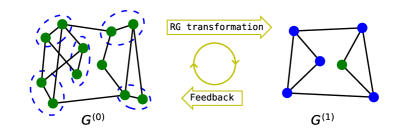
For a graph with the corresponding Hamiltonian , the MQAOA consists of the following steps, which is visualized in Fig. 1.
-
1.
Find a maximal matching of .
-
2.
Perform the QAOA of low depth on to find optimal parameters. In the first round, the initial state is .
-
3.
Prepare the variational state with optimal parameters, and implement measurements to reconstruct reduced density matrix for each pair of qubits connected by edges in , then perform the RG transformation to obtain a new coarse-grained graph and the corresponding Hamiltonian .
-
4.
Find a ground state of .
-
5.
Prepare the quantum state on , which is the initial guessing state for a new round of QAOA.
-
6.
Repeat steps ()-() until the expected energy of converges.
In step (), to find the ground state of on graph , a new MQAOA can be carried out to get an effective graph and the corresponding Hamiltonian through another coarse-grained step. By iterating, a sequence of Hamiltonians is generated until a particular value of is reached, for which can be effectively solved by either a quantum or classical computer. If there is more than one ground state for due to its symmetry, a product state is selected. The selection of a symmetry broken state ensures that the algorithm overcomes the limitation from symmetry protection as proposed in [11]. The initial state in each round is still a tensor product of local states. Depending on the ground state of the next level effective Hamiltonian in the coarse-graining sequence, the qubits connected by an edge in are prepared in one of the two basis vectors, both of which are product states, and the qubits not connected by edges in are prepared in state or . For only single qubit gates are needed, the initial states can be prepared with high precision in NISQ devices.
In the algorithm, there is a competition between the short-distance connection in step () and the long-distance connection in step (), which enables MQAOA to break the locality limitation in a standard QAOA at low depths. Because we need to implement QAOA with a sequence of iterative Hamiltonians, which have different connection scales within the original graph, we have termed the algorithm as multiscale QAOA.
We demonstrate the efficiency of MQAOA using a paradigmatic test: MaxCut problem. The corresponding -qubit problem Hamiltonian is
| (5) |
It is a specific Ising Hamiltonian represented by Eq. (1). We aim to find the state with maximum energy or the ground state of equivalently. As usual, the performance of MaxCut problem is quantified by the approximation ratio defined as the ratio between the maximum variational energy and the maximum exact energy of .
We start by investigating the MaxCut problem on a cycle graph, which is known as the ring of disagrees. It has been studied by numerical computation and theoretical analysis [5, 27, 28]. The optimal approximation ratio achieved by a depth- QAOA for even is bounded above by for all . The exact solution can be obtained with the depth . In the run of MQAOA, each of two adjacent qubits is grouped, and translational symmetry is employed, so the results are applicable for any even integer . Depth- and depth- QAOAs are both tested, and the effective Hamiltonians are exactly solved by classical algorithm after one step of RG transformation. The results are shown in Fig. 2(a). We can observe that both QAOA and RG transformation improve the performance in each round, and near exact solution can be achieved in rounds. As anticipated, depth- QAOA makes convergence faster since applying a QAOA of higher depth should bring the variational state closer to the ground state. We can also observe that the performance ratio of MQAOA converges to much more rapidly than that of the standard QAOA by increasing the depth.
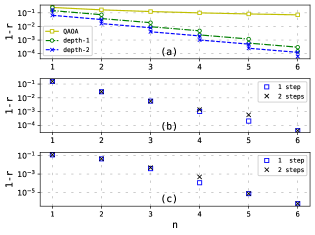
We proceed with considering the problems on two typical families of graphs: random regular graphs and Erdös-Rényi graphs. These graphs are sampled using the NetworkX package. The performance ratios of MQAOA on these graphs are shown in Fig. 2(b-c). For all graphs in the randomly sampled ensemble, the exact solution can be obtained by just adopting depth-1 QAOA in each coarse-graining step. Both one and two steps of coarse-graining are tested. All the performance ratios converge to in approximately rounds, similar to the cycle graphs.
Numerical experiments indicate that the algorithm is prone to get stuck in a suboptimal solution for some graphs when using a depth- QAOA. Increasing the depth of QAOA is an available way to overcome this issue. Nevertheless, we have used an alternative method. It has been discovered by numerical experiments that the performance ratio may rely on a particular partition scheme. Thus, several maximal matchings are tested for the graph in each coarse-graining step to achieve a better solution. To obtain various matchings, the vertices of a graph are randomly shuffled before running the matching searching algorithm. For Hamiltonian with non-integer couplings, it is necessary to have additional considerations to prevent suboptimal results. For example, edges with tiny weights need be excluded before searching for a maximal matching. Because the pair of qubits connected by these edges have little interaction, the subsystem consisting of such a pair of qubits is almost in the maximally mixed state after the first round of QAOA at low depths. Including these edges in the matching would provide little helpful information for coarse-graining.
Computational complexity.
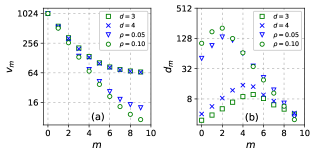
Through successive RG transformations, a sequence of effective graphs with fewer and fewer nodes is built. Numerical simulation evinces that the number of steps of the RG transformation needed is to make the graph size small enough to be solved directly, as shown in Fig. 3(a). We can observe that the decreasing rate of the order of the graph slows down only in the final few steps, where the exact solution is already obtainable. For Erdös-Rényi graphs, especially those with high edge density, the number of vertices is reduced by almost half at each coarse-graining step. For regular graphs, the effective graphs may converge towards a star-shaped graph with a comparatively higher number of vertices, but the ground state of the corresponding Hamiltonian defined on it can be easily solved. In Fig. 3(b), we also display the average degrees of effective graphs, which are related to the vertices involved in the measurement of the local operators in QAOA at each RG coarse-graining step. In summary, if the number of rounds for each effective Hamiltonian in MQAOA is limited to a constant to ensure convergence, and the number of different partition schemes is limited to a constant , then the total number of QAOA runs will be . Our numerical experiments on graphs with varying types and numbers of vertices indicate that is sufficient. Thus, the MQAOA is an efficient algorithm.
Conclusion.
We have proposed the MQAOA to improve the standard QAOA by taking advantage of a real-space RG transformation. The MQAOA enhances performance significantly. It can even solve some particular randomly generated instances exactly. Because just QAOAs at low depths are needed, it does not suffer from barren plateaus and is suitable for NISQ devices to provide a quantum advantage.
This work was supported by the National Natural Science Foundation of China (Grant No. 62371199) and in part by Guangdong Provincial Key Laboratory(Grant No. 2020B1212060066).
References
- [1] Bharti, Kishor and Cervera-Lierta, Alba and Kyaw, Thi Ha and Haug, Tobias and Alperin-Lea, Sumner and Anand, Abhinav and Degroote, Matthias and Heimonen, Hermanni and Kottmann, Jakob S. and Menke, Tim and Mok, Wai-Keong and Sim, Sukin and Kwek, Leong-Chuan and Aspuru-Guzik, Alán. Noisy intermediate-scale quantum algorithms. Reviews of Modern Physics, 94, 015005, 2022.
- [2] Alberto Peruzzo, Jarrod McClean, Peter Shadbolt, Man-Hong Yung, Xiao-Qi Zhou, Peter J. Love, Alán Aspuru-Guzik, and Jeremy L. O’Brien. A variational eigenvalue solver on a photonic quantum processor. Nature Communications, 5(1), July 2014.
- [3] Shantanu Debnath, Norbert M Linke, Caroline Figgatt, Kevin A Landsman, Kevin Wright, and Christopher Monroe. Demonstration of a small programmable quantum computer with atomic qubits. Nature, 536(7614):63, 2016.
- [4] Rami Barends, Alireza Shabani, Lucas Lamata, Julian Kelly, Antonio Mezzacapo, Urtzi Las Heras, Ryan Babbush, Austin G Fowler, Brooks Campbell, Yu Chen, et al. Digitized adiabatic quantum computing with a superconducting circuit. Nature, 534(7606):222, 2016.
- [5] Edward Farhi, Jeffrey Goldstone, and Sam Gutmann. A quantum approximate optimization algorithm. arXiv preprint arXiv:1411.4028, 2014.
- [6] Zhang Jiang, Eleanor G. Rieffel, and Zhihui Wang. Near-optimal quantum circuit for grover’s unstructured search using a transverse field. Phys. Rev. A, 95:062317, Jun 2017.
- [7] Mauro ES Morales, Timur Tlyachev, and Jacob Biamonte. Variational learning of grover’s quantum search algorithm. Physical Review A, 98(6):062333, 2018.
- [8] V. Akshay, H. Philathong, M. E. S. Moracles, and J. D. Biamonte. Reachability deficits in quantum Approximate optimization Physical Review Letters, 124(9):090504, 2020
- [9] Seth Lloyd. Quantum approximate optimization is computationally universal arXiv preprint arXiv:1812.11075, 2018.
- [10] Leo Zhou, Sheng-Tao Wang, Soonwon Choi, Hannes Pichler, and Mikhail D. Lukin. Quantum approximate optimization algorithm: performance, mechanism, and implementation on near-term devices newblockPhysical Review X, 10, 021067, 2020.
- [11] Sergey Bravyi, Alexander Kliesch, Robert Koenig, and Eugene Tang. Obstacles to variational quantum optimization from symmetry protection Physical Review Letters, 125(26):260505, 2020
- [12] Díez-Valle, Pablo and Porras, Diego and García-Ripoll, Juan José. Quantum Approximate Optimization Algorithm Pseudo-Boltzmann States Physical Review Letters, 130, 050601, 2023.
- [13] Edward Farhi, David Gamarnik, Sam Gutmann. The quantum approximate optimization algorithm needs to see the whole graph: a typical case arXiv preprint arXiv:2004.09002, 2020.
- [14] Edward Farhi, David Gamarnik, Sam Gutmann. The quantum approximate optimization algorithm needs to see the whole graph: worst case examples arXiv preprint arXiv:2005.08747, 2020.
- [15] Jarrod R McClean, Sergio Boixo, Vadim N Smelyanskiy, Ryan Babbush, and Hartmut Neven. Barren plateaus in quantum neural network training landscapes. Nature communications, 9(1):4812, 2018.
- [16] Kenneth G. Wilson. The renormalization group: Critical phenomena and the Kondo problem. Reviews of Modern Physics, 47, 773, 1975.
- [17] Steven R. White. Density matrix formulation for quantum renormalization groups. Physical Review Letters, 69(19):2863, 1992
- [18] Steven R. White. Density-matrix algorithms for quantum renormalization groups. Physical Review B, 48, 10345, 1993
- [19] Ulrich Schollwöck. The density-matrix renormalization group. Reviews of Modern Physics, 77, 259, 2005.
- [20] G. Vidal. Entanglement Renormalization Physical Review Letters, 99, 220405, 2007.
- [21] G. Vidal. A class of quantum many-body states that can be efficiently simulated Physical Review Letters, 101, 110501, 2008.
- [22] G. Evenbly, G. Vidal. Algorithms for entanglement renormalization Physical Review B, 79, 144108, 2008.
- [23] Kochenberger, G., Hao, JK., Glover, F. et al. The unconstrained binary quadratic programming problem: a survey J Comb Optim, 28, 58-81, 2014
- [24] Ulrich Schollwöck. The density-matrix renormalization group in the age of matrix product states Annals of Physics, 326, 96, 2011
- [25] Aric A. Hagberg and Daniel A. Schult and Pieter J. Swart. Exploring Network Structure, Dynamics, and Function using NetworkX in Proceedings of the 7th Python in Science Conference, edited by G.Varoquaux, T. Vaught, and J. Millman (Pasadena, CA USA, 2008), pp. 11–15.
- [26] See supplementary material for “Multiscale Quantum Approximate Optimization Algorithm”.
- [27] Zhihui Wang, Stuart Hadfield, Zhang Jiang, and Eleanor G Rieffel. Quantum approximate optimization algorithm for maxcut: A fermionic view. Physical Review A, 97(2):022304, 2018.
- [28] Glen Bigan Mbeng, Rosario Fazio, Giuseppe E. Santoro. Optimal quantum control with digitized Quantum Annealing arXiv preprint quant-ph/1911.12259, 2019.
- [29] Billionnet Alain, Elloumi Sourour. Using a mixed integer quadratic programming solver for the unconstrained quadratic 0-1 problem Math. Program., Ser. A 109, 55–68, 2007.
Supplemental Material for “Multiscale Quantum Approximate Optimization Algorithm”
In this supplemental material, we describe the details of coarse-graining scheme in MQAOA. As noted in the main text, we need to construct a -dimensional subspace from a reduced density matrix of a block consisting of two neighboring qubits, and , with a constraint that three operators should be diagonal with respect to the basis. There three possible forms for the basis: (a) , (b) and (c) , where are quantum states of single qubit and are complex numbers. Only form (a) and (b) are used in MQAOA. An approximate solution for form (a) can be obtained by the following steps, and likewise for form (b).
-
1.
The density matrix is partitioned into blocks .
-
2.
and are diagonalized, , , where are diagonal matrices, , with .
-
3.
is transformed into by unitary operation . The singular value decomposition of the off diagonal block is , with . The first column of is denoted by , and the hermitian conjugate of the first row of is denoted by . The first component of both and are taken as real numbers.
-
4.
To construct 2-dimensional subspace of with basis , the following linear combinations of vectors are taken as an approximate solution: , , where . They are then normalized.
-
5.
and are obtained by unitary transformations: , .
In the loop of MQAOA, we alternate between using form (a) and (b), except in the first round, where we choose the one with smaller .