Concrete Subspace Learning based Interference Elimination for Multi-task Model Fusion

Abstract

Merging models fine-tuned from a common, extensively pre-trained large model but specialized for different tasks has been demonstrated as a cheap and scalable strategy to construct a multi-task model that performs well across diverse tasks. Recent research, exemplified by task arithmetic, highlights that this multi-task model can be derived through arithmetic operations on task vectors. Nevertheless, current merging techniques frequently resolve potential conflicts among parameters from task-specific models by evaluating individual attributes, such as the parameters’ magnitude or sign, overlooking their collective impact on the overall functionality of the model. In this work, we propose the CONtinuous relaxation of disCRETE (Concrete) subspace learning method to identify a common low-dimensional subspace and utilize its shared information to track the interference problem without sacrificing much performance. Specifically, we model the problem as a bi-level optimization problem and introduce a meta-learning framework to find the Concrete subspace mask through gradient-based techniques. At the upper level, we focus on learning a shared Concrete mask to identify the subspace, while at the inner level, model merging is performed to maximize the performance of the merged model. We conduct extensive experiments on both vision domain and language domain, and the results demonstrate the effectiveness of our method. The code is available at https://github.com/tanganke/subspace_fusion

1 Introduction

Pre-trained large models serve as foundational components in machine learning systems nowadays, playing a crucial role. They are adaptive to a wide range of downstream tasks through post fine-tuning, including image classification (He et al., 2016, 2021), natural language processing (Radford et al., 2019; Chung et al., 2022), and speech recognition (Gulati et al., 2020). These fine-tuned models are often specialized for different tasks, and it is desirable to merge them into a unified model that performs well across multiple tasks.

Multi-task model fusion serves as a powerful and scalable methodology for extracting knowledge from individually fine-tuned models targeting different downstream tasks, enabling the construction of a unified multi-task model (Li et al., 2023; Zheng et al., 2023). This approach becomes particularly valuable when access to the underlying training data remains restricted and inaccessible, despite the availability of fine-tuned models(Wu et al., 2019; Tang et al., 2023a). In recent research, exemplified by task arithmetic (Ilharco et al., 2023), a multitude of influential techniques have been introduced to edit pre-trained models and incorporate task-specific models. For a more detailed exploration of these methodologies, please refer to Section 2.

A notable challenge for multi-task model fusion is how to resolve interference between different tasks, which is a phenomenon that occurs when interactions among the parameters from task-specific models negatively impact the performance of the merged multi-task model. Several approaches have been developed to address this issue. For example, Ties-Merging merges task vectors using magnitude trim, elect sign, and disjoint merge strategies instead of simple addition (Yadav et al., 2023). Yu et al. try to address conflicts by randomly dropping parameters and rescaling the remaining parameters in (Yu et al., 2023). However, current merging techniques frequently resolve potential task interference and conflicts among parameters from task-specific models by evaluating individual attributes, such as the parameters’ magnitude or sign, overlooking their collective impact on the overall functionality of the model.

In this study, we introduce the CONtinuous relaxation of disCRETE subspace learning, referred to as Concrete subspace learning in short, to identify a common low-dimensional subspace of model parameter space and effectively leverage the shared information within it to address the issue of task interference, while minimizing the impact on overall performance. In addition, we introduce enhanced variations of two techniques known as Task Arithmetic and AdaMerging, which we’ve termed Concrete Task Arithmetic and Concrete AdaMerging, respectively.

Specifically, we model the problem as a bi-level optimization problem and introduce a meta-learning framework to find the Concrete subspace mask through gradient-based techniques. At the upper level, we focus on learning a shared Concrete mask to identify the subspace, while at the inner level, model merging is performed to maximize the performance of the merged model.

We conduct a wide range of experiments across both the vision and language domains, including scenarios involving fully fine-tuned and LoRA fine-tuned models, as well as experiments on multi-task model fusion and generalization. The experimental results support the efficiency and effectiveness of our approaches.

To summarize, our contributions are as follows:

• We propose the Concrete subspace learning method to identify a common low-dimensional subspace of model parameter space and effectively leverage the shared information within it to address the issue of task interference while minimizing the negative impact on overall performance.

• We model the problem as a bi-level optimization problem and introduce a meta-learning framework to find the Concrete subspace mask through gradient-based techniques.

• We introduce enhanced variations of two multi-task model fusion techniques known as task arithmetic and AdaMerging, which we’ve termed Concrete Task Arithmetic and Concrete AdaMerging, respectively.

• We conduct extensive experiments on both vision domain and language domain. The results demonstrate the effectiveness of our method.

2 Related Work

In practical applications, it is common practice to fine-tune a pre-trained model on a diverse set of downstream tasks. The fine-tuned models are often specialized for different tasks, and it is desirable to merge them into a unified model that performs well across multiple tasks, this is referred to as multi-task model fusion in the literature (Li et al., 2023; Zheng et al., 2023). Multi-task model fusion is a powerful and scalable methodology for extracting knowledge from individually task-specific models and construction of a unified multi-task model. This is particularly valuable when access to the underlying training data remains privately restricted or inaccessible. In recent research, innovative approaches have been explored to understand and improve the integration of various task-specific models.

Mode connectivity. One notable concept in this area is mode connectivity, where research (Daniel Freeman and Bruna, 2017; Nagarajan and Kolter, 2019) has demonstrated that solutions found through gradient-based optimization can be interconnected through a path in the weight space, termed mode connectivity (Draxler et al., 2019; Entezari et al., 2022). This insight allows for the discovery of models suited for fusion that lie along paths of low loss. Strategies for mode connectivity vary, with some researchers exploring linear mode connectivity (LMC) (Garipov et al., 2018) and others delving into non-linear paths (Tatro et al., 2020) or connectivity within a low-dimensional subspace (Yunis et al., 2022).

Weight interpolation. The most straightforward method for multi-task model fusion could be weight interpolation (Matena and Raffel, 2022). This technique merges multiple models into a unified model without requiring exhaustive computations or prior optimization. Aggregation can be direct or performed within a subspace. Approaches such as Model soups (Wortsman et al., 2022), Task Arithmetic (Ilharco et al., 2023), and stochastic weight averaging (Kaddour, 2022; Izmailov et al., 2019) have been shown to enhance performance effectively. However, biases may arise when models of significantly different architectures or parameter quantities are normalized and merged, a challenge that remains to be fully addressed.

Alignment. Another technique is alignment (Li et al., 2016; Tatro et al., 2020), which involves matching and averaging units across different models. This process narrows the mathematical distances, such as Euclidean distances, between models, harmonizing them for more effective fusion(George Stoica et al., 2023; Jin et al., 2023). It includes methods such as activation matching and weight matching and extends to concepts like Re-basin (Ainsworth et al., 2023), which utilizes permutation invariance to bring solutions into a single low-loss basin.

Multi-task model fusion under PEFT setting. As the size of the models continues to grow, the cost of performing full fine-tuning also increases. Therefore, parameter-efficient fine-tuning methods are gaining more attention. In addition to merging fully fine-tuned models, some researchers have explored the fusion of models that are parameter-efficiently fine-tuned. For example, apply weight interpolation on the parameter space of adapter modules (Chronopoulou et al., 2023; Huang et al., 2023; Zhang et al., 2023), based on the Fisher information matrix, Wu et al. compute similarity among tasks, subsequently, select adapter modules, and interpolate weights (Wu et al., 2023), or improve the performance of model fusion by partially linearizing the PEFT modules (Tang et al., 2023b).

Unlike previous research, our study specifically addresses the problem of task interference in multi-task model fusion. Our proposed method acts as a highly adaptable add-on to existing model fusion techniques and can be applied to both fully fine-tuned models and parameter-efficiently fine-tuned models. In this paper, we present enhanced variations of two techniques known as Task Arithmetic and AdaMerging, which we’ve termed Concrete Task Arithmetic and Concrete AdaMerging, respectively.

3 Methodology

In this section, we first introduce the problem setting and the notations used in this paper. Then we present the Concrete subspace learning, which is a novel method to meta-learn a shared subspace across tasks and perform model fusion. Finally, we briefly discuss the test-time adaptation.

3.1 Preliminary

We start with a pre-trained neural network $f$ parameterized by $\theta_{0}\in\mathbb{R}^{d}$, trained on an extensive dataset, and a set of $n$ downstream tasks $\mathcal{S}=\{s_{i}\}_{i=1}^{n}$. Subsequently, the pre-trained model $f$ undergoes fine-tuning on each task $s_{i}$ to obtain a fine-tuned model parameterized by $\theta_{i}$. Specifically, the task vector is defined as $\tau_{i}=\theta_{i}-\theta_{0}$, this definition is first introduced in (Ilharco et al., 2023) and enables us to focus on the task-specific information. Given access to both the pre-trained model weights and these fine-tuned model weights, our objective is to merge these models into a unified model capable of performing effectively on all tasks within $\mathcal{S}$.

3.2 An Overview of Concrete Subspace Learning

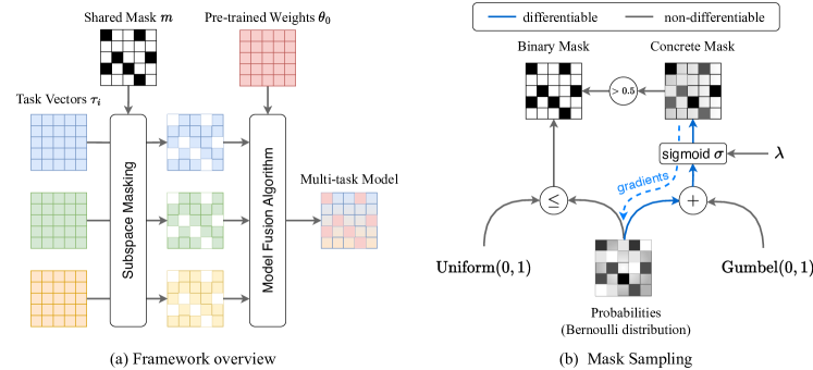
Figure 1: (a) Framework overview. Our proposed framework comprises two main steps: first, establishing a common subspace for task vectors across various tasks using a shared mask, and second, merging the models within this shared subspace. (b) Mask sampling. Here we illustrate the procedure for sampling discrete binary masks and our differentiable Concrete mask. It’s important to note that while a Concrete mask can also be binarized, this binarization process is non-differentiable.

To address the aforementioned problem, we propose a Concrete subspace learning method to identify a common subspace across tasks and utilize the shared information in it to track the interference problem without sacrificing much performance. We model the problem of identifying this common low-dimensional subspace across tasks as a bi-level optimization problem and design an algorithm to meta-learn the shared mask that is beneficial across multiple tasks. Mathematically, we can express the problem as

$$\max_{m}\max_{w}\frac{1}{n}\sum_{i}^{n}\text{Score}\left(\mathcal{A}(\theta_{0},\{\mathcal{M}(\tau_{j},m)\}_{j=1}^{n},w),s_{i}\right).$$ (1)

Where $m\in\mathbb{R}^{d}$ is the shared mask to be found, $\mathcal{A}$ is a model fusion algorithm associated with algorithm parameters $w$, $\mathcal{M}:\mathbb{R}^{d}\times\mathbb{R}^{d}\mapsto\mathbb{R}^{d}$ is the Concrete mask process introduced in the next subsection, and Score is the task-specific evaluation metric. The upper level objective is to find a shared mask $m$ that maximizes the performance of the merged model $\mathcal{A}(\theta_{0},\{\mathcal{M}(\tau_{j},m)\}_{j=1}^{n},w)$ across all tasks. The objective at the inner level is to find the optimal algorithmic parameters $w$ that maximize the performance of the merged model on each task. Figure 1(a) illustrates the framework of our proposed Concrete subspace learning. We first learn a shared subspace across tasks by learning a shared mask $\mathbf{m}$, and then we merge the models within this shared subspace.

Algorithm 1 Meta-Learning a shared Concreate mask across tasks

1: Input:

1. a pre-trained model $f$ parameterized by $\theta_{0}$,

2. a set of fine-tuned task vectors $\mathcal{T}=\{\tau_{i}\}_{i=1}^{n}$,

3. a set of target tasks $\mathcal{S^{\text{test}}}$ (unlabeled data).

2: Output: a shared Concreate mask $\mathbf{m}$ parameterized by logits $\mathbf{x}$.

3:Initialize the logits $\mathbf{x}$ to zeros until convergence

4:mask task vectors $\mathcal{T}$ with $\mathbf{m}$ to get $\mathcal{T}^{\prime}$

5:rescale the masked task vectors $\mathcal{T}^{\prime}$ to get $\mathcal{T}^{\prime\prime}$

6:initialize parameter $w$ associated with model fusion algorithm

7:$\theta\leftarrow\text{MergeWeight}(\theta_{0},\mathcal{T}^{\prime\prime};w)$ $\triangleright$ such as Task Arithmetic, AdaMerging or ModelSoups $w$ is optimizable each task $s_{i}\in\mathcal{S}^{\text{test}}$

8:sample a batch of unlabeled data $\mathcal{D}_{i}$ from $s_{i}$

9:$l_{i}\leftarrow\mathcal{L}_{i}(f(\theta),\mathcal{D}_{i})$ $\triangleright$ unsupervised loss such as entropy loss for TTA

10:$w^{\prime}\leftarrow w-\alpha\nabla_{w}\left(\sum_{i=1}^{n}l_{i}\right)$

11:$\theta\leftarrow\text{MergeWeight}(\theta_{0},\mathcal{T}^{\prime\prime};w^{\prime})$ $\triangleright$ update merged weights with the updated $w^{\prime}$ each task $s_{i}\in\mathcal{S}$

12:sample a batch of unlabeled data $\mathcal{D}_{i}$ from $s_{i}$

13:$l_{i}\leftarrow\mathcal{L}_{i}(f(\theta),\mathcal{D}_{i})$ $\triangleright$ unsupervised loss such as entropy loss for TTA

14:$\mathbf{x}\leftarrow\mathbf{x}-\beta\nabla_{\mathbf{x}}\left(\sum_{i=1}^{n}l_{i}\right)$

15:Return: the Concrete mask paramemetized by logits $\mathbf{x}$.

Algorithm 2 Concrete Task Arithmetic

1: Input:

1. a Concrete mask $\mathbf{m}$,

2. pre-trained model weights $\theta_{0}$,

3. a set of fine-tuned task vectors $\mathcal{T}=\{\tau_{i}\}_{i=1}^{n}$,

4. a single scaling coefficient $\lambda$.

2: Output: merged weights $\theta$.

3:mask task vectors $\mathcal{T}$ with $\mathbf{m}$ to get $\mathcal{T}^{\prime}$

4:rescale the masked task vectors $\mathcal{T}^{\prime}$ to get $\mathcal{T}^{\prime\prime}=\{\tau^{\prime\prime}_{i}\}_{i=1}^{n}$

5:add up the scaled task vectors $\tau^{\prime\prime}_{i}$ to obtain $\tau^{*}$

6:$\theta\leftarrow\theta_{0}+\lambda\tau^{*}$ $\triangleright$ merge the weights

7:Return: merged weights $\theta$.

Algorithm 3 Concrete AdaMerging

1: Input:

1. a Concrete mask $\mathbf{m}$,

2. pre-trained model weights $\theta_{0}$,

3. a set of fine-tuned task vectors $\mathcal{T}=\{\tau_{i}\}_{i=1}^{n}$,

4. task-wise weights $\mathbf{\lambda}=\{\lambda_{i}\}_{i=1}^{n}$ (or layer-wise weights $\{\lambda_{i}^{l}\}_{i=1,l=1}^{n,L}$).

2: Output: merged weights $\theta$.

3:mask task vectors $\mathcal{T}$ with $\mathbf{m}$ to get $\mathcal{T}^{\prime}$

4:rescale the masked task vectors $\mathcal{T}^{\prime}$ to get $\mathcal{T}^{\prime\prime}=\{\tau^{\prime\prime}_{i}\}_{i=1}^{n}$

5:optimize $\mathbf{\lambda}$ on unlabeled test data (Yang et al., 2023)

6:merge model weights as Eq.(16)

7:Return: merged weights $\theta$.

Algorithm 1 provides a detailed demonstration of meta-learning a shared mask across tasks. Given a pre-trained model, fine-tuned task vectors, and a set of source or target tasks, the algorithm iteratively refines a Concrete mask parameterized by its logits $\mathbf{x}$. In the inner loop, we first optimize the parameters of a model fusion algorithm (like the task-wise or layer-wise weight parameters of AdaMerging) on unlabeled test data in a test-time adaptation manner, and then merge the model weights with the updated parameters. Then, in the outer loop, we optimize the logits $\mathbf{x}$ of the Concrete mask $\mathbf{m}$ to find a shared subspace that is beneficial across tasks.

Our approach functions as a versatile plug-in method, seamlessly integrable with various model fusion techniques. Algorithm 2 and Algorithm 3 provide detailed demonstrations of how our approach can be combined with Task Arithmetic and AdaMerging, respectively. We refer to the combination of our method with these techniques as “Concrete Task Arithmetic” and “Concrete AdaMerging”, highlighting the specific adaptations and enhancements resulting from the incorporation of our approach.

3.3 The Concrete Masking Process

For a neural network, we can use a shared mask $\mathbf{m}$ to identify a subspace of the parameter space $\mathbf{\theta}$ by setting the parameters that are not in the subspace to zero, i.e. $\mathbf{\theta}\circ\mathbf{m}$, where $\circ$ denotes the element-wise product operation. However, in our study, since our focus lies on the task-specific knowledge of fine-tuned models, we perform this operation on the task vector $\tau^{\prime}_{i}=\tau_{i}\circ\mathbf{m}$. Following this operation, we rescale the remaining parameters of the task vector. Specifically, we divide them by the mean value of the mask entries to obtain the final task vector

$$\tau^{\prime\prime}_{i}=\frac{\tau^{\prime}_{i}}{\mathbb{E}_{m\sim\mathbf{m}}[m]}=\frac{\tau_{i}\circ\mathbf{m}}{\mathbb{E}_{m\sim\mathbf{m}}[m]}.$$ (2)

This rescale trick has also been employed in (Yu et al., 2023), which has been shown to be effective in maintaining the performance of the fine-tuned models. Without this operation, the fine-tuned models would be significantly degraded, as the mask would be too sparse to retain the task-specific information.

A binary mask can be drawn from a Bernoulli distribution denoted by $\text{Bernoulli}(\mathbf{p}=\sigma(\mathbf{x}))$, where $\mathbf{p}$ is the probability (and $\mathbf{x}$ denotes the logits) of each parameter being activated. The left portion of Figure 1(b) illustrates the process of generating discrete binary masks by sampling from a uniform distribution and comparing the samples with probabilities. Alternatively, the Gumbel-Max trick can be employed to treat the Bernoulli distribution as a 2-class categorical distribution for sampling. However, regardless of the method used, the discrete Bernoulli distribution is not differentiable, preventing the backpropagation of gradients through it to optimize the parameters $\mathbf{p}$ or $\mathbf{x}$.

Inspired by (Maddison et al., 2017; Jang et al., 2017), we use a continuous relaxation of the discrete Bernoulli distribution to represent the mask to identify the common subspace. The right portion of Figure 1(b) illustrates the procedure for generating our differentiable Concrete mask. We can consider the Bernoulli random variables as a special 2-class case of the Gumbel-Softmax random variables, which are continuous relaxations of the discrete Categorical random variables. We provide a more detailed explanation of the Gumbel-Max trick, Concrete random variables, and Gumbel-Softmax distribution in Appendix A.

Let $p_{0}$ and $p_{1}$ denote the unnormalized probabilities of a Bernoulli random variable being 0 and 1, respectively, with $x$ representing the logits. Then, the probability of the event $m=1$ is given by

$$\mathbb{P}(m=1)=\frac{p_{1}}{p_{0}+p_{1}}=\sigma(x),$$ (3)

where $\sigma$ denotes the sigmoid function. In the context of the Gumbel-Max trick, the occurrence of the event $m=1$ is determined by the condition $g_{1}+\log p_{1}>g_{0}+\log p_{0}$, where $g_{0}$ and $g_{1}$ are two independent standard Gumbel random variables. Thus, we have

$$\mathbb{P}(m=1)=\mathbb{P}(g_{1}+\log p_{1}>g_{0}+\log p_{0})=\mathbb{P}\left((g_{1}-g_{0})+(\log p_{1}-\log p_{0})>0\right).$$ (4)

Because the difference of two standard Gumbel random variables is a Logistic random variable, we can replace $g_{1}-g_{0}$ by $\log u-\log(1-u)$ where $u$ is a random variable sampled from a uniform distribution on the interval $(0,1)$. Substitute this into Eq.(4) and express the probability in terms of the logits $x$ to simplify the expression, we have

$$\mathbb{P}(m=1)=\mathbb{P}\left(\log\frac{u}{1-u}+\log\frac{\sigma(x)}{1-\sigma(x)}>0\right),\quad u\sim\text{Uniform}(0,1).$$ (5)

The binary Concrete distribution offers a continuous relaxation of the discrete Bernoulli random variables, which is beneficial for gradient-based optimization as it allows for the backpropagation of gradients even through the sampling process. Instead of making a hard decision as Eq.(5), we use a temperature parameter $\lambda$ to control the steepness of the sigmoid function, and hence control how close our ‘soft’ decisions are to being ‘hard’ decisions. The continuous version of the Bernoulli random variable is then given by

$$\hat{m}=\sigma\left(\left(\log\frac{u}{1-u}+\log\frac{\sigma(x)}{1-\sigma(x)}\right)/\tau\right).$$ (6)

Definition 1 (Concrete mask)

A Concrete mask, denoted as $\mathbf{m}$, is a $d$-dimensional real vector in $[0,1]^{d}$ parameterized by logits $\mathbf{x}\in\mathbb{R}^{d}$ or probabilities $\mathbf{p}=\sigma(\mathbf{x})$, where $d$ is the number of parameters in a neural network. Each entry $m_{i}$ of the mask is a random variable sampled from a Concrete distribution as Eq.(6).

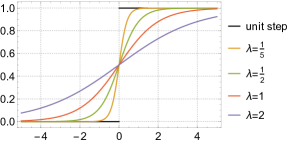
Figure 2: The sigmoid function $\sigma(\cdot/\lambda)$ with different temperatures $\lambda$.

As the temperature $\lambda$ approaches zero, the sigmoid function becomes a step function, and the Concrete random variable $\hat{m}$ becomes a Bernoulli random variable, as shown in Figure 2. In the limit when $\lambda\to 0$, this results in sampling $m=1$ if $\log\frac{\sigma(x)}{1-\sigma(x)}>-\log\frac{u}{1-u}$, consistent with the original Gumbel-Max trick. The binary Concrete distribution thus provides a differentiable approximation to Bernoulli random variables. In addition to the Concrete mask sampling, we can further binarize the Concrete mask by setting the entries with values greater than 0.5 to 1 and the rest to 0.

3.4 Test-Time Adaptation

In this section, we discuss a situation wherein the target dataset is exclusively composed of unlabeled test data. This implies that our objective is centered around the concept of test-time adaptation, where the focus is on adapting and refining the merged model’s performance specifically during the testing phase (Mounsaveng et al., 2023; Liang et al., 2023). In this context, the emphasis lies on optimizing the model’s predictions and generalization ability when confronted with unseen, unlabeled instances during the testing process.

Take classification tasks as an example. We can use the merged model to make predictions on the unlabeled test data, and then use the predictions to optimize the merged model. Specifically, we can use the entropy loss to optimize the merged model, which is defined as

$$\mathcal{L}_{\text{entropy}}=\mathbb{E}[-\log p(\hat{y}|x)]=-\frac{1}{n}\sum_{i=1}^{n}\sum_{j=1}^{C}p(\hat{y}_{c}|x_{i})\log p(\hat{y}_{c}|x),$$ (7)

where $x_{i}$ is the $i$-th unlabeled instance, $p(\hat{y}_{c}|x_{i})$ is the predicted probability of the $c$-th class, and $C$ is the number of classes. By minimizing the entropy loss on the unlabeled test data, the model tends to make confident predictions.

4 Experiments

In this section, we conduct experiments across diverse tasks on both vision and language domains to demonstrate the effectiveness of our proposed method. We utilize pre-trained CLIP (Radford et al., 2021a) for vision tasks and pre-trained Flan-t5 (Chung et al., 2022) for language tasks. Please refer to Appendix B for detailed descriptions of the pre-trained models, downstream tasks, and fine-tuning procedures.

We compare our approach with simple averaging (Wortsman et al., 2022), task arithmetic (Ilharco et al., 2023), Ties-Merging (Yadav et al., 2023), and AdaMerging (Yang et al., 2023). To facilitate a comprehensive comparison of various methods, we categorize them into three groups: task arithmetic-based, AdaMerging-based and others. Task arithmetic-based methods involve constructing a merged task vector, subsequently scaled by a factor, and added to the pre-trained model. In contrast, AdaMerging-based methods allocate distinct task-wise or layer-wise weights to each task vector. This categorization is evident in the table presentation. A more detailed description of the baseline methods is provided in Appendix C.1. Appendix C.2 and Appendix C.3 offer additional insights into task arithmetic-based and AdaMerging-based methods, respectively, delving into their experimental results.

4.1 Vision Tasks

For vision tasks, we utilize CLIP-ViT-B/32 and CLIP-ViT-L/14 as our pre-trained model and conduct our experiments on eight image classification tasks. These tasks are SUN397 (Xiao et al., 2010), Stanford Cars (Krause et al., 2013), RESISC45 (Cheng et al., 2017), EuroSAT (Helber et al., 2018), SVHN (Netzer et al., 2021), GTSRB (Stallkamp et al., 2012), MNIST (Lecun et al., 1998) and DTD (Cimpoi et al., 2014). We report top-1 accuracy as a performance metric.

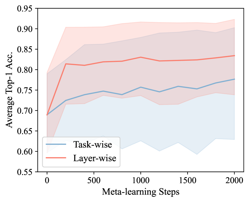
(a) Meta-learn the Concrete mask

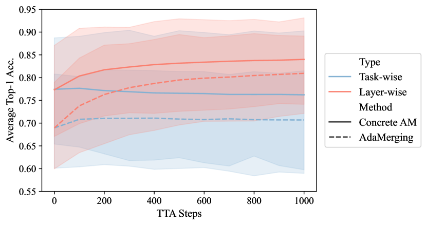
(b) Comparing AdaMerging with and without the Concrete mask

Figure 3: Performance comparison between AdaMerging and Concrete AdaMerging. Here we show the whole process of applying AdaMerging and Concrete AdaMerging to CLIP-ViT-B/32, the y-axes are shared by these two subfigures: (a) shows the performance of the merged model during the meta-learning phase of the Concrete AdaMerging, see Algorithm 1; (b) illustrates the comparison between AdaMerging with and without the Concrete mask.

Table 1: Multi-task performance when merging CLIP-ViT-B/32 models on all eight tasks.

Method	SUN397	Cars	RESISC45	EuroSAT	SVHN	GRSRB	MNIST	DTD	Avg.
Individual	75.3	77.7	96.1	99.9	97.5	98.7	99.7	79.4	90.5
Traditional MTL	73.9	74.4	93.9	98.2	95.8	98.9	99.5	77.9	88.9
Weight Averaging	65.3	63.3	71.4	73.6	64.2	52.8	87.5	50.1	66.0
Fisher Merging	68.6	69.2	70.7	66.4	72.9	51.1	87.9	59.9	68.3
RegMean	65.3	63.5	75.6	78.6	78.1	67.4	93.7	52.0	71.8
Task Arithmetic (TA)-Based
Task Arithmetic	55.3	54.9	66.7	77.4	80.2	69.7	97.3	50.1	69.0
Ties-Merging	65.0	64.3	74.7	76.8	81.3	69.4	96.5	54.3	72.8
Concrete TA	62.5	61.1	76.0	95.7	91.0	81.9	98.5	51.9	77.3
Task-wise AdaMerging (TW AM)-Based
TW AM	58.3	53.2	71.8	80.1	81.6	84.4	93.4	42.7	70.7
TW AM++	60.8	56.9	73.1	83.4	87.3	82.4	95.7	50.1	73.7
TW Concrete AM	62.7	58.9	74.5	94.8	91.1	95.0	98.1	34.6	76.2
Layer-wise AdaMergin (LW AM)-Based
LW AM	64.2	69.5	82.4	92.5	86.5	93.7	97.7	61.1	80.9
LW AM++	66.6	68.3	82.2	94.2	89.6	89.0	98.3	60.6	81.1
LW Concrete AM	67.8	70.0	87.5	96.0	91.6	96.7	98.7	63.8	84.0

Table 2: Multi-task performance when merging CLIP-ViT-L/14 models on all eight tasks.

Method	SUN397	Cars	RESISC45	EuroSAT	SVHN	GRSRB	MNIST	DTD	Avg.
Individual	82.3	92.4	97.4	99.9	98.1	99.2	99.7	84.1	94.1
Traditional MTL	80.8	90.6	96.3	96.3	97.6	99.1	99.6	84.4	93.5
Weight Averaging	72.1	81.6	82.6	91.4	78.2	70.6	97.0	62.8	79.5
Fisher Merging	69.2	88.6	87.5	93.5	80.6	74.8	93.3	70.0	82.2
RegMean	73.3	81.8	86.1	97.0	88.0	84.2	98.5	60.8	83.7
Task Arithmetic (TA)-Based
Task Arithmetic	82.1	65.6	92.6	86.8	98.9	86.7	74.1	87.9	84.4
Ties-Merging	84.5	67.7	94.3	82.1	98.7	88.0	75.0	85.7	84.5
Concrete TA	86.2	66.9	96.7	93.4	99.1	89.0	74.6	93.6	87.4
Layer-wise AdaMergin (LW AM)-Based
LW AM	79.0	90.3	90.8	96.2	93.4	98.0	99.0	79.9	90.8
LW AM++	79.4	90.3	91.6	97.4	93.4	97.5	99.0	79.2	91.0
LW Concrete AM	77.8	91.2	92.1	97.0	94.4	97.9	99.0	79.5	91.1

Multi-task model fusion experiments. We first conduct multi-task model fusion experiments on CLIP-ViT-B/32 and CLIP-ViT-L/14. The obtained results are detailed in Table 1 and Table 2 correspondingly. Notably, our proposed methodologies, Concrete Task Arithmetic and Concrete AdaMerging, consistently outperform alternative methods across the majority of tasks. The layer-wise Concrete AdaMerging surpasses all other Multi-task model fusion methods and is only second to traditional multi-task learning. Furthermore, within their respective comparison groups, they achieve the highest average performance.

Among the three Task Arithmetic-based methods, Concrete Task Arithmetic stands out, achieving the highest performance in five out of eight tasks for CLIP-ViT-B/32 and seven out of eight tasks for CLIP-ViT-L/14. Moreover, within the AdaMerging-based methods, Layer-wise Concrete AdaMerging showcases remarkable effectiveness by attaining the top performance in all eight tasks for CLIP-ViT-B/32 and three out of eight tasks for CLIP-ViT-L/14. These findings underscore the robust effectiveness of our proposed methodologies in the context of multi-task model fusion. We provide a more detailed analysis of Task Arithmetic-based and AdaMerging-based methods in Appendix C.2 and Appendix C.3. These appendices offer a comprehensive exploration and discussion of their experimental results.

Figure 3 provides a visual representation of the performance contrast between AdaMerging and Concrete AdaMerging. Specifically, Figure 3(a) presents the performance of the merged model during the meta-learning phase of Concrete AdaMerging, while Figure 3(b) illustrates the comparison between AdaMerging with and without the Concrete mask.

As shown in Figure 3(a), the performance of the merged model gradually increases during the meta-learning phase of Concrete AdaMerging, indicating that the Concrete mask is capable of capturing the shared information among tasks. Furthermore, Figure 3(b) demonstrates that the Concrete mask can effectively alleviate the interference problem, as the performance of the merged model with the Concrete mask is consistently higher than that of the merged model without the Concrete mask.

Table 3: Generalization results on two unseen tasks when merging ViT-B/32 models on six tasks.

Method	Seen Tasks							Unseen Tasks
	SUN397	Cars	RESISC45	DTD	SVHN	GTSRB	Avg.	MNIST	EuroSAT	Avg.
Task Arithmetic	63.4	62.3	75.3	57.8	84.7	80.4	70.7	77.3	45.6	61.4
Ties-Merging	67.8	66.2	77.0	56.2	77.2	71.0	69.2	75.9	43.1	59.5
Concrete TA	66.2	66.4	82.0	58.3	91.4	92.7	72.9	80.7	52.9	66.8
AdaMerging	65.2	65.9	88.5	61.1	92.2	91.5	77.4	84.0	56.1	70.0
AdaMerging++	68.2	67.6	86.3	63.6	92.6	89.8	78.0	83.9	53.5	68.7
Concrete AM	68.9	71.7	91.2	66.9	94.1	97.5	81.7	83.6	53.9	69.7

Method	Seen Tasks							Unseen Tasks
	SUN397	Cars	GTSRB	EuroSAT	DTD	MNIST	Avg.	RESISC45	SVHN	Avg.
Task Arithmetic	63.8	63.9	75.2	87.3	56.6	95.7	73.8	52.5	49.9	51.2
Ties-Merging	67.8	67.2	67.8	78.9	56.2	92.8	71.8	58.4	49.3	53.9
Concrete TA	66.4	65.7	90.0	96.4	57.2	98.1	79.0	54.3	58.9	56.6
AdaMerging	67.1	67.8	94.8	94.4	59.6	98.2	80.3	50.2	60.9	55.5
AdaMerging++	68.9	69.6	91.6	94.3	61.9	98.7	80.8	52.0	64.9	58.5
Concrete AM	69.6	71.0	97.6	97.3	68.7	99.0	83.9	48.1	62.3	55.2

Generalization experiments. We also carry out generalization experiments on CLIP-ViT-B/32. For this analysis, we designate two tasks as unseen, while the remaining six tasks are considered seen. The experiments involve merging the CLIP-ViT-B/32 models fine-tuned on the six seen tasks, and we evaluate the performance of the merged model on both the seen and unseen tasks. The outcomes from two independent runs of the generalization experiments are detailed in Table 3.

As shown in Table 3, both Concrete Task Arithmetic and Concrete AdaMerging demonstrate superior performance over a range of alternative techniques for a majority of the tasks assessed. In the first set of experiments, Concrete outperformed other task arithmetic-based methods in seven out of eight tasks, while in both sets, Concrete AdaMerging surpassed other methods in six out of eight tasks. On unseen tasks, Concrete Task Arithmetic significantly outperforms other task arithmetic-based methods. This indicates that the learned Concrete mask can effectively capture the shared information between different tasks. This is helpful for transfering knowledge from seen tasks to unseen tasks.

4.2 Language Tasks

For language tasks, we utilize Flan-T5-base and Flan-T5-large as our pre-trained models and conduct our experiments on eight NLP tasks from GLUE benchmark (Wang et al., 2018). We report Spearman’s $\rho$ for STSB and accuracy for others.

Table 4: Multi-task performance when merging Flan-T5-base (LoRA fine-tuned) models on all eight tasks.

Method	CoLA	MNLI	MRPC	QNLI	QQP	RTE	SST2	STSB	Avg.
Individual	69.1	82.7	85.5	90.9	84.0	84.4	92.9	87.4	84.6
Weight Averaging	69.7	59.7	78.9	90.1	83.8	80.5	91.2	72.0	78.2
Task Arithmetic (TA)-Based
Task Arithmetic	68.8	55.2	78.7	89.8	83.7	79.1	91.5	72.4	77.4
Ties-Merging	68.3	56.3	79.4	89.8	83.7	79.4	91.6	71.2	77.5
Concrete TA	69.1	58.1	78.4	89.9	83.5	79.4	91.6	73.4	78.0
Layer-wise AdaMergin (LW AM)-Based
LW AM	69.1	60.3	78.4	90.0	83.6	79.1	91.6	74.1	78.3
LW Concrete AM	69.0	59.4	80.1	89.9	82.9	79.1	91.7	75.4	78.5

Table 5: Multi-task performance when merging Flan-T5-large (LoRA fine-tuned) models on all eight tasks.

Method	CoLA	MNLI	MRPC	QNLI	QQP	RTE	SST2	STSB	Avg.
Individual	80.2	88.5	89.2	94.4	87.2	91.7	95.2	90.9	89.6
Weight Averaging	74.6	84.3	84.1	92.8	86.3	87.4	94.8	88.0	86.5
Task Arithmetic (TA)-Based
Task Arithmetic	76.9	85.4	85.3	93.9	85.8	88.1	95.2	87.8	87.3
Ties-Merging	77.1	85.1	86.3	93.9	86.0	87.7	95.1	88.0	87.4
Concrete TA	76.6	86.4	86.0	93.9	85.9	88.4	95.2	87.9	87.5
Layer-wise AdaMergin (LW AM)-Based
LW AM	76.7	87.6	84.8	93.8	85.9	88.1	95.2	88.6	87.6
Concrete LW AM	76.1	87.7	85.5	93.8	85.9	88.1	95.4	87.1	87.5

Multi-task model fusion experiments. Similar to the experiments on vision tasks, we conduct multi-task model fusion experiments on LoRA fine-tuned Flan-T5-base and Flan-T5-large. The hyperparameter settings and other details about model fine-tuning, model fusion, and evaluation are provided in Appendix B, C and Appendix D.1. The results are detailed in Table 4 and Table 5 correspondingly. As shown in tables, our proposed methodologies, the “Concrete” version of Task Arithmetic and layer-wise AdaMerging, appear to offer incremental advantages.

We also observed that the effectiveness of our Concrete methods on LoRA fine-tuned language models wasn’t significantly more pronounced when compared to other methods. This can be attributed to two factors:

On one hand, pre-trained large language models inherently possess a commendable capacity for multitasking. These advanced models come equipped with the inherent ability to efficiently process and excel across a diverse range of tasks. Consequently, the potential for substantial improvement through any specialized method may be constrained, given the already robust performance of these models. On the other hand, in comparison to full fine-tuning, LoRA fine-tuning can be considered as a form of subspace fine-tuning. Therefore, in this scenario, the benefits of further seeking smaller subspaces are likely to be constrained.

5 Conclusion

In this work, we proposed the CONtinuous relaxation of disCRETE (Concrete) subspace learning method. This subspace learning-based strategy identifies a common low-dimensional subspace and uses the shared information within it to address the issue of task interference in multi-task model fusion, without significantly impacting overall performance. We also present enhanced extensions of two techniques known as task arithmetic and AdaMerging, which we’ve termed Concrete Task Arithmetic and Concrete AdaMerging, respectively.

Compared to previous algorithms, our method offers the advantage of effectively resolving task interference by considering the collective impact of parameters from task-specific models, rather than evaluating individual naive attributes like the parameters’ magnitude or sign. This is achieved through our proposed meta-learning framework.

Our extensive experiments in both the vision and language domains demonstrated the effectiveness of our method across a wide range of tasks. While our method effectively addresses task interference and maintains overall performance, it does require the computation of a bi-level optimization problem. This may increase computational time. Future work could further explore the use of zero-order optimization techniques to reduce the memory footprint of our algorithm, thereby enhancing its scalability on larger models.

Appendix A Contrete Masking

A.1 The Gumbel-Max Trick

Consider a discrete categorical distribution parameterized by logits $\mathbf{x}=(x_{1},\dots,x_{n})\in\mathbb{R}^{n}$, where $x_{i}$ is the logit of the $i$-th category. The Gumbel-Max trick [Gumbel, 1954, Luce, 1959, Maddison et al., 2014] states a reparameterization trick to sample from the categorical distribution by sampling from the standard Gumbel distribution $\text{Gumbel}(\mu=0,\beta=1)$ and taking the argmax of the sum of the Gumbel random variables and the logits.

This trick proceeds as follows: sample $n$ Gumbel random variables $g_{1},\dots,g_{n}$ independently from the standard Gumbel distribution $\text{Gumbel}(\mu=0,\beta=1)$ , find the index $i$ of that maximizes $x_{i}+g_{i}$, then we have

$$\operatorname*{arg\,max}_{i\in[n]}(x_{i}+g_{i})\sim\text{Categorical}(\text{softmax}(\mathbf{x})).$$ (8)

If we represent the categorical distribution as a one-hot vector $\mathbf{y}=(y_{1},\dots,y_{n})\in\{0,1\}^{n}$, where $y_{i}=1$ indicates that the $i$-th category is sampled and for all $j\neq i$, $y_{j}=0$, then we have

$$\mathbb{P}(y_{k}=1)=\mathbb{P}\left(\operatorname*{arg\,max}_{i\in[n]}(x_{i}+g_{i})=k\right)=\frac{\exp(x_{k})}{\sum_{i=1}^{n}\exp(x_{i})}.$$ (9)

A.2 Continuous Relaxation of the discrete Categorical Distribution

Since the derivative of the $\operatorname*{arg\,max}$ function is not defined, we cannot backpropagate the gradients through it. To address this issue, [Maddison et al., 2017] proposed to use a continuous relaxation of the discrete categorical distribution. A CONCRETE random variable (CONtinuous relaxation of disCRETE random variable) relax the condition that the one-hot vector $\mathbf{y}$ must be located at the vertices of the $(n-1)$-dimensional simplex $\Delta^{n-1}$, and instead, it allows $\mathbf{y}$ to be located anywhere inside the simplex $\Delta^{n-1}$, i.e. $\{y\in\mathbb{R}^{n}|y_{i}\in[0,1],\sum_{i=1}^{n}y_{i}=1\}$.

To sample a Concrete random variable $\mathbf{y}$ from a distribution that is parameterized by a temperature hyperparameter $\lambda>0$ and a vector of logits $\mathbf{x}=(x_{1},\dots,x_{n})\in\mathbb{R}^{n}$, we have

$$\mathbf{y}=\text{softmax}\left(\frac{\mathbf{x}+\mathbf{g}}{\lambda}\right),\quad y_{i}=\frac{\exp\left((x_{i}+g_{i})/{\lambda}\right)}{\sum_{j=1}^{n}\exp\left(({x_{j}+g_{j}})/{\lambda}\right)}\quad\text{for}\,\,i\in[n].$$ (10)

where $\mathbf{g}=(g_{1},\dots,g_{n})$ is a vector of Gumbel random variables that are independently sampled from the standard Gumbel distribution $\text{Gumbel}(\mu=0,\beta=1)$.

A.3 Concrete Masking

A subspace mask $\mathbf{m}$ is a binary vector that identifies a subspace of the parameter space. For a neural network parametrized by $\theta$, we can use a subspace mask $\mathbf{m}$ to identify a subspace of the parameter space $\mathbf{\theta}$ by setting the parameters that are not in the subspace to zero, i.e. $\mathbf{\theta}\circ\mathbf{m}$, where $\circ$ denotes the element-wise product. We can draw a random sample $\mathbf{m}$ from a Bernoulli distribution $\text{Bernoulli}(\mathbf{p}=\sigma(\mathbf{x}))$, where $\mathbf{p}$ is the probability ($\mathbf{x}$ denotes the logits) of each parameter being activated. However, the discrete Bernoulli distribution is not differentiable, so we cannot backpropagate the gradients through it to optimize the parameters $\mathbf{p}$ or $\mathbf{x}$.

To address this issue, we introduce the Concrete mask which can be drawn from a continuous relaxation of Bernoulli distribution. Before we introduce the Concrete mask, we first review the Gumbel-Max trick in the two-class case.

Let $p_{0}$ and $p_{1}$ denote the unnormalized probabilities of a Bernoulli random variable being 0 and 1, respectively, with $x$ representing the logits. Then, the probability of the event $m=1$ is given by

$$\mathbb{P}(m=1)=\frac{p_{1}}{p_{0}+p_{1}}=\sigma(x),$$ (11)

where $\sigma$ denotes the sigmoid function. In the context of the Gumbel-Max trick, the occurrence of the event $m=1$ is determined by the condition $g_{1}+\log p_{1}>g_{0}+\log p_{0}$, where $g_{0}$ and $g_{1}$ are two independent standard Gumbel random variables. Thus we have

$$\mathbb{P}(m=1)=\mathbb{P}(g_{1}+\log p_{1}>g_{0}+\log p_{0})=\mathbb{P}\left((g_{1}-g_{0})+(\log p_{1}-\log p_{0})>0\right).$$ (12)

Because the difference of two standard Gumbel random variables is a Logistic random variable, we can replace $g_{1}-g_{0}$ by $\log u-\log(1-u)$ where $u$ is a random variable sampled from a uniform distribution on the interval $(0,1)$. Substitute this into Eq.(12) and express the probability in terms of the logits $x$ to simplify the expression, we have

$$\mathbb{P}(m=1)=\mathbb{P}\left(\log\frac{u}{1-u}+\log\frac{\sigma(x)}{1-\sigma(x)}>0\right),\quad u\sim\text{Uniform}(0,1).$$ (13)

The binary Concrete distribution offers a continuous relaxation of the discrete Bernoulli random variables, which is beneficial for gradient-based optimization as it allows for the backpropagation of gradients even through the sampling process. Instead of making a hard decision as Eq.(13), we use a temperature parameter $\lambda$ to control the steepness of the sigmoid function, and hence control how close our ‘soft’ decisions are to being ‘hard’ decisions. The continuous version of the Bernoulli random variable is then given by

$$\hat{m}=\sigma\left(\left(\log\frac{u}{1-u}+\log\frac{\sigma(x)}{1-\sigma(x)}\right)/\tau\right).$$ (14)

As the temperature $\lambda$ approaches zero, the sigmoid function becomes a step function, and the Concrete random variable $\hat{m}$ becomes a Bernoulli random variable, as shown in Figure 2. In the limit when $\lambda\to 0$, this results in sampling $m=1$ if $\log\frac{\sigma(x)}{1-\sigma(x)}>-\log\frac{u}{1-u}$, consistent with the original Gumbel-Max trick. The binary Concrete distribution thus provides a differentiable approximation to Bernoulli random variables. We can further binarize the Concrete mask by setting the entries with values greater than 0.5 to 1 and the rest to 0.

Appendix B Model Fine-Tuning Details

Our experiments were performed using the same hardware consisting of eight NVIDIA GTX 3090 GPUs with 24GB video memory. We used PyTorch 2.1 and Python 3 throughout all experiments.

Model, Evaluation Tasks, and Metrics. We conduct experiments on diverse tasks spanning both vision and natural language domains. The model, evaluation datasets and metrics settings are as follows:

• For vision tasks, we utilize CLIP [Radford et al., 2021b] as our pre-trained models. The downstream tasks are SUN397 [Xiao et al., 2010], Stanford Cars [Krause et al., 2013], RESISC45 [Cheng et al., 2017], EuroSAT [Helber et al., 2018], SVHN [Netzer et al., 2021], GTSRB [Stallkamp et al., 2012], MNIST [Lecun et al., 1998] and DTD [Cimpoi et al., 2014]. We report top-1 accuracy as a performance metric.

• For NLP tasks, we utilize Flan-T5 [Chung et al., 2022] as our pre-trained language model. For fine-tuning, we employ the flan-t5 models on eight tasks derived from the GLUE benchmark [Wang et al., 2018] with the same random seed $42$ to initialize the parameter-efficient models. These tasks are CoLA, MNLI, MRPC, QNLI, QQP, RTE, SST2, and STSB. We report Spearman’s $\rho$ for STSB and accuracy for others.

The Flan-T5 models are LoRA fine-tuned with hyperparameter $r=16$ and $\alpha=32$ [Hu et al., 2021]. We set the learning rate to $4e-5$ and maintained a consistent batch size of $16$ across all tasks. The fine-tuning process for Flan-T5-base and Flan-T5-large involved 2000 steps on each downstream task.

Tables 6 and 7, alongside Figure 4(a), present detailed performance metrics for the CLIP-ViT-B/32 and CLIP-ViT-L/14 models, respectively. These visual and tabular data representations dissect the performance impact that both pre-training and subsequent fine-tuning have on the models’ task execution. The data spans a variety of downstream tasks, offering a comprehensive view of the models’ capabilities. Similarly, for the realm of natural language processing models, Tables 8 and 9, alongside Figure 4(b), provide an insight into the individual performance transformations that occur in the Flan-T5-base and Flan-T5-large models post LoRA fine-tuning. As evidenced by the highlighted diagonal cells, it is apparent that the fine-tuning process has a significant impact on the models’ abilities to perform specific tasks on both vision and language tasks.

Table 6: Individual performance of pre-trained and fine-tuned CLIP-ViT-B/32 models.

Model	SUN397	Cars	RESISC45	EuroSAT	SVHN	GTSRB	MNIST	DTD
pre-trained	63.2	59.6	60.2	45.0	31.6	32.6	48.3	44.4
SUN397	75.3	49.2	54.2	49.4	28.3	29.7	49.1	40.1
Cars	55.9	77.7	51.2	39.6	29.4	30.2	51.8	38.8
RESISC45	52.2	47.2	96.1	56.3	24.2	22.5	49.6	34.7
EuroSAT	51.6	45.3	32.5	99.9	19.3	26.1	37.9	35.9
SVHN	49.3	40.2	30.3	12.7	97.5	31.4	85.7	28.7
GTSRB	46.4	38.9	29.5	22.0	43.9	98.7	39.5	28.5
MNIST	49.2	40.2	33.5	20.7	49.2	15.3	99.7	27.4
DTD	50.4	49.4	41.9	33.9	28.9	22.8	47.8	79.4

Table 7: Individual performance of pre-trained and fine-tuned CLIP-ViT-L/14 models.

Model	SUN397	Cars	RESISC45	EuroSAT	SVHN	GTSRB	MNIST	DTD
pre-trained	68.2	77.9	71.3	61.3	58.4	50.6	76.4	55.4
SUN397	82.3	71.2	64.7	54.6	52.5	46.9	75.1	51.9
Cars	67.2	92.4	68.4	56.4	57.8	48.4	73.7	55.6
RESISC45	66.3	71.5	97.4	57.7	52.7	48.5	78.9	52.1
EuroSAT	65.7	70.8	46.9	99.9	49.1	46.6	75.0	48.4
SVHN	67.6	70.8	64.4	37.0	98.1	47.2	91.1	51.9
GTSRB	66.5	73.4	64.8	34.5	61.6	99.2	82.9	52.5
MNIST	68.5	73.0	65.5	43.4	66.5	44.1	99.7	52.6
DTD	66.0	74.4	68.0	55.7	51.3	47.8	64.3	84.1

Table 8: Individual performance of pre-trained and LoRA fine-tuned flan-t5-base models.

Model	CoLA	MNLI	MRPC	QNLI	QQP	RTE	SST2	STSB
pre-trained	69.1	56.5	76.2	88.4	82.1	80.1	91.2	62.2
CoLA	69.1	39.9	75.2	89.1	81.1	81.9	90.7	54.0
MNLI	69.4	82.7	73.8	89.3	82.0	79.4	90.9	68.1
MRPC	64.0	44.9	85.5	82.6	81.0	69.0	88.6	73.6
QNLI	68.9	52.7	76.7	90.9	82.8	79.8	91.5	68.9
QQP	65.0	54.6	75.7	89.0	84.0	81.6	90.7	75.3
RTE	64.9	51.8	69.4	89.2	79.8	84.5	90.6	70.1
SST2	68.3	56.6	76.0	88.5	83.4	79.8	92.9	62.6
STSB	65.7	1.7	67.4	89.3	80.1	79.8	90.8	87.4

Table 9: Individual performance of pre-trained and LoRA fine-tuned flan-t5-large models.

Model	CoLA	MNLI	MRPC	QNLI	QQP	RTE	SST2	STSB
pre-trained	73.7	56.6	82.4	91.1	85.5	85.6	94.3	87.5
CoLA	80.2	53.9	81.4	90.8	84.5	84.1	93.9	87.1
MNLI	73.7	88.5	77.9	92.4	85.2	87.7	94.4	86.7
MRPC	75.6	52.6	89.2	92.6	84.4	86.3	94.3	86.3
QNLI	73.5	54.5	82.8	94.4	85.8	85.2	93.7	87.1
QQP	74.0	53.8	82.8	92.5	87.2	85.6	94.5	88.3
RTE	75.6	57.5	69.9	92.8	83.8	91.7	94.6	86.0
SST2	73.6	55.3	82.1	91.6	85.5	85.2	95.2	86.9
STSB	73.4	39.3	82.1	92.6	86.1	83.4	94.0	90.9

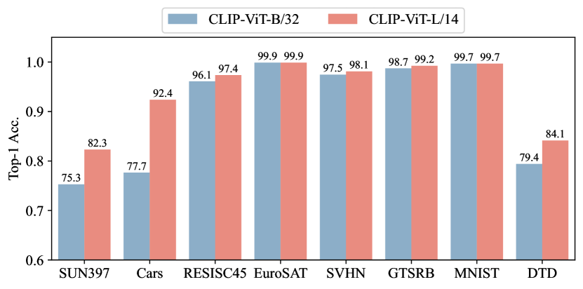
(a) Individual performance of fine-tuned CLIP-ViT-B/32 and CLIP-ViT-L/14 models.

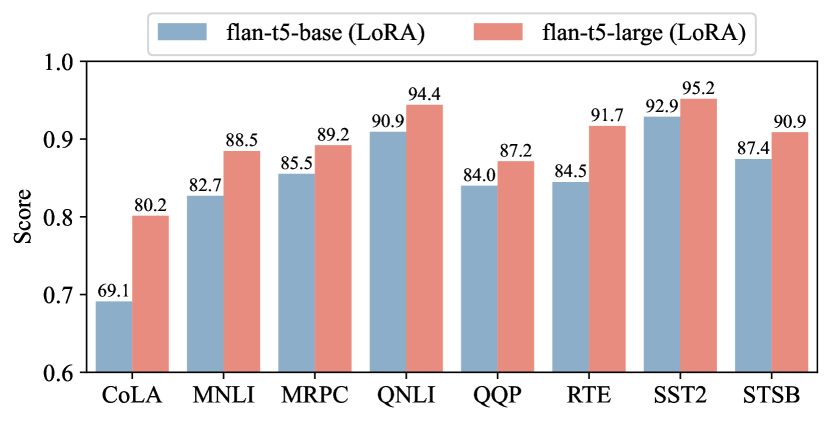
(b) Individual performance of LoRA fine-tuned flan-t5-base and flan-t5-large models.

Figure 4: Here we present a visual comparison of the performance of different fine-tuned models. The top figure compares the performance of the CLIP-ViT-B/32 and CLIP-ViT-L/14 models on image classification tasks, while the bottom figure compares the performance of the LoRA fine-tuned Flan-t5-base and Flan-t5-large models on tasks from GLUE benchmark.

Appendix C Multi-task Model Fusion Details

This section provides further implementation and configuration details for the baseline methods been compared in our experiments alongside a straightforward taxonomy of these methods. Subsequently, Appendix C.2 and Appendix C.3, serve to thoroughly explicate task arithmetic-based methods and AdaMerging-based methods. In these supplementary sections, we also provide a comprehensive analysis of the experimental results to afford clarity and facilitate a deeper understanding of the effectiveness of each multi-task strategy.

C.1 Details about Baseline Methods

• Simple Weight Average: We average the weights of the models fine-tuned on different tasks, this method is also referred to as ModelSoups [Wortsman et al., 2022] in the literature. The averaged model is then evaluated on the validation set of each task. For full fine-tuned models, the weights of the models are averaged directly (i.e., let $\theta={1/n\sum_{i=1}^{n}\theta_{i}}$). For LoRA fine-tuning, we average the weights of merged models, i.e., let $\theta=\theta_{0}+1/n\sum_{i}A_{i}B_{i}$.

• Task Arithmetic [Ilharco et al., 2023]: As defined in Section 3.1, the task vector is computed on the set of model parameters. We compute the task vector for each task and then add them to construct a multi-task vector. The multi-task vector is then multiplied by a scaling coefficient $\lambda$ element-wisely and added to the initial parameters of the pre-trained model to obtain a multi-task model, i.e. $\theta=\theta_{0}+\lambda\sum_{i}(\theta_{i}-\theta_{0})$ for full fine-tuning and $\phi=\phi_{0}+\lambda\sum_{i}A_{i}B_{i}$ for LoRA fine-tuning, where $\lambda$ is a hyperparameter that the best-performing model is chosen on validation set. In our study, $\lambda$ is chosen to be $0.3$.

• Ties-Merging [Yadav et al., 2023]: Ties-merging is a method for merging multiple task-specific models into a single multi-task model. This algorithm follows three steps (trim, elect sign of parameters, and disjoint merge) to obtain a merged task vector $\nu$. Given the final merged task vector $\tau$, the final model is chosen in a similar way as task arithmetic, i.e. $\theta=\theta_{0}+\lambda\tau$, where $\lambda$ is a hyperparameter that the best-performing model is chosen on the validation set. In our study, $\lambda$ is chosen to be $0.3$.

• AdaMerging [Yang et al., 2023]: AdaMerging is an adaptive model merging method where it autonomously autonomously learns the coefficients for merging either on a task-wise or layer-wise basis, using entropy minimization on unlabeled test samples as a surrogate objective function to refine the merging coefficients. The task-wise AdaMerging is formulated as $\theta=\theta_{0}+\sum_{i=1}^{n}\lambda_{i}\tau_{i}$ where $\lambda_{k}$ is the merging coefficient for the $k$-th task and $\tau_{k}$ is the task vector for the $k$-th task. The layer-wise AdaMerging is formulated as $\theta^{l}=\theta_{0}^{l}+\sum_{i=1}^{n}\lambda^{l}_{i}\tau^{l}_{i}$. In our study, we initialize the $\lambda$ to be $0.3$ for all tasks and layers.

A simple taxonomy of model merging methods. In this paper, we categorize the methods briefly into three groups: task arithmetic-based methods, AdaMerging-based methods, and others. Task arithmetic-based methods involve constructing a merged task vector, which is then scaled by a single factor and added to the pre-trained model. While AdaMerging-based methods assign separate task-wise or layer-wise weights to each task vector. In the following subsections, we will present some details about the experimental results of Task arithmetic-based methods and AdaMerging-based methods.

C.2 Task Arithmetic-Based Methods

The core procedure in task arithmetic-based methods includes the generation of a composite task vector. This composite task vector is an amalgamation of information relevant to each task, carefully constructed to preserve the distinctive features that define them. When this vector is ready, it goes through a scaling step. After being scaled, this adjusted task vector is merged right into the pre-trained model’s existing parameters. We describe this process mathematically as:

$$\theta=\theta_{0}+\lambda\mathcal{A}(\mathcal{T}),$$ (15)

where $\mathcal{A}:\mathbb{R}^{d\times n}\mapsto\mathbb{R}^{d}$ represents a merging algorithm for multiple tasks, $\mathcal{T}$ is a collection of task vectors $\{\tau_{i}\}_{i=1}^{n}$, and $d$ indicates the size of the model parameters. It’s akin to performing arithmetic on the knowledge of the model—adding new insights or amplifying existing ones.

One of the critical advantages of task arithmetic-based methods is the simplicity of the concept and its implementation. By leveraging a single scaling coefficient, the method offers a direct and computationally efficient way to transfer knowledge and adapt models to handle various tasks.

Despite their elegant simplicity, these methods require careful consideration in the determination of the scaling coefficient. The right balance ensures that the merged task vector harmoniously enhances the pre-trained model’s knowledge without overshadowing the valuable insights the model has already acquired. Balancing this interplay is crucial for the success of the task arithmetic approach.

Task arithmetic-based model merging thus stands out for its straightforwardness, ease of implementation, and potential to enable pre-trained models to excel across a wider array of tasks through a calculated, additive enhancement of their capabilities. In the following paragraphs, we will dive deeper into the experimental results garnered from employing these methods, offering a clear insight into their practical implications and the extent of their applicability.

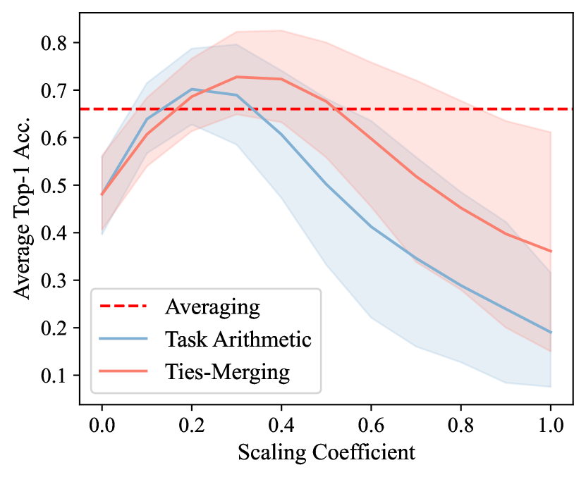
(a) CLIP-ViT-B/32

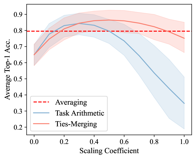
(b) CLIP-ViT-L/14

(c) Flan-T5-base (LoRA fine-tuned)

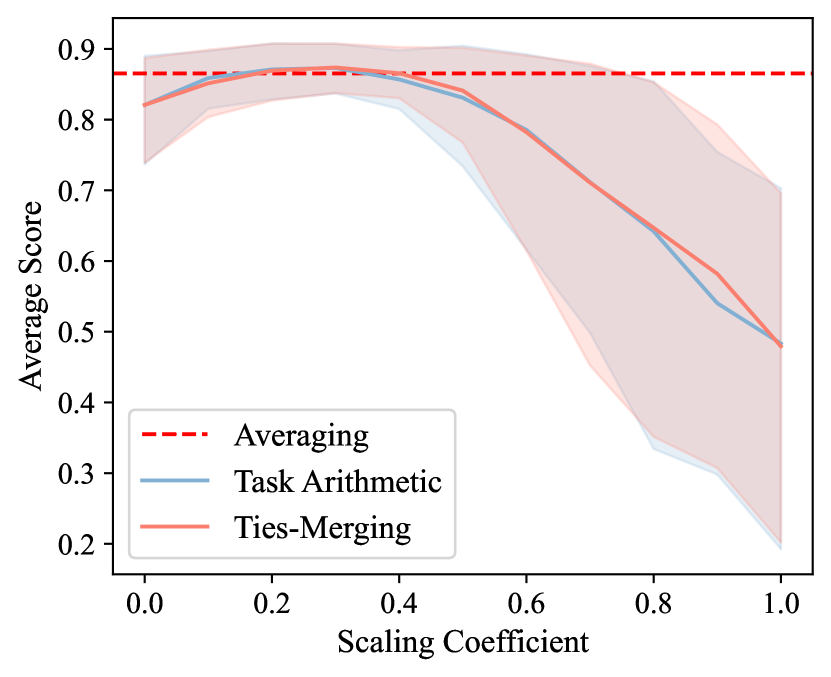
(d) Flan-T5-large (LoRA fine-tuned)

Figure 5: Task Arithmetic and Ties-Merging. Here we illustrate the average performance of models merged using Task Arithmetic and Ties-Merging methods, with varying scaling coefficients. The subfigures represent different models: CLIP-ViT-B/32, CLIP-ViT-L/14, Flan-T5-base (LoRA fine-tuned), and Flan-T5-large (LoRA fine-tuned).

In Figure 5, we show the average performance of Task Arithmetic and Ties-Merging merged models as the scaling coefficient varies. Figure 5(a), 5(b), 5(c), and 5(d) show the results of CLIP-ViT-B/32, CLIP-ViT-L/14, Flan-T5-base (LoRA fine-tuned), and Flan-T5-large (LoRA fine-tuned), respectively. It is evident that the merged multi-task model hits a peak in average performance across various tasks when the scaling coefficient is set around 0.3. This value was empirically selected as the scaling coefficient in our experiments. As we increase the scaling coefficient beyond this point, the average performance of the model begins to decline, eventually even falling below the level of the pre-trained model’s original performance. This suggests that too high of a scaling coefficient can have a negative impact on the knowledge that the pre-trained model initially possessed, emphasizing the importance of calibrating the scaling coefficient parameter $\lambda$ to avoid diminishing the model’s existing strengths.

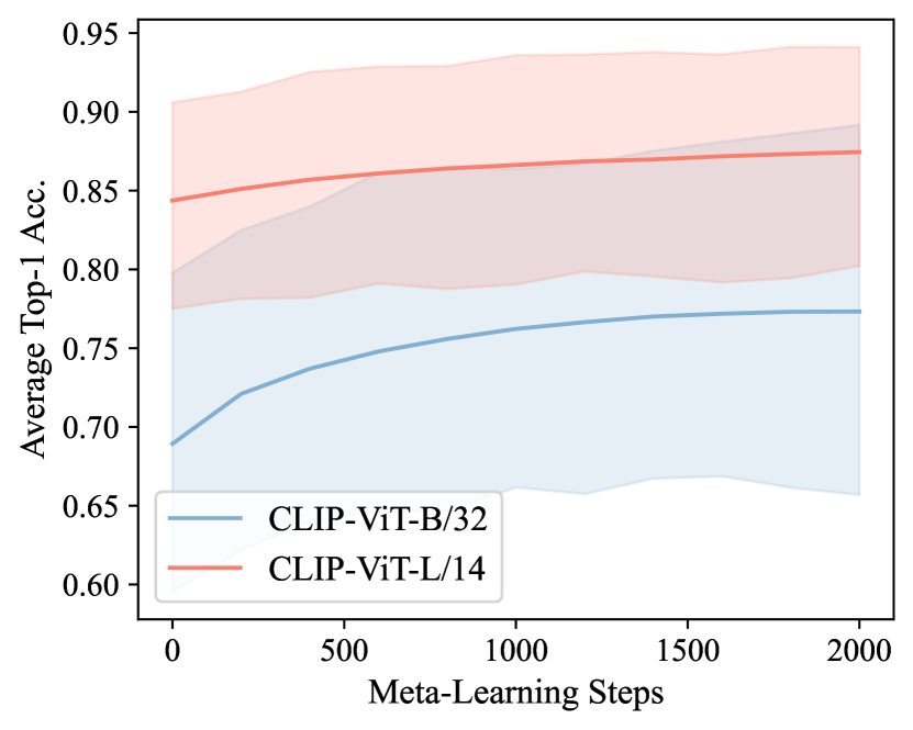
(a) CLIP models

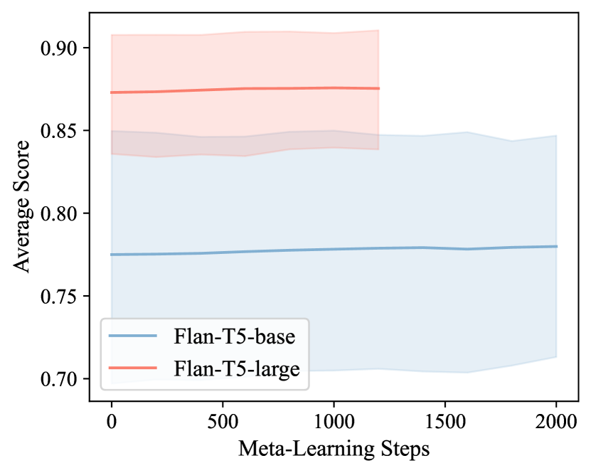
(b) Flan-T5 models

Figure 6: Concrete Task Arithmetic. The average performance of Concrete Task Arithmetic merged models as the learning step increases.

The pseudo-code for combining our Concrete Subspace Learning with task arithmetic is illustrated in Algorithm 2, namely Concrete Task Arithmetic. This algorithm outlines the steps involved in integrating our Concrete Subspace Learning approach with the task arithmetic method. Our procedure begins by employing Algorithm 1 to determine the Concrete mask. Throughout our experimental procedures, we have specifically set the scaling coefficient to 0.3 and have conducted the meta-learning process for 2000 steps. The learning rate is set to 1e-3 for CLIP models and 1e-4 for Flan-T5 models. Following this, we assess the performance of the model on the test dataset. The changes in the average model performance during the meta-learning phase of the Concrete task arithmetic are depicted in Figure 6 , where we observe a consistent and gradual improvement in model’s average performance.

Table 10: CLIP-ViT-B/32 with task arithmetic. We shows the performance of the merged model with different scaling coefficients on various datasets.

Scaling Coeff.	SUN397	Cars	RESISC45	EuroSAT	SVHN	GTSRB	MNIST	DTD	Avg.
0.0	63.2	59.6	60.2	45.0	31.6	32.6	48.2	44.4	48.1
0.1	65.0	63.0	70.3	71.2	59.4	48.6	83.8	49.9	63.9
0.2	63.8	62.1	72.0	78.1	74.4	65.1	94.0	52.2	70.2
0.3	55.3	54.9	66.7	77.4	80.2	69.7	97.3	50.1	69.0
0.4	36.7	41.0	53.8	66.4	80.6	66.0	98.1	42.5	60.7
0.5	18.2	23.2	38.7	53.9	77.8	57.4	97.8	34.5	50.2
0.6	8.0	9.5	25.1	45.8	73.0	45.5	96.2	27.0	41.3
0.7	3.5	2.8	16.7	39.9	67.1	35.0	91.9	20.2	34.6
0.8	1.4	1.2	11.4	34.7	60.0	25.2	83.3	14.0	28.9
0.9	0.7	0.9	8.4	31.1	52.7	17.7	69.6	10.4	24.0
1.0	0.4	0.7	6.7	27.7	44.6	15.2	49.4	7.8	19.1

Table 11: CLIP-ViT-B/32 with Ties-Merging. We shows the performance of the merged model with different scaling coefficients on various datasets.

Scaling Coeff.	SUN397	Cars	RESISC45	EuroSAT	SVHN	GTSRB	MNIST	DTD	Avg.
0.0	63.2	59.6	60.2	45.0	31.6	32.6	48.2	44.4	48.1
0.1	65.3	62.6	68.7	63.9	51.9	45.0	79.2	49.0	60.7
0.2	66.5	64.9	73.0	72.1	70.0	58.8	91.6	52.3	68.6
0.3	65.0	64.3	74.7	76.8	81.3	69.4	96.5	54.3	72.8
0.4	59.2	59.8	71.7	77.6	86.3	72.9	98.2	52.8	72.3
0.5	46.5	51.1	64.5	72.3	88.3	71.6	98.8	47.8	67.6
0.6	29.3	39.9	52.9	60.0	88.8	67.3	99.0	41.0	59.8
0.7	15.3	28.4	39.2	49.2	88.0	61.5	98.9	34.3	51.8
0.8	7.1	17.7	27.5	42.4	86.4	53.0	98.7	28.8	45.2
0.9	3.3	9.4	20.0	35.3	84.2	44.4	98.4	23.2	39.8
1.0	1.6	4.5	15.0	31.0	81.3	37.7	97.9	20.0	36.1

Table 12: CLIP-ViT-B/32 with Concrete Task Arithmetic. We show the performance of the merged model with increasing test-time adaptation steps on various datasets, see Algorithm 1 and 2. The performance of the merged model improves consistently as the number of test-time adaptation steps increases, which demonstrates the effectiveness of our Concrete Task Arithmetic to resolve task interference.

Step	SUN397	Cars	RESISC45	EuroSAT	SVHN	GTSRB	MNIST	DTD	Avg.
0	55.2	54.7	66.7	77.8	80.4	69.4	97.3	49.9	68.9
200	58.3	59.3	70.9	85.2	82.4	72.0	97.7	51.0	72.1
400	59.8	61.0	72.7	88.9	84.4	73.2	98.0	51.7	73.7
600	60.3	61.4	73.9	91.4	85.8	75.3	98.1	51.9	74.8
800	61.2	62.5	74.3	92.9	87.0	76.8	98.2	51.8	75.6
1000	61.6	62.2	74.9	94.1	87.9	78.5	98.2	52.3	76.2
1200	61.8	62.2	75.2	94.7	89.0	79.8	98.4	52.1	76.6
1400	62.2	62.1	75.3	95.0	89.5	81.1	98.4	51.9	77.0
1600	62.4	61.6	75.7	95.4	90.2	81.4	98.5	52.2	77.2
1800	62.6	61.8	76.0	95.4	90.6	81.7	98.5	51.9	77.3
2000	62.5	61.1	76.0	95.7	91.0	81.9	98.5	51.9	77.3

Table 10, 11 and Table 12 show the performance of CLIP-ViT-B/32 with task arithmetic, Ties-Merging, and Concrete Task Arithmetic, respectively. Each table shows how performance varies across a set of benchmark datasets with different scaling coefficients or adaptation steps.

For both Task Arithmetic and Tie-Merging, we observed an initial increase in performance across most tasks as the scaling coefficient increased. The peak performance was typically achieved around a scaling coefficient of 0.3, after which the performance began to decline rapidly on most tasks. This decline can be attributed to the competition and interference among various tasks. As the scaling coefficient increases, the model tends to overfit certain tasks, leading to a decrease in performance on other tasks. This phenomenon was particularly noticeable on the SVHN and MNIST datasets.

In contrast, for Concrete Task Arithmetic, we noticed a gradual improvement in model performance with an increase in the number of adaptation steps. These results indicate that performing model merging under the common subspace learned through meta-learning can help resolve interference among downstream tasks.

C.3 AdaMerging-Based Methods

AdaMerging-based methods form a distinct category within the landscape of model merging strategies, where the primary focus is on refinement. Unlike task arithmetic-based methods that rely on a uniform scaling coefficient, AdaMerging-based strategies introduce a fine-grained approach by assigning unique weights to each task or different layers within the task vector. This nuanced weighting mechanism allows for a more personalized integration of task-specific knowledge into the pre-trained model. We describe this process mathematically as:

$$\theta=\theta_{0}+\sum_{i=1}^{n}\lambda_{i}\mathcal{A}(\tau_{i})\quad\text{or}\quad\theta^{l}=\theta_{0}^{l}+\sum_{i=1}^{n}\lambda^{l}_{i}\mathcal{A}(\tau^{l}_{i}).$$ (16)

Here, $\mathcal{A}$ represents a transformation applied to the task vector $\tau_{i}$, such as masking and rescaling in our Concrete AdaMerging (Algorithm 3), as well as the elimination of redundant parameter values and resolution of sign conflicts in AdaMerging++ [Yang et al., 2023].

Fundamentally, AdaMerging recognizes the diversity of tasks and their varying degrees of relevance to the underlying model. This can be particularly advantageous when dealing with tasks of varying complexity or dissimilar data distributions. For layers, the approach allows the model to capitalize on the hierarchical representation of features at different levels of abstraction. In practice, this translates into a meticulous process of weight allocation that considers the specific contribution of each task, or the particular influence of each layer when merging with a pre-trained model’s existing knowledge base by performing test-time adaptation on unlabeled test samples.

The versatility of AdaMerging-based methods lends itself well to complex multi-task learning scenarios. It has the potential to finely balance task-specific learning without risking the dilution of the model’s core competencies. Moreover, by treating different tasks and layers with individual consideration, AdaMerging-based methods can effectively restrain the negative interference often witnessed when a model is adjusted to new tasks that are substantially different from the ones it was originally trained on.

In the upcoming paragraphs, we will explore the experimental results obtained from the utilization of AdaMerging and our Concrete AdaMerging. This exploration aims to offer a detailed understanding of their practical implications and the extent of their applicability.

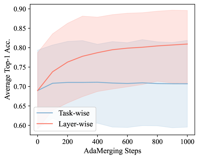
(a) CLIP-ViT-B/32

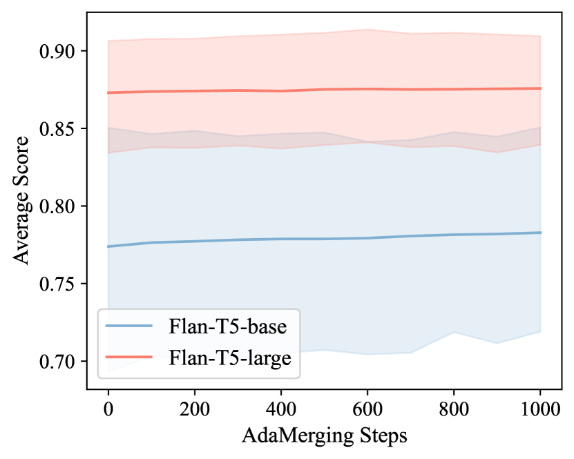
(b) Flan-T5 models with layer-wise AdaMerging

Figure 7: AdaMerging. The average performance of AdaMerging merged models as the learning step increases.

Figure 7 shows the average performance of AdaMerging merged models as the learning step increases. Specifically, Figure 7(a) shows the results of CLIP-ViT-B/32 with both task-wise AdaMerging and layer-wise AdaMerging, and Figure 7(b) shows the results of Flan-T5-base and Flan-T5-large models with layer-wise AdaMerging.

We observe that the average performance of the model increases as the learning step increases. This suggests that the AdaMerging merged model can benefit from the test-time adaptation process and improve its performance on the test dataset. In the case of CLIP-ViT-B/32, the average performance of the model with layer-wise AdaMerging is higher than the model with task-wise AdaMerging. This is because the layer-wise AdaMerging allows the model to adapt to different tasks at different layers, which is more flexible than the task-wise AdaMerging. In the case of Flan-T5-base and Flan-T5-large, the average performance of Flan-T5-large is higher than Flan-T5-base, which indicates that the model with more parameters can benefit more from the AdaMerging.

As for our Concrete AdaMerging, as explained in Algorithm 3, we first use Algorithm 1 to determine the Concrete mask. Then, we use the Concrete mask to mask the task vector and rescale it to obtain the final task vector to perform normal AdaMerging. We conduct the meta-learning process for 2000 steps and the AdaMerging process for 1000 steps. We use Adam optimizer to optimize the parameters. The learning rate settings are $\alpha=1,\beta=0.001$ for CLIP models and $\alpha=0.1,\beta=0.0001$ for Flan-T5 models. During the test-time adaptation phase, we set the learning rate to $\beta$.

(a) Meta-learn the Concrete mask

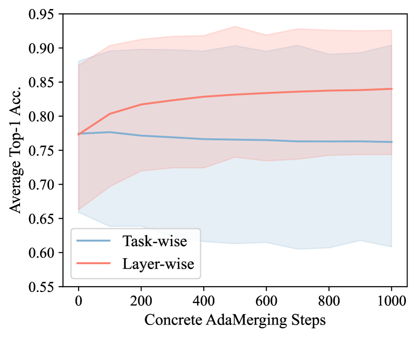
(b) AdaMerging with the Concrete mask

Figure 8: CLIP-ViT-B/32 with Concrete AdaMerging. Here we show the whole process of applying Concrete AdaMerging to CLIP-ViT-B/32, the y-axis is shared by these two subfigures: (a) shows the performance of the merged model during the meta-learning phase of the Concrete AdaMerging, see Algorithm 1; (b) shows the performance of the model during the test-time adaptation phase of the Concrete AdaMerging, see Algorithm 3.

Figure 8 shows the whole process of applying Concrete AdaMerging to CLIP-ViT-B/32. Specifically, Figure 8(a) shows the changes in the average model performance during the meta-learning phase of the Concrete AdaMerging. We observe a consistent and gradual improvement in the model’s average performance. Figure 8(b) shows the changes in the average model performance during the test-time adaptation phase of the Concrete AdaMerging. We observe that the average performance of the model increases as the learning step increases, which indicates that Concrete AdaMerging can benefit from the test-time adaptation process and improve its performance on the test dataset.

Table 13: CLIP-ViT-B/32 with Layer-wise AdaMerging. We show the performance of the merged model with increasing test-time adaptation steps on various datasets.

TTA Step	SUN397	Cars	RESISC45	EuroSAT	SVHN	GTSRB	MNIST	DTD	Avg
0	55.3	54.9	66.7	77.4	80.2	69.7	97.3	50.1	69
100	59.7	60.4	72.2	88.3	84.4	76.7	97.6	51.0	73.8
200	61.4	63.6	74.4	92.0	85.6	83.5	97.5	52.4	76.3
300	62.3	65.4	75.9	92.4	86.5	87.9	97.5	54.4	77.8
400	63.1	66.7	77.7	92.5	86.2	90.5	97.1	55.8	78.7
500	63.6	67.5	79.3	92.4	86.6	91.9	97.3	57.3	79.5
600	64.0	68.1	79.5	92.4	86.6	92.8	97.2	58.5	79.9
700	64.1	68.5	80.0	92.4	86.5	92.9	97.4	59.0	80.1
800	64.0	69.1	81.5	92.5	86.3	93.3	97.4	59.6	80.5
900	64.1	69.3	82.3	92.7	86.0	93.6	97.5	60.2	80.7
1000	64.2	69.5	82.4	92.5	86.5	93.7	97.6	61.1	80.9

Table 14: CLIP-ViT-B/32 with Layer-wise Concrete AdaMerging. We show the performance of the merged model with increasing test-time adaptation steps on various datasets.

TTA Step	SUN397	Cars	RESISC45	EuroSAT	SVHN	GTSRB	MNIST	DTD	Avg
0	62.2	62.8	77.2	92.9	85.8	84.3	98.3	55.0	77.3
100	63.9	65.6	81.2	94.9	89.3	91.4	98.6	57.9	80.3
200	64.9	67.3	83.7	95.7	89.9	94.0	98.5	59.7	81.7
300	65.2	67.9	84.9	95.6	90.1	95.2	98.5	61.2	82.3
400	66.0	68.4	85.7	95.9	90.6	95.7	98.6	62.0	82.9
500	66.4	68.7	86.2	95.7	91.2	96.1	98.6	62.5	83.2
600	66.7	68.9	86.5	95.8	91.4	96.2	98.6	63.1	83.4
700	66.9	69.3	86.8	95.8	91.6	96.3	98.7	63.4	83.6
800	67.4	69.5	87.0	95.8	91.6	96.4	98.7	63.6	83.8
900	67.5	69.7	87.1	95.9	91.4	96.6	98.7	63.7	83.8
1000	67.8	70.0	87.5	96.0	91.6	96.7	98.7	63.8	84.0

In Table 13 and Table 14, we show the performance of merged CLIP-ViT-B/32 across various downstream tasks with layer-wise AdaMerging and layer-wise Concrete AdaMerging, respectively. We observed that the performance of both Layer-wise AdaMerging and Layer-wise Concrete AdaMerging on various downstream tasks consistently improved with the progression of test-time adaptation. Notably, given the same number of update steps, Layer-wise Concrete AdaMerging generally outperformed Layer-wise AdaMerging. This suggests that performing model fusion on the common subspace learned during meta-training can effectively resolve the interference among tasks. These findings validate the effectiveness of our proposed method. Furthermore, they highlight the potential of leveraging learned common subspaces for model fusion, especially in scenarios where task interference could pose a significant challenge.

Appendix D Implementation Details

In this section, we provide more details about the implementation of our method.

D.1 Preprocessed Examples of GLUE Benchmark

Flan-T5 models embody the encoder-decoder architecture specific to transformer models, operating within a text-to-text framework. So we reformat the initial inputs into a structure that aligns with this text-to-text paradigm. In this subsection, we will present a range of instances demonstrating how the data has been preprocessed to fit the requirements of the GLUE (General Language Understanding Evaluation) benchmarks [Wang et al., 2018].

We report exact match accuracy for all tasks except for STSB, where we report Spearman’s $\rho$.

D.1.1 CoLA

We assign label 0 as “unacceptable” and label 1 as “acceptable”.

Original inputs:

• sentence: Our friends won’t buy this analysis, let alone the next one we propose.

• label: 1

Preprocessed:

• input: Indicate if the following sentence is grammatically correct or not: “Our friends won’t buy this analysis, let alone the next one we propose.”. Answere ‘acceptable’ or ‘unacceptable’.

• target: acceptable

D.1.2 MNLI

We assign label 0 as “entailment”, label 1 as “neutral” and label 2 as “contradiction”.

Original inputs:

• hypothesis: Product and geography are what make cream skimming work.

• premise: Conceptually cream skimming has two basic dimensions - product and geography.

• label: 1

Preprocessed:

• input: Does the premise: ‘Product and geography are what make cream skimming work.’ logically imply, contradict, or is neutral to the hypothesis: ‘Conceptually cream skimming has two basic dimensions - product and geography.’? Answere with ‘entailment’, ‘contradiction’, or ‘neutral’.

• target: neutral

D.1.3 MRPC

We assign label 0 as “no” and label 1 as “yes”.

Original inputs:

• sentence1: Amrozi accused his brother, whom he called “the witness”, of deliberately distorting his evidence.

• sentence2: Referring to him as only “the witness”, Amrozi accused his brother of deliberately distorting his evidence.

• label: 1

Preprocessed:

• input: Are the following sentences ‘Amrozi accused his brother, whom he called “the witness”, of deliberately distorting his evidence.’ and ‘Referring to him as only “the witness”, Amrozi accused his brother of deliberately distorting his evidence.’ conveying the same meaning? Answere with ‘yes’ or ‘no’.

• target: yes

D.1.4 QNLI

we assign label 0 as “yes” and label 1 as “no”.

Original inputs:

• question: What kind of test does the doctor perform?

• sentence: The doctor performs a test to see if you have strep throat.

• label: 1

Preprocessed:

• input: Given the context: ‘The doctor performs a test to see if you have strep throat.’, does the question ‘What kind of test does the doctor perform?’ have an answer based on the information provided? Answer with ‘yes’ or ‘no’.

• target: yes

D.1.5 QQP

We assign label 0 as “no” and label 1 as “yes”.

Original inputs:

• question1: How is the life of a math student? Could you describe your own experiences?

• question2: Which level of prepration is enough for the exam jlpt5?

• label: 0

Preprocessed:

• input: Do the questions ‘How is the life of a math student? Could you describe your own experiences?’ and ‘Which level of prepration is enough for the exam jlpt5?’ have the same intent? Answere with ‘yes’ or ‘no’.

• target: no

D.1.6 RTE

We assign label 0 as “yes” and label 1 as “no”.

Original inputs:

• sentence1: No Weapons of Mass Destruction Found in Iraq Yet.

• sentence2: Weapons of Mass Destruction Found in Iraq.

• label: 1

Preprocessed:

• input: Does the text: ‘No Weapons of Mass Destruction Found in Iraq Yet.’ entail that ‘Weapons of Mass Destruction Found in Iraq.’ is true? Provide ‘yes’ or ‘no’.

• target: no

D.1.7 SST2

We assign label 0 as “negative” and label 1 as “positive”.

Original inputs:

• sentence: hide new secretions from the parental units

• label: 0

Preprocessed:

• input: Given the sentence ‘hide new secretions from the parental units’, determine the sentiment. Is it positive or negative?

• target: negative

D.1.8 STSB

We format the ‘label’ argument as a string with one decimal place, the corresponding Python code is ‘"{:.1f}".format(label)‘.

Original inputs:

• sentence1: A plane is taking off.

• sentence2: An air plane is taking off.

• label: 5

Preprocessed:

• input: Consider the sentences ‘A plane is taking off.’ and ‘An air plane is taking off.’. On a scale from 1 (completely different) to 5 (completely similar), rate the similarity.

• target: 5.0

References

- He et al. [2016] Kaiming He, Xiangyu Zhang, Shaoqing Ren, and Jian Sun. Deep residual learning for image recognition. Proceedings of the IEEE Computer Society Conference on Computer Vision and Pattern Recognition, 2016-Decem:770–778, 2016. ISSN 10636919. doi:10.1109/CVPR.2016.90.
- He et al. [2021] Kaiming He, Xinlei Chen, Saining Xie, Yanghao Li, Piotr Dollár, and Ross Girshick. Masked Autoencoders Are Scalable Vision Learners, December 2021. URL http://arxiv.org/abs/2111.06377.
- Radford et al. [2019] Alec Radford, Jeffrey Wu, Rewon Child, David Luan, Dario Amodei, and Ilya Sutskever. Language Models are Unsupervised Multitask Learners. 1:9, 2019.
- Chung et al. [2022] Hyung Won Chung, Le Hou, Shayne Longpre, Barret Zoph, Yi Tay, William Fedus, Yunxuan Li, Xuezhi Wang, Mostafa Dehghani, Siddhartha Brahma, Albert Webson, Shixiang Shane Gu, Zhuyun Dai, Mirac Suzgun, Xinyun Chen, Aakanksha Chowdhery, Alex Castro-Ros, Marie Pellat, Kevin Robinson, Dasha Valter, Sharan Narang, Gaurav Mishra, Adams Yu, Vincent Zhao, Yanping Huang, Andrew Dai, Hongkun Yu, Slav Petrov, Ed H. Chi, Jeff Dean, Jacob Devlin, Adam Roberts, Denny Zhou, Quoc V. Le, and Jason Wei. Scaling Instruction-Finetuned Language Models, December 2022. URL http://arxiv.org/abs/2210.11416.
- Gulati et al. [2020] Anmol Gulati, James Qin, Chung-Cheng Chiu, Niki Parmar, Yu Zhang, Jiahui Yu, Wei Han, Shibo Wang, Zhengdong Zhang, Yonghui Wu, and Ruoming Pang. Conformer: Convolution-augmented Transformer for Speech Recognition, May 2020. URL http://arxiv.org/abs/2005.08100.
- Li et al. [2023] Weishi Li, Yong Peng, Miao Zhang, Liang Ding, Han Hu, and Li Shen. Deep Model Fusion: A Survey, September 2023. URL http://arxiv.org/abs/2309.15698.
- Zheng et al. [2023] Hongling Zheng, Li Shen, Anke Tang, Yong Luo, Han Hu, Bo Du, and Dacheng Tao. Learn From Model Beyond Fine-Tuning: A Survey, October 2023. URL http://arxiv.org/abs/2310.08184.
- Wu et al. [2019] Xi Zhu Wu, Song Liu, and Zhi Hua Zhou. Heterogeneous model reuse via optimizing multiparty multiclass margin. 36th International Conference on Machine Learning, ICML 2019, 2019-June:11862–11871, 2019.
- Tang et al. [2023a] Anke Tang, Yong Luo, Han Hu, Fengxiang He, Kehua Su, Bo Du, Yixin Chen, and Dacheng Tao. Improving Heterogeneous Model Reuse by Density Estimation. In Thirty-Second International Joint Conference on Artificial Intelligence, volume 4, pages 4244–4252, August 2023a. doi:10.24963/ijcai.2023/472. URL https://www.ijcai.org/proceedings/2023/472.
- Ilharco et al. [2023] Gabriel Ilharco, Marco Tulio Ribeiro, Mitchell Wortsman, Suchin Gururangan, Ludwig Schmidt, Hannaneh Hajishirzi, and Ali Farhadi. Editing Models with Task Arithmetic, March 2023. URL http://arxiv.org/abs/2212.04089.
- Yadav et al. [2023] Prateek Yadav, Derek Tam, Leshem Choshen, Colin Raffel, and Mohit Bansal. Resolving Interference When Merging Models, June 2023. URL http://arxiv.org/abs/2306.01708.
- Yu et al. [2023] Le Yu, Bowen Yu, Haiyang Yu, Fei Huang, and Yongbin Li. Language Models are Super Mario: Absorbing Abilities from Homologous Models as a Free Lunch, November 2023. URL http://arxiv.org/abs/2311.03099.
- Daniel Freeman and Bruna [2017] C. Daniel Freeman and Joan Bruna. Topology and geometry of half-rectified network optimization: 5th International Conference on Learning Representations, ICLR 2017. 2017. URL http://www.scopus.com/inward/record.url?scp=85064823226&partnerID=8YFLogxK.
- Nagarajan and Kolter [2019] Vaishnavh Nagarajan and J. Zico Kolter. Uniform convergence may be unable to explain generalization in deep learning. In Advances in Neural Information Processing Systems, volume 32. Curran Associates, Inc., 2019. URL https://proceedings.neurips.cc/paper_files/paper/2019/hash/05e97c207235d63ceb1db43c60db7bbb-Abstract.html.
- Draxler et al. [2019] Felix Draxler, Kambis Veschgini, Manfred Salmhofer, and Fred A. Hamprecht. Essentially No Barriers in Neural Network Energy Landscape, February 2019. URL http://arxiv.org/abs/1803.00885.
- Entezari et al. [2022] Rahim Entezari, Hanie Sedghi, Olga Saukh, and Behnam Neyshabur. The Role of Permutation Invariance in Linear Mode Connectivity of Neural Networks, July 2022. URL http://arxiv.org/abs/2110.06296.
- Garipov et al. [2018] Timur Garipov, Pavel Izmailov, Dmitrii Podoprikhin, Dmitry Vetrov, and Andrew Gordon Wilson. Loss Surfaces, Mode Connectivity, and Fast Ensembling of DNNs, October 2018. URL http://arxiv.org/abs/1802.10026.
- Tatro et al. [2020] Norman Tatro, Pin-Yu Chen, Payel Das, Igor Melnyk, Prasanna Sattigeri, and Rongjie Lai. Optimizing Mode Connectivity via Neuron Alignment. In Advances in Neural Information Processing Systems, volume 33, pages 15300–15311. Curran Associates, Inc., 2020. URL https://proceedings.neurips.cc/paper/2020/hash/aecad42329922dfc97eee948606e1f8e-Abstract.html.
- Yunis et al. [2022] David Yunis, Kumar Kshitij Patel, Pedro Savarese, Gal Vardi, Karen Livescu, Matthew Walter, Jonathan Frankle, and Michael Maire. On Convexity and Linear Mode Connectivity in Neural Networks. OPT2022: 14th Annual Workshop on Optimization for Machine Learning, 2022.
- Matena and Raffel [2022] Michael Matena and Colin Raffel. Merging Models with Fisher-Weighted Averaging, August 2022. URL http://arxiv.org/abs/2111.09832.
- Wortsman et al. [2022] Mitchell Wortsman, Gabriel Ilharco, Samir Yitzhak Gadre, Rebecca Roelofs, Raphael Gontijo-Lopes, Ari S. Morcos, Hongseok Namkoong, Ali Farhadi, Yair Carmon, Simon Kornblith, and Ludwig Schmidt. Model soups: Averaging weights of multiple fine-tuned models improves accuracy without increasing inference time, July 2022. URL http://arxiv.org/abs/2203.05482.
- Kaddour [2022] Jean Kaddour. Stop Wasting My Time! Saving Days of ImageNet and BERT Training with Latest Weight Averaging, October 2022. URL http://arxiv.org/abs/2209.14981.
- Izmailov et al. [2019] Pavel Izmailov, Dmitrii Podoprikhin, Timur Garipov, Dmitry Vetrov, and Andrew Gordon Wilson. Averaging Weights Leads to Wider Optima and Better Generalization, February 2019. URL http://arxiv.org/abs/1803.05407.
- Li et al. [2016] Yixuan Li, Jason Yosinski, Jeff Clune, Hod Lipson, and John Hopcroft. Convergent Learning: Do different neural networks learn the same representations?, February 2016. URL http://arxiv.org/abs/1511.07543.
- George Stoica et al. [2023] George Stoica, Daniel Bolya, Jakob Bjorner, Taylor Hearn, and Judy Hoffman. ZipIt! Merging Models from Different Tasks without Training, May 2023. URL http://arxiv.org/abs/2305.03053.
- Jin et al. [2023] Xisen Jin, Xiang Ren, Daniel Preotiuc-Pietro, and Pengxiang Cheng. Dataless Knowledge Fusion by Merging Weights of Language Models, April 2023. URL http://arxiv.org/abs/2212.09849.
- Ainsworth et al. [2023] Samuel K. Ainsworth, Jonathan Hayase, and Siddhartha Srinivasa. Git Re-Basin: Merging Models modulo Permutation Symmetries, March 2023. URL http://arxiv.org/abs/2209.04836.
- Chronopoulou et al. [2023] Alexandra Chronopoulou, Matthew E. Peters, Alexander Fraser, and Jesse Dodge. AdapterSoup: Weight Averaging to Improve Generalization of Pretrained Language Models, March 2023. URL http://arxiv.org/abs/2302.07027.
- Huang et al. [2023] Chengsong Huang, Qian Liu, Bill Yuchen Lin, Tianyu Pang, Chao Du, and Min Lin. LoraHub: Efficient Cross-Task Generalization via Dynamic LoRA Composition, July 2023. URL http://arxiv.org/abs/2307.13269.
- Zhang et al. [2023] Jinghan Zhang, Shiqi Chen, Junteng Liu, and Junxian He. Composing Parameter-Efficient Modules with Arithmetic Operations, June 2023. URL http://arxiv.org/abs/2306.14870.
- Wu et al. [2023] Chengyue Wu, Teng Wang, Yixiao Ge, Zeyu Lu, Ruisong Zhou, Ying Shan, and Ping Luo. -Tuning: Transferring Multimodal Foundation Models with Optimal Multi-task Interpolation, May 2023. URL http://arxiv.org/abs/2304.14381.
- Tang et al. [2023b] Anke Tang, Li Shen, Yong Luo, Yibing Zhan, Han Hu, Bo Du, Yixin Chen, and Dacheng Tao. Parameter Efficient Multi-task Model Fusion with Partial Linearization, October 2023b. URL http://arxiv.org/abs/2310.04742.
- Yang et al. [2023] Enneng Yang, Zhenyi Wang, Li Shen, Shiwei Liu, Guibing Guo, Xingwei Wang, and Dacheng Tao. AdaMerging: Adaptive Model Merging for Multi-Task Learning, October 2023. URL http://arxiv.org/abs/2310.02575.
- Maddison et al. [2017] Chris J. Maddison, Andriy Mnih, and Yee Whye Teh. The Concrete Distribution: A Continuous Relaxation of Discrete Random Variables, March 2017. URL http://arxiv.org/abs/1611.00712.
- Jang et al. [2017] Eric Jang, Shixiang Gu, and Ben Poole. Categorical Reparameterization with Gumbel-Softmax, August 2017. URL http://arxiv.org/abs/1611.01144.
- Mounsaveng et al. [2023] Saypraseuth Mounsaveng, Florent Chiaroni, Malik Boudiaf, Marco Pedersoli, and Ismail Ben Ayed. Bag of Tricks for Fully Test-Time Adaptation, October 2023. URL http://arxiv.org/abs/2310.02416.
- Liang et al. [2023] Jian Liang, Ran He, and Tieniu Tan. A Comprehensive Survey on Test-Time Adaptation under Distribution Shifts, March 2023. URL http://arxiv.org/abs/2303.15361.
- Radford et al. [2021a] Alec Radford, Jong Wook Kim, Chris Hallacy, Aditya Ramesh, Gabriel Goh, Sandhini Agarwal, Girish Sastry, Amanda Askell, Pamela Mishkin, Jack Clark, Gretchen Krueger, and Ilya Sutskever. Learning Transferable Visual Models From Natural Language Supervision, February 2021a. URL http://arxiv.org/abs/2103.00020. arXiv:2103.00020 [cs].
- Xiao et al. [2010] Jianxiong Xiao, James Hays, Krista A. Ehinger, Aude Oliva, and Antonio Torralba. SUN database: Large-scale scene recognition from abbey to zoo. In 2010 IEEE Computer Society Conference on Computer Vision and Pattern Recognition, pages 3485–3492, San Francisco, CA, USA, June 2010. IEEE. ISBN 978-1-4244-6984-0. doi:10.1109/CVPR.2010.5539970. URL http://ieeexplore.ieee.org/document/5539970/.
- Krause et al. [2013] Jonathan Krause, Michael Stark, Jia Deng, and Li Fei-Fei. 3D Object Representations for Fine-Grained Categorization. In 2013 IEEE International Conference on Computer Vision Workshops, pages 554–561, December 2013. doi:10.1109/ICCVW.2013.77. URL https://ieeexplore.ieee.org/document/6755945.
- Cheng et al. [2017] Gong Cheng, Junwei Han, and Xiaoqiang Lu. Remote Sensing Image Scene Classification: Benchmark and State of the Art. Proceedings of the IEEE, 105(10):1865–1883, October 2017. ISSN 0018-9219, 1558-2256. doi:10.1109/JPROC.2017.2675998. URL http://arxiv.org/abs/1703.00121. arXiv:1703.00121 [cs].
- Helber et al. [2018] Patrick Helber, Benjamin Bischke, Andreas Dengel, and Damian Borth. Introducing eurosat: A novel dataset and deep learning benchmark for land use and land cover classification. In IGARSS 2018-2018 IEEE International Geoscience and Remote Sensing Symposium, pages 204–207. IEEE, 2018.
- Netzer et al. [2021] Yuval Netzer, Tao Wang, Adam Coates, Alessandro Bissacco, Bo Wu, and Andrew Y Ng. Reading Digits in Natural Images with Unsupervised Feature Learning. 2021.
- Stallkamp et al. [2012] J. Stallkamp, M. Schlipsing, J. Salmen, and C. Igel. Man vs. computer: Benchmarking machine learning algorithms for traffic sign recognition. Neural Networks, 32:323–332, August 2012. ISSN 0893-6080. doi:10.1016/j.neunet.2012.02.016. URL https://www.sciencedirect.com/science/article/pii/S0893608012000457.
- Lecun et al. [1998] Yann Lecun, Le’on Bottou, Yoshua Bengio, and Parick Haffner. Gradient-based learning applied to document recognition. Proceedings of the IEEE, 86(11):2278–2324, 1998. ISSN 00189219. doi:10.1109/5.726791. URL http://ieeexplore.ieee.org/document/726791/.
- Cimpoi et al. [2014] Mircea Cimpoi, Subhransu Maji, Iasonas Kokkinos, Sammy Mohamed, and Andrea Vedaldi. Describing Textures in the Wild. In 2014 IEEE Conference on Computer Vision and Pattern Recognition, pages 3606–3613, Columbus, OH, USA, June 2014. IEEE. ISBN 978-1-4799-5118-5. doi:10.1109/CVPR.2014.461. URL https://ieeexplore.ieee.org/document/6909856.
- Wang et al. [2018] Alex Wang, Amanpreet Singh, Julian Michael, Felix Hill, Omer Levy, and Samuel Bowman. GLUE: A Multi-Task Benchmark and Analysis Platform for Natural Language Understanding. In Proceedings of the 2018 EMNLP Workshop BlackboxNLP: Analyzing and Interpreting Neural Networks for NLP, pages 353–355, Brussels, Belgium, 2018. Association for Computational Linguistics. doi:10.18653/v1/W18-5446. URL http://aclweb.org/anthology/W18-5446.
- Gumbel [1954] E. J. Gumbel. Statistical Theory of Extreme Values and Some Practical Applications. A Series of Lectures. Technical Report PB175818, National Bureau of Standards, Washington, D. C. Applied Mathematics Div., 1954. URL https://ntrl.ntis.gov/NTRL/dashboard/searchResults/titleDetail/PB175818.xhtml.
- Luce [1959] R. Duncan Luce. Individual Choice Behavior. Individual Choice Behavior. John Wiley, Oxford, England, 1959.
- Maddison et al. [2014] Chris J Maddison, Daniel Tarlow, and Tom Minka. A* sampling. Advances in neural information processing systems, 27, 2014.
- Radford et al. [2021b] Alec Radford, Jong Wook Kim, Chris Hallacy, Aditya Ramesh, Gabriel Goh, Sandhini Agarwal, Girish Sastry, Amanda Askell, Pamela Mishkin, Jack Clark, Gretchen Krueger, and Ilya Sutskever. Learning Transferable Visual Models From Natural Language Supervision, February 2021b. URL http://arxiv.org/abs/2103.00020.
- Hu et al. [2021] Edward J. Hu, Yelong Shen, Phillip Wallis, Zeyuan Allen-Zhu, Yuanzhi Li, Shean Wang, Lu Wang, and Weizhu Chen. LoRA: Low-Rank Adaptation of Large Language Models, October 2021. URL http://arxiv.org/abs/2106.09685.