Adaptive Feature Selection for No-Reference Image Quality Assessment using Contrastive Mitigating Semantic Noise Sensitivity

Abstract

The current state-of-the-art No-Reference Image Quality Assessment (NR-IQA) methods typically use feature extraction in upstream backbone networks, which assumes that all extracted features are relevant. However, we argue that not all features are beneficial, and some may even be harmful, necessitating careful selection. Empirically, we find that many image pairs with small feature spatial distances can have vastly different quality scores. To address this issue, we propose a Quality-Aware Feature Matching IQA metric (QFM-IQM) that employs contrastive learning to remove harmful features from the upstream task. Specifically, our approach enhances the semantic noise distinguish capabilities of neural networks by comparing image pairs with similar semantic features but varying quality scores and adaptively adjusting the upstream task’s features by introducing disturbance. Furthermore, we utilize a distillation framework to expand the dataset and improve the model’s generalization ability. Our approach achieves superior performance to the state-of-the-art NR-IQA methods on 8 standard NR-IQA datasets, achieving PLCC values of 0.932 ($\uparrow 2.4\%$ vs. 0.908 in TID2013) and 0.913 ($\uparrow 1.9\%$ vs. 0.894 in LIVEC).

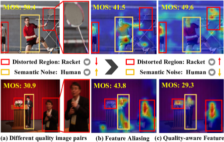
Figure 1: Images in the first column: the sample images in the KonIQ dataset. Images in the medium column: Quality attention map from DEIQT [31] which suffers from feature aliasing that focuses excessively on semantic-level noise that is less relevant to quality perception (e.g., the human in the yellow box). Images in the last column: Quality attention map from QFM-IQM. Our QFM-IQAM is not sensitive to semantic noise and can clearly distinguish between image pairs with similar semantic content but different quality scores. As a result, our model’s predictions are more aligned with the actual Mean Opinion Scores (MOS).

1 Introduction

No-Reference Image Quality Assessment (NR-IQA) is a fundamental research area [26, 6, 12, 45], which simulates the human subjective system to estimate distortion of the given image. Current state-of-the-art methods generally leverage pre-trained upstream backbone to extract semantic features, and then, finetuning on NR-IQA datasets. This pipeline provides an effective and efficient training procedure while reducing the requirement of data volume. since the semantic features obtained from the pre-trained upstream backbone have no direct correlation with the image quality representation, many researchers focus on the optimization of semantic features in IQA research. For instance, [37] proposed a model based on Deep Convolutional Neural Networks (DCNNs) pre-trained on the ImageNet [5] and end-to-end training to optimize semantic features.  [36] integrates NR-IQA tasks with semantic recognition networks, enabling the network to assess image quality after identifying content.  [31] refines the abstract semantic information obtained from the pre-trained model by introducing a transformer decoder.

However, we empirically find that these methods ignore a crucial problem: how to distinguish between images that have similar semantic features but differ in quality scores (Sec. 4.6). This challenge arises from a phenomenon, namely feature aliasing where some less relevant semantic information confuses quality-aware features. Such interference can misguide the model, causing it to focus on semantic details instead of genuine indicators of image quality. As a result, the model’s ability to differentiate between images with similar semantic content but varying quality is severely restricted, leading to poor performance in quality prediction. We provide an example to explain such a problem in Fig. 1 (b). As we observe, for a pair of images with a clear quality disparity, the baseline overly focuses on the similar semantic information in the distorted image (e.g., the human in the yellow box), while ignoring some distortions regions in the red box (e.g., the moving of the racket and the over-lighting of the flower), causing the model to be misled into making a close quality predictions.

To address this challenge, we propose a novel approach called Quality-Aware Feature Matching-based Image Quality Metric (QFM-IQM), which integrates contrastive learning with feature selection to identify quality-relevant features, which is depicted in Fig. 1 (c).

Concretely, our QFM-IQM comprises three primary modules. Firstly, the Semantic Noise Feature Matching (SNM) Module is developed to pair each distorted sample with noise samples that have similar semantic features but significantly different quality scores. Secondly, the Quality Consistency Contrastive (QCC) Module is introduced to ensure the consistency of the model’s quality prediction for distorted samples before and after the addition of semantic perturbation. This reduces the model’s sensitivity to semantic noise that is less relevant to quality perception, thus enhancing its ability to distinguish between images with similar semantic features but different quality scores. Lastly, the Distilled Label Expansion (DLE) module uses knowledge distillation to provide pseudo-labels for unlabeled samples, enriching the dataset for QCC’s contrastive learning. Our contributions are as follows:

• We address a common challenge in image quality assessment: how to distinguish between images that have similar semantic features but different quality scores. To solve this problem, we propose a novel model that can effectively capture the subtle differences in quality among similar images and make accurate judgments based on them.

• We introduce a novel feature contrastive learning mechanism to isolate the quality-related attributes from the semantic content of an image. This way, the model can focus on the most relevant attributes for image quality assessment and avoid being distracted by irrelevant ones.

• Our model employs distillation learning to augment the dataset with authentic images that have varying quality levels. This not only improves the model’s generalization ability across different domains and scenarios but also reduces the need for human annotation efforts, which are costly and time-consuming.

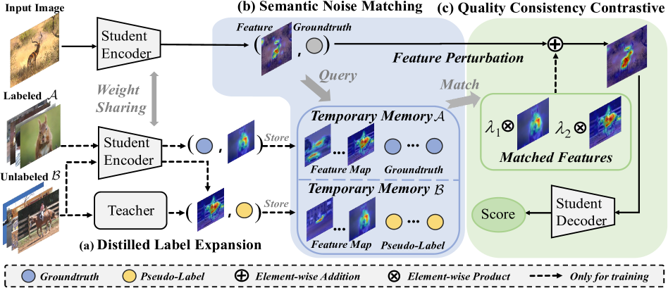
Figure 2: The overview of our QFM-IQM.We begin by extracting image quality-related features from the student network. Simultaneously, we indirectly augment our training set by introducing a distillation framework and storing the image features and labels in pairs in temporary memory (Sec. 3.4). We use Semantic Noisy Matching to select features in the temporary memory with similar quality but different quality scores as noise disturbance (Sec. 3.5) and add them to our original features as decoder input to predict image quality, forcing our model to learn to focus on quality-aware features (Sec. 3.6). During inference, scores are directly predicted using the encoder and decoder, while the Feature Diffusion Module with the distillation component is omitted.

2 Related Works

Image Quality Assessment (IQA) is broadly classified into full-reference (FR), reduced-reference (RR), and no-reference (NR) methods, as seen in works like [22, 28, 32, 43, 11]. While FR and RR methods, discussed in [2, 19, 38], rely on some level of reference to the original image, NR-IQA methods, such as those in [50, 48, 47, 24, 4, 40], operate independently, assessing image quality without a reference image. This makes NR-IQA more challenging but also more promising for real-world applications.

2.1 NR-IQA with Vision Transformer

Vision Transformer (ViT)  [7] has shown promising results on several downstream vision tasks. There are mainly two types of architectures for the ViT-based NR-IQA methods, including hybrid Transformer  [10] and pure ViT-based Transformer  [17]. The hybrid architecture generally combines the CNNs with the Transformer, which is responsible for the local and long-range feature characterization, respectively. For instance,  [10] proposed a hybrid Transformer for NR-IQA, where the multi-scale features extracted from ResNet-50 are fed to the transformer encoder to produce a non-local representation of the image. [17] designed a multi-scale ViT-based IQA model to handle the arbitrary size of input images. Such a feature encoder is initially designed to describe the image content, and thus the preserved features are mainly related to the higher-level visual abstractions which are not adequate in characterizing the quality-aware features of an image [31].

2.2 NR-IQA with Contrastive Learning

The goal of contrastive learning is to learn such an embedding space, where similar samples are attracted while dissimilar pairs are repelled [15, 49]. Notably, traditional contrastive learning can be classified as semantic-aware pre-training [3, 13], because it encourages views (augmentations) of the same image to have a similar representation while ignoring the changes in perceived image quality. Recently, contrastive learning in Image Quality Assessment (IQA) has primarily focused on unsupervised approaches, as seen in key studies like QPT [49], which introduces a self-supervised method with a quality-aware contrastive loss for BIQA. Re-IQA [33] employed a Mixture of Experts to train separate encoders for content and quality features, and CONTRIQUE [26] which used a deep CNN with a contrastive pairwise objective for robust NR-IQA. These methods have achieved promising results by leveraging self-supervised training, but the cost of pre-training models is often high. Different from the goal of these pre-trained models to learn general knowledge, our QFM-IQM focuses on the problem that distinguishing between images that have similar semantic features but different quality scores. This enhances the model’s recognition ability and robustness to noise from irrelevant features, thereby paving a new direction for supervised contrastive learning in NR-IQA.

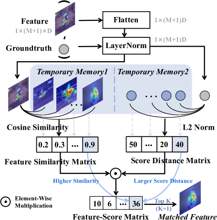
Figure 3: The Semantic Noise Feature Matching pipeline takes in pairs of features and labels as input and returns matching features from the dataset as output. Firstly, we flatten the input features and then normalize both the features and labels using layer norm. We then calculate the Feature Similarity Matrix and the Score Distance Matrix using the cosine similarity function and the $\mathcal{L}_{2}$ norm. Next, we obtain the final Feature-Score Matrix by element-wise multiplication of the computed matrices. We select the features that correspond to the index of the top K values of the largest Feature-Score Matrix in our memory as matched features.

3 Methodology

3.1 Preliminaries

In the context of No-Reference Image Quality Assessment (NR-IQA), we define some common notations. We use bold formatting to denote vectors (e.g., $\boldsymbol{x}$, $\boldsymbol{y}$) and matrices (e.g., $\boldsymbol{X}$, $\boldsymbol{Y}$). Specifically, $\boldsymbol{F}$ denotes the feature map of the network output, $\mathcal{F}$ denotes the vision transformer’s class token (cls token) [7], and Y denotes the quality score.

3.2 Overview

In this paper, we present Quality-Aware Feature Matching-based Image Quality Metric (QFM-IQM), a novel framework that can effectively distinguish between images with similar semantic features but different quality scores. As depicted in Fig. 2, QFM-IQM seamlessly integrates three main components: Semantic Noise Matching (SNM), Quality Consistency Contrastive (QCC) and Distillation Label Extension (DLE). Initially, the input distorted image is fed into a transformer encoder to obtain feature $\boldsymbol{F}_{o}\in\mathbb{R}^{(M+1)\times D}$ from the final layer. Subsequently, the SNM module matches these features with those that have similar semantics but different quality scores (Sec. 3.5). Next, the matched semantic noise is introduced as feature perturbation into feature $\boldsymbol{F}_{o}$ to obtain $\hat{\boldsymbol{F}_{o}}$ and the QCC module constraints between the quality prediction of the $\boldsymbol{F}_{o}$ and $\hat{\boldsymbol{F}_{o}}$ to remain consistent, forcing the model to be robust to quality-unrelated semantic noise during contrastive learning (Sec. 3.6). Additionally, the DLE module uses knowledge distillation to generate pseudo-labels for unlabeled samples, thereby enriching the contrastive learning dataset of QCC (Sec. 3.4). These components collectively contribute to a more effective and accurate NR-IQA process. It’s worth noting that during the inference process, scores are predicted directly using the encoder and decoder, discarding the above three modules, and avoiding any additional computational overhead.

3.3 Architecture Design

Transformer Encoder. Our model uses a Transformer encoder to process input image patches. These patches are first transformed into D-dimensional embeddings, including a class token and position embeddings for spatial information. Three linear projection layers transform patch embedding into matrices ${\boldsymbol{Q},\boldsymbol{K},\boldsymbol{V}}\in\mathbb{R}^{(M+1)\times D}$ for query, key, and value. This operation, combined with Multi-Head Self-Attention (MHSA), layer normalization, and a Multi-Layer Perceptron (MLP), produces the output feature $\boldsymbol{F}_{o}$.

Transformer Decoder. Previous works [31] found that CLS tokens cannot build an optimal representation for image quality. we utilize a quality-aware decoder that further interprets the CLS token. The decoder uses Multi-Head Cross-Attention (MHCA) with a set of queries $Q_{d}$, interacting with encoder outputs to calculate the final quality score $\boldsymbol{\hat{Y}}$. This method improves the learning and generalization capabilities of our NR-IQA model.

3.4 Distillation Label Extension

Considering the challenges transformer-based models face in learning sufficient downstream task knowledge with insufficient training data, leading to overfitting and performance degradation, this paper proposes a new distillation strategy. This strategy employs an extra unlabeled dataset $\mathcal{B}$ for feature contrastive learning during training, effectively using information from samples in the expanded dataset with similar features but different quality scores. Specifically, we first use a teacher model generating pseudo labels for each image in $\mathcal{B}$ and then store in a temporary memory $\mathcal{M}$. Then, datasets $\mathcal{A}$ and $\mathcal{B}$ are input into the student model together, identifying features with similar but different quality scores (refer to Sec. 3.5). These features, treated as noise, are added to the image features, enabling the model to learn from both labeled and unlabeled data and improve its generalization ability for new images with different quality scores.

3.5 Semantic Noise Feature Matching

In this section, we introduce our Semantic Noise Matching (SNM) Module and discuss how to match semantic noise samples that have feature aliasing.

Temporary Memory. The objective of the Temporary Memory $\mathcal{M}$ is to store features and labels of each mini-batch of data, serving as a queryable resource for the SNM module. Specifically, the student feature extractor conducts forward propagation to extract features of distorted images from dataset $\mathcal{A}$, and stores these features alongside the ground truth of the distorted images in Temporary Memory $\mathcal{A}$. Concurrently, the student extracts features of distorted images from dataset $\mathcal{B}$, storing them with the pseudo labels of these images in Temporary Memory $\mathcal{B}$. It is important to note that during the training process, the original memory data is overwritten in each iteration of every mini-batch to reset the Temporary Memory.

Semantic Noise Matching. Fig. 3 depicts the overview of our SNM module. As above mentioned, for a mini-batch input distorted image, the Temporary Memory $\mathcal{M}$ stores a collection of features and labels. Specifically, our QFM-IQM utilizes Semantic Noise Matching to select noise samples that have similar features but different quality scores from both the labeled datasets and unlabeled datasets, respectively, as illustrated in Fig. 3. This method, by explicitly considering the misalignment between features and quality scores, can select noise features that are irrelevant to quality perception. The process first flattens the feature ${\boldsymbol{F}}_{o}$ of the input image obtained by the encoder to obtain the feature vector ${\boldsymbol{f}}_{o}$, then another feature vector $\hat{{\boldsymbol{f}}}_{o}$ is obtained from the Temporary Memory $\mathcal{M}$. Next, the feature similarity is calculated using cosine distance, and the score distance is calculated using $\mathcal{L}_{2}$ norm; the resulting score $\mathcal{S}$ is obtained by multiplication of the feature similarity and score distance. The evaluation metric for the selection strategy can be expressed as:

$$\mathcal{S}((\boldsymbol{{f}}_{o},\rm{{y}}_{o}),(\boldsymbol{\hat{{f}}_{o}},\rm{\hat{{y}}_{o}}))=\frac{\boldsymbol{{f}}_{o}\cdot\hat{\boldsymbol{f}}_{o}}{\|\boldsymbol{{f}}_{o}\|\cdot\|\boldsymbol{\hat{{f}}_{o}}\|}\cdot\|\rm{{y}}_{o}-\rm{\hat{{y}}_{o}}\|.$$ (1)

Here, $\cdot$ represents the dot product between the vectors, and $\|\cdot\|$ represents their L2 norms. This score is then used as a criterion for the final selection strategy, choosing the top K maximum score features selected as matching samples for the Quality Consistency Contrastive module’s input.

3.6 Quality Consistency Contrastive

Existing studies have not addressed the challenge of differentiating between images with similar semantic features but different quality scores and eliminating quality-irrelevant features from high-level pre-trained features. To address this, we introduce the Quality Consistency Contrastive (QCC) module to isolate quality-related attributes from an image’s semantic content. In contrast to previous approaches that optimize contrastive learning loss based on InfoNCE, this paper introduces a straightforward yet effective method to enhance a model’s robustness to features unrelated to image quality. This is accomplished by strengthening the consistency of the model’s predictions for image quality before and after introducing noise to distorted images. This method reduces the model’s sensitivity to semantic noise and compels it to exhibit robustness to subtle variations, ultimately increasing the separation between feature representations of noise samples. Concretely, we initially extract the cls tokens of the top K features matched in the SNM module and incorporate them as feature perturbations into the original cls token. Since we perform feature selection twice in labeled dataset $\mathcal{A}$ and unlabelled dataset $\mathcal{B}$, the expression of this process is:

$${\mathcal{F}}=(1-{\lambda_{1}}-{\lambda_{2}}){{{\mathcal{F}}}_{o}}+\frac{\lambda_{1}}{K}\sum_{j=1}^{K}{\mathcal{\hat{F}}^{\mathcal{A}}_{o,j}}+\frac{\lambda_{2}}{K}\sum_{j=1}^{K}{\mathcal{\hat{F}}^{\mathcal{B}}_{o,j}},$$ (2)

where the weight $\lambda_{1}$ and $\lambda_{2}$ controls the strength of the perturbation. ${\mathcal{\hat{F}}^{\mathcal{A}}_{o,j}}$ and ${\mathcal{\hat{F}}^{\mathcal{B}}_{o,j}}$ represent the $j_{th}$ largest matching feature’s cls token from the labeled datasets $\mathcal{A}$ and unlabeled datasets $\mathcal{B}$, respectively. After that, we feed the feature ${\mathcal{F}}$ which is obtained by the above Eq. 2 into the transformer decoder to predict the quality score. It is noteworthy that the quality score predicted after noise addition is still supervised by the ground truth corresponding to the input image, which forces the model to be robust against the added semantic noise.

	LIVE		CSIQ		TID2013		KADID		LIVEC		KonIQ		LIVEFB		SPAQ
Method	PLCC	SRCC	PLCC	SRCC	PLCC	SRCC	PLCC	SRCC	PLCC	SRCC	PLCC	SRCC	PLCC	SRCC	PLCC	SRCC
DIIVINE  [32]	0.908	0.892	0.776	0.804	0.567	0.643	0.435	0.413	0.591	0.588	0.558	0.546	0.187	0.092	0.600	0.599
BRISQUE  [27]	0.944	0.929	0.748	0.812	0.571	0.626	0.567	0.528	0.629	0.629	0.685	0.681	0.341	0.303	0.817	0.809
ILNIQE  [44]	0.906	0.902	0.865	0.822	0.648	0.521	0.558	0.534	0.508	0.508	0.537	0.523	0.332	0.294	0.712	0.713
BIECON  [18]	0.961	0.958	0.823	0.815	0.762	0.717	0.648	0.623	0.613	0.613	0.654	0.651	0.428	0.407	-	-
MEON  [25]	0.955	0.951	0.864	0.852	0.824	0.808	0.691	0.604	0.710	0.697	0.628	0.611	0.394	0.365	-	-
WaDIQaM  [1]	0.955	0.960	0.844	0.852	0.855	0.835	0.752	0.739	0.671	0.682	0.807	0.804	0.467	0.455	-	-
DBCNN  [46]	0.971	0.968	0.959	0.946	0.865	0.816	0.856	0.851	0.869	0.851	0.884	0.875	0.551	0.545	0.915	0.911
TIQA  [42]	0.965	0.949	0.838	0.825	0.858	0.846	0.855	0.85	0.861	0.845	0.903	0.892	0.581	0.541	-	-
MetaIQA  [51]	0.959	0.960	0.908	0.899	0.868	0.856	0.775	0.762	0.802	0.835	0.887	0.850	0.507	0.54	-	-
P2P-BM  [41]	0.958	0.959	0.902	0.899	0.856	0.862	0.849	0.84	0.842	0.844	0.885	0.872	0.598	0.526	-	-
HyperIQA  [36]	0.966	0.962	0.942	0.923	0.858	0.840	0.845	0.852	0.882	0.859	0.917	0.906	0.602	0.544	0.915	0.911
TReS  [10]	0.968	0.969	0.942	0.922	0.883	0.863	0.858	0.859	0.877	0.846	0.928	0.915	0.625	0.554	-	-
MUSIQ  [16]	0.911	0.940	0.893	0.871	0.815	0.773	0.872	0.875	0.746	0.702	0.928	0.916	0.661	0.566	0.921	0.918
DACNN  [29]	0.980	0.978	0.957	0.943	0.889	0.871	0.905	0.905	0.884	0.866	0.912	0.901	-	-	0.921	0.915
DEIQT  [31]	0.982	0.980	0.963	0.946	0.908	0.892	0.887	0.889	0.894	0.875	0.934	0.921	0.663	0.571	0.923	0.919
QFM-IQM(ours)	0.983	0.981	0.965	0.954	0.932	0.916	0.906	0.906	0.913	0.891	0.936	0.922	0.667	0.567	0.924	0.920

Table 1: Performance comparison measured by averages of SRCC and PLCC, where bold entries indicate the best results, underlines indicate the second-best.

Training	LIVEFB		LIVEC	KonIQ	LIVE	CSIQ
Testing	KonIQ	LIVEC	KonIQ	LIVEC	CSIQ	LIVE
DBCNN	0.716	0.724	0.754	0.755	0.758	0.877
P2P-BM	0.755	0.738	0.74	0.77	0.712	-
HyperIQA	0.758	0.735	0.772	0.785	0.744	0.926
TReS	0.713	0.74	0.733	0.786	0.761	-
DEIQT	0.733	0.781	0.744	0.794	0.781	0.932
QFM-IQM	0.768	0.791	0.775	0.796	0.820	0.941

Table 2: SRCC on the cross datasets validation. The best performances are highlighted in boldface.

4 Experiments

4.1 Benchmark Datasets and Evaluation Protocols

We evaluate the QFM-IQM on eight standard NR-IQA datasets. These include four synthetic datasets: LIVE [35], CSIQ [20], TID2013 [30], and KADID [21]; and four authentic datasets: LIVEC [9], KONIQ [14], LIVEFB [41], and SPAQ [8]. The authentic datasets contain images captured by different photographers using various mobile devices, with LIVEC comprising 1162 images, SPAQ 11,125 images, and KONIQ-10k 10,073 images sourced from public multimedia resources. LIVEFB is the largest real-world dataset with 39,810 images. Synthetic datasets are generated by applying distortions like JPEG compression and Gaussian blur to original images. LIVE and CSIQ contain 779 and 866 images with five and six distortion types, respectively, while TID2013 and KADID have 3000 and 10,125 images with 24 and 25 distortion types. The performance of the QFM-IQM model, in terms of prediction accuracy and prediction monotonicity, is assessed using Spearman’s Order Correlation Coefficient (SRCC) and Pearson’s Linear Correlation Coefficient (PLCC). Both SRCC and PLCC values range from -1 to 1, with values near 1 denoting higher performance in both metrics.

4.2 Implementation Details

Pre-trained Teacher. Our teacher network, comprising a VIT-S and a decoder, is pre-trained on the KonIQ dataset for offline knowledge distillation on students trained on the LIVEFB dataset. For training on the other seven datasets, the NR teacher pre-trained on LIVEFB is used.

Student Training. To train the student network, we follow the standard approach of cropping input images into ten 224x224 patches, reshaped into smaller 16x16 patches with a 384-dimensional input token. Using a Transformer encoder based on ViT-S from DeiT III [39], our model has 12 layers and 6 heads, coupled with a single-layer decoder. Training is conducted over 9 epochs with a learning rate of $2\times 10^{-4}$, reducing by a factor of 10 every 3 epochs, using the Adamw optimizer [23]. Batch size ranges from 16 128, with an 80/20 split for training and testing. This process is repeated ten times to minimize bias. For synthetic distortion datasets, training and testing sets are divided by reference images for content independence. The model’s performance is quantified by the average SRCC and PLCC, measuring prediction accuracy and monotonicity.

4.3 Overall Prediction Performance Comparison

The results of the comparison between QFM-IQM and 15 classical or state-of-the-art NR-IQA methods, which include hand-crafted feature-based NR-IQA methods like ILNIQE  [44] and BRISQUE  [27], as well as deep learning-based methods such as MUSIQ  [16] and DEIQT  [31], are presented in Table 1. It can be observed across the 8 datasets that QFM-IQM outperforms all other methods in terms of performance. Achieving competitive performance on all of these datasets is a challenging task due to the wide range of image content and distortion types. Therefore, these observations confirm the effectiveness and superiority of QFM-IQM in accurately characterizing image quality.

4.4 Generalization Capability Validation

To assess the generalization capabilities of QFM-IQM, we carried out a series of cross-dataset validation experiments. In these tests, QFM-IQM was trained on one dataset and then evaluated on different datasets without any adjustments to its parameters. The comprehensive results, presented in Table 2, demonstrate QFM-IQM’s superior performance over state-of-the-art models across six datasets. This includes notable gains on the LIVEC dataset and strong results on the KonIQ dataset. These results, enhanced by the extensive contrastive knowledge about various distortions provided by the DLE module, underscore QFM-IQM’s exceptional ability to generalize.

Index	$\mathcal{A}^{QCC}$	$\mathcal{B}^{QCC}$	TID2013		LIVEC		KonIQ
			PLCC	SRCC	PLCC	SRCC	PLCC	SRCC
a)			0.899 (±0.017)	0.891 (±0.028)	0.883 (±0.012)	0.865 (±0.021)	0.926 (±0.003)	0.913 (±0.003)
b)	✔		0.919 (±0.022)	0.901 (±0.026)	0.904 (±0.009)	0.885 (±0.011)	0.934 (±0.001)	0.922 (±0.002)
c)		✔	0.925 (±0.016)	0.910 (±0.022)	0.907 (±0.006)	0.882 (±0.010)	0.935 (±0.002)	0.921 (±0.002)
d)	✔	✔	0.932 (±0.015)	0.916 (±0.017)	0.913 (±0.007)	0.891 (±0.009)	0.936 (±0.002)	0.922 (±0.003)

Table 3: Ablation experiments on TID2013, LIVEC and KonIQ datasets. Here, $\mathcal{A}^{QCC}$ and $\mathcal{B}^{QCC}$ refer to the Quality Consistency Contrastive without and with the Distillation Label Extension module, where bold entries indicate the best result.

4.5 Ablation Study

The core idea of our QFM-IQM is to improve the model’s ability to distinguish subtle quality differences by enhancing its robustness to semantic noise. Therefore, we explored the impact of Quality Consistency Contrastive (QCC) operation on the model when compared with different datasets in Table 3. Let $\mathcal{A}^{QCC}$ denote the QCC operation only compare with the labeled dataset $\mathcal{A}$, and $\mathcal{B}^{QCC}$ denote the QCC operation only compare with the unlabeled dataset $\mathcal{B}$.

Effective on labeled dataset $\mathcal{A}$ We explored the effectiveness of the QCC module on the original training dataset. After contrastive learning, performance on three datasets improved to varying degrees. Particularly on the LIVEC real dataset, there was a significant improvement of 2.1 points, and the variance was significantly reduced. However, we found that on the TID2013 synthetic dataset, although there was a significant improvement of 2 points, the stability of the model decreased. We analyze this as due to the synthetic dataset having less rich semantic information than the real dataset, causing our QCC module to force the model to ignore the quality-related semantic information, thereby weakening its stability.

Effective on unlabeled dataset $\mathcal{B}$ We further investigated the effectiveness of the QCC module on the expanded unlabeled training dataset. Compared to $\mathcal{A}^{QCC}$, $\mathcal{B}^{QCC}$ achieved more significant performance improvements. Additionally, the issue of decreased stability on the TID2013 dataset was rectified, ensuring stability across all datasets. This indicates that using additional pseudo-labels to expand our dataset allows our QFM-IQM to learn from images with different quality levels and feature distributions. Consequently, our model can distinguish quality-related features through more extensive data comparisons. The combination of $\mathcal{A}^{QCC}$ and $\mathcal{B}^{QCC}$ leads to a state-of-the-art deep learning model for image quality assessment.

Figure 4: Qualitative analysis on image pairs have similar semantic features but different quality scores. The bar charts in (a) and (b) display the number of image pairs with the most similar features within a specific label distance range. For TReS, there are many image pairs with similar features but large differences in quality scores (even with label distance greater than 30, TReS considers 52 samples as feature-similar). Our model greatly alleviates this issue and achieves a lead in accuracy (a large number of light yellow areas represent smaller prediction errors). In bar char (c), we integrated the statistical results of (a) and (b) to make the above conclusions clearer.

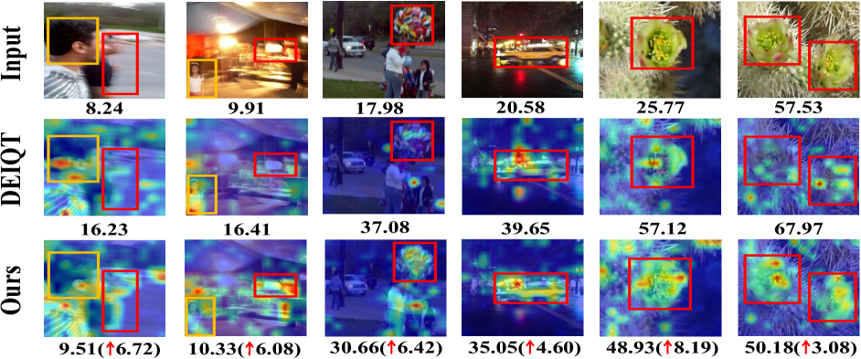
Figure 5: Activation maps of DEIQT  [31] and QFM-IQM using Grad-CAM  [34] on authentic dataset LIVEC. The scores in the figure represent Mean Opinion Scores (MOS). Our model pays more attention to image distortion regions (red boxes) and is less sensitive to semantic noise (yellow boxes), and correspondingly our image quality prediction ability is closer to the true value. Rows 1-3 represent input images, CAMs from DEIQT  [31], and CAMs from QFM-IQM, respectively.

4.6 Qualitative Analysis

Analyze similar features that have different quality.  In Fig. 4, sections (a) and (b) display the number of image pairs with the most similar features within a specific label distance range in the dataset, as determined by the TReS and QFM-IQM models. The vertical axis in these graphs represents the number, while the horizontal axis shows the range of label differences. Specifically, in Fig.4(a), it’s noted that out of 1162 distorted images in the LIVEC dataset, 52 images exhibit similar features that have a considerable quality score difference of over 30. This finding highlights a common issue where similar features do not necessarily correspond to similar quality scores. This discrepancy could be due to the presence of only a few quality-relevant features influencing the model’s evaluation. Moreover, Fig.4(c) conducts a summary statistic of (a) and (b), and demonstrates the effectiveness of our proposed model in addressing this issue. The QFM-IQM model achieves a notable reduction, approximately 56%, in the number of similar features with significant score differences when compared to the TReS model. Additionally, there’s an increase of about 16.3% in the number of similar features having closer scores. This improvement leads to a better positive correlation and, consequently, enhances the overall quality prediction performance of the model. In summary, our model gives more weight to quality-related features than the TReS model. This approach results in a higher inclusion of quality-related features in the extracted feature set and significantly reduces the bias in quality estimation.

Visualization of class activation map. We utilized GradCAM [34] to visualize the feature attention maps in Figure 5. The results show that our model accurately and comprehensively focuses on the distorted regions (including both quality-related semantic degradations and low-level artifacts), while DEIQT [31] fails to accurately pinpoint the true areas of quality degradation. This indicates that our model excels in learning the subtle differences between semantic structures and quality-aware features. We achieved this by filtering out features irrelevant to quality from the pre-trained model, focusing on learning those quality-aware features that are pertinent to quality prediction.

4.7 Analysis of the K in Memory Searching

In this analysis, we examine the effect of the memory searching operation’s searching number, K. We conduct experiments on both synthetic and real distortion datasets, LIVE and LIVEC, with K values of 1, 2, 3, 4, 6, and 8. The results, as shown in Table 4, demonstrate that the performance on holistic IQA datasets remains stable with various K values, with only a slight fluctuation within 1%.

	LIVE		LIVEC
K-NN	PLCC	SRCC	PLCC	SRCC
K=1	0.983	0.981	0.910	0.887
K=2	0.981	0.978	0.905	0.887
K=3	0.982	0.979	0.900	0.880
K=4	0.982	0.980	0.904	0.885
K=6	0.981	0.978	0.913	0.891
K=8	0.978	0.976	0.903	0.877

Table 4: Analysis of the K in memory searching on both real and synthetic datasets. Bold entries indicate the best performance.

Specifically, in the synthetic dataset LIVE, which comprises only 30 distinct content images, the types of distortions (like Gaussian blur and JPEG) are generally uniform across the whole image, so the model receives relatively less contamination at the semantic level, hence setting K to 1 can achieve the best results. On the other hand, in the authentic dataset LIVEC, since all the training data contain different contents which leads to various semantic level degradations. Therefore, how to effectively utilize quality perception features from pre-trained semantic features is particularly important, so we find that the best performance can be achieved by setting the K value to 6. However, setting the K value too high can also have a negative impact. When too much noise is added, the original features of the image learned by the model can be affected.

4.8 Sensitivity study of hyper-parameters

	LIVE		LIVEC		konIQ
Weight	PLCC	SRCC	PLCC	SRCC	PLCC	SRCC
E-1	0.978	0.976	0.884	0.857	0.925	0.911
E-2	0.979	0.976	0.877	0.865	0.934	0.919
E-4	0.979	0.979	0.897	0.875	0.931	0.916
E-5	0.980	0.978	0.904	0.884	0.932	0.917
E-7	0.983	0.981	0.910	0.887	0.936	0.922
E-8	0.981	0.979	0.902	0.886	0.933	0.917

Table 5: Sensitivity study of hyper-parameters on LIVE, LIVEC, and KonIQ datasets. Bold entries indicate the best performance.

In this paper, we use ${\lambda_{1}}$ and ${\lambda_{2}}$ in Eq. 2 to balance the contrastive Learning and distillation, respectively. In this subsection, we do the sensitivity study on different feature perturbation weights ${\lambda_{1}}$ to explore the effect of QCC, maintaining the search number K at 1. As presented in Table 5, our findings reveal that the QCC module has relatively low sensitivity to the hyperparameters. Specifically, small values of $\lambda$ weaken our QCC’s impact, whereas large values of $\lambda$ cause significant changes in the feature space and result in performance degradation on the LIVEC dataset.

5 Conclusion

In this paper, we propose a novel method named QFM-IQM for no-reference image quality assessment, which addresses the common challenge of distinguishing between images with similar semantic features but different quality scores and isolates the quality-related attributes from the semantic content of an image. This is achieved through the design of a quality consistency contrastive module that selects images with similar features but large quality score gaps as feature perturbations, which force the student model to capture the subtle differences in quality among similar images. In addition, QFM-IQM employs distillation learning to augment the dataset with authentic images, improving the model’s generalization ability across different domains and scenarios. Our experiments on eight benchmark IQA datasets demonstrate the superiority of the proposed approach.

Appendix A Appendix Overview

The supplementary material is organized as follows: Qualitative Analysis provides more analysis of the effectiveness of the QFM-IQM and is further illustrated in conjunction with our motivation. Training and Evaluation Details: shows more training and evaluation details. Comparison with CONTRIQUE: provides more analysis of existing methods CONTRIQUE [26] based on contrastive learning.

Appendix B Qualitative Analysis

In this section, we provide an additional explanation about the content of Fig. 6 to help readers understand our motivation. Our motivation stems from a phenomenon we discovered through experimentation: existing state-of-the-art (SOTA) models based on pre-training, such as TReS, struggle to adequately distinguish the feature distances between image pairs with different quality scores. This results in inaccurate quality predictions. As shown in Fig. 6(a), TReS mistakenly identifies image pairs with a quality score difference greater than 30 as having very similar features. We believe this may be due to feature confusion, where current models are misled by the similar semantics of the image pairs, leading them to perceive similar features in images with different quality scores, thereby failing to adequately separate their features. This results in erroneous quality predictions. Our method addresses this feature confusion by specifically designing for it. We select noisy samples with different quality scores but similar semantic features, and through noise perturbation, force the model to reduce its sensitivity to them. This effectively increases the feature distance between image pairs with similar semantics but different quality scores. As illustrated in Fig. 6(b), our QFM-IQM significantly mitigates the aforementioned issue. Specifically, it alleviates the situation where image pairs with a quality score difference greater than 30 still share very similar features, and the correlation between features and quality scores is more positively aligned, meaning similar quality scores have similar quality features. Additionally, the error in our quality predictions is smaller, further demonstrating the effectiveness of our approach.

Dataset	Resolution	Resize	Batch Size	Label Range
LIVE [35]	$768\times 512$	$512\times 384$	12	DMOS [0,100]
CSIQ [20]	$512\times 512$	$512\times 512$	12	DMOS [0,1]
TID2013 [30]	$512\times 384$	$512\times 384$	48	MOS [0,9]
KADID [21]	$512\times 384$	$512\times 384$	128	MOS [1,5]
LIVEC [9]	$500P\sim 640P$	$500P\sim 640P$	16	MOS [1,100]
KonIQ [14]	$768P$	$512\times 384$	128	MOS [0,5]
LIVEFB [41]	$160P\sim 700P$	$512\times 512$	128	MOS [0,100]
SPAQ  [8]	$1080P\sim 4368P$	$512\times 384$	128	MOS [0,100]

Table 6: Training preprocessing details of selected BIQA datasets.

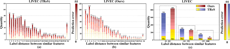
Figure 6: Qualitative analysis on image pairs have similar semantic features but different quality scores. The bar charts in (a) and (b) display the number of image pairs with the most similar features within a specific label distance range. For TReS, there are many image pairs with similar features but large differences in quality scores (even with label distance greater than 30, TReS considers 52 samples as feature-similar). Our model greatly alleviates this issue and achieves a lead in accuracy (a large number of light yellow areas represent smaller prediction errors). In bar char (c), we integrated the statistical results of (a) and (b) to make the above conclusions clearer.

	LIVE		CSIQ		TID2013		KADID		LIVEC		KonIQ		LIVEFB		SPAQ
Method	PLCC	SRCC	PLCC	SRCC	PLCC	SRCC	PLCC	SRCC	PLCC	SRCC	PLCC	SRCC	PLCC	SRCC	PLCC	SRCC
CONTRIQUE	0.961	0.960	0.955	0.942	0.857	0.843	0.937	0.934	0.857	0.845	0.906	0.894	0.641	0.580	0.919	0.914
QFM-IQM(ours)	0.983	0.981	0.965	0.954	0.932	0.916	0.906	0.906	0.913	0.891	0.936	0.922	0.667	0.567	0.924	0.920

Table 7: Performance comparison measured by averages of SRCC and PLCC, where bold entries indicate the best results.

	KonIQ		LIVEFB
Method	PLCC	SRCC	PLCC	SRCC
QFM-IQM	0.936	0.922	0.667	0.567
Teacher	0.930	0.914	0.667	0.566

Table 8: Performance comparison measured by averages of SRCC and PLCC, where bold entries indicate the best results.

Appendix C Training and Evaluation Details

Efficacy of subcomponents in the training phase: Our Distilled Label Expansion augments the dataset using authentic images of different quality levels on LIVEFB and KonIQ to overcome the lack of sufficient training data in IQA. Our Semantic Noise Feature Matching compares the features of input with other features to match similar semantics but different quality features (Fig.3 of the main paper). These matched features are considered noises to be added to the original features in the process of Quality Consistency Contrastive. Our Quality Consistency Contrastive constrains the model to still be supervised by the ground truth for the quality prediction of the noise-added samples. This enables the model to emphasize the subtle differences among distortion images, while concurrently reducing the significance placed on semantic aspects.

Unlabeled data: Our unlabeled data comes from the LIVEFB and KonIQ datasets, but we do not use the label information provided by these datasets during training. During training, we randomly sample a mini-batch of unlabeled images for training.

Implement details of training phrase: To train the student network, we adopt a standard approach of randomly cropping input images into ten patches, each with a $224\times 224$ resolution. Subsequently, we reshape these patches into a sequence of smaller patches with a patch size of p = 16 and an input token dimension of D = 384. Furthermore, we present additional training preprocessing details for various datasets, which are not included in the main paper, in Tab. 6. For different benchmarks, we employ different training settings for a fair comparison.

Teacher performance: We ensured the high accuracy of the pre-trained teacher model on the dataset to provide reliable pseudo-labels, as shown in Table 8.

Inference phrase: During the inference process, we only employ a trained encoder-decoder architecture to directly assess the image’s quality which benefits from the QFM-IQM to precisely isolate quality-aware features within the pre-trained semantic feature space, thereby enhancing the accuracy of our quality predictions.

Training	Testing	CONTRIQUE	QFM-IQM
LIVEC	KonIQ	0.676	0.775
KonIQ	LIVEC	0.731	0.796
LIVE	CSIQ	0.823	0.820
CSIQ	LIVE	0.925	0.941

Table 9: SRCC on the cross datasets validation. The best results are highlighted in bold.

Appendix D Comparison with CONTRIQUE

Our approach differs significantly from CONTRIQUE. In CONTRIQUE, the approach revolves around treating the IQA representation learning problem as a classification task. In this framework, images are categorized into various classes based on distortion types, and contrastive loss is utilized to learn distinctive features that can discriminate between these classes. However, a limitation of this approach is that each real image is treated as a separate class, which doesn’t allow for the effective mining of information from distorted images with similar quality. In contrast, our method does not fixate on specific distortion types. Instead, it takes into account differences in quality scores, avoiding the aforementioned limitation. We achieve this by comparing images and selecting those with similar semantic features but varying quality scores. These selected images are then fused with the original features as a form of noise, with the aim of diminishing their semantic importance. This approach effectively separates the attributes related to image quality from the semantic features. As shown in Tab.9 and Tab.7), our QFM-IQM shows better performance on performance comparison and cross-dataset validation experiments. Specifically, it surpasses $\uparrow 7.5\%$ vs. 0.857 on TID2013 and $\uparrow 5.3\%$ vs. 0.857 on LIVEC, which demonstrates the superiority of our method.

References

- Bosse et al. [2017] Sebastian Bosse, Dominique Maniry, Klaus-Robert Müller, Thomas Wiegand, and Wojciech Samek. Deep neural networks for no-reference and full-reference image quality assessment. IEEE Transactions on image processing, 27(1):206–219, 2017.
- Cao et al. [2022] Yue Cao, Zhaolin Wan, Dongwei Ren, Zifei Yan, and Wangmeng Zuo. Incorporating semi-supervised and positive-unlabeled learning for boosting full reference image quality assessment. In Proceedings of the IEEE/CVF Conference on Computer Vision and Pattern Recognition, pages 5851–5861, 2022.
- Caron et al. [2020] Mathilde Caron, Ishan Misra, Julien Mairal, Priya Goyal, Piotr Bojanowski, and Armand Joulin. Unsupervised learning of visual features by contrasting cluster assignments. Advances in neural information processing systems, 33:9912–9924, 2020.
- Chen et al. [2020] Diqi Chen, Yizhou Wang, and Wen Gao. No-reference image quality assessment: An attention driven approach. IEEE Transactions on Image Processing, 29:6496–6506, 2020.
- Deng et al. [2009] Jia Deng, Wei Dong, Richard Socher, Li-Jia Li, Kai Li, and Li Fei-Fei. Imagenet: A large-scale hierarchical image database. In 2009 IEEE conference on computer vision and pattern recognition, pages 248–255. Ieee, 2009.
- Ding et al. [2020] Keyan Ding, Kede Ma, Shiqi Wang, and Eero P Simoncelli. Image quality assessment: Unifying structure and texture similarity. IEEE transactions on pattern analysis and machine intelligence, 44(5):2567–2581, 2020.
- Dosovitskiy et al. [2021] Alexey Dosovitskiy, Lucas Beyer, Alexander Kolesnikov, Dirk Weissenborn, Xiaohua Zhai, Thomas Unterthiner, Mostafa Dehghani, Matthias Minderer, Georg Heigold, Sylvain Gelly, Jakob Uszkoreit, and Neil Houlsby. An image is worth 16x16 words: Transformers for image recognition at scale. In International Conference on Learning Representations, 2021.
- Fang et al. [2020] Yuming Fang, Hanwei Zhu, Yan Zeng, Kede Ma, and Zhou Wang. Perceptual quality assessment of smartphone photography. In Proceedings of the IEEE/CVF Conference on Computer Vision and Pattern Recognition, pages 3677–3686, 2020.
- Ghadiyaram and Bovik [2015] Deepti Ghadiyaram and Alan C Bovik. Massive online crowdsourced study of subjective and objective picture quality. IEEE Transactions on Image Processing, 25(1):372–387, 2015.
- Golestaneh et al. [2022] S Alireza Golestaneh, Saba Dadsetan, and Kris M Kitani. No-reference image quality assessment via transformers, relative ranking, and self-consistency. In Proceedings of the IEEE/CVF Winter Conference on Applications of Computer Vision, pages 1220–1230, 2022.
- Gu et al. [2014] Ke Gu, Guangtao Zhai, Xiaokang Yang, and Wenjun Zhang. Using free energy principle for blind image quality assessment. IEEE Transactions on Multimedia, 17(1):50–63, 2014.
- Gu et al. [2020] Shuyang Gu, Jianmin Bao, Dong Chen, and Fang Wen. Giqa: Generated image quality assessment. In Computer Vision–ECCV 2020: 16th European Conference, Glasgow, UK, August 23–28, 2020, Proceedings, Part XI 16, pages 369–385. Springer, 2020.
- He et al. [2020] Kaiming He, Haoqi Fan, Yuxin Wu, Saining Xie, and Ross Girshick. Momentum contrast for unsupervised visual representation learning. In Proceedings of the IEEE/CVF conference on computer vision and pattern recognition, pages 9729–9738, 2020.
- Hosu et al. [2020] Vlad Hosu, Hanhe Lin, Tamas Sziranyi, and Dietmar Saupe. Koniq-10k: An ecologically valid database for deep learning of blind image quality assessment. IEEE Transactions on Image Processing, 29:4041–4056, 2020.
- Jaiswal et al. [2020] Ashish Jaiswal, Ashwin Ramesh Babu, Mohammad Zaki Zadeh, Debapriya Banerjee, and Fillia Makedon. A survey on contrastive self-supervised learning. Technologies, 9(1):2, 2020.
- Ke et al. [2021a] Junjie Ke, Qifei Wang, Yilin Wang, Peyman Milanfar, and Feng Yang. Musiq: Multi-scale image quality transformer. In Proceedings of the IEEE/CVF International Conference on Computer Vision, pages 5148–5157, 2021a.
- Ke et al. [2021b] Junjie Ke, Qifei Wang, Yilin Wang, Peyman Milanfar, and Feng Yang. Musiq: Multi-scale image quality transformer. In Proceedings of the IEEE/CVF International Conference on Computer Vision, pages 5148–5157, 2021b.
- Kim and Lee [2016] Jongyoo Kim and Sanghoon Lee. Fully deep blind image quality predictor. IEEE Journal of selected topics in signal processing, 11(1):206–220, 2016.
- Kim et al. [2020] Woojae Kim, Anh-Duc Nguyen, Sanghoon Lee, and Alan Conrad Bovik. Dynamic receptive field generation for full-reference image quality assessment. IEEE Transactions on Image Processing, 29:4219–4231, 2020.
- Larson and Chandler [2010] Eric Cooper Larson and Damon Michael Chandler. Most apparent distortion: full-reference image quality assessment and the role of strategy. Journal of electronic imaging, 19(1):011006, 2010.
- Lin et al. [2019] Hanhe Lin, Vlad Hosu, and Dietmar Saupe. Kadid-10k: A large-scale artificially distorted iqa database. In 2019 Eleventh International Conference on Quality of Multimedia Experience (QoMEX), pages 1–3. IEEE, 2019.
- Liu et al. [2013] Xinhao Liu, Masayuki Tanaka, and Masatoshi Okutomi. Single-image noise level estimation for blind denoising. IEEE Trans. Image Process., 22(12):5226–5237, 2013.
- Loshchilov and Hutter [2019] Ilya Loshchilov and Frank Hutter. Decoupled weight decay regularization. In International Conference on Learning Representations, 2019.
- Ma et al. [2021] Jupo Ma, Jinjian Wu, Leida Li, Weisheng Dong, Xuemei Xie, Guangming Shi, and Weisi Lin. Blind image quality assessment with active inference. IEEE Transactions on Image Processing, 30:3650–3663, 2021.
- Ma et al. [2017] Kede Ma, Wentao Liu, Kai Zhang, Zhengfang Duanmu, Zhou Wang, and Wangmeng Zuo. End-to-end blind image quality assessment using deep neural networks. IEEE Transactions on Image Processing, 27(3):1202–1213, 2017.
- Madhusudana et al. [2022] Pavan C Madhusudana, Neil Birkbeck, Yilin Wang, Balu Adsumilli, and Alan C Bovik. Image quality assessment using contrastive learning. IEEE Transactions on Image Processing, 31:4149–4161, 2022.
- Mittal et al. [2012] Anish Mittal, Anush Krishna Moorthy, and Alan Conrad Bovik. No-reference image quality assessment in the spatial domain. IEEE Transactions on image processing, 21(12):4695–4708, 2012.
- Moorthy and Bovik [2011] Anush Krishna Moorthy and Alan Conrad Bovik. Blind image quality assessment: From natural scene statistics to perceptual quality. IEEE Trans. Image Process., 20(12):3350–3364, 2011.
- Pan et al. [2022] Zhaoqing Pan, Hao Zhang, Jianjun Lei, Yuming Fang, Xiao Shao, Nam Ling, and Sam Kwong. Dacnn: Blind image quality assessment via a distortion-aware convolutional neural network. IEEE Transactions on Circuits and Systems for Video Technology, 32(11):7518–7531, 2022.
- Ponomarenko et al. [2015] Nikolay Ponomarenko, Lina Jin, Oleg Ieremeiev, Vladimir Lukin, Karen Egiazarian, Jaakko Astola, Benoit Vozel, Kacem Chehdi, Marco Carli, Federica Battisti, et al. Image database tid2013: Peculiarities, results and perspectives. Signal processing: Image communication, 30:57–77, 2015.
- Qin et al. [2023] Guanyi Qin, Runze Hu, Yutao Liu, Xiawu Zheng, Haotian Liu, Xiu Li, and Yan Zhang. Data-efficient image quality assessment with attention-panel decoder. In Proceedings of the Thirty-Seventh AAAI Conference on Artificial Intelligence, 2023.
- Saad et al. [2012] Michele A Saad, Alan C Bovik, and Christophe Charrier. Blind image quality assessment: A natural scene statistics approach in the dct domain. IEEE transactions on Image Processing, 21(8):3339–3352, 2012.
- Saha et al. [2023] Avinab Saha, Sandeep Mishra, and Alan C Bovik. Re-iqa: Unsupervised learning for image quality assessment in the wild. In Proceedings of the IEEE/CVF Conference on Computer Vision and Pattern Recognition, pages 5846–5855, 2023.
- Selvaraju et al. [2017] Ramprasaath R Selvaraju, Michael Cogswell, Abhishek Das, Ramakrishna Vedantam, Devi Parikh, and Dhruv Batra. Grad-cam: Visual explanations from deep networks via gradient-based localization. In Proceedings of the IEEE international conference on computer vision, pages 618–626, 2017.
- Sheikh et al. [2006] Hamid R Sheikh, Muhammad F Sabir, and Alan C Bovik. A statistical evaluation of recent full reference image quality assessment algorithms. IEEE Transactions on image processing, 15(11):3440–3451, 2006.
- Su et al. [2020] Shaolin Su, Qingsen Yan, Yu Zhu, Cheng Zhang, Xin Ge, Jinqiu Sun, and Yanning Zhang. Blindly assess image quality in the wild guided by a self-adaptive hyper network. In Proceedings of the IEEE/CVF Conference on Computer Vision and Pattern Recognition, pages 3667–3676, 2020.
- Talebi and Milanfar [2018] Hossein Talebi and Peyman Milanfar. Nima: Neural image assessment. IEEE transactions on image processing, 27(8):3998–4011, 2018.
- Tao et al. [2009] Dacheng Tao, Xuelong Li, Wen Lu, and Xinbo Gao. Reduced-reference iqa in contourlet domain. IEEE Transactions on Systems, Man, and Cybernetics, Part B (Cybernetics), 39(6):1623–1627, 2009.
- Touvron et al. [2022] Hugo Touvron, Matthieu Cord, and Hervé Jégou. Deit iii: Revenge of the vit. arXiv preprint arXiv:2204.07118, 2022.
- Wu et al. [2020] Jinjian Wu, Jupo Ma, Fuhu Liang, Weisheng Dong, Guangming Shi, and Weisi Lin. End-to-end blind image quality prediction with cascaded deep neural network. IEEE Transactions on image processing, 29:7414–7426, 2020.
- Ying et al. [2020] Zhenqiang Ying, Haoran Niu, Praful Gupta, Dhruv Mahajan, Deepti Ghadiyaram, and Alan Bovik. From patches to pictures (paq-2-piq): Mapping the perceptual space of picture quality. In Proceedings of the IEEE/CVF Conference on Computer Vision and Pattern Recognition, pages 3575–3585, 2020.
- You and Korhonen [2021] Junyong You and Jari Korhonen. Transformer for image quality assessment. In 2021 IEEE International Conference on Image Processing (ICIP), pages 1389–1393. IEEE, 2021.
- Zhai et al. [2011] Guangtao Zhai, Xiaolin Wu, Xiaokang Yang, Weisi Lin, and Wenjun Zhang. A psychovisual quality metric in free-energy principle. IEEE Trans. Image Process., 21(1):41–52, 2011.
- Zhang et al. [2015a] Lin Zhang, Lei Zhang, and Alan C Bovik. A feature-enriched completely blind image quality evaluator. IEEE Transactions on Image Processing, 24(8):2579–2591, 2015a.
- Zhang et al. [2015b] Peng Zhang, Wengang Zhou, Lei Wu, and Houqiang Li. Som: Semantic obviousness metric for image quality assessment. In Proceedings of the IEEE Conference on Computer Vision and Pattern Recognition, pages 2394–2402, 2015b.
- Zhang et al. [2018] Weixia Zhang, Kede Ma, Jia Yan, Dexiang Deng, and Zhou Wang. Blind image quality assessment using a deep bilinear convolutional neural network. IEEE Transactions on Circuits and Systems for Video Technology, 30(1):36–47, 2018.
- Zhang et al. [2021] Weixia Zhang, Kede Ma, Guangtao Zhai, and Xiaokang Yang. Uncertainty-aware blind image quality assessment in the laboratory and wild. IEEE Transactions on Image Processing, 30:3474–3486, 2021.
- Zhang et al. [2022] Weixia Zhang, Dingquan Li, Chao Ma, Guangtao Zhai, Xiaokang Yang, and Kede Ma. Continual learning for blind image quality assessment. IEEE Transactions on Pattern Analysis and Machine Intelligence, 2022.
- Zhao et al. [2023] Kai Zhao, Kun Yuan, Ming Sun, Mading Li, and Xing Wen. Quality-aware pre-trained models for blind image quality assessment. In Proceedings of the IEEE/CVF Conference on Computer Vision and Pattern Recognition, pages 22302–22313, 2023.
- Zheng et al. [2021] Heliang Zheng, Huan Yang, Jianlong Fu, Zheng-Jun Zha, and Jiebo Luo. Learning conditional knowledge distillation for degraded-reference image quality assessment. In Proceedings of the IEEE/CVF International Conference on Computer Vision, pages 10242–10251, 2021.
- Zhu et al. [2020] Hancheng Zhu, Leida Li, Jinjian Wu, Weisheng Dong, and Guangming Shi. Metaiqa: Deep meta-learning for no-reference image quality assessment. In Proceedings of the IEEE/CVF Conference on Computer Vision and Pattern Recognition, pages 14143–14152, 2020.